Ultimate phase estimation in a squeezed-state interferometer using photon counters with a finite number resolution

Abstract

Photon counting measurement has been regarded as the optimal measurement scheme for phase estimation in the squeezed-state interferometry, since the classical Fisher information equals to the quantum Fisher information and scales as $\bar{n}^{2}$ for given input number of photons $\bar{n}$. However, it requires photon-number-resolving detectors with a large enough resolution threshold. Here we show that a collection of $N$-photon detection events for $N$ up to the resolution threshold $\sim\bar{n}$ can result in the ultimate estimation precision beyond the shot-noise limit. An analytical formula has been derived to obtain the best scaling of the Fisher information.

I Introduction

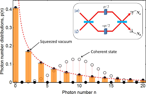
Quantum phase estimation through a two-path interferometer (e.g., the widely adopted Mach-Zehnder interferometer) is well-known inferred from the intensity difference between the two output ports. With a coherent-state light input, the Cramér-Rao lower bound of phase sensitivity can only reach the shot-noise (or classical) limit Helstrom ; Kay ; Braunstein ; Luo ; Smerzi09 ; Giovannetti , $\delta\varphi_{\mathrm{CRB}}=1/\sqrt{F(\varphi)}\sim 1/\sqrt{\bar{n}}$, where $F(\varphi)\sim O(\bar{n})$ denotes the classical Fisher information and $\bar{n}$ is the mean photon number. To beat the classical limit, Caves Caves proposed a squeezed-state interferometer by feeding a coherent state $|\alpha\rangle$ into one port and a squeezed vacuum $|\xi\rangle$ into the other port, as illustrated by the inset of Fig. 1, which is of particular interest for high-precision gravitational waves detection Caves ; Aasi and new generation of fountain clocks based on atomic squeezed vacuum Kruse ; Peise .

Theoretically, Pezzé and Smerzi Smerzi08 have shown that photon-counting measurement is optimal in the squeezed-state interferometer, since the classical Fisher information (CFI) equals to the quantum Fisher information (QFI) and scales as $\bar{n}^{2}$, leading to the ultimate precision in the Heisenberg limit $\delta\varphi_{\mathrm{CRB}}\sim 1/\bar{n}$. Recently, the phase-matching condition that maximizes the QFI has been investigated Liu . Lang and Caves Lang proved that under a constraint on $\bar{n}$, if a coherent-state light is fed from one input port, then the squeezed vacuum is the optimal state from the second port.

The theoretical bound in the phase estimation Smerzi08 ; Liu ; Lang has been derived by assuming photon-number-resolving detectors (PNRDs) with a exactly perfect number resolution Seshadreesan . However, the best detector up to date can only resolve the number of photons up to $4$ Smerzi07 ; Kardynal . Such a resolution threshold is large enough to realize coherent-state light interferometry with a low brightness input $\bar{n}\simeq 1$ Smerzi07 . To achieve a high-precision quantum metrology, nonclassical resource with large number of particles is one of the most needed Slusher1985 ; LAWu1986 ; Slusher1987 ; Breitenbach97 ; Vahlbruch08 ; Dowling15 ; Ma ; YRZhang ; Toth ; Tan ; Matthews ; Luca . For an optical phase estimation, it also requires the interferometer with a low photon loss Donner ; Joo ; Zhang ; Knott and a low noise Qasimi ; Teklu ; YCLiu ; Brivio ; Genoni ; Genoni12 ; Escher ; Zhong ; Bardhan ; Feng2014 ; Vidrighin ; YGao , as well as the photon counters with a high detection efficiency Calkins and a large enough number resolution PLiu . Most recently, Liu et al. PLiu investigated the influence of the finite number resolution of the PNRDs in the squeezed-state interferometry and found that the theoretical precision Smerzi08 ; Liu ; Lang can still be attainable, provided the resolution threshold $N_{\mathrm{res}}>5\bar{n}$.

In this work, we further investigate the ultimate phase estimation of the squeezed-vacuum $\otimes$ coherent-state light interferometry using the PNRDs with a relatively low number resolution $N_{\mathrm{res}}\sim\bar{n}$. We first calculate the CFI of a finite-$N$ photon state that post-selected by the detection events $\{N_{a},N_{b}\}$, with $N_{a}+N_{b}=N$. When the two light fields are phase matched, i.e., $\cos(\theta_{b}-2\theta_{a})=+1$ for $\theta_{a}=\arg\alpha$ and $\theta_{b}=\arg\xi$, we show that the CFI of each $N$-photon state equals to that of the QFI. The finite-$N$ photon state under postselection is highly entangled Hofmann ; Afek , but cannot improve the estimation precision Combes ; Pang ; Haine . This is because the CFI or equivalently the QFI is weighted by the generation probability of the finite-$N$ photon state, which is usually very small as $N\gg 1$. To enlarge the CFI and hence the ultimate precision, all $N$-photon detection events with $N\leq N_{\mathrm{res}}$ have to be taken into account. We present an analytic solution of the total Fisher information to show that the Heisenberg scaling of the estimation precision is still possible even for the PNRDs with $N_{\mathrm{res}}\sim\bar{n}$.

II Fisher information of the $N$-photon detection events

As illustrated schematically by the inset of Fig. 1, we consider the Mach-Zehnder interferometer (MZI) fed by a coherent state $|\alpha\rangle$ and a squeezed vacuum $|\xi\rangle$, i.e., a product input state $|\psi_{\mathrm{in}}\rangle=|\alpha\rangle_{a}\otimes|\xi\rangle_{b}$, where the subscripts $a$ and $b$ denote two input ports (or two orthogonal polarized modes). Photon-number distributions of the two light fields are depicted by Fig. 1, indicating that the squeezed vacuum contains only even number of photons Gerry , with the photon number distribution

$$p(2k)=\left|s_{2k}\right|^{2}\approx\frac{1}{\cosh|\xi|}\frac{(\tanh|\xi|)^{2k}}{\sqrt{\pi k}},$$ (1)

where $s_{n}=\langle n|\xi\rangle$ for odd $n$’s are vanishing (see the Appendix), and we have used Stirling’s formula $k!\approx\sqrt{2k\pi}(k/e)^{k}$. Furthermore, one can see that the squeezed vacuum shows relatively wider number distribution than that of the coherent state.

Figure 1: Photon number distributions of a coherent state $|\alpha\rangle$ (open circles) and a squeezed vacuum $|\xi\rangle$ (solid circles), with $|\alpha|^{2}=2\sinh^{2}|\xi|=10$. The red dashed line is given by Eq. (1). Inset: Photon-counting measurement at the output ports of the MZI that fed by a coherent state and a squeezed vacuum.

Without any loss and additional reference beams in the paths, we now investigate the ultimate estimation precision with the $N$-photon detection events, i.e., all the outcomes $\{N_{a},N_{b}\}$ with $N_{a}+N_{b}=N$, where $N_{a}\$and $N_{b}$ are the number of photons detected at the two output ports. For each a given $N$, it is easy to find that there are ($N+1$) outcomes as $\mu\equiv(N_{a}-N_{b})/2\in[-N/2,+N/2]$. To calculate the CFI of the $N$-photon detection events, we first rewrite the input state as $|\psi_{\mathrm{in}}\rangle=\sum_{N}\sqrt{G_{N}}|\psi_{N}\rangle$ Donner , where $G_{N}$ is the generation probability of a finite $N$-photon state:

$$|\psi_{N}\rangle=\frac{1}{\sqrt{G_{N}}}\sum_{k=0}^{N}c_{N-k}(\theta_{a})s_{k}(\theta_{b})|N-k\rangle_{a}\otimes|k\rangle_{b}.$$ (2)

Note that the probability amplitudes $c_{n}(\theta_{a})=\langle n|\alpha\rangle$ and $s_{k}(\theta_{b})=\langle k|\xi\rangle$ depend on the phases of two light fields $\theta_{a}=\arg\alpha$ and $\theta_{b}=\arg\xi$ (see Appendix A). In addition, the generation probability is also a normalization factor of the $N$-photon state and is given by $G_{N}=\sum_{k=0}^{N}|c_{N-k}s_{k}|^{2}$.

Next, we assume $|\psi_{N}\rangle$ as the input state of the MZI and consider the photon-counting measurements over $\exp(-i\varphi J_{y})|\psi_{N}\rangle$, where $J_{y}=(a^{{\dagger}}b-b^{{\dagger}}a)/(2i)$ and the unitary operator comes from sequent actions of the first 50:50 beam splitter, the phase accumulation in the path, and the second 50:50 beam splitter, as illustrated by the inset of Fig. 1. According to Refs. Helstrom ; Kay ; Braunstein ; Luo ; Smerzi09 ; Giovannetti , the ultimate precision in estimating $\varphi$ is determined by the CFI:

$$F_{N}(\varphi)=\sum_{\mu=-J}^{+J}\frac{\left[\partial P_{N}(\mu|\varphi)/\partial\varphi\right]^{2}}{P_{N}(\mu|\varphi)},$$ (3)

where $P_{N}(\mu|\varphi)=|\langle J,\mu|\exp(-i\varphi J_{y})|\psi_{N}\rangle|^{2}$ denotes the conditional probability for a $N$-photon detection event. For brevity, we have introduced the Dicke states $|J,\mu\rangle=|J+\mu\rangle_{a}\otimes|J-\mu\rangle_{b}$, with the total spin $J=N/2$.

To obtain an explicit form of the CFI, we assume that the two injected fields are phase matched Smerzi08 ; Liu ; Lang , i.e., $\cos(\theta_{b}-2\theta_{a})=+1$, for which Eq. (2) becomes $|\psi_{N}\rangle=\exp(iN\theta_{a})|\tilde{\psi}_{N}\rangle$ PLiu . Here, $\theta_{a}$ is an arbitrary phase of the coherent-state light and $|\tilde{\psi}_{N}\rangle$ denotes a postselected $N$-photon state and is given by Eq. (2) for $\theta_{a}=\theta_{b}=0$. Under this phase-matching condition, the conditional probabilities can be expressed as $P_{N}(\mu|\varphi)=[\langle J,\mu|\exp(-i\varphi J_{y})|\tilde{\psi}_{N}\rangle]^{2}$, due to $\langle J,\mu|\exp(-i\varphi J_{y})|\tilde{\psi}_{N}\rangle\in\mathbb{R}$, which in turn gives

$$\frac{\partial P_{N}(\mu|\varphi)}{\partial\varphi}=2\sqrt{P_{N}(\mu|\varphi)}\langle J,\mu|(-iJ_{y})e^{-i\varphi J_{y}}|\tilde{\psi}_{N}\rangle\in\mathbb{R},$$

and hence the CFI (see Appendix A):

$$F_{N}(\varphi)\!\! = \!\!4\sum_{\mu=-J}^{+J}\left[\langle J,\mu|(-iJ_{y})e^{-i\varphi J_{y}}|\tilde{\psi}_{N}\rangle\right]^{2}=4\langle\tilde{\psi}_{N}|J_{y}^{2}|\tilde{\psi}_{N}\rangle$$ (4)

$$= \!\!\frac{1}{G_{N}}\sum_{k=0}^{N}\left[N+2k(N-k)+\frac{2k\alpha^{2}}{\tanh\xi}\right]\left(c_{N-k}s_{k}\right)^{2},$$

where we considered the input light fields with the real amplitudes (i.e., $\alpha,\xi\in\mathbb{R}$), so $c_{n}=c_{n}(0)$ and $s_{k}=s_{k}(0)$. Since $|\tilde{\psi}_{N}\rangle$ contains only even number of photons in the mode $b$, one can easily obtain $\langle\tilde{\psi}_{N}|J_{y}|\tilde{\psi}_{N}\rangle=\mathrm{Im}\langle\tilde{\psi}_{N}|a^{{\dagger}}b|\tilde{\psi}_{N}\rangle=0$ and hence the QFI $F_{Q,N}=4\langle\tilde{\psi}_{N}|J_{y}^{2}|\tilde{\psi}_{N}\rangle$. Therefore, Eq. (4) indicates that the CFI is the same to the QFI of the $N$-photon state $\exp(-i\varphi J_{y})|\tilde{\psi}_{N}\rangle$. Previously, we have shown that the CFI or equivalently the QFI can reach the Heisenberg scaling as $F_{N}(\varphi)=F_{Q,N}\sim O(N^{2})$ PLiu . However, such a quantum limit is defined with respect to the number of photons being detected $N$, rather than the injected number of photons $\bar{n}=\alpha^{2}+\sinh^{2}\xi$. Furthermore, the $N$-photon state $|\psi_{N}\rangle$ or $|\tilde{\psi}_{N}\rangle$ is NOT a real generated state because its generation probability $G_{N}$ is usually very small, especially when $N\gg 1$.

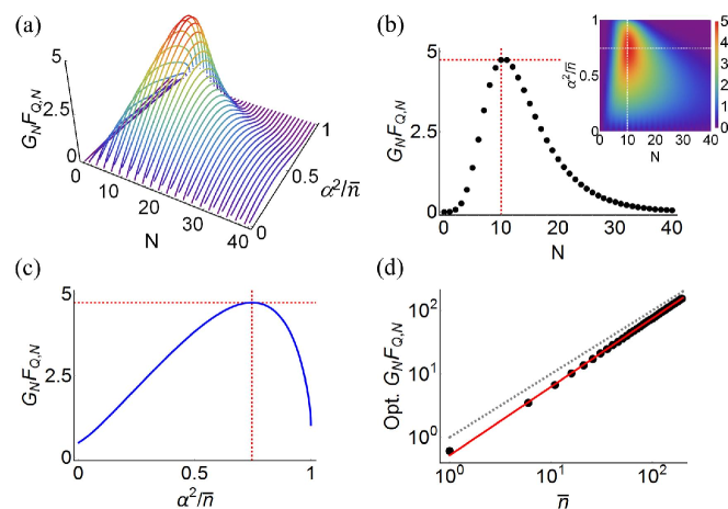
Indeed, the generated state under postselection cannot improve the ultimate precision for estimating a single parameter Combes ; Pang ; Haine , since the CFI is weighted by the generation probability, i.e., $G_{N}F_{N}(\varphi)$, where $F_{N}(\varphi)=F_{Q,N}$ has been given by Eq. (4). As depicted by Fig. 2, we find that for a given $\bar{n}=8$, the weighted CFI or the QFI $G_{N}F_{Q,N}$ reaches its maximum at $N=10$ and $\alpha^{2}/\bar{n}=0.75$. This means that the $10$-photon detection events give the best precision when the MZI is fed by an optimal input state with $\alpha^{2}=6$ and $\sinh^{2}\xi=2$. For each a given $\bar{n}\in[1,200]$, we optimize $G_{N}F_{Q,N}$ with respect to $\{N,\alpha^{2}\}$. From Fig. 2(d), one can see that the maximum of $G_{N}F_{Q,N}$ can be well fitted by $0.52\bar{n}^{1.08}$, which cannot surpass the classical limit as long as $\bar{n}<10^{3}$. To enlarge the CFI and hence the ultimate precision, all the detection events have to be taken into account (see below).

Figure 2: For a given $\bar{n}$, the QFI $G_{N}F_{Q,N}$ reaches its maximum at certain values of $N$ and $\alpha^{2}/\bar{n}$. (a)-(c) The 3D plot of the QFI for $\bar{n}=8$ and its 2D cross-sections at $\alpha^{2}/\bar{n}=0.75$ and $N=10$ (marked by the dashed white lines in the inset). (d) Optimal values of the QFI for each a given $\bar{n}\in[1,200]$, which, fitted by $0.52\bar{n}^{1.08}$ (the red solid), cannot surpass the classical limit (the dashed line) as long as $\bar{n}<10^{3}$.

III Scaling of the total Fisher information

Photon counting over a continuous-variable state, there are in general infinite number of the outcomes and all the $N$-photon detection events $\{N_{a},N_{b}\}$ contribute to the CFI. However, the photon number-resolving detector to data is usually limited by a finite number resolution Smerzi07 ; Kardynal , i.e., $N_{a}+N_{b}=N\leq$ $N_{\mathrm{res}}$, where $N_{\mathrm{res}}$ is the upper threshold of a single detector. Taking all the detectable events into account, the total CFI is given by

$$F(\varphi)=\sum_{N=0}^{N_{\mathrm{res}}}\sum_{\mu=-N/2}^{+N/2}\frac{\left[\partial P(N,\mu|\varphi)/\partial\varphi\right]^{2}}{P(N,\mu|\varphi)}=\sum_{N=0}^{N_{\mathrm{res}}}G_{N}F_{N}(\varphi),$$ (5)

where $P(N,\mu|\varphi)=|\langle J,\mu|\exp(-i\varphi J_{y})|\psi_{\mathrm{in}}\rangle|^{2}$ denote the probabilities for detecting the photon-counting events $\{N_{a},N_{b}\}$. In the last result, we have reexpressed the input state as $|\psi_{\mathrm{in}}\rangle=\sum_{N}\sqrt{G_{N}}|\psi_{N}\rangle$ and therefore, $P(N,\mu|\varphi)=G_{N}P_{N}(\mu|\varphi)$, where $G_{N}$ is the generation probability of the $N$-photon state $|\psi_{N}\rangle$. From Eq. (5), one can easily see that the total CFI is a sum of each $N$-component contribution weighted by $G_{N}$. With only the $N$-photon detection events, the CFI is simply given by $G_{N}F_{N}(\varphi)$, as mentioned above.

For the phase-matched input state, we have shown that the CFI of each $N$-photon component equals to that of the QFI, i.e., $F_{N}(\varphi)=4\langle\tilde{\psi}_{N}|J_{y}^{2}|\tilde{\psi}_{N}\rangle=F_{Q,N}$, which in turn gives

$$F(\varphi)=\sum_{N=0}^{N_{\mathrm{res}}}G_{N}F_{Q,N}=4\sum_{N=0}^{N_{\mathrm{res}}}G_{N}\langle\tilde{\psi}_{N}|J_{y}^{2}|\tilde{\psi}_{N}\rangle=F_{Q},$$ (6)

where $F_{Q}$ denotes the total QFI. To see it clearly, let us consider the QFI in the limit of $N_{\mathrm{res}}=\infty$ (i.e., the exact perfect PNRDs). In this ideal case, the above result becomes

$$F^{\mathrm{(id)}}(\varphi)=4\sum_{N=0}^{\infty}G_{N}\langle\tilde{\psi}_{N}|J_{y}^{2}|\tilde{\psi}_{N}\rangle=4\langle\psi_{\mathrm{in}}|J_{y}^{2}|\psi_{\mathrm{in}}\rangle=F_{Q}^{\mathrm{(id)}},$$ (7)

where $F_{Q}^{\mathrm{(id)}}$ is indeed the QFI of the input state $|\psi_{\mathrm{in}}\rangle=|\alpha\rangle_{a}\otimes|\xi\rangle_{b}$, for which $\langle\psi_{\mathrm{in}}|J_{y}|\psi_{\mathrm{in}}\rangle=\mathrm{Im}\langle\psi_{\mathrm{in}}|a^{{\dagger}}b|\psi_{\mathrm{in}}\rangle=0$.

It should be pointed out that all the events $\{N_{a},N_{b}\}$ with $N_{a}+N_{b}>N_{\mathrm{res}}$ are undetectable and have been discarded in Eq. (5). However, if we treat them as an additional outcome, the total CFI becomes $F(\varphi)+[\partial P(\mathrm{add}|\varphi)/\partial\varphi]^{2}/P(\mathrm{add}|\varphi)$, where

$$P(\mathrm{add}|\varphi)=1-\sum_{N=0}^{N_{\mathrm{res}}}\sum_{\mu=-N/2}^{+N/2}P(N,\mu|\varphi).$$ (8)

For the perfect MZI considered here, the additional outcome contains no phase information as $P(\mathrm{add}|\varphi)=1-\sum_{N=0}^{N_{\mathrm{res}}}G_{N}$ and hence $\partial P(\mathrm{add}|\varphi)/\partial\varphi=0$. Therefore, Eq. (5) still works to quantify the ultimate estimation precision.

Previously, we have considered the photon counters with a large enough number resolution $N_{\mathrm{res}}$ ($\geq 5\bar{n}$) and found that the optimal input state contains more coherent light photons than that of the squeezed vacuum PLiu , rather than the commonly used optimal input state (i.e., $|\alpha|^{2}\approx\sinh^{2}|\xi|$). Here, we further consider the PNRDs with a low resolution threshold $N_{\mathrm{res}}\sim\bar{n}$. For brevity, we assume the two injected light fields with $\alpha,\xi\in\mathbb{R}$, for which the phase-matching condition is fulfilled and hence the CFI still equals to the QFI. Combining Eqs. (4) and (5), we first rewrite the exact result of the QFI (see the Appendix) as

$$F_{Q}=\sum_{N_{a}=0}^{N_{\mathrm{res}}}\sum_{N_{b}=0}^{N_{\mathrm{res}}-N_{a}}\left[N_{a}+\left(1+2N_{a}+\frac{2\alpha^{2}}{\tanh\xi}\right)N_{b}\right]\left(c_{N_{a}}s_{N_{b}}\right)^{2},$$ (9)

where $c_{n}$ and $s_{k}$ are real, as mentioned above. Next, we note that the photon number distribution of the squeezed vacuum is usually wider than that of the coherent state (see Fig. 1), so we obtain

$$\sum_{N_{a}=0}^{N_{\mathrm{res}}}\sum_{N_{b}=0}^{N_{\mathrm{res}}-N_{a}}N_{a}f(N_{b})\left(c_{N_{a}}s_{N_{b}}\right)^{2}\approx\sum_{N_{a}=0}^{\infty}N_{a}c_{N_{a}}^{2}\sum_{N_{b}=0}^{N_{\mathrm{res}}-\bar{n}_{a}}f(N_{b})s_{N_{b}}^{2}=\bar{n}_{a}\sum_{N_{b}=0}^{N_{\mathrm{res}}-\bar{n}_{a}}f(N_{b})s_{N_{b}}^{2}.$$

This is because for a large enough $N_{\mathrm{res}}$, the sum over $N_{a}$ is complete and thereby, $\bar{n}_{a}=\sum_{N_{a}=0}^{\infty}N_{a}c_{N_{a}}^{2}=\alpha^{2}$, being average photon number from the input port $a$. Therefore, we immediately obtain an approximate result of the QFI

$$F_{Q}\approx\bar{n}_{a}\sum_{N_{b}=0}^{N_{\mathrm{res}}-\bar{n}_{a}}s_{N_{b}}^{2}+\left(1+2\bar{n}_{a}+\frac{2\bar{n}_{a}}{\tanh\xi}\right)\sum_{N_{b}=0}^{N_{\mathrm{res}}-\bar{n}_{a}}N_{b}s_{N_{b}}^{2}.$$ (10)

To validate it, we consider the limit $N_{\mathrm{res}}=\infty$ and a finite $\bar{n}_{a}$ and obtain

$$F_{Q} \approx \bar{n}_{a}+\left(1+2\bar{n}_{a}+\frac{2\bar{n}_{a}}{\tanh\xi}\right)\bar{n}_{b}$$ (11)

$$= \bar{n}+2\bar{n}_{a}\bar{n}_{b}\left(1+\sqrt{1+\frac{1}{\bar{n}_{b}}}\right)=F_{Q}^{\mathrm{(id)}},$$

where $\bar{n}_{b}=\sum_{N_{b}=0}^{\infty}N_{b}s_{N_{b}}^{2}=\sinh^{2}(\xi)$ is the mean photon number from the port $b$, and $1/\tanh\xi=\sqrt{1+1/\bar{n}_{b}}$. Using the relation $2\bar{n}_{b}(1+\sqrt{1+1/\bar{n}_{b}})=\exp(2\xi)-1$, we further obtain the ideal result of the QFI $F_{Q}^{\mathrm{(id)}}=\alpha^{2}\exp(2\xi)+\sinh^{2}(\xi)$, in agreement with previous result Smerzi08 . When the two input fields are phase matched and are optimally chosen (i.e., $\bar{n}_{a}\approx\bar{n}_{b}\approx\bar{n}/2$) Smerzi08 ; Liu ; Lang , it has been shown that $F_{Q}^{\mathrm{(id)}}$ can reach the Heisenberg scaling $\sim O(\bar{n}^{2})$. To saturate it, the exactly perfect PNRDs are needed in the photon counting measurements Seshadreesan .

For the imperfect PNRDs with a finite number resolution, we now calculate analytical result of the QFI. To this end, we first simplify Eq. (10) as

$$F_{Q}\approx F_{Q}^{\mathrm{(id)}}\left(1-\frac{1}{\bar{n}_{b}}\sum_{N_{b}=N_{\mathrm{res}}-\bar{n}_{a}+1}^{\infty}N_{b}s_{N_{b}}^{2}\right),$$ (12)

where we have used the completeness of $|\xi\rangle$, the relation $(1+2\bar{n}_{a}+2\bar{n}_{a}/\tanh\xi)=(F_{Q}^{\mathrm{(id)}}-\bar{n}_{a})/\bar{n}_{b}$, and neglected the terms $\sim O(\bar{n}_{a})$. Next, we use Stirling’s formula and replace the sum by an integral, namely

$$F_{Q}\!\! \approx \!\!F_{Q}^{\mathrm{(id)}}\left[1-\frac{1}{\bar{n}_{b}}\int_{N_{\mathrm{res}}-\bar{n}_{a}+1}^{\infty}\frac{N_{b}}{2}p(N_{b})dN_{b}\right]$$ (13)

$$= \!\!F_{Q}^{\mathrm{(id)}}\left[1-\sqrt{\frac{\bar{n}_{b}}{1+\bar{n}_{b}}}\frac{1}{(\bar{n}_{b}B)^{3/2}}\left(\mathrm{erfc}\left(A\right)+\frac{2A}{\sqrt{\pi}}e^{-A^{2}}\right)\right],$$

where, in the first step, $p(N_{b})$ denotes the photon number distribution of the squeezed vacuum, which can be well approximated by Eq. (1). In the second step, $\mathrm{erfc}(A)$ denotes a complementary error function, $B\equiv\log(1+1/\bar{n}_{b})$, and

$$A\equiv\sqrt{\frac{N_{\mathrm{res}}-\bar{n}_{a}+1}{2}B}.$$ (14)

Clearly, the total QFI depends upon three variables $\{N_{\mathrm{res}},\bar{n}_{a},\bar{n}_{b}\}$. For given values of $N_{\mathrm{res}}$ and $\bar{n}$, one can maximize $F_{Q}$ with respect to $\bar{n}_{a}$ (or $\bar{n}_{b}$) to obtain the optimal input state and the maximum of the QFI. For instance, let us consider the limit $N_{\mathrm{res}}\rightarrow\infty$ and hence $A\rightarrow\infty$, for which both $\mathrm{erfc}(A)$ and $A\exp(-A^{2})$ are vanishing. Therefore, we immediately obtain the ideal result of the QFI. The optimal input state can be obtained by maximizing Eq. (11), which can be approximated as

$$F_{Q}^{\mathrm{(id)}}\approx\bar{n}+\bar{n}_{a}\left(4\bar{n}_{b}+1\right),$$

where $\sqrt{1+1/\bar{n}_{b}}\approx 1+1/(2\bar{n}_{b})$ as $\bar{n}_{b}\gg 1$. With a constraint on $\bar{n}$ ($\gg 1$), it is easy to find that $F_{Q}^{\mathrm{(id)}}$ reaches its maximum $\bar{n}(\bar{n}+3/2)$ at $\bar{n}_{b}=\bar{n}/2-1/8$, in agreement with previous results Smerzi08 ; Liu ; Lang .

Numerically, the optimal input state can be determined by maximizing Eqs. (9) and (11) with respect to $\alpha^{2}$ (i.e., $\bar{n}_{a}$) for given $\bar{n}$ and $N_{\mathrm{res}}$. As depicted in Fig. 3(a), we choose a fixed mean photon number $\bar{n}=10$ and $N_{\mathrm{res}}=\bar{n}$ (the diamonds), $2\bar{n}$ (the squares), $5\bar{n}$ (the circles), and $\infty$ (the dash-dotted line). The solid lines are obtained from Eq. (13), which works well to predict the optimal value of $\alpha^{2}$, denoted hereinafter by $\alpha_{\mathrm{opt}}^{2}$ (see the arrows). In Fig. 3(b) and (c), we plot $\alpha_{\mathrm{opt}}^{2}/\bar{n}$ and $F_{Q,\mathrm{opt}}=F_{Q}(\alpha_{\mathrm{opt}}^{2},N_{\mathrm{res}})$ for each a given value of $\bar{n}\in[1,100]$, where the values of $N_{\mathrm{res}}$ are taken the same to Fig. 3(a). When $N_{\mathrm{res}}>\bar{n}\gg 1$, the analytical results of $\alpha_{\mathrm{opt}}^{2}/\bar{n}$ (the solid lines) show good agreement with the numerical results.

Figure 3: For given values of $\bar{n}$ and $N_{\mathrm{res}}$, the total QFI $F_{Q}$ reaches its maximum at a certain value of $\alpha^{2}/\bar{n}$ (see the arrows). (a) The total QFI $F_{Q}$ as a function of $\alpha^{2}/\bar{n}$ for $\bar{n}=10$ and $N_{\mathrm{res}}=\bar{n}$ (Diamonds), $2\bar{n}$ (Squares), $5\bar{n}$ (Circles), and $\infty$ (Black dash-dotted line). (b) and (c) The optimal value of $\alpha^{2}/\bar{n}$ and the associated QFI $F_{Q,\mathrm{opt}}$ for each a given $\bar{n}\in[1,100]$, where $N_{\mathrm{res}}$ are chosen the same with (a). The solid lines are analytical results that obtained from Eq. (13). The red dashed line in (c) is given by Eq. (17). The shaded area in (c): A region that below the classical limit $F_{Q}=\bar{n}$.

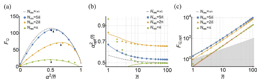
In Figure 3(c), one can see that $F_{Q,\mathrm{opt}}$ scales as $\bar{n}^{2}$ even for the photon counters with a relatively small number resolution (e.g., $N_{\mathrm{res}}\sim\bar{n}$). To confirm it, we assume the upper threshold of the number resolution $N_{\mathrm{res}}=\bar{n}$ with integer $\bar{n}$’s, and calculate analytical result of $F_{Q,\mathrm{opt}}$. As shown in Fig. 3(b), the maximum of the QFI appears at $\alpha_{\mathrm{opt}}^{2}/\bar{n}\rightarrow 1/2$ as $N_{\mathrm{res}}=\bar{n}\gg 1$, indicating that the optimal input state is the same to the ideal case (i.e., $\bar{n}_{a}\approx\bar{n}_{b}\approx\bar{n}/2$). Inserting $N_{\mathrm{res}}=\bar{n}$ and $\bar{n}_{a}=\bar{n}-\bar{n}_{b}$ into Eq. (13), one can note that the QFI is a function of $\bar{n}_{b}$ for each a given $\bar{n}$. Therefore, the term $\mathrm{erfc}\left(A\right)$ can be expanded in series of $1/\bar{n}_{b}$,

$$\mathrm{erfc}\left(A\right)=\mathrm{erfc}\left(\frac{1}{\sqrt{2}}\right)-\frac{\bar{n}_{b}^{-1}}{2\sqrt{2e\pi}}+O(\bar{n}_{b}^{-2}),\text{ \ \ \ }$$ (15)

and similarly,

$$\frac{2A}{\sqrt{\pi}}e^{-A^{2}}=\sqrt{\frac{2}{e\pi}}-\frac{\bar{n}_{b}^{-2}}{8\sqrt{2e\pi}}+O(\bar{n}_{b}^{-3}).$$ (16)

When $\bar{n}_{b}\gg 1$, only the leading term dominates in the above results, and $\bar{n}_{b}B\approx 1$, so we obtain

$$F_{Q}\approx F_{Q}^{\mathrm{(id)}}\left[1-\mathrm{erfc}\left(\frac{1}{\sqrt{2}}\right)-\sqrt{\frac{2}{e\pi}}\right]\approx 0.2\bar{n}^{2},$$ (17)

where $F_{Q}^{\mathrm{(id)}}\approx\bar{n}^{2}$ at $\bar{n}_{b}\approx\bar{n}/2$, as mentioned above. This scaling shows a good agreement with the numerical result (the diamonds); see Fig. 3(c). Furthermore, one can see that the estimation precision can surpass the classical limit as long as $N_{\mathrm{res}}=\bar{n}>10$.

Finally, it should be mentioned that the Heisenberg limit of phase sensitivity is also attainable using coherent $\otimes$ Fock state as the input Pezze , and a product of two squeezed-vacuum states Lang2 . To achieve such a estimation precision, we show here that it is also important to consider the influence of a finite number resolution of photon-counting detectors.

IV Conclusion

In summary, we have investigated the role of number-resolution-limited photon counters in the squeezed-state interferometer. Purely with a finite-$N$ detection events, we find that the CFI equals to the QFI and is weighted by the generation probability of the $N$-photon states under postselection. We numerically show that the maximum of the CFI or equivalently the QFI can be well fitted as $0.52\bar{n}^{1.08}$, which is slightly worse than the classical limit as long as $\bar{n}<10^{3}$. The ultimate precision can be improved if all the $N$-photon detection events are taken into account. For the PNRDs with a finite number resolution, the QFI is a sum of different $N$-photon components with $N\leq N_{\mathrm{res}}$, which can be approximated by a simple formula. When $N_{\mathrm{res}}\sim\bar{n}$, our analytical result shows that maximum of the total QFI scales as $0.2\bar{n}^{2}$, indicating that the optimal estimation precision can beat the classical limit for large enough $\bar{n}$.

Appendix A The Fisher information under the phase-matching condition

We first consider the two light fields with real amplitudes (i.e., $\alpha$, $\xi\in\mathbb{R}$), and calculate the QFI of the $N$-photon state under postselction. In Fock basis, it is given by Eq. (2) for the phases $\theta_{a}=\theta_{b}=0$,

$$|\tilde{\psi}_{N}\rangle=\frac{1}{\sqrt{G_{N}}}\sum_{k=0}^{N}c_{N-k}(0)s_{k}(0)|N-k\rangle_{a}\otimes|k\rangle_{b},$$ (18)

where the subscripts $a$ and $b$ represent two input ports or two orthogonally polarized light modes. The probability amplitudes of the two fields are given by

$$c_{n}(\theta_{a})\equiv\langle n|\alpha\rangle_{a}=e^{-|\alpha|^{2}/2}\frac{|\alpha|^{n}e^{in\theta_{a}}}{\sqrt{n!}},$$ (19)

and

$$s_{k}(\theta_{b})\equiv\langle k|\xi\rangle_{b}=\frac{H_{k}(0)}{\sqrt{k!\cosh|\xi|}}\left(e^{i\theta_{b}}\frac{\tanh|\xi|}{2}\right)^{k/2},$$ (20)

where $H_{2k}(0)=(-1)^{k}(2k)!/k!$ and $H_{2k+1}(0)=0$, are the Hermite polynomials $H_{k}(x)$ at $x=0$.

Next, we treat $|\tilde{\psi}_{N}\rangle$ as the input state and calculate the QFI of the output $\exp(-i\varphi J_{y})|\tilde{\psi}_{N}\rangle$. For the pure state, the QFI is simply given by $F_{Q,N}=4(\langle\tilde{\psi}_{N}|J_{y}^{2}|\tilde{\psi}_{N}\rangle-\langle\tilde{\psi}_{N}|J_{y}|\tilde{\psi}_{N}\rangle^{2})$ Braunstein ; Luo ; Smerzi09 ; Giovannetti , where $J_{y}=(a^{{\dagger}}b-b^{{\dagger}}a)/(2i)$ and $\langle\tilde{\psi}_{N}|J_{y}|\tilde{\psi}_{N}\rangle=0$, since $|\tilde{\psi}_{N}\rangle$ contains only even number of photons in the mode $b$. Therefore, we obtain

$$F_{Q,N}=4\langle\tilde{\psi}_{N}|J_{y}^{2}|\tilde{\psi}_{N}\rangle=\langle(2a^{{\dagger}}ab^{{\dagger}}b+a^{{\dagger}}a+b^{{\dagger}}b)\rangle-\langle(a^{{\dagger}2}b^{2}+H.c.)\rangle,$$ (21)

where $H.c.$ denotes the Hermitian conjugate and the expectation values are taken with respect to $|\tilde{\psi}_{N}\rangle$. It is easy to obtain the first term of Eq. (21),

$$\langle(2a^{{\dagger}}ab^{{\dagger}}b+a^{{\dagger}}a+b^{{\dagger}}b)\rangle=\frac{1}{G_{N}}\sum_{k=0}^{N}\left[2\left(N-k\right)k+N\right]\left(c_{N-k}s_{k}\right)^{2}.$$ (22)

The second term of Eq. (21) can be obtained by calculating

$$\langle a^{{\dagger}2}b^{2}\rangle=\frac{1}{G_{N}}\sum_{k=2}^{N}c_{N-k+2}s_{k-2}c_{N-k}s_{k}\sqrt{k\left(k-1\right)\left(N-k+1\right)\left(N-k+2\right)},$$ (23)

which is real. Using the relations

$$c_{N-k+2} = c_{N-k}\frac{\alpha^{2}}{\sqrt{(N-k+2)(N-k+1)}},$$

$$s_{k-2} = s_{k}\frac{k}{\sqrt{k(k-1)}}\left(-\frac{1}{\tanh\xi}\right),$$

we further obtain

$$\langle(a^{{\dagger}2}b^{2}+H.c.)\rangle=-\frac{1}{G_{N}}\sum_{k=0}^{N}\frac{2\alpha^{2}k}{\tanh\xi}\left(c_{N-k}s_{k}\right)^{2},$$ (24)

where, in the sum over $k$, we artificially include two vanishing terms for $k=0$, $1$. Combining Eqs. (22) and (24), we obtain the QFI of the $N$-photon state under the postselection; see Eq. (4) in main text.

Finally, one can note that the above results hold for the two light field with the complex amplitudes $\alpha$, $\xi$, provided that they are phase matched, i.e., $\cos(\theta_{b}-2\theta_{a})=+1$. Under this condition, the $N$-photon state can be expressed as $|\psi_{N}\rangle=\exp(iN\theta_{a})|\tilde{\psi}_{N}\rangle$, which $\theta_{a}$ is an arbitrary phase of the coherent light. Similar to Eq. (4), the CFI of each $N$-photon state is the same with that of the QFI. Furthermore, from Eqs. (5) and (6), one can see that the total CFI (or equivalently, the QFI) is a sum of each $N$-photon component, so we obtain

$$F_{Q}=\sum_{N=0}^{N_{\mathrm{res}}}G_{N}F_{Q,N}=\sum_{N=0}^{N_{\mathrm{res}}}\sum_{k=0}^{N}\left[2\left(N-k\right)k+N+\frac{2\alpha^{2}k}{\tanh\xi}\right]\left(c_{N-k}s_{k}\right)^{2}.$$ (25)

Setting $k=N_{b}$ and $N-k=N_{a}$, we further obtain the exact result of the QFI as Eq. (9) in main text.

References

- (1) C. W. Helstrom, Quantum Detection and Estimation Theory (Academic, New York, 1976).
- (2) S. M. Kay, Fundamentals of Statistical Signal Processing: Estimation Theory (Prentice-Hall, Englewood Cliffs, NJ, 1993).
- (3) S. L. Braunstein and C. M. Caves, Phys. Rev. Lett. 72, 3439 (1994); S. L. Braunstein, C. M. Caves, and G. J. Milburn, Ann. Phys. (N.Y.) 247, 135 (1996).
- (4) S. Luo, Phys. Rev. Lett. 91, 180403 (2003).
- (5) L. Pezzé and A. Smerzi, Phys. Rev. Lett. 102, 100401 (2009); F. Benatti, R. Floreanini, and U. Marzolino, Ann. Phys. 325, 924 (2010).
- (6) V. Giovannetti, S. Lloyd , and L. Maccone, Nat. Photonics 5, 222 (2011).
- (7) C. M. Caves, Phys. Rev. D 23, 1693 (1981).
- (8) J. Aasi, J. Abadie, B. Abbott et al., Nat. Photonics 7, 613 (2013).
- (9) I. Kruse, K. Lange, J. Peise, B. Lücke, L. Pezzé, J. Arlt, W. Ertmer, C. Lisdat, L. Santos, A. Smerzi, and C. Klempt, Phys. Rev. Lett. 117, 143004 (2016).
- (10) J. Peise, B. Lücke, L. Pezzé, F. Deuretzbacher, W. Ertmer, J. Arlt, A. Smerzi, L. Santos, and C. Klempt, Nat. Comm. 6, 1038 (2015).
- (11) L. Pezzé and A. Smerzi, Phys. Rev. Lett. 100, 073601 (2008).
- (12) J. Liu, X. Jing, and X. Wang, Phys. Rev. A 88, 042316 (2013).
- (13) M. D. Lang and C. M. Caves, Phys. Rev. Lett. 111, 173601 (2013).
- (14) K. P. Seshadreesan, P. M. Anisimov, H. Lee, and J. P. Dowling, New J. Phys. 13, 083026 (2011).
- (15) L. Pezzé, A. Smerzi, G. Khoury, J. F. Hodelin, and D. Bouwmeester, Phys. Rev. Lett. 99, 223602 (2007).
- (16) B. E. Kardynal, Z. L. Yuan, and A. J. Shields, Nat. Photonics 2, 425 (2008).
- (17) R. E. Slusher, L. W. Hollberg, B. Yurke, J. C. Mertz, and J. F. Valley, Phys. Rev. Lett. 55, 2409 (1985).
- (18) L.-A. Wu, H. J. Kimble, J. L. Hall, and H. Wu, Phys. Rev. Lett. 57, 2520 (1986); L.-A. Wu, M. Xiao, and H. J. Kimble, J. Opt. Soc. Am. B 4, 1465 (1987).
- (19) R. E. Slusher, P. Grangier, A. LaPorta, B. Yurke, and M. J. Potasek, Phys. Rev. Lett. 59, 2566 (1987).
- (20) G. Breitenbach, S. Schiller, and J. Mlynek, Nature 387, 471 (1997).
- (21) H. Vahlbruch, M. Mehmet, S. Chelkowski, B. Hage, A. Franzen, N. Lastzka, S. Goßler, K. Danzmann, and R. Schnabel, Phys. Rev. Lett. 100, 033602 (2008); H. Vahlbruch, M. Mehmet, K. Danzmann, and R. Schnabel, Phys. Rev. Lett. 117, 110801 (2016).
- (22) J. P. Dowling, Contemp. Phys. 49, 125 (2008); J. P. Dowling and K. P. Seshadreesan, J. Lightwave Technology 33, 2359 (2015).
- (23) J. Ma, X. Wang, C. P. Sun, and F. Nori, Phys. Rep. 509, 89 (2011).
- (24) Y. R. Zhang, G. R. Jin, J. P. Cao, W. M. Liu, and H. Fan, J. Phys. A: Math. Theor. 46, 035302 (2013).
- (25) G. Tóth and I. Apellaniz, J. Phys. A: Math. Theor. 47, 424006 (2014).
- (26) Q. S. Tan, J. Q. Liao, X. G. Wang, and F. Nori, Phys. Rev. A 89, 053822 (2014).
- (27) J. C. F. Matthews, X. Q. Zhou, H. Cable, P. J. Shadbolt, D. J. Saunders, G. A. Durkin, G. J. Pryde, and J. L. O’Brien, NPJ Quantum Information 2, 16023 (2016).
- (28) L. Pezzé, A. Smerzi, M. K. Oberthaler, R. Schmied, and P. Treutlein, arXiv:1609.01609 [quant-ph].
- (29) R. Demkowicz-Dobrzański, U. Dorner, B. J. Smith, J. S. Lundeen, W. Wasilewski, K. Banaszek, and I. A. Walmsley, Phys. Rev. A 80, 013825 (2009); U. Dorner, R. Demkowicz-Dobrzański, B. J. Smith, J. S. Lundeen, W. Wasilewski, K. Banaszek, and I. A. Walmsley, Phys. Rev. Lett. 102, 040403 (2009).
- (30) J. Joo, W. J. Munro, and T. P. Spiller, Phys. Rev. Lett. 107, 083601 (2011).
- (31) Y. M. Zhang, X. W. Li, W. Yang, and G. R. Jin, Phys. Rev. A 88, 043832 (2013).
- (32) P. A. Knott, W. J. Munro, and J. A. Dunningham, Phys. Rev. A 89, 053812 (2014).
- (33) A. Al-Qasimi and D. F. V. James, Opt. Lett. 34, 268 (2009).
- (34) B. Teklu, M. G. Genoni, S. Olivares, and M. G. A. Paris, Phys. Scr. T140, 014062 (2010).
- (35) Y. C. Liu, G. R. Jin, and L. You, Phys. Rev. A 82, 045601 (2010).
- (36) D. Brivio, S. Cialdi, S. Vezzoli, B. T. Gebrehiwot, M. G. Genoni, S. Olivares, and M. G. A. Paris, Phys. Rev. A 81, 012305 (2010).
- (37) M. G. Genoni, S. Olivares, and M. G. A. Paris, Phys. Rev. Lett. 106, 153603 (2011).
- (38) M. G. Genoni, S. Olivares, D. Brivio, S. Cialdi, D. Cipriani, A. Santamato, S. Vezzoli, and M. G. A. Paris, Phys. Rev. A 85, 043817 (2012).
- (39) B. M. Escher, L. Davidovich, N. Zagury, and R. L. de Matos Filho, Phys. Rev. Lett. 109, 190404 (2012).
- (40) W. Zhong, Z. Sun, J. Ma, X. Wang, and F. Nori, Phys. Rev. A 87, 022337 (2013).
- (41) B. Roy Bardhan, K. Jiang, and J. P. Dowling, Phys. Rev. A 88, 023857 (2013).
- (42) X. M. Feng, G. R. Jin, and W. Yang, Phys. Rev. A 90, 013807 (2014).
- (43) M. Zwierz and H. M. Wiseman, Phys. Rev. A 89, 022107 (2014).
- (44) Y. Gao and R. M. Wang, Phys. Rev. A 93, 013809 (2016).
- (45) B. Calkins, P. L. Mennea, A. E. Lita, B. J. Metcalf, W. S. Kolthammer, A. Lamas-Linares, J. B. Spring, P. C. Humphreys, R. P. Mirin, J. C. Gates, P. G. R. Smith, I. A. Walmsley, T. Gerrits, and S. W. Nam, Opt. Express 21, 22657 (2013).
- (46) P. Liu, P. Wang, W. Yang, G. R. Jin, and C. P. Sun, Phys. Rev. A 95, 023824 (2017).
- (47) I. Afek, O. Ambar, and Y. Silberberg, Science 328, 879 (2010).
- (48) H. F. Hofmann and T. Ono, Phys. Rev. A 76, 031806(R) (2007); T. Ono and H. F. Hofmann, Phys. Rev. A 81, 033819 (2010).
- (49) J. Combes, C. Ferrie, Z. Jiang, and C. M. Caves, Phys. Rev. A 89, 052117 (2014).
- (50) S. Pang and T. A. Brun, Phys. Rev. Lett. 115, 120401 (2015).
- (51) S. A. Haine, S. S. Szigeti, M. D. Lang, and C. M. Caves, Phys. Rev. A 91, 041802 (2015).
- (52) C. C. Gerry and P. L. Knight, Introductory Quantum Optics (Cambridge University Press, Cambridge, England, 2005).
- (53) L. Pezzé and A. Smerzi, Phys. Rev. Lett. 110, 163604 (2013).
- (54) M. D. Lang and C. M. Caves, Phys. Rev. A 90, 025802 (2014).