SILVERRUSH. VII. Subaru/HSC Identifications of 42 Protocluster Candidates at $z\sim 6-7$ with the Spectroscopic Redshifts up to $z=6.574$:
Implications for Cosmic Reionization

Abstract

We report fourteen and twenty-eight protocluster candidates at $z=5.7$ and $6.6$ over 14 and 19 deg² areas, respectively, selected from 2,230 (259) Ly$\alpha$ emitters (LAEs) photometrically (spectroscopically) identified with Subaru/Hyper Suprime-Cam (HSC) deep images (Keck, Subaru, and Magellan spectra and the literature data). Six out of the 42 protocluster candidates include $1-12$ spectroscopically confirmed LAEs at redshifts up to $z=6.574$. By the comparisons with the cosmological Ly$\alpha$ radiative transfer (RT) model reproducing LAEs with the reionization effects, we find that more than a half of these protocluster candidates are progenitors of the present-day clusters with a mass of $\gtrsim 10^{14}M_{\odot}$. We then investigate the correlation between LAE overdensity $\delta$ and Ly$\alpha$ rest-frame equivalent width $EW_{\rm Ly\alpha}^{\rm rest}$, because the cosmological Ly$\alpha$ RT model suggests that a slope of $EW_{\rm Ly\alpha}^{\rm rest}$-$\delta$ relation is steepened towards the epoch of cosmic reionization (EoR), due to the existence of the ionized bubbles around galaxy overdensities easing the escape of Ly$\alpha$ emission from the partly neutral intergalactic medium (IGM). The available HSC data suggest that the slope of the $EW_{\rm Ly\alpha}^{\rm rest}$-$\delta$ correlation does not evolve from the post-reionization epoch $z=5.7$ to the EoR $z=6.6$ beyond the moderately large statistical errors. There is a possibility that we would detect the evolution of the $EW^{\rm rest}_{\rm Ly\alpha}$ - $\delta$ relation from $z=5.7$ to $7.3$ by the upcoming HSC observations providing large samples of LAEs at $z=6.6-7.3$.

1. Introduction

Studying the physical process of cosmic reionization is one of the important subjects in astronomy today. It is suggested that cosmic reionization was completed by $z\sim 6$ by the studies of the Gunn-Peterson effect and the Ly$\alpha$ damping wing found in the continua of high-redshift QSOs and gamma-ray bursts (Fan et al. 2006; Bolton et al. 2011; Goto et al. 2011; Chornock et al. 2013; McGreer et al. 2015). Similarly, Ly$\alpha$ emission in high-redshift galaxies is used to investigate the ionization state of the intergalactic medium (IGM), because the Ly$\alpha$ damping wing of HI gas in the IGM attenuates Ly$\alpha$ photons from Ly$\alpha$ emitters (LAEs). Recently, Konno et al. (2017) and Ouchi et al. (2017) have constrained the neutral hydrogen fraction of the IGM to be $x_{\rm HI}\simeq 0.3\pm 0.2$ at $z=6.6$ from the evolution of the Ly$\alpha$ luminosity functions (LFs) and the angular correlation function based on the large samples of LAEs at $z\sim 6-7$ (see also Malhotra & Rhoads 2004; Kashikawa et al. 2006; Ouchi et al. 2008, 2010; Ota et al. 2010; Konno et al. 2014).

Despite the fact that the mean values of $x_{\rm HI}$ at $z\sim 6-7$ are constrained, it is still unclear what are the ionizing photon sources of cosmic reionization. Although there are several candidates for the major sources of cosmic reionization, many observations suggest that it is likely that star-forming galaxies are major sources of cosmic reionization (Robertson et al. 2015; Bouwens et al. 2015; Ishigaki et al. 2017). In this case, theoretical models predict that star-forming galaxies emitting ionizing photons from young massive stars would ionize the IGM around galaxies and that the ionized regions in the IGM are called ionized bubbles. Large ionized bubbles are expected to form in galaxy overdense regions, where many star-forming galaxies exist in a small volume of the universe (Furlanetto et al. 2006; Ono et al. 2012; Matthee et al. 2015; Ishigaki et al. 2016; Overzier 2016; Chiang et al. 2017). The cosmic reionization is expected to proceed from high- to low-density regions (see Iliev et al. 2006; Ono et al. 2012; Overzier 2016). This reionization process is called ’inside-out scenario’. On the other hand, if major sources of cosmic reionization are X-ray emitting objects like AGNs, the scenario may be different. Due to the longer mean-free path of X-ray photons than that of UV photons from galaxies and the slow hydrogen recombination rate in the low-density region, cosmic reionization would not proceed from high-density, but low-density regions (see Miralda-Escudé et al. 2000; Nakamoto et al. 2001; McQuinn 2012; Mesinger et al. 2013). The physical process of cosmic reionization is tightly related to the major ionizing sources of cosmic reionization. Because no definitive observational evidence of ionized bubbles is found to date, identifying signatures of ionized bubbles around galaxy overdense regions, if any, is key to testing the inside-out scenario of cosmic reionization.

There is another importance of observations of galaxy overdensities near the EoR. Standard structure formation models predict that a large fraction of high-$z$ galaxy overdense regions evolve into massive galaxy clusters at $z=0$. These galaxy overdense regions are called protoclusters. A protocluster is often defined as a structure expected to collapse into a galaxy cluster with a halo mass $M_{\rm h}>10^{14}\>\rm M_{\odot}$ (Chiang et al. 2013; Overzier 2016). Galaxy overdensities at the EoR would be examples of the first site of the galaxy cluster formation (e.g. Ishigaki et al. 2016).

Although the importances of high-$z$ galaxy overdensities are well recognized, only a few protoclusters at $z\gtrsim 6$ are reported, to date (Ouchi et al. 2005; Utsumi et al. 2010; Toshikawa et al. 2012, 2014; Franck & McGaugh 2016b, a; Chanchaiworawit et al. 2017; Toshikawa et al. 2017). It is popular that protoclusters are identified with the distributions of the continuum-selected galaxies including dropout galaxies. However, there is a difficulty to find protoclusters only with the continuum-selected galaxy samples due to the large redshift uncertainties of the continuum-selected galaxies. Instead, one can use LAEs to identify protoclusters or galaxy overdensities in general, exploiting a small redshift uncertainty of LAEs. Here we investigate the LAE distribution and overdensity to identify protocluster candidates, and to investigate the IGM ionization state around galaxy overdensities. The IGM ionization state is studied with the Ly$\alpha$ equivalent widths (EWs) of LAEs that depend on $x_{\rm HI}$ (Dijkstra et al. 2011, 2016; Jensen et al. 2014; Kakiichi et al. 2016). Having a number of galaxy overdensities, we statistically investigate protoclusters and the IGM ionization states.

In this paper, we identify protocluster candidates at $z=5.7$ and $6.6$ based on the LAE samples of Systematic Identification of LAEs for Visible Exploration and Reionization Research Using Subaru HSC (SILVERRUSH; Ouchi et al. 2017). SILVERRUSH is an on-going research project based on the Subaru/Hyper Suprime-Cam (HSC) Subaru Strategic Program (SSP; Aihara et al. 2017, Miyazaki et al. 2017, Komiyama et al. 2017, Furusawa et al. 2017). The SHILVERRUSH project papers show various properties of LAEs in the EoR, clustering (Ouchi et al. 2017), photometry (Shibuya et al. 2017a), spectroscopy (Shibuya et al. 2017b), Ly$\alpha$ LFs (Konno et al. 2017), the ISM properties (Harikane et al. 2017b), theoretical predictions (Inoue et al. 2018), and protoclusters (this work). This is the seventh publication in SILVERRUSH. SILVERRUSH is one of the twin programs devoted to scientific results on high redshift galaxies based on the HSC survey data. The other one is related to dropout galaxies, named Great Optically Luminous Dropout Research Using Subaru HSC (GOLDRUSH; Ono et al. 2017, Harikane et al. 2017a, Toshikawa et al. 2017). Because we intend to enlarge our LAE samples, we include the LAE samples made in Ouchi et al. (2008) and Ouchi et al. (2010), which are previously obtained with Subaru/Suprime-Cam (SC; Miyazaki et al. 2002; see also Iye et al. 2004). We describe our photometric LAE samples with HSC and SC in Section 2. In Sections 3 and 4, we explain our spectroscopic LAE data and theoretical models of Inoue et al. (2018), respectively. We present the list of protocluster candidates at $z=5.7$ and $6.6$, and show the 3-dimensional LAE distributions of protocluster candidates (Section 5). In Section 5, we also discuss the physical process of cosmic reionization with the LAE distributions.

Throughout this paper, we use a cosmological parameter set of $\Omega_{\mathrm{m}}=0.3$, $\Omega_{\mathrm{\Lambda}}=0.7$, $\Omega_{\mathrm{b}}=0.04$, and $H_{0}=70$ km s^-1 Mpc^-1. The magnitudes are in the AB system.

2. Data and Samples

2.1. Photometric Samples of HSC SSP Data

We calculate galaxy overdensity and identify protocluster candidates using photometric LAE samples of HSC SSP data. In our study, we use two-narrowband ($NB816$ and $NB921$) and five-broadband ($grizy$) imaging data, of the HSC SSP survey (Section 1) starting in March 2014. The HSC-SSP survey is an on-going program, for which 300 nights are allocated over 5 years. The HSC-SSP survey has three layers of the UltraDeep, Deep, and Wide, whose planned total survey areas are $\sim$ 4 $\rm deg^{2}$, $\sim$ 30 $\rm deg^{2}$, and $\sim 1400$ $\rm deg^{2}$, respectively. The narrowband data are taken only in the UltraDeep and Deep layers. We use early datasets of the HSC-SSP survey taken until April 2016. In these datasets, HSC SSP has obtained $NB816$ data in two fields of the UltraDeep layer, UD-SXDS and UD-COSMOS, and two fields of the Deep layer, D-ELAIS-N1, and D-DEEP2-3. The data of $NB921$ have been taken in two fields of the UltraDeep layer, UD-SXDS and UD-COSMOS, and three fields of the Deep layer, D-ELAIS-N1, D-DEEP2-3, and D-COSMOS. The $5\sigma$ limiting magnitudes of the HSC imaging data are typically $\simeq 25-25.5$ magnitudes in the narrowbands and $\simeq 26-27$ magnitudes in the broadbands (Table 1; see also Shibuya et al. 2017a). The total survey areas of the early datasets are 13.8 $\rm deg^{2}$ and 21.2 $\rm deg^{2}$ in the fields with the $NB816$ and $NB921$ data, respectively. The $NB816$ and $NB921$ data allow us to identify strong Ly$\alpha$ emission lines of LAEs redshifted to $z=5.726\pm 0.046$ and $z=6.580\pm 0.056$, respectively, where the redshift ranges are defined with the FWHMs of the narrowbands. The total survey volumes for the early datasets are $1.2\times 10^{7}{\rm\>Mpc}^{3}$ at $z=5.7$ and $1.9\times 10^{7}{\rm\>Mpc}^{3}$ at $z=6.6$. Note that these survey volumes are $\sim 2-50$ and $\sim 4-100$ times larger than those of previous studies for LAEs at $z=5.7$ (e.g. Ouchi et al. 2008; Santos et al. 2016) and $z=6.6$ (e.g. Ouchi et al. 2010; Kashikawa et al. 2011; Matthee et al. 2015), respectively.

The datasets are reduced by the HSC-SSP Collaboration with $\tt{hscPipe}$ (Bosch et al. 2017). $\tt{hscPipe}$ is a pipeline which is based on the Large Synoptic Survey Telescope (LSST) pipeline (Ivezic et al. 2008; Axelrod et al. 2010; Jurić et al. 2015). The astrometry and photometry of the datasets are calibrated based on the Panoramic Survey Telescope and Rapid Response System (Pan-STARRS) 1 imaging survey (Magnier et al. 2013; Schlafly et al. 2012; Tonry et al. 2012).

Our photometric samples of $z=5.7$ and $6.6$ LAEs are made with combinations of the narrowband color excess and the UV continuum break (Shibuya et al. 2017a). We apply color selection criteria which are similar to those of Ouchi et al. (2008) and Ouchi et al. (2010) who study $z=5.7$ and $6.6$ LAEs, respectively with SC. The color selection criteria to the objects in the HSC datasets are defined as

$$i-NB816\geq 1.2{\>\rm and\>}g>g_{3\sigma}{\>\rm and\>}$$ (1)

$$[(r{\leq}r_{3\sigma}{\>\rm and\>}r-i{\geq}1.0){\>{\rm or}\>}(r>r_{3\sigma})]$$

and

$$i-NB921\geq 1.0{\>\rm and\>}g>g_{3\sigma}{\>\rm and\>}r>r_{3\sigma}{\>\rm and\>}$$ (2)

$$[(z\leq z_{3\sigma}{\>\rm and\>}i-z\geq 1.0){\>\rm or\>}(z>z_{3\sigma})]$$

for $z=5.7$ and $6.6$ LAEs, respectively (see Shibuya et al. 2017a). We find 1,077 $z=5.7$ LAEs and 1,153 $z=6.6$ LAEs by photometry. Shibuya et al. (2017b) take spectra of 18 LAEs of the photometric samples, and confirm 13 LAEs at $z=5.7$ and $6.6$ by spectroscopy. Because the LAEs include faint sources that may not identify a signal with the depth of the spectroscopy, the contamination rate indicated by the spectroscopy is estimated to be $0-30$% in the $z=5.7$ and $6.6$ LAEs in the photometric samples.

Table 1HSC Imaging Data

Layer	Field	Area	$g$	$r$	$i$	$z$	$y$	$NB816$	$NB921$
(1)	(2)	$(3)$	$(4)$	$(5)$	$(6)$	$(7)$	$(8)$	$(9)$	(10)
UD	SXDS	1.928 (1.873)	26.9	26.4	26.3	25.6	24.9	25.5	25.5
UD	COSMOS	1.965 (1.999)	26.9	26.6	26.2	25.8	25.1	25.7	25.6
Deep	COSMOS	- (4.938)	26.5	26.1	26.0	25.5	24.7	-	25.3
Deep	ELAIS-N1	5.566 (5.599)	26.7	26.0	25.7	25.0	24.1	25.3	25.3
Deep	DEEP2-3	4.339 (3.100)	26.6	26.2	25.9	25.2	24.5	25.2	24.9

Note. — (1) Layer; (2) field; (3) effective area of the $NB816$ ($NB921$) image ($\rm deg^{2}$); (4)-(10) five sigma limiting magnitudes of the HSC $g$, $r$, $i$, $z$, $y$, $NB816$, and $NB921$ images in a circular aperture with a diameter of $1.^{\prime\prime}5$ (mag).

Table 2Photometric Samples of the $z=5.7$ and $6.6$ LAEs

		$z=5.7$			$z=6.6$
Layer	Field	$NB816$ Full	$NB816$ $<24.5$	$NB816$ $<25.0$	$NB921$ Full	$NB921$ $<24.5$	$NB921$ $<25.0$
(1)	(2)	(3)	(4)	(5)	(6)	(7)	(8)
UD	SXDS	224	83	164	58	21	43
UD	COSMOS	201	52	123	338	31	82
Deep	COSMOS	-a	-a	-a	244	91	196
Deep	ELAIS-N1	229	140	166	349	142	258
Deep	DEEP2-3	423	127	319	164	104	82
	Total	1077	402	772	1153	389	661

Note. — (1) Layer; (2) field; (3) number of the $z=5.7$ LAEs in the HSC photometric sample; (4)-(5) same as (3), but for $z=5.7$ LAEs that are brighter than 24.5 and 25.0 mag in the $NB816$ band; (6) number of the $z=6.6$ LAEs in the HSC photometric sample; (7)-(8) same as (6), but for $z=6.6$ LAEs that are brighter than 24.5 and 25.0 mag in the $NB921$ band. ^a The $NB816$ image is not taken in Deep COSMOS.

2.2. Photometric Samples of the SC Data

To select the spectroscopic targets of $z=5.7$ and $6.6$ LAEs, we use photometric samples of Ouchi et al. (2008) and Ouchi et al. (2010), respectively, in addition to the HSC LAE samples in Section 2.1. Ouchi et al. (2008) and Ouchi et al. (2010) have carried out narrowband imaging with SC in 2003 and 2005-2007, respectively. The total areas of the narrowband imaging are $\sim 1\>\rm deg^{2}$ and $\sim 0.9\>\rm deg^{2}$ for $NB816$ and $NB921$ images, respectively. Ouchi et al. (2008) and Ouchi et al. (2010) detect objects in each narrowband image with SExtractor (Bertin & Arnouts 1996), and obtain SC LAE samples with the color selection criteria similar to the equations (1) and (2) that are defined as

$$i^{{}^{\prime}}-NB816\geq 1.2{\>\rm and\>}B>B_{2\sigma}{\>\rm and\>}V>V_{2\sigma}{\>\rm and\>}$$

$$[(R{\leq}R_{2\sigma}{\>\rm and\>}R-i^{{}^{\prime}}{\geq}1.0){\>{\rm or}\>}(R>R_{2\sigma})]$$

and

$$z^{{}^{\prime}}-NB921\geq 1.0{\>\rm and\>}B>B_{2\sigma}{\>\rm and\>}V>V_{2\sigma}{\>\rm and\>}$$

$$[(z^{{}^{\prime}}\leq z^{{}^{\prime}}_{3\sigma}{\>\rm and\>}i^{{}^{\prime}}-z^{{}^{\prime}}\geq 1.3){\>\rm or\>}(z^{{}^{\prime}}>z^{{}^{\prime}}_{3\sigma})]$$

for $z=5.7$ and $6.6$ LAEs, respectively. Ouchi et al. (2008) and Ouchi et al. (2010) apply these selection criteria, and find 401 and 207 LAEs at $z=5.7$ and $6.6$, respectively.

Comparing the SC samples with the HSC samples, one can recognize that many LAEs in the SC samples are not included in the HSC samples. This is because the SC samples have faint LAEs down to the narrowband magnitudes of $\sim 26$ mag, while the depth of the HSC samples only reaches $\sim 25$ mag.

3. Spectroscopic Observations and Samples

We conduct spectroscopic observations for the HSC and SC LAE samples. The spectroscopic observations for the HSC samples are presented in Shibuya et al. (2017b). Here we explain our spectroscopy for the SC samples that were conducted in 2007-2010.

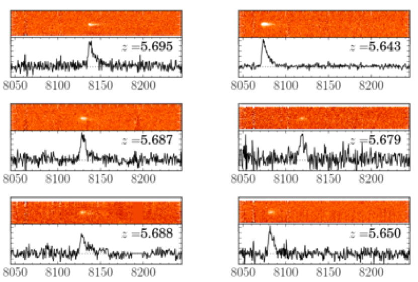
Figure 1.— Examples of the $z=5.7$ LAE spectra obtained by our Keck/DEIMOS observations. The two and one dimensional spectra are shown in the top and bottom subpanels, respectively, in each panel. The x-axis represents the observed wavelength.

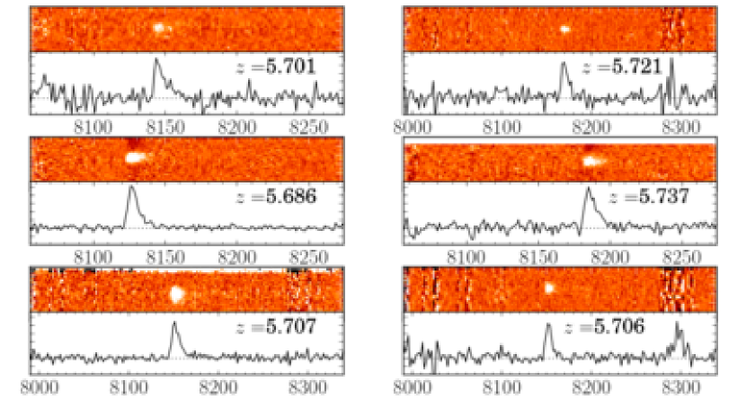
Figure 2.— Same as Figure 1, but for our Magellan/IMACS spectra of the $z=5.7$ LAEs.

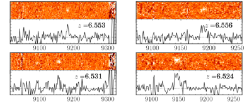
Figure 3.— Same as Figure 1, but for our Magellan/IMACS spectra of the $z=6.6$ LAEs.

Table 3Spectroscopic Observations

Layer	Field	Mask ID	Date	Total Exposure	${N_{\rm LAE}}$	Grism	$\rm CW$	Filter
(1)	(2)	(3)	(4)	(5)	(6)	(7)	(8)	(9)
Keck/DEIMOS
UD	SXDS	SXDS03	2010 Feb 11	3500	16	830	7900	OG550
Magellan/IMACS
UD	SXDS	sxds1_07	2007 Nov 12	15600	4	Gri-150-18.8	-	GG455
UD	SXDS	sxds3r07	2007 Nov 13-14	37800	15	Gri-150-18.8	-	OG570
UD	SXDS	sxds5s08	2008 Nov 29	15300	22	Gri-300-26.7	-	WB6300-9500
UD	SXDS	sxds3s08	2008 Nov 30	15300	27	Gri-300-26.7	-	WB6300-9500
UD	SXDS	sxds2a08	2008 Dec 1	16200	22	Gri-300-26.7	-	WB6300-9500
UD	SXDS	sxds4a08	2008 Dec 2	18000	12	Gri-300-26.7	-	WB6300-9500
UD	SXDS	sxds1u08	2008 Dec 18-19	25200	11	Gri-300-26.7	-	WB6300-9500
UD	SXDS	sxds3a09	2009 Oct 11	21600	26	Gri-300-26.7	-	WB6300-9500
UD	SXDS	sxds2a09	2009 Oct 12	15300	16	Gri-300-26.7	-	WB6300-9500
UD	SXDS	$\rm oct2008\_nb1190a^{a}$	2008 Oct 20-23	22500	9	Gri-300-26.7	-	WB6300-9500
UD	SXDS	$\rm oct2008\_nb1190b^{a}$	2008 Oct 20-23	18000	4	Gri-300-26.7	-	WB6300-9500
UD	SXDS	$\rm oct2008\_nb1190c^{a}$	2008 Oct 20-23	18000	8	Gri-300-26.7	-	WB6300-9500
UD	SXDS	$\rm oct2008\_nb1190d^{a}$	2008 Oct 20-23	18000	11	Gri-300-26.7	-	WB6300-9500
UD	SXDS	$\rm sep2009\_sxdsw1^{a}$	2009 Sep 19-20	12600	1	Gri-300-26.7	-	WB6300-9500
UD	SXDS	$\rm sep2009\_sxdsw2^{a}$	2009 Sep 19-20	12600	3	Gri-300-26.7	-	WB6300-9500
UD	COSMOS	cos01_08	2008 Nov 29 - Dec 2	21600	7	Gri-300-26.7	-	WB6300-9500
UD	COSMOS	cos02_08	2008 Dec 18-20	27900	5	Gri-300-26.7	-	WB6300-9500

Note. — (1) Layer; (2) field; (3) mask ID; (4) date of observations; (5) total exposure time (sec); (6) numbers of the observed LAEs; (7) disperser name; (8) central wavelength of the grating setting $(\rm\AA)$; (9) filter name. ^a See also Lee et al. (2012) and Momcheva et al. (2013).

3.1. Keck/DEIMOS Observation

We carried out spectroscopic follow-up observations for our $z=5.7$ LAEs with Deep Imaging Multi-Object Spectrograph (DEIMOS; Faber et al. 2003) on 2010 February 11. The sky was clear during the observations, and the seeing was $\sim 0^{\prime\prime}.5$. We observed 22 out of the 401 SC LAEs at $z=5.7$ (Ouchi et al. 2008) including very faint LAE candidates, and obtained 16 spectra in a good condition. During the observations, we took the standard stars G191B2B for the flux calibration. We used a mask with a slit width of $1^{\prime\prime}$, the OG550 filter, and the 830 lines ${\rm mm}^{-1}$ grating that is blazed at 8640 Å. The grating was tilted to be placed at a central wavelength of 7900 Å on the detectors. The spectral coverage and the spectral resolution were $4100-9400$Å and $\lambda/{\Delta}{\lambda}\simeq 2400$, respectively.

We perform the data reduction using the spec2d IDL pipeline developed by the DEEP2 Redshift Survey Team (Davis et al. 2003). The central wavelengths of Ly$\alpha$ emission were determined by Gaussian fitting. We detect 15 out of the 16 LAEs, and obtain Ly$\alpha$ line redshifts. The spectra of the example LAEs are shown in Figure 1.

3.2. Magellan/IMACS Observation

We conducted follow-up spectroscopy for 425 objects selected from the samples of $z=5.7$ and $z=6.6$ LAEs in Ouchi et al. (2008) and Ouchi et al. (2010), respectively. The observations were performed with the Inamori Magellan Areal Camera and Spectrograph (IMACS; Dressler et al. 2006) on the Magellan I Baade Telescope in 2007 November $12-14$, 2008 November 29 $-$ December 2, 2008 December $18-19$, and 2009 October $11-12$. We chose GG455 filter and Gri-150-18.8 grism on 2007 November 12. In 2007 November $13-14$, we change the filter from GG455 to OG570. For the rest of the IMACS observations, we used WB6300-9500 filter and gri-300-26.7 grism. The exposure time ranges from 15,300 s to 35,400 s with seeing sizes of $0^{\prime\prime}.5-0^{\prime\prime}.8$. We used a $0^{\prime\prime}.8$ slit width that gives a spectral resolution of $1,000-2,000$. We perform data reduction with the Carnegie Observatories System for MultiObject Spectroscopy (COSMOS) pipeline, and detect Ly$\alpha$ emission lines around 8160 Å (9210 Å ) for 130 (22) objects. Spectra of the example LAEs are shown in Figures 2-3.

3.3. Spectroscopic Samples and Catalogs

Adding to the SC spectroscopic sample of the LAEs confirmed with DEIMOS and IMACS in Sections 3.1 and 3.2 and the HSC spectroscopic sample of Shibuya et al. 2017b that includes LAEs in Ouchi et al. 2010, Sobral et al. 2015, and Hu et al. 2016, we use the redshift catalogs for the spectroscopically confirmed LAEs at $z=5.7$ ($6.6$) taken from Ouchi et al. (2005), Ouchi et al. (2008), Mallery et al. (2012), Chanchaiworawit et al. (2017), and Guzmán et al. (in preparation). We make unified spectroscopic catalogs of LAEs at $z=5.7$ and $6.6$ Tables 4 and 5, respectively.

Note that, again, there are many LAEs in the SC spectroscopic sample that are not included in the HSC photometric sample. This is because the HSC photometric sample includes bright LAEs only down to $\sim 25$ mag in a narrowband, while the SC samples (spectroscopic and photometric samples) have faint LAEs down to $\sim 26$ mag in a narrowband (Section 2.2). Because the selection of the SC (and HSC) spectroscopic sample is heterogeneous, we use the homogeneous photometric sample of HSC LAEs to find protocluster candidates. The unified catalogs (the SC and HSC spectroscopic samples) are referred to confirm the redshifts of protocluster candidates in Section 5.1.4.

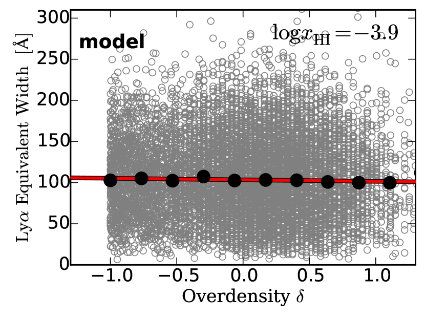
Figure 4.— $EW^{\rm rest}_{\rm Ly\alpha}$ as a function of $\delta$ at $\log_{\rm 10}{x_{\rm HI}}=-3.9$ (corresponding to $z=5.7$) in the model of Inoue et al. (2018). The values of $\delta$ and $EW^{\rm rest}_{\rm Ly\alpha}$ are shown with the gray open circles. The black filled circles and the bars indicate the median values and the error bars, respectively. The red line represents the best-fit linear function.

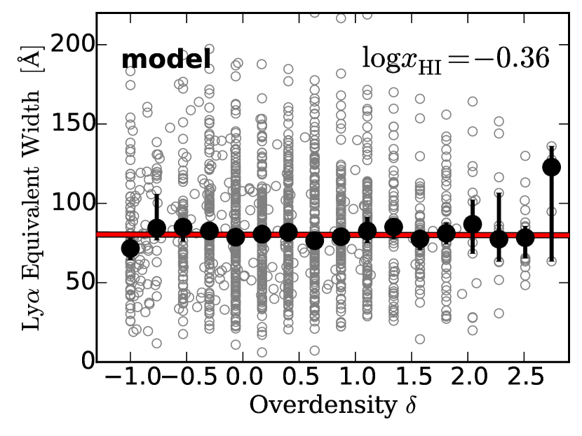
Figure 5.— Same as Figure 4, but for $\log_{\rm 10}{x_{\rm HI}}=-0.36$ (corresponding to $z=6.6$).

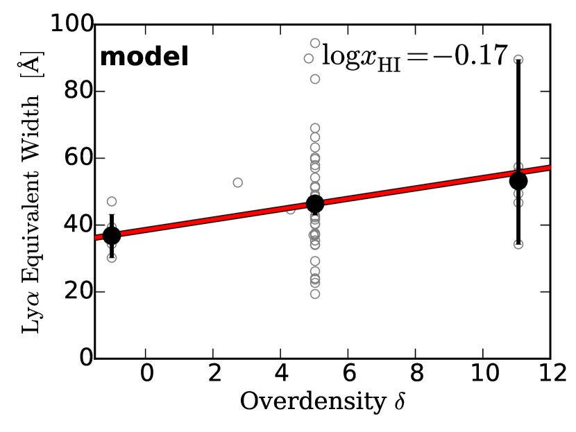
Figure 6.— Same as Figure 4, but for $\log_{\rm 10}{x_{\rm HI}}=-0.17$ (corresponding to $z=7.3$).

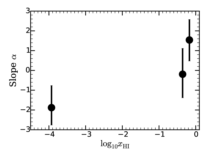
Figure 7.— Slope $\alpha$ of the $EW^{\rm rest}_{\rm Ly\alpha}$ - $\delta$ relation as a function of $x_{\rm HI}$ that is derived with the model of Inoue et al. (2018).

4. Theoretical Model

We compare our observational results with the cosmological simulation model of Inoue et al. (2018). Inoue et al. (2018) conduct the N-body simulations in a box size of $110h^{-1}$ comoving Mpc (cMpc) length with $512^{3}$ grids, which gives a spatial resolution of $214.8$ comoving kpc. Inoue et al. (2018) present models of three reionization histories depending on the ionizing emissivity of halos: $early$, $mid$, and $late$, all of which are consistent with the latest Thomson scattering optical depth measurement (Planck Collaboration et al. 2016). Here we adopt the $late$ model that explains the recent neutral hydrogen fraction measurements at $z\sim 6-7$. In the model, a total of $4096^{3}$ dark matter particles are used with a mass resolution of $7\times 10^{7}$ $M_{\odot}$. Inoue et al. (2018) perform numerical radiative transfer calculations to reproduce cosmic reionization.In this model, LAEs are created with the relation of the Ly$\alpha$ photon production rate and halo mass determined by the radiation hydrodynamics (RHD) galaxy formation simulation of Hasegawa et al. (in preparation). Inoue et al. (2018) assume

$$L_{\rm Ly\alpha,int}=10^{42}\times(1-e^{-10M_{\rm h,10}})\times{M_{\rm h,10}}^{1.1}\times 10^{\delta_{\rm Ly\alpha}}\>[\rm erg\>s^{-1}],$$ (5)

where more massive haloes produce more Ly$\alpha$ photons due to the higher star-forming rate (SFR). Here, ${M_{\rm h,10}}$ is the halo mass normalized by $10^{10}M_{\odot}$, and $\delta_{\rm Ly\alpha}$ represents the fluctuation of the Ly$\alpha$ photon production. The ISM Ly$\alpha$ escape fraction is defined as

$$f_{{\rm esc},\alpha}^{\rm ISM}=\exp(-\tau_{\rm\alpha}),$$ (6)

where $\tau_{\alpha}$ is the Ly$\alpha$ optical depth. Inoue et al. (2018) assume the probability distribution of the Ly$\alpha$ optical depth as

$$P(\tau_{\alpha})=\frac{\exp\{-(\tau_{\alpha}-\langle\tau_{\alpha}\rangle)^{2}/2{\langle\tau_{\rm\alpha}\rangle}\}}{\sqrt{2\pi\langle\tau_{\alpha}\rangle}}$$ (7)

and

$$\langle\tau_{\alpha}\rangle=\tau_{\alpha,10}\left(\frac{M_{\rm h}}{10^{10}M_{\odot}}\right)^{p},$$ (8)

where $p$ indicates the halo mass dependence of $\langle\tau_{\alpha}\rangle$. Inoue et al. (2018) calibrate the parameter $\tau_{\alpha,10}$ with the $z=5.7$ Ly$\alpha$ luminosity function (Konno et al. 2017), and compare the model predictions with the various observational quantities of the Ly$\alpha$ luminosity functions at $z=6.6$ and $7.3$ (Konno et al. 2017, 2014), the LAE angular auto-correlation functions at $z=5.7$ and $6.6$ (Ouchi et al. 2017), and the LAE fractions in Lyman break galaxies at $z=5-7$ (Stark et al. 2011; Ono et al. 2012). In this paper, we use the model with the best parameter set ($\delta_{\rm Ly\alpha}=0$, $p=1/3$, and $\tau_{\alpha,10}=1.1$) that Inoue et al. (2018) conclude.

We select mock LAEs brighter than $10^{42.5}\>\rm erg\>s^{-1}$ in Ly$\alpha$ luminosity. Hereafter, we call these mock LAEs ’LAE all’. We obtain 9574, 1415, and 55 mock LAEs at $z=5.7$, $6.6$, and $7.3$, respectively, from the entire simulation box of the model.

For comparison with our observational results, we calculate overdensity $\delta$ of the mock LAEs that is defined as

$$\delta=\frac{n-\overline{n}}{\overline{n}},$$ (9)

where $n$ ($\overline{n}$) is the total (average) number of LAEs found in a cylinder volume that mimicks the observational volume for the $\delta$ measurements (Section 5.1.1). We choose the height of $\sim 40$ cMpc for the cylinder that corresponds to the redshift range of the narrowband observation LAE selection. The base area of the cylinder is defined by a radius of 10 cMpc that is a typical size of protoclusters assumed in Chiang et al. (2013); Lovell et al. (2017). Figures 4-6 show the relations between Ly$\alpha$ rest-frame equivalent width $EW^{\rm rest}_{\rm Ly\alpha}$ and $\delta$ in Inoue et al. (2018) for the universe with the neutral hydrogen fractions of $\log_{10}{x_{\rm HI}}$ $=-3.9$, $-0.36$ and $-0.17$ that are the average values of the simulation boxes at $z=5.7$, $6.6$, and $7.3$, respectively. The relations of $EW^{\rm rest}_{\rm Ly\alpha}-\delta$ are fit with a linear function, $EW^{\rm rest}_{\rm Ly\alpha}=\alpha\delta+EW_{\delta=0}$, where $\alpha$ and $EW_{\delta=0}$ are the slope and the $EW^{\rm rest}_{\rm Ly\alpha}$ value at $\delta=0$, respectively. Figure 7 shows $\alpha$ as a function of $x_{\rm HI}$ obtained by the model calculations. The slope $\alpha$ increases from the post reionization epoch ($\log_{10}{x_{\rm HI}}=-3.9$) to the EoR ($\log_{10}{x_{\rm HI}}=-0.36$ and $-0.17$). In the inside-out scenario of cosmic reionization, $EW^{\rm rest}_{\rm Ly\alpha}$ values at high-overdensity regions would be higher than those at lower-overdensity regions. This is because the Ly$\alpha$ escape fraction is higher inside the ionized bubbles than outside the ionized bubbles. Thus, if cosmic reionization proceeds in the inside-out manner, a slope $\alpha$ is high at the EoR.

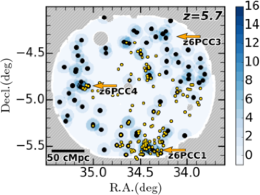
Figure 8.— Sky distribution of the $z=5.7$ LAEs (black filled circles) with the surface overdensity contours (black lines) in the $NB816$ UD-SXDS field. Higher density regions are shown with bluer colors. The yellow filled circles represent spectroscopically-confirmed LAEs. Extended Ly$\alpha$ sources found in Shibuya et al. (2017a) are marked with the black filled squares. The black lines correspond to the 5$\sigma$ to 8$\sigma$ significance levels of overdensity $\delta$ with a step of 1$\sigma$. Masked regions are presented with gray regions.

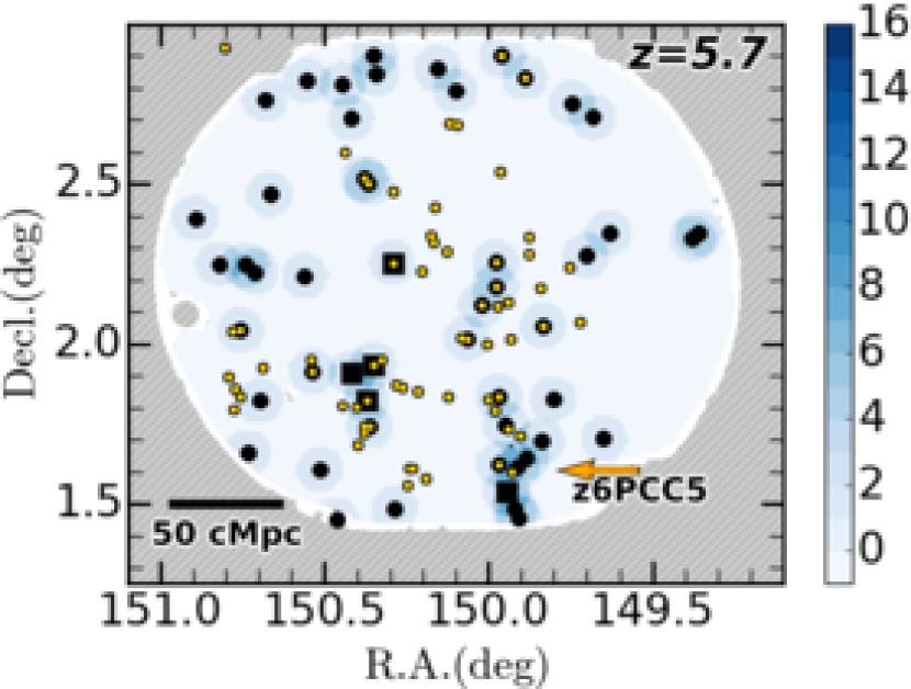
Figure 9.— Same as Figure 8, but for the $z=5.7$ LAEs in UD-COSMOS field.

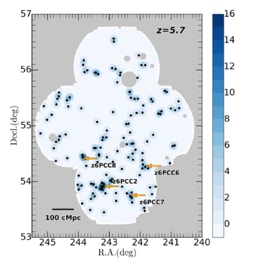
Figure 10.— Same as Figure 8, but for the $z=5.7$ LAEs in D-ELAIS-N1 field.

5. Results and Discussion

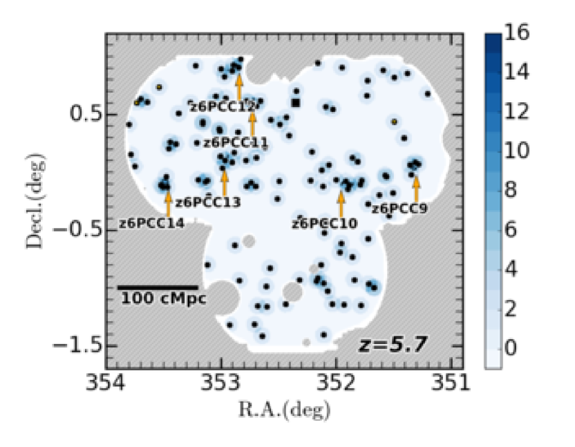
Figure 11.— Same as Figure 8, but for the $z=5.7$ LAEs in D-DEEP2-3 field.

5.1. Spatial Distribution of LAEs

5.1.1 Overdensity Measurements

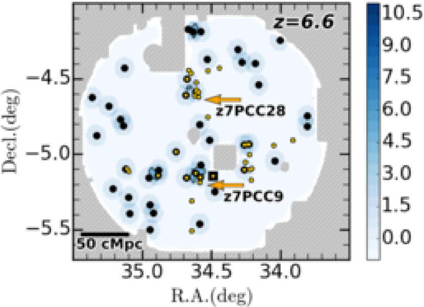
Figure 12.— Same as Figure 8, but for the $z=6.6$ LAEs in UD-SXDS field. The solid lines correspond to contours of $\delta$ from $3\sigma$ to $7\sigma$ significance levels with a step of 1$\sigma$.

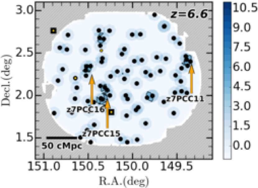
Figure 13.— Same as Figure 8, but for the $z=6.6$ LAEs in UD-COSMOS field.

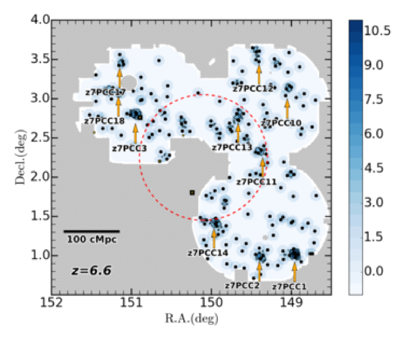
Figure 14.— Same as Figure 8, but for the $z=6.6$ LAEs in D-COSMOS field. The red-dashed line represents the region of the $z=6.6$ LAE UD-COSMOS field that is shown in Figure 13.

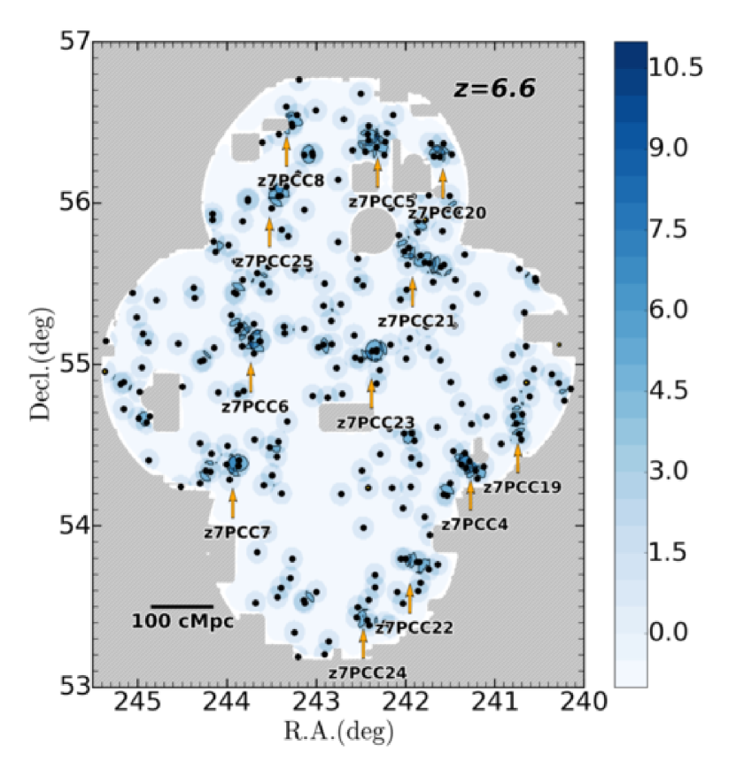
Figure 15.— Same as Figure 8, but for the $z=6.6$ LAEs in D-ELAIS-N1 field.

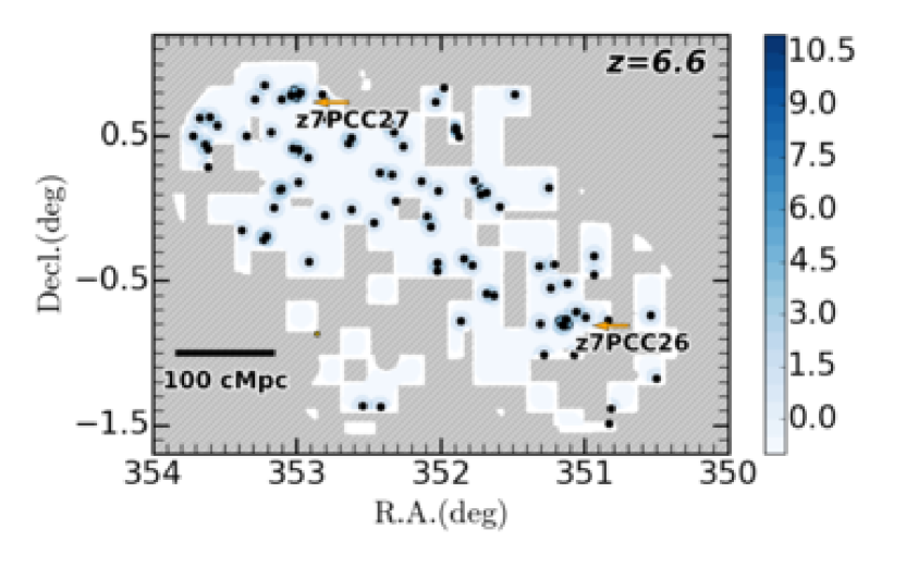
Figure 16.— Same as Figure 8, but for the $z=6.6$ LAEs in D-DEEP2-3 field.

We calculate LAE overdensities in each field with the HSC LAE samples. The definition of the LAE overdensity for our observational data is the same as the one for the model shown in Equation 9. We use a cylinder with a radius of 0.07 $\rm deg$ corresponding to 10 cMpc at $z\sim 6$. The height of the cylinder along a line of sight is 40 cMpc same as the width of the redshift distribution of the HSC LAEs.

Because some regions of the HSC narrowband data are not deep enough to calculate $\delta$ due to the data quality, we should not use the HSC LAEs found in the shallow regions for the density evaluation. The HSC imaging data are divided into $1.7\times 1.7\>\rm deg^{2}$ rectangular tracts that are made of $0.2\times 0.2\>\rm deg^{2}$ rectangular patches. We estimate a $5\sigma$ limiting magnitude of each patch in the $NB816$ ($NB921$) data for $z=5.7$ (6.6) LAEs. We evaluate $\delta$ only in an area where the $5\sigma$ limiting magnitude of the $NB816$ ($NB921$) band is brighter than 24.5 (25.0) mag. These magnitude limits are determined to keep a high-detection completeness of LAEs (Konno et al. 2017). We assume that the number density of LAEs in the masked regions is the same as the mean number density of LAEs in all fields. We also do not evaluate $\delta$ for a cylinder, in which more than $50\%$ of the area is masked. We show the HSC LAE sky distribution and the overdensity maps at $z=5.7$ and $6.6$ in Figures 8-16. The solid lines correspond to contours of $\delta$ from 5 (3) $\sigma$ to 8 (7) $\sigma$ significance levels with a step of $1\sigma$ at $z=5.7$ ($6.6$). Note that the peak of the overdensity is not always centered at the highest density region. This is because the position of the peak has an uncertainty on a scale of 0.07 deg.

5.1.2 Overdensity Identifications

We find that $\delta$ values of the HSC LAEs in some regions significantly exceed beyond those expected by random distribution. These $\delta$ values are not explained by a random distribution of galaxies, but physical structures. We define a region with $\delta$ exceeding the $5\sigma$ level of the Poisson distribution as a high-density region (HDR). At $z=5.7$ $(6.6)$, $\delta=9.7$ $(6.6)$ corresponds to the $\simeq 5\sigma$ significance level. We find 14 (27) HDRs at $z=5.7$ ($6.6$) with $\delta>9.7$ $(6.6)$. There is an overdensity of $z=6.6$ LAEs at R.A.$=34.64$ deg and decl. $=-4.56$ whose $\delta$ is 6.1 slightly below the $\simeq 5\sigma$ significance level. This overdensity is reported by Chanchaiworawit et al. (2017). Although this does not meet the criterion of $\delta>6.6$, we include this overdensity to the sample of our HDRs. We thus obtain 14 (28) HDRs at $z=5.7$ ($6.6$).

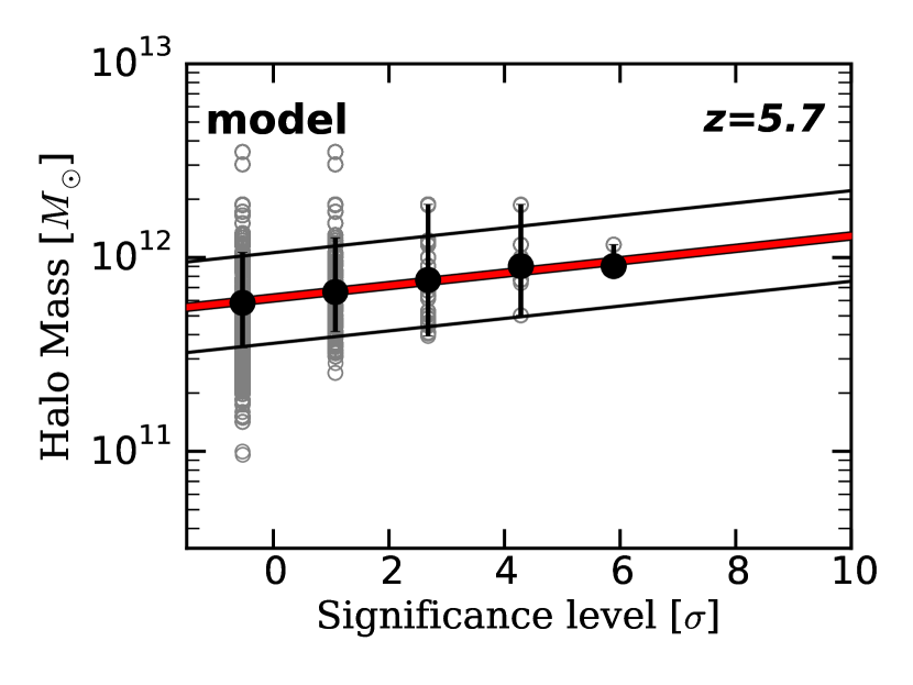
Figure 17.— Halo mass as a function of overdensity $\delta$ significance level for the model LAEs at $z=5.7$ (gray open circles) produced in the model of Inoue et al. (2018). The black filled circles with the error bars indicate the median values of the model LAEs. The red and black lines represent the best-fit linear function and the 68 $\%$ distribution of the model LAEs.

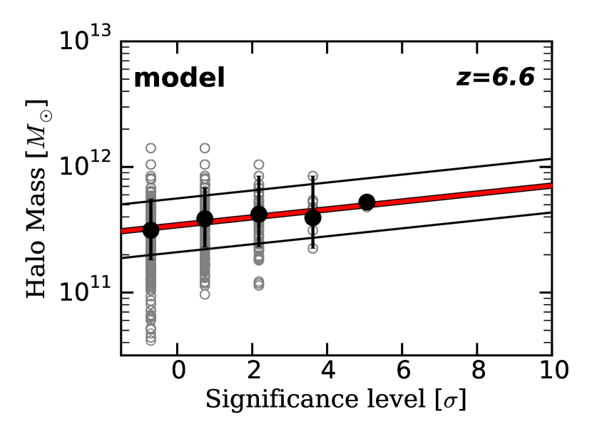
Figure 18.— Same as Figure 17, but for the $z=6.6$ model LAEs.

5.1.3 Halo Mass Estimates

From the theoretical model of Inoue et al. (2018), we obtain the halo mass $M_{\rm h}$ as a function of overdensity $\delta$. Because the halo mass is strongly related with the structure formation tightly connected with the abundance of halos and galaxies, we use LAEs in the model of Inoue et al. (2018) whose abundance is the same as those of the HSC LAEs. We define $M_{\rm h}$ as the most massive halo found in a cylinder volume used for the $\delta$ calculation. Figure 17 (18) shows $M_{\rm h}$ as a function of $\delta$ significance level at $z=5.7\>(6.6)$. We fit the $M_{\rm h}$ - $\delta$ relation with a linear function, and obtain $\log_{10}[M_{\rm h}/M_{\odot}]=0.032\delta+11.79$ $(\log_{10}[M_{\rm h}/M_{\odot}]=0.032\delta+11.54)$ at $z=5.7$ $(6.6)$.

We use the extended Press-Schechter model of Hamana et al. (2006) to estimate the present-day halo masses of the high-$z$ ($z=5.7$ and $6.6$) halos. Based on the $M_{\rm h}$ - $\delta$ relation, we find that  60 (58)% of the $z=5.7$ ($6.6$) $M_{\rm h}$-halos in the HDRs are expected to evolve into present-day cluster haloes with a mass of $>10^{14}\>\rm M_{\odot}$ by $z=0$. Because more than a half of the $M_{\rm h}$-halos in the HDRs are progenitors of the present-day clusters, we regard the 14 (28) HDRs at $z=5.7$ ($6.6$) as protocluster candidates. The 14 (28) protocluster candidates are listed in Table 6. Here we name the $z=5.7$ (6.6) protocluster candidates as HSC-z6 (7) PCC.

We compare the abundance of the protocluster candidates with that of present-day clusters. The comoving survey volumes of the HSC observations are $\sim 1.2\times 10^{7}\>\rm Mpc^{3}$ and $\sim 1.9\times 10^{7}\>\rm Mpc^{3}$ at $z=5.7$ and 6.6, respectively. Because there exists one present-day cluster with a mass of $1-3\times 10^{14}M_{\odot}$ in a volume of $\sim 5\times 10^{5}$ Mpc³ (Reiprich & Böhringer 2002), it is expected that our survey volumes at $z=5.7$ and $6.6$ include $\sim 20$ and $\sim 40$ present-day clusters, respectively. These numbers are comparable with those of our protocluster candidates, 14 and 28.

5.1.4 Three-Dimensional Distribution and Protocluster Candidates

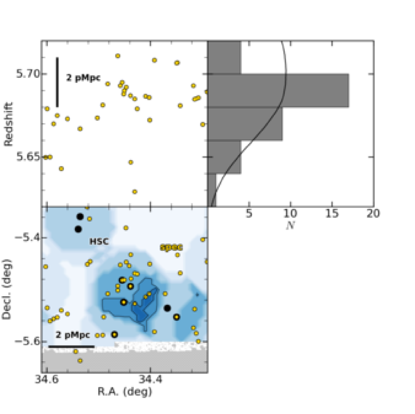
Figure 19.— Three-dimensional map of HSC-z6PCC1. The bottom panel presents the distribution of the LAEs projected on the sky. The top-left panel shows the distribution of the LAEs on the plane of transverse (east to west) vs. radial (redshift) directions. The black filled circles represent the HSC LAEs with $NB816<24.5$ used for the overdensity evaluation, while the yellow filled circles denote the spectroscopically-confirmed LAEs that include faint sources with $NB816\simeq 25-26$. The black solid lines in the bottom panel indicate the contours of the overdensity significance levels from 5$\sigma$ to 8$\sigma$ with a step of 1$\sigma$. The masked regions are shown with the gray regions. The top right panel shows the redshift distribution of the spectroscopically-confirmed LAEs. The black line indicates the mean expected number of LAEs in the region.

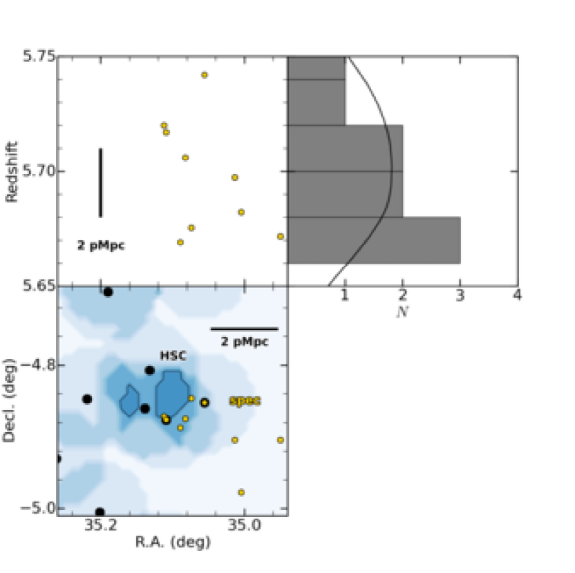
Figure 20.— Same as Figure 19, but for HSC-z6PCC4.

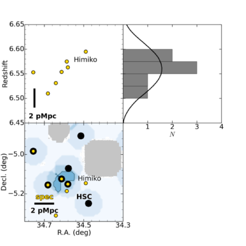
Figure 21.— Same as Figure 19, but for HSC-z7PCC9. The black filled circles represent the HSC LAEs with $NB921<25.0$. The yellow circles indicate the spectroscopically-confirmed LAEs including sources with $NB921\simeq 25-26$.

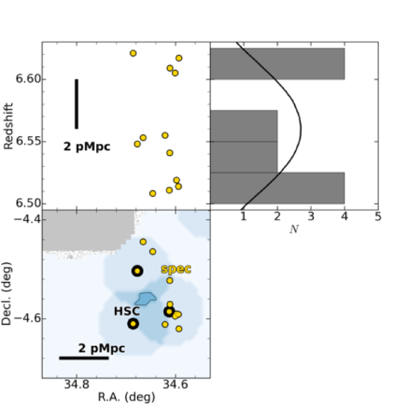
Figure 22.— Same as Figure 21, but for HSC-z7PCC28.

Based on the follow-up spectroscopic observations in Section 3, we find 3 (3) protocluster candidates at $z=5.7\>(6.6)$ which have (a) spectroscopically confirmed LAE(s). These are HSC-z6PCC1, HSC-z6PCC4, and HSC-z6PCC5 (HSC-z7PCC3, HSC-z7PCC9, and HSC-z7PCC28) at $z=5.7$ ($6.6$). The three-dimensional distributions of HSC-z6PCC1, HSC-z6PCC4, HSC-z7PCC9, and HSC-z7PCC28 are shown in Figures 19, 20, 21, 22, respectively. Here we explain three examples of the protocluster candidates, HSC-z6PCC1, HSC-z7PCC9, and HSC-z7PCC28.

HSC-z6PCC1

HSC-z6PCC1 (Figure 19) consists of $z=5.7$ LAEs in the southern part of UD SXDS. Twelve spectroscopically confirmed LAEs exist within a distance of $\sim 1$ physical Mpc (pMpc). The redshift averaged over the spectroscopically-confirmed LAEs is $z=5.692$. HSC-z6PCC1 is the same structure as Clump A that is a protocluster identified by Ouchi et al. (2005). Six out of the 12 spectroscopically confirmed LAEs are included in Clump A.

HSC-z7PCC9

HSC-z7PCC9 at $z=6.6$ (Figure 21) is located at the center of UD SXDS. HSC-z7PCC9 consists of five spectroscopically confirmed LAEs, including the giant Ly$\alpha$ nebula ’Himiko’ (Ouchi et al. 2009). The average redshift of the LAEs is $z=6.574$. If all of the LAEs of HSC-z7PCC9 are spectroscopically confirmed, HSC-z7PCC9 could be one of the earliest protoclusters found to date.

HSC-z7PCC28

HSC-z7PCC28 (Figure 22) is placed at the northern part of UD SXDS at $z=6.6$. This is the protocluster candidate reported by Chanchaiworawit et al. (2017), although the overdensity of HSC-z7PCC28 is $\delta=6.1$ slightly below the $5\sigma$ significance level (Section 5.1.2). There are five spectroscopically confirmed LAEs in a sphere with a radius of $\sim 1$ pMpc. The redshift averaged over the spectroscopically-confirmed LAEs is $z=6.534$. Three out of the five spectroscopically confirmed LAEs are included in the members of the overdensity shown in Chanchaiworawit et al. (2017).

5.2. Implications for Cosmic Reionization

5.2.1 Spatial Correlation between Bright LAEs and Overdensities

To study the origin of the bright-end excess of Ly$\alpha$ luminosity functions at $z=5.7$ and $6.6$ (Konno et al. 2017), we investigate the correlation between Ly$\alpha$ luminosity and overdensity. Figure 23 (24) shows the relation between Ly$\alpha$ luminosity $L_{\rm Ly\alpha}$ and large-scale LAE overdensity $\delta_{\rm LS}$ for $z=5.7$ ($6.6$) LAEs. Here $\delta_{\rm LS}$ is defined with a circle with a radius of 0.20 $\rm deg$ that corresponds to $\sim 30$ cMpc at $z\sim 6$ comparable with the size of typical ionized bubbles at this redshift predicted by Furlanetto et al. (2006) (cf. $\delta$ defined with a circular radius of 0.07 deg; see Section 5.1). With the results of Figures 23 and 24, we calculate a Spearman’s rank correlation coefficient $\rho$ and a p-value to test the existence of the correlation between $L_{\rm Ly\alpha}$ and $\delta_{\rm LS}$. We obtain $\rho=-0.017$ $(0.020)$ with p-value$=0.75$ $(0.68)$ for $z=5.7$ ($6.6$) LAEs, which suggest that there are no significant correlations between $L_{\rm Ly\alpha}$ and $\delta_{\rm LS}$. This result indicates that bright $L_{\rm Ly\alpha}$ LAEs are not selectively placed at the overdensity and that there is no clear evidence connecting the bright-end LF excess and the ionized bubble. Because the statistical uncertainty of this analysis is still large, it is not a conclusive result. However, there is an increasing possibility that the ionized bubbles and the bright-end LF excess may not be related. For the other possible origins of the bright-end excess, Konno et al. (2017) discuss the AGN/low-$z$ contamination and the blended merging galaxies. We should discuss these other possibilities more seriously.

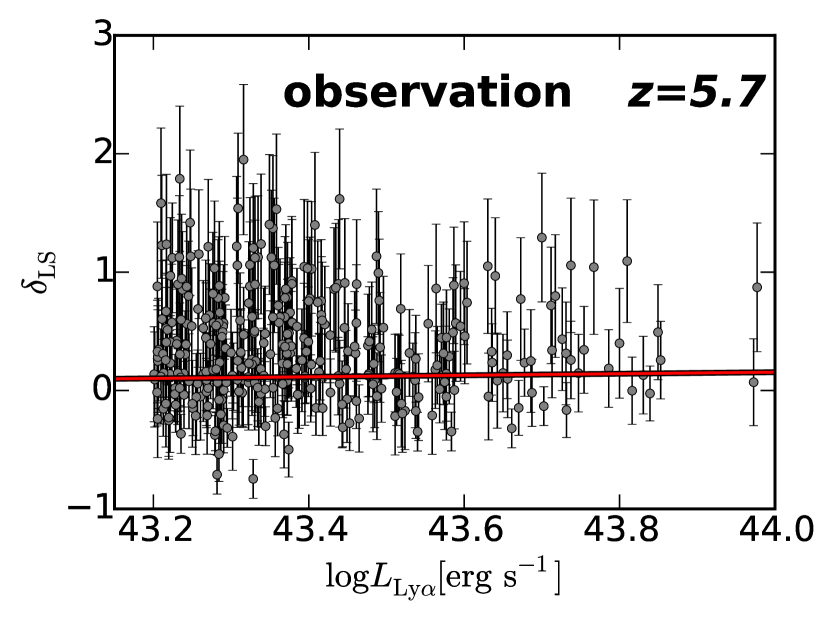
Figure 23.— Ly$\alpha$ luminosity $L_{\rm Ly\alpha}$ as a function of large-scale overdensity $\delta_{\rm LS}$ for the HSC LAEs at $z=5.7$ (gray circles). The red line indicates the best-fit linear function.

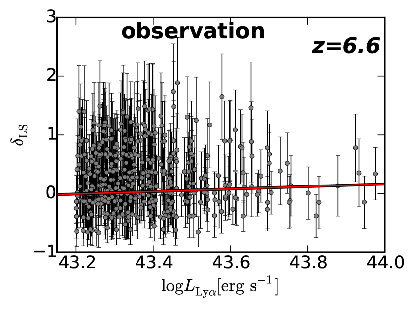
Figure 24.— Same as Figure 23, but for the HSC LAEs at $z=6.6$.

5.2.2 Correlation between Ly$\alpha\$ EW and Overdensity

Figure 25 (26) presents $EW^{\rm rest}_{\rm Ly\alpha}$ as a function of $\delta$ at $z=5.7$ $(6.6)$. $EW^{\rm rest}_{\rm Ly\alpha}$ is estimated in the same manner as Shibuya et al. (2017a). We calculate $EW^{\rm rest}_{\rm Ly\alpha}$ of LAEs from the $NB816$ ($NB921$) and $z$ ($y$) band magnitudes. We use the subsamples of the LAEs in a range of $\delta$, and obtain a median value of $EW^{\rm rest}_{\rm Ly\alpha}$ at a given $\delta$. We perform chi-square fitting of the linear function to the $EW^{\rm rest}_{\rm Ly\alpha}$ - $\delta$ relations, and obtain the best-fit parameters, $\alpha$ and $EW_{\delta=0}$, defined in Section 4. Because the theoretical model predicts that the value of $\alpha$ increases from $z=5.7$ to $6.6$ (Section 4), we show redshift evolution of $\alpha$ of the observational results in Figure 27. Figure 27 indicates that there is no significant evolution of the $EW^{\rm rest}_{\rm Ly\alpha}$ - $\delta$ relation from $z=5.7$ to $6.6$ beyond the uncertainties accomplished with our HSC data so far obtained.

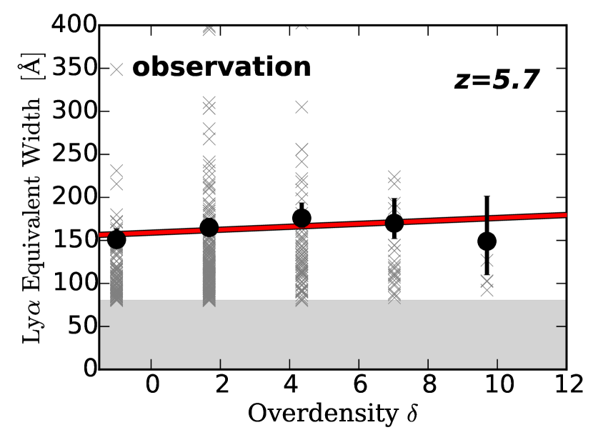
Figure 25.— Ly$\alpha$ EW and overdensity $\delta$ for the HSC LAEs at $z=5.7$ (gray crosses). The black circles with the error bars indicate the median values of the HSC LAEs at a given $\delta$. The red line represents the best-fit linear function. The gray region indicates the Ly$\alpha$ EW selection limit.

Figure 26.— Same as Figure 25, but for the HSC LAEs at $z=6.6$.

5.2.3 Comparison with the Theoretical Model

We compare the results of Section 5.2.2 with the theoretical model of Inoue et al. (2018). We select mock LAEs which are brighter than 25.0 mag in narrowbands, which is the same magnitude limit as the HSC LAE $\delta$ estimates. We also apply the selection limits of the Ly$\alpha$ EW which are similar to those of the HSC LAE samples. We thus obtain 447 (80) mock LAEs for $z=5.7$ (6.6) that are referred to as ’HSC mock’. We derive the best-fit parameters and errors for HSC mock in the same way as Section 5.2.2. Note that we define the error of $EW^{\rm rest}_{\rm Ly\alpha}$ as the range of 68$\%$ distribution. Figure 27 presents redshift evolution of the slope $\alpha$ of ’HSC mock’ at $z=5.7$ and $6.6$. (In this model, the average neutral hydrogen fraction in the IGM at $z=5.7$ and $6.6$ are $\log{x_{\rm HI}}=-3.9$ and $-0.36$, respectively.) The model does not show the significant evolution of the $EW^{\rm rest}_{\rm Ly\alpha}$ - $\delta$ relation beyond the statistical errors, which is consistent with those of the HSC LAE samples. The model suggests that the present HSC LAE samples are not large enough to test the existence of the ionized bubbles and the inside-out scenario of cosmic reionization. The HSC survey is underway, which will significantly enlarge the sample with the wider and deeper data for LAEs at $z=5.7$ and $6.6$ and make a new sample of LAEs at $z=7.3$. There is a possibility that the evolution of the $EW^{\rm rest}_{\rm Ly\alpha}$ - $\delta$ relation from $z=5.7$ to $7.3$ may be identified by the upcoming HSC observations providing the large samples of LAEs at $z=5.7-7.3$. The ionized bubbles and the inside-out scenario should be tested in the forthcoming studies with the large samples of LAEs at $z=5.7-7.3$.

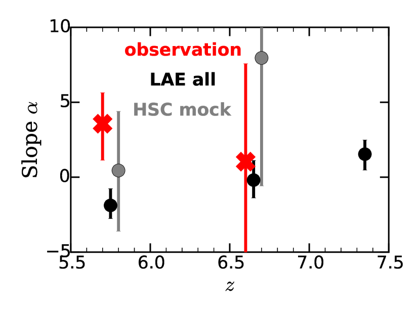
Figure 27.— Redshift evolution of the slope $\alpha$. The red crosses denote the HSC LAEs, while the gray (black) circles show the model predictions with the samples of ’HSC mock’ and LAE all’, respectively. To avoid overlaps of the symbols, we slightly shift black and grey circles by 0.05 and 0.10 in redshift, respectively.

6. Summary

In this study, we study LAE overdensities at $z=5.7$ and $6.6$ with the early datasets of the HSC SSP survey based on the 2,230 LAEs obtained in the SILVERRUSH program. We identify the LAE overdensities and discuss cosmic reionization with the properties of LAEs, overdensity $\delta$, Ly$\alpha$ luminosity $L_{\rm Ly\alpha}$, and the rest-frame Ly$\alpha$ equivalent width $EW^{\rm rest}_{\rm Ly\alpha}$. Our major results are listed below:

1. We calculate the LAE overdensity $\delta$ with the samples of the HSC LAEs at $z=5.7$ and $6.6$. We identify 14 (28) $z=5.7$ $(6.6)$ LAE overdensities with the $\gtrsim 5\sigma$ significance level, six out of which have $1-12$ spectroscopically confirmed LAEs. We compare the LAE overdensities with the the cosmological Ly $\alpha$ radiative transfer models, and find that more than a half of these LAE overdensities (60% and 58% of the LAE overdensities at $z=5.7$ and $6.6$) are progenitors of the present-day clusters with a mass of $\gtrsim 10^{14}M_{\odot}$. These 14 (28) LAE overdensities are thus protocluster candidates at $z=5.7$ $(6.6)$ that are listed in Table 6.

2. We investigate the correlation between $L_{\rm Ly\alpha}$ and $\delta$ with the HSC LAEs. We obtain a Spearman’s rank correlation coefficient $\rho=-0.017$ $(0.020)$ with p-value=0.75 $(0.68)$ for $z=5.7$ ($6.6$) LAEs, which indicate that there is no evidence of significant correlations between $L_{\rm Ly\alpha}$ and $\delta$ beyond the observational uncertainties. Our result is related to the recent discussion about the bright-end excess of Ly$\alpha$ LFs at $z=5.7$ and $6.6$ such found in Konno et al. (2017). For the physical reason of the bright-end excess, there is an idea that bright galaxies selectively existing in an overdensity region are placed near the center of the ionized bubbles that allow Ly$\alpha$ photons escape from the partly neutral IGM at the EoR. Because our results show no correlation between $L_{\rm Ly\alpha}$ and $\delta$, there is no evidence supporting this idea.

3. We study the relations between $EW^{\rm rest}_{\rm Ly\alpha}$ and $\delta$ at $z=5.7$ and $6.6$. We fit a linear function to the $EW^{\rm rest}_{\rm Ly\alpha}$-$\delta$ data, and find that the slope (the relation) does not evolve (is not steepened) from $z=5.7$ to $6.6$ beyond the errors. The cosmological reionization model with the Ly$\alpha$ radiative transfer suggests that the slope is steepened towards the early EoR with a high neutral hydrogen fraction in the inside-out reionization scenario, because the ionized bubbles around galaxy overdensities ease the escape of Ly$\alpha$ emission from the partly neutral IGM at the EoR. Although the model suggests that the statistical accuracy of our HSC data is not high enough to investigate this steepening, so far we find no such steepening in the available HSC data. There is a possibility of detecting the evolution of the $EW^{\rm rest}_{\rm Ly\alpha}$ - $\delta$ relation from $z=5.7$ to $7.3$ by the scheduled HSC narrowband observations that will make larger samples of LAEs at $z=5.7-6.6$ as well as a new sample of LAEs at $z=7.3$.

Table 4Spectroscopic Sample of the $z=5.7$ LAEs

ID	R.A. (J2000)	Decl. (J2000)	$z$	Reference
(1)	(2)	(3)	(4)	(5)
UD SXDS
HSC J021714-050844	$34.3104$	$-5.1456$	$5.685$	This Study
HSC J021712-050748	$34.3027$	$-5.1302$	$5.699$	This Study
HSC J021728-051217	$34.3678$	$-5.2047$	$5.676$	This Study
HSC J021750-050203	$34.4619$	$-5.0342$	$5.708$	This Study
…	…	…	…	…

Note. — Spectroscopically identified LAEs at $z=5.7$. See the full sample catalog in the version published in ApJ. (1) Object ID; (2) right ascension; (3) declination; (4) spectroscopic redshift; (5) reference of the spectroscopic redshift. O05 = Ouchi et al. (2005), O08 = Ouchi et al. (2008), M12 = Mallery et al. (2012), and SH17 = Shibuya et al. (2017b).

Table 5Spectroscopic Sample of the $z=6.6$ LAEs

ID	R.A. (J2000)	Decl. (J2000)	$z$	Reference
(1)	(2)	(3)	(4)	(5)
UD SXDS
HSC J021703-045619	$34.2644$	$-4.9386$	$6.589$	O10
HSC J021820-051109	$34.5862$	$-5.1861$	$6.575$	O10
HSC J021819-050900	$34.5808$	$-5.1502$	$6.563$	O10
HSC J021757-050844	$34.4899$	$-5.1457$	$6.595$	O10
…	…	…	…	…

Note. — Spectroscopically identified LAEs at $z=6.6$. See the full sample catalog in the version published in ApJ. (1) Object ID; (2) right ascension; (3) declination; (4) spectroscopic redshift; (5) reference of the spectroscopic redshift. O10 = Ouchi et al. (2010), SO15 = Sobral et al. (2015), HU16 = Hu et al. (2016), SH17 = Shibuya et al. (2017b), and C$\&$G17 = Chanchaiworawit et al. (2017) and Guzmán et al. (in preparation).

Table 6Protocluster Candidates

Name	Layer	Field	R.A. (J2000)	Decl. (J2000)	overdensity $\delta$	significance	$n_{\rm photo}$	$n_{\rm spec}$	$z_{\rm spec}$
(1)	(2)	(3)	(4)	(5)	(6)	(7)	(8)	(9)	(10)
$z=5.7$
HSC-z6PCC3	UD	SXDS	34.26	$-4.32$	9.7	5.4	4 (5)	0	-
HSC-z6PCC1	UD	SXDS	34.42	$-5.54$	15.0	8.4	6 (7)	12	5.692
HSC-z6PCC4	UD	SXDS	35.16	$-4.85$	9.7	5.4	4 (7)	4	5.719
HSC-z6PCC5	UD	COSMOS	149.94	1.60	9.7	5.4	4 (5)	2	5.686
HSC-z6PCC6	Deep	ELAIS-N1	241.84	54.27	9.7	5.4	4 (4)	0	-
HSC-z6PCC7	Deep	ELAIS-N1	242.32	53.77	9.7	5.4	4 (5)	0	-
HSC-z6PCC2	Deep	ELAIS-N1	243.22	53.92	15.0	8.4	6 (8)	0	-
HSC-z6PCC8	Deep	ELAIS-N1	243.89	54.42	9.7	5.4	4 (4)	0	-
HSC-z6PCC9	Deep	DEEP2-3	351.30	0.03	9.7	5.4	4 (4)	0	-
HSC-z6PCC10	Deep	DEEP2-3	351.95	$-0.10$	9.7	5.4	4 (6)	0	-
HSC-z6PCC11	Deep	DEEP2-3	352.72	0.60	9.7	5.4	4 (4)	0	-
HSC-z6PCC12	Deep	DEEP2-3	352.84	0.91	9.7	5.4	4 (6)	0	-
HSC-z6PCC13	Deep	DEEP2-3	352.97	0.08	9.7	5.4	4 (4)	0	-
HSC-z6PCC14	Deep	DEEP2-3	353.45	$-0.10$	9.7	5.4	4 (4)	0	-
$z=6.6$
HSC-z7PCC9	UD	SXDS	34.62	$-5.13$	6.6	4.6	4 (4)	3	6.574
HSC-z7PCC28	UD	SXDS	34.64	$-4.56$	6.1	3.8	3 (3)	5	6.537
HSC-z7PCC11	UD	COSMOS	149.35	2.41	6.6	4.6	4 (4)	0	-
HSC-z7PCC15	UD	COSMOS	150.30	2.00	6.6	4.6	4 (6)	0	-
HSC-z7PCC16	UD	COSMOS	150.48	2.29	6.6	4.6	4 (8)	0	-
HSC-z7PCC1	Deep	COSMOS	148.96	1.02	10.5	7.2	6 (6)	0	-
HSC-z7PCC10	Deep	COSMOS	149.05	3.10	6.6	4.6	4 (4)	0	-
HSC-z7PCC2	Deep	COSMOS	149.40	1.03	8.5	5.9	5 (5)	0	-
HSC-z7PCC12	Deep	COSMOS	149.41	3.54	6.6	4.6	4 (4)	0	-
HSC-z7PCC13	Deep	COSMOS	149.67	2.79	6.6	4.6	4 (4)	0	-
HSC-z7PCC14	Deep	COSMOS	149.97	1.45	6.6	4.6	4 (6)	0	-
HSC-z7PCC3	Deep	COSMOS	150.95	2.78	8.5	5.9	5 (5)	1	6.575
HSC-z7PCC17	Deep	COSMOS	151.15	3.49	6.6	4.6	4 (4)	0	-
HSC-z7PCC18	Deep	COSMOS	151.16	3.13	6.6	4.6	4 (2)	0	-
HSC-z7PCC19	Deep	ELAIS-N1	240.74	54.63	6.6	4.6	4 (4)	0	-
HSC-z7PCC4	Deep	ELAIS-N1	241.27	54.4	8.6	5.9	5 (5)	0	-
HSC-z7PCC20	Deep	ELAIS-N1	241.58	56.33	6.6	4.6	4 (4)	0	-
HSC-z7PCC21	Deep	ELAIS-N1	241.92	55.66	6.6	4.6	4 (7)	0	-
HSC-z7PCC22	Deep	ELAIS-N1	241.95	53.76	6.6	4.6	4 (4)	0	-
HSC-z7PCC5	Deep	ELAIS-N1	242.31	56.4	8.6	5.9	5 (5)	0	-
HSC-z7PCC23	Deep	ELAIS-N1	242.38	55.03	6.6	4.6	4 (4)	0	-
HSC-z7PCC24	Deep	ELAIS-N1	242.47	53.48	6.6	4.6	4 (4)	0	-
HSC-z7PCC8	Deep	ELAIS-N1	243.33	56.53	6.7	4.6	4 (4)	0	-
HSC-z7PCC25	Deep	ELAIS-N1	243.52	56.03	6.6	4.6	4 (5)	0	-
HSC-z7PCC6	Deep	ELAIS-N1	243.73	55.13	8.6	5.9	5 (5)	0	-
HSC-z7PCC7	Deep	ELAIS-N1	243.93	54.35	8.6	5.9	5 (5)	0	-
HSC-z7PCC26	Deep	DEEP2-3	351.09	$-0.77$	6.6	4.6	4 (4)	0	-
HSC-z7PCC27	Deep	DEEP2-3	353.04	0.77	6.6	4.6	4 (4)	0	-

Note. — (1) object ID; (2) layer; (3) field; (4) right ascension of the center of the member LAEs (deg); (5) declination of the center of the member LAEs (deg); (6)-(7) highest $\delta$ and the significance level in the protocluster candidates; (8) number of the HSC LAEs in a 0.07 deg radius from the center of the protocluster candidates; (9) number of the spectroscopically-confirmed LAEs in 10 cMpc from the center of the protocluster candidates; (10) average redshift value of the spectroscopically-confirmed LAEs.

References

- Aihara et al. (2017) Aihara, H., et al. 2017, ArXiv e-prints, arXiv: 1704.05858
- Axelrod et al. (2010) Axelrod, T., Kantor, J., Lupton, R. H., & Pierfederici, F. 2010, in Proc. SPIE, Vol. 7740, Software and Cyberinfrastructure for Astronomy, 774015
- Bertin & Arnouts (1996) Bertin, E., & Arnouts, S. 1996, A&AS, 117, 393
- Bolton et al. (2011) Bolton, J. S., Haehnelt, M. G., Warren, S. J., Hewett, P. C., Mortlock, D. J., Venemans, B. P., McMahon, R. G., & Simpson, C. 2011, MNRAS, 416, L70
- Bosch et al. (2017) Bosch, J., et al. 2017, ArXiv e-prints, arXiv:1705.06766
- Bouwens et al. (2015) Bouwens, R. J., Illingworth, G. D., Oesch, P. A., Caruana, J., Holwerda, B., Smit, R., & Wilkins, S. 2015, ApJ, 811, 140
- Chanchaiworawit et al. (2017) Chanchaiworawit, K., et al. 2017, MNRAS, 469, 2646
- Chiang et al. (2013) Chiang, Y.-K., Overzier, R., & Gebhardt, K. 2013, ApJ, 779, 127
- Chiang et al. (2017) Chiang, Y.-K., Overzier, R. A., Gebhardt, K., & Henriques, B. 2017, ApJ, 844, L23
- Chornock et al. (2013) Chornock, R., Berger, E., Fox, D. B., Lunnan, R., Drout, M. R., Fong, W.-f., Laskar, T., & Roth, K. C. 2013, ApJ, 774, 26
- Davis et al. (2003) Davis, M., et al. 2003, in Proc. SPIE, Vol. 4834, Discoveries and Research Prospects from 6- to 10-Meter-Class Telescopes II, ed. P. Guhathakurta, 161
- Dijkstra et al. (2016) Dijkstra, M., Gronke, M., & Venkatesan, A. 2016, ApJ, 828, 71
- Dijkstra et al. (2011) Dijkstra, M., Mesinger, A., & Wyithe, J. S. B. 2011, MNRAS, 414, 2139
- Dressler et al. (2006) Dressler, A., Hare, T., Bigelow, B. C., & Osip, D. J. 2006, in Proc. SPIE, Vol. 6269, Society of Photo-Optical Instrumentation Engineers (SPIE) Conference Series, 62690F
- Faber et al. (2003) Faber, S. M., et al. 2003, in Proc. SPIE, Vol. 4841, Instrument Design and Performance for Optical/Infrared Ground-based Telescopes, ed. M. Iye & A. F. M. Moorwood, 1657
- Fan et al. (2006) Fan, X., et al. 2006, AJ, 132, 117
- Franck & McGaugh (2016a) Franck, J. R., & McGaugh, S. S. 2016a, ApJ, 833, 15
- Franck & McGaugh (2016b) Franck, J. R., & McGaugh, S. S. 2016b, ApJ, 817, 158
- Furlanetto et al. (2006) Furlanetto, S. R., Zaldarriaga, M., & Hernquist, L. 2006, MNRAS, 365, 1012
- Furusawa et al. (2017) Furusawa, H., et al. 2017, Publications of the Astronomical Society of Japan, psx079
- Goto et al. (2011) Goto, T., Utsumi, Y., Hattori, T., Miyazaki, S., & Yamauchi, C. 2011, MNRAS, 415, L1
- Guzmán et al. (in preparation) Guzmán, R., et al. in preparation, in Early stages of Galaxy Cluster Formation, 12
- Hamana et al. (2006) Hamana, T., Yamada, T., Ouchi, M., Iwata, I., & Kodama, T. 2006, MNRAS, 369, 1929
- Harikane et al. (2017a) Harikane, Y., et al. 2017a, ArXiv e-prints, arXiv:1704.06535
- Harikane et al. (2017b) Harikane, Y., et al. 2017b, ArXiv e-prints, arXiv:1711.03735
- Hasegawa et al. (in preparation) Hasegawa, K., et al. 2017, in prep
- Hu et al. (2016) Hu, E. M., Cowie, L. L., Songaila, A., Barger, A. J., Rosenwasser, B., & Wold, I. G. B. 2016, ApJ, 825, L7
- Iliev et al. (2006) Iliev, I. T., Mellema, G., Pen, U.-L., Merz, H., Shapiro, P. R., & Alvarez, M. A. 2006, MNRAS, 369, 1625
- Inoue et al. (2018) Inoue, A. K., et al. 2018, submitted to PASJ
- Ishigaki et al. (2016) Ishigaki, M., Ouchi, M., & Harikane, Y. 2016, ApJ, 822, 5
- Ishigaki et al. (2017) Ishigaki, M., Kawamata, R., Ouchi, M., Oguri, M., & Shimasaku, K. 2017, ArXiv e-prints, arXiv:1702.04867
- Ivezic et al. (2008) Ivezic, Z., et al. 2008, ArXiv e-prints, arXiv: 0805.2366
- Iye et al. (2004) Iye, M., et al. 2004, PASJ, 56, 381
- Jensen et al. (2014) Jensen, H., Hayes, M., Iliev, I. T., Laursen, P., Mellema, G., & Zackrisson, E. 2014, MNRAS, 444, 2114
- Jurić et al. (2015) Jurić, M., et al. 2015, ArXiv e-prints, arXiv:1512.07914
- Kakiichi et al. (2016) Kakiichi, K., Dijkstra, M., Ciardi, B., & Graziani, L. 2016, MNRAS, 463, 4019
- Kashikawa et al. (2006) Kashikawa, N., et al. 2006, ApJ, 648, 7
- Kashikawa et al. (2011) Kashikawa, N., et al. 2011, ApJ, 734, 119
- Komiyama et al. (2017) Komiyama, Y., et al. 2017, Publications of the Astronomical Society of Japan, psx069
- Konno et al. (2014) Konno, A., et al. 2014, ApJ, 797, 16
- Konno et al. (2017) Konno, A., et al. 2017, ArXiv e-prints, arXiv:1705.01222
- Lee et al. (2012) Lee, J. C., et al. 2012, PASP, 124, 782
- Lovell et al. (2017) Lovell, C. C., Thomas, P. A., & Wilkins, S. M. 2017, ArXiv e-prints, arXiv:1710.02148
- Magnier et al. (2013) Magnier, E. A., et al. 2013, ApJS, 205, 20
- Malhotra & Rhoads (2004) Malhotra, S., & Rhoads, J. E. 2004, ApJ, 617, L5
- Mallery et al. (2012) Mallery, R. P., et al. 2012, ApJ, 760, 128
- Matthee et al. (2015) Matthee, J., Sobral, D., Santos, S., Röttgering, H., Darvish, B., & Mobasher, B. 2015, MNRAS, 451, 400
- McGreer et al. (2015) McGreer, I. D., Mesinger, A., & D’Odorico, V. 2015, MNRAS, 447, 499
- McQuinn (2012) McQuinn, M. 2012, MNRAS, 426, 1349
- Mesinger et al. (2013) Mesinger, A., Ferrara, A., & Spiegel, D. S. 2013, MNRAS, 431, 621
- Miralda-Escudé et al. (2000) Miralda-Escudé, J., Haehnelt, M., & Rees, M. J. 2000, ApJ, 530, 1
- Miyazaki et al. (2017) Miyazaki, S., et al. 2017, Publications of the Astronomical Society of Japan, psx063
- Miyazaki et al. (2002) Miyazaki, S., et al. 2002, PASJ, 54, 833
- Momcheva et al. (2013) Momcheva, I. G., Lee, J. C., Ly, C., Salim, S., Dale, D. A., Ouchi, M., Finn, R., & Ono, Y. 2013, AJ, 145, 47
- Nakamoto et al. (2001) Nakamoto, T., Umemura, M., & Susa, H. 2001, MNRAS, 321, 593
- Ono et al. (2012) Ono, Y., et al. 2012, ApJ, 744, 83
- Ono et al. (2017) Ono, Y., et al. 2017, ArXiv e-prints, arXiv:1704.06004
- Ota et al. (2010) Ota, K., et al. 2010, ApJ, 722, 803
- Ouchi et al. (2005) Ouchi, M., et al. 2005, ApJ, 620, L1
- Ouchi et al. (2008) Ouchi, M., et al. 2008, ApJS, 176, 301
- Ouchi et al. (2009) Ouchi, M., et al. 2009, ApJ, 696, 1164
- Ouchi et al. (2010) Ouchi, M., et al. 2010, ApJ, 723, 869
- Ouchi et al. (2017) Ouchi, M., et al. 2017, ArXiv e-prints, arXiv:1704.07455
- Overzier (2016) Overzier, R. A. 2016, A&A Rev., 24, 14
- Planck Collaboration et al. (2016) Planck Collaboration, et al. 2016, A&A, 594, A13
- Reiprich & Böhringer (2002) Reiprich, T. H., & Böhringer, H. 2002, ApJ, 567, 716
- Robertson et al. (2015) Robertson, B. E., Ellis, R. S., Furlanetto, S. R., & Dunlop, J. S. 2015, ApJ, 802, L19
- Santos et al. (2016) Santos, S., Sobral, D., & Matthee, J. 2016, MNRAS, 463, 1678
- Schlafly et al. (2012) Schlafly, E. F., et al. 2012, ApJ, 756, 158
- Shibuya et al. (2017a) Shibuya, T., et al. 2017a, ArXiv e-prints, arXiv:1704.08140
- Shibuya et al. (2017b) Shibuya, T., et al. 2017b, ArXiv e-prints, arXiv: 1705.00733
- Sobral et al. (2015) Sobral, D., Matthee, J., Darvish, B., Schaerer, D., Mobasher, B., Röttgering, H. J. A., Santos, S., & Hemmati, S. 2015, ApJ, 808, 139
- Stark et al. (2011) Stark, D. P., Ellis, R. S., & Ouchi, M. 2011, ApJ, 728, L2
- Tonry et al. (2012) Tonry, J. L., et al. 2012, ApJ, 750, 99
- Toshikawa et al. (2012) Toshikawa, J., et al. 2012, ApJ, 750, 137
- Toshikawa et al. (2014) Toshikawa, J., et al. 2014, ApJ, 792, 15
- Toshikawa et al. (2017) Toshikawa, J., et al. 2017, ArXiv e-prints, arXiv:1708.09421
- Utsumi et al. (2010) Utsumi, Y., Goto, T., Kashikawa, N., Miyazaki, S., Komiyama, Y., Furusawa, H., & Overzier, R. 2010, ApJ, 721, 1680