Bayesian Tabulation Audits Explained and Extended

Abstract

Tabulation audits for an election provide statistical evidence that a reported contest outcome is “correct” (meaning that the tabulation of votes was properly performed), or else the tabulation audit determines the correct outcome.

Stark [51] proposed risk-limiting tabulation audits for this purpose; such audits are effective and are beginning to be used in practice in Colorado [38] and other states.

We expand the study of election audits based on Bayesian methods. Such Bayesian audits use a slightly different approach first introduced by Rivest and Shen in 2012 [44]. (The risk-limiting audits proposed by Stark are “frequentist” rather than Bayesian in character.)

We first provide a simplified presentation of Bayesian tabulation audits. Suppose an election has been run and the tabulation of votes reports a given outcome. A Bayesian tabulation audit begins by drawing a random sample of the votes in that contest, and tallying those votes. It then considers what effect statistical variations of this tally have on the contest outcome. If such variations almost always yield the previously-reported outcome, the audit terminates, accepting the reported outcome. Otherwise the audit is repeated with an enlarged sample.

Bayesian audits are attractive because they work with any method for determining the winner (such as ranked-choice voting).

We then show how Bayesian audits may be extended to handle more complex situations, such as auditing contests that span multiple jurisdictions, or are otherwise “stratified.”

We highlight the auditing of such multiple-jurisdiction contests where some of the jurisdictions have an electronic cast vote record (CVR) for each cast paper vote, while the others do not. Complex situations such as this may arise naturally when some counties in a state have upgraded to new equipment, while others have not. Bayesian audits are able to handle such situations in a straightforward manner.

We also discuss the benefits and relevant considerations for using Bayesian audits in practice.

Keywords: elections, auditing, post-election audits, risk-limiting audit, tabulation audit, bayesian audit.

1 Introduction and motivation

We assume that you, the reader, are interested in methods for assuring the integrity of election outcomes.

For example, you may be a voter or a member of a political or watchdog organization with concerns that hackers may have manipulated the voting machines to rig the election. Or, you might be an election official who worries that election equipment was erroneously mis-programmed so as to give incorrect results. Perhaps you are a journalist or a statistician who is concerned that the official election results do not match well with exit polls. Or, you might be a concerned citizen who fears that too much talk of “rigging elections” and “incorrect election outcomes” will diminish citizens’ confidence in elections and democracy, possibly increasing voter apathy and decreasing voter turnout.

The main purpose of this note is to explain and extend certain methods for performing “tabulation audits” that provide assurance that election outcomes are correct (more precisely, they are the result of correctly tabulating the available paper ballots).

With a well-designed and well-implemented audit, everyone can relax a bit regarding the correctness of an election outcome, and more attention can be paid to other concerns, such as the qualifications of the candidates and the important issues of the day.

Expository goal

Our first goal is an expository one: to present Bayesian audits in a simple manner, so that you may see the essential character and approach of these methods, even if you are not a statistician or a computer scientist.

As some of the details are somewhat technical, we’ll probably fail to completely achieve this goal. Nonetheless, we hope that you will gain an increased understanding of and appreciation for these methods.

We thus defer all mathematical notation, equations, and such to the appendices.

(I must admit that presenting the audit methods this way is a challenge! I hope that doing so will increase readability and accessibility for many. However, the result is wordier and longer than a concise mathematical presentation would be.)

Extensions

Our second objective is to provide some extensions of the basic methods. These extensions concern elections where a single contest may span several jurisdictions. For example, a U.S. Senate race in a state may span many counties. Bayesian methods, as extended here, allow election officials to comfortably audit such contests, even when the various jurisdictions may have different equipment and evidence types. As an example, some counties might have an electronic cast vote record (CVR) for each paper vote cast, while others do not.

1.1 Organization

This paper is organized as follows.

• Section 2 defines standard terminology about elections.

• Section 3 provides an overview of the guiding philisophy here: elections should provide evidence that outcomes are correct, and audits should check that reported outcomes actually are supported by such evidence.

• Section 4 gives a general introduction to tabulation audits, including statistical and risk-limiting tabulation audits.

• Section 5 defines the “risk” of running an audit, giving both the frequentist and the Bayesian definitions.

• Section 6 recaps the Bayesian audit method of Rivest and Shen [44], designed for single-jurisdiction elections.

• Extensions of the basic Bayesian audit method for handling contests spanning multiple jurisdictions are described in Section 7.

• Section 8 gives some variants of the basic method.

• Section 9 provides some discussion.

• Related work is described in Section 10.

• Mathematical notation and details are given in the Appendices.

1.2 Motivation

This note is motivated in part by election audits performed in Colorado for the November 2017 elections.

Running an audit may seem daunting, but we believe the complexities are manageable. Statistical methods can make running the audit considerably faster than tabulating the ballots in the first place—often by several orders of magnitude.

And of course we believe that audits are worth any extra effort that might be required—ensuring that elections produce the correct election outcome is essential to a democracy!

2 Preliminaries

This section provides definitions for standard notions regarding an election: contests, ballots, outcomes, and so on. A reader already familiar with elections and standard election terminology might skip ahead to Section 3.

2.1 Elections, contests, and outcomes

We assume an election consisting of a number of contests.

The main purpose of the election is to determine a contest outcome for each of the contests.

A contest may take one of several typical forms.

1. A proposition or referendum is a simple yes/no question, such as whether a school bond should be approved. The contest outcome is just “yes” or “no.”

2. A single-winner contest specifies a number of candidates, one of whom will become the winner. The contest outcome is the winner.

3. A multi-winner contest specifies a number of candidates, of which a designated number will be elected. For example, the contest may determine which three candidates will become City Councilors. The contest outcome is the set of candidates elected.

4. A representation contest (usually for proportional representation) elects representatives to an elected body. For proportional representation the number of members from a given party who are elected is approximately proportional to the number of votes received by that party. The contest outcome is the specification of how many representatives from each party are elected.

Contests may take other forms or take variations of the above forms. For example, it may not be necessary for all candidates to be pre-specified; a voter may be able to write-in the name of a desired candidate.

For this note, the form of the contest and the form of the contest outcome is not so relevant; Bayesian methods work for contests of any form.

2.2 Ballots

Each eligible voter may cast a single ballot in the election, specifying her choices (votes) for the contests in which she is eligible to vote.

A voter may be eligible to vote in some contests but not in other contests. Perhaps only voters in a city may vote for mayor of that city.

Typically, the voter is provided with an unmarked paper ballot that lists only the contests for which she is eligible to vote. In some jurisdictions, a voter may be able to vote using a machine with a touch-screen interface.

The set of contests for which a voter is eligible to vote (which are those listed on her ballot) is called the ballot style for her ballot.

In this note, we distinguish the notion of a vote, which is a choice expressed for a single contest, and a ballot, which provides a choice for every contest for which the voter is eligible to vote.

This terminological choice gives rise to some other slightly nonstandard terms. We may refer to a paper ballot when we wish to talk about the entire ballot and all contests on it, but use the term paper vote when we are referring to the portion of a paper ballot for a particular contest.

2.3 Votes and write-ins

For each contest on her ballot, a voter may express her vote (that is, her choice for that contest) by making indications on her paper ballot or interacting with the voting machine.

Standard choices.

A vote typically specifies one of a few standard “pre-qualified choices” for that contest, such as the announced candidate from a particular party.

Write-in votes.

Alternatively, a vote may specify a “write-in” choice—one that was not given on the ballot as an available option.

In some jurisdictions, a valid write-in vote must be for a choice that has been “pre-qualified” (such as by having enough signatures collected in support of that choice). In other jurisdictions, there may be no restrictions on write-in votes.

We ignore here the issue of write-in candidates, by assuming that any choice made by a voter was for a pre-qualified choice. Equivalently, the set of pre-qualified choices is deemed equal to the set of actually pre-qualified choices plus any write-in choices made by any voter.

Undervotes, Overvotes, and Invalid votes.

A vote may be an undervote (not enough or no candidates selected), an overvote (too many candidates selected), or invalid—for example, it may include extraneous marks or writing outside of the specified target areas.

See [59] for amusing examples of voter-marked ballots from the Minnesota 2008 U.S. Senate race.

Candidates.

The choices that could actually win a contest are called “candidates;” other choices (such as “undervote”) are called “non-candidates.”

Preferential voting.

Some contests may use “preferential voting,” where a voter’s “choice” has structure: it is an ordered list of the candidates, from most-preferred to least preferred.

Each ballot is complete.

We assume that each ballot specifies a choice for each contest it contains.

Assumption 1

[Ballot completeness.] We assume that each voter’s ballot provides a vote (possibly a non-candidate choice such as “’overvote” or “undervote”) for each contest for which that voter is eligible to vote.

2.4 Paper ballots

Using voter-verified paper ballots is an excellent means of achieving software independence, since the votes on the cast ballots can always be recounted by hand to determine the correct contest outcomes. (See Section 3.2.) A manual recount may typically be done with no software whatsoever (or perhaps only with generic software available from many independent sources, such as spreadsheet software).

Assumption 2

[Paper ballots.] We assume that the ballots cast by voters are paper ballots on which their votes for each contest were recorded and (potentially) verified by the voters.

In some jurisdictions, the voter may use a ballot-marking device to produce an appropriately marked paper ballot. Such a device contains a touch-screen interface and a printer; it is really just a “fancy pencil,” but it may be easier to use, especially by voters with disabilities. A ballot-marking device also produces ballot markings that are clean and precise, in contrast with the huge variety of marks a voter may make with a pencil (see Tibbetts [59]).

Effective tabulation audits have as a foundation the paper ballots cast in the election.

Assumption 3

[Paper ballots are the ballot of record.] Paper votes are the “ground truth” for a contest; a full and correct manual count of the paper votes for a contest gives (by definition) the correct data for computing the actual (or true) outcome for that contest.

For this assumption to be reasonable, a voter must have been able to verify that the paper ballot accurately represents her choices.

Assumption 4

[Voter-verifiable paper ballots.] We assume that every voter has been able to examine her paper ballot before it is cast, to verify that her paper ballot correctly represents her choices, and to change or correct any errors found.

We say that such paper ballots have been verified by the voter, even though some voters might have made at most cursory efforts on the verification. Such voter-verified paper ballots are the best evidence available for the choices made by the voter.

The notion of a “full and correct manual count” is of course an idealized notion—in practice people make errors and a manual count of paper votes may include such errors.

Nonetheless, in most states a full manual recount of all cast paper votes yields, after any necessary interpretations or adjudications of ambiguous or confusing ballots, the “correct” (or at least legally binding) outcome.

We take the notion of a full manual count, imperfect as it is, as the definition of what the “correct” outcome is.

2.5 Vote sequences and ballot sequences

We are interested in collections of votes and collections of ballots. We find it convenient to think of such a collection as arranged in a sequence, so we’ll use the terms “vote sequence” or “ballot sequence” to refer to such a collection, although the order of votes or ballots in such a sequence doesn’t really matter much.

We thus use the term vote sequence to denote a sequence of votes. For example, we might have a vote sequence for all votes cast in Utah in 2016 for U.S. President.

In some voting literature, and in previous work [44], a vote sequence is called a profile. We use “vote sequence” instead for clarity.

We prefer the term “sequence” because a sequence may contain repeated elements (votes for the same candidate). This is in contrast to the notion of a mathematical “set,”, which may not contain repeated elements.

The ordering of votes within a vote sequence is fixed but arbitrary. The ordering might or might not, for example, correspond to the order in which the paper ballots were cast or scanned. We do not assume that the order of votes in a vote sequence is in any way random.

We use the term ballot sequence to refer to a sequence of ballots. Recall that a “vote” is specific to a single contest, while a “ballot” records a choice for every contest for which a voter is eligible.

As we shall see, having the ballots or votes arranged in a sequence will facilitate a key operation of an audit: picking a random element of the sequence.

To begin, the reader may assume that a vote sequence contains all and only those votes cast for a given contest. Later on, in Section 7, we consider more complicated but realistic scenarios where the votes for a given contest may be arranged into two or more sequences, and/or may appear in only some portion of a sequence.

2.6 Scanners

We assume that each paper ballot is scanned by an optical scanner device after it is cast.

Scanners are used because they provide efficiency; they are able to interpret and count ballots much more quickly than people can do by hand.

However, the use of scanners introduces technology and complexity into the tabulation process.

At minimum, a scanner should produce a summary of the votes it has scanned, giving the total number of votes seen that were cast for each choice in each race.

For use in comparison-based audits (see Section 4.6), the scanner should also produce an electronic record (the cast vote record) for each vote on each ballot.

For an overview of optical scanning of paper ballots, see Jones [22] and Wikipedia [68].

We also say that ballots are scanned to determine the reported vote for each contest on the ballot.

The reported vote for a contest on a ballot may not be equal to the actual vote for that contest on the ballot, defined as what a hand-to-eye examination of the contest on that ballot by a person would reveal.

In the absence of errors, we would expect the reported vote for a contest on a ballot and the corresponding actual vote for that contest on that ballot to be equal.

(See Section 7.2 for a way to handle contests spanning several jurisdictions, where different jurisdictions may have different tabulation equipment methods. For example, some jurisdictions may have equipment that produces per-ballot CVRs, while other jurisdiction may have equipment that reports only aggregate per-scanner per-contest totals.)

Precinct-count.

It is often the case that a ballot is scanned as the voter casts it; such a process is called precinct-count optical scan (PCOS). An advantage of PCOS is that the scanner may inform the voter if her ballot contains overvotes, undervotes, or other invalid markings, and give her an opportunity to correct such errors before casting her ballot. The “Help America Vote Act of 2002” [9, Sec. 301(a)(1)(A)] mandates providing voters with such an opportunity for in-precinct voters.

Central-count.

In other cases, ballots are collected in a central location and scanned there with a high-speed scanner; such a process is called central-count optical scan (CCOS). Mail-in ballots are typically counted this way.

Remade Mail-in ballots.

A little-known fact is that mail-in ballots often need to be copied by hand (“re-made”) in order to be scannable, as folding the ballot to fit in an envelope may yield creases that confuse the scanner. An audit based on hand examination of paper ballots should be sure to audit the original mailed-in ballot, not the re-made version.

2.7 Tallies

A tally for a vote sequence for a contest specifies how many votes there are for each possible choice. For example, a tally might specify:

Candidate	Tally
Jones	234
Smith	3122
Berman	43
Undervote	2

The reported tally for a contest for a cast vote sequence gives the frequency of each possible choice in the sequence, as reported by the scanner.

The actual tally for a contest for a cast vote sequence gives the true frequency of each possible choice in the sequence, as would be revealed by a manual examination of the cast paper ballots.

It is convenient here to work primarily with tallies, rather than with vote sequences.

Tallying for preferential voting.

When preferential voting is used, a choice is an ordering of the candidates (given in decreasing order of preference), so the tally counts how many votes there are for each ordering that appear in at least one cast vote. For example, for a three-candidate race a tally might give:

Candidate Ordering	Tally
Jones Smith Berman	234
Jones Berman Smith	1
Smith Jones Berman	2192
Smith Berman Jones	344
Berman Smith Jones	19
Invalid	2

Voteshares

We define the voteshare of a choice as the fraction of votes cast having that choice, in the vote sequence being considered. The voteshares must add up to 1.

2.8 Contest outcomes and contest outcome determination rules

A contest outcome is determined by applying a contest outcome determination rule (more concisely, an outcome rule) to the cast vote sequence of votes cast by eligible voters for that contest.

Since we assume that an outcome rule depends only on the tally for a vote sequence, rather than the vote sequence directly, we may think of the input for a outcome rule as either the vote sequence or, equivalently and more simply, its vote tally.

In the voting literature, a contest outcome determination rule is often called a social choice function, an electoral system, or a voting method.

Wikipedia provides overviews [65, 64] of many different outcome rules and their properties.

In the United States, most contest outcomes are determined by the plurality rule: the contest outcome (winner) corresponds to the choice voted for by the most voters. This rule is also called the “first past the post” rule.

Another simple outcome rule is “approval.” With approval voting, each voter votes for all candidates that she approves of; the outcome is the most-approved candidate. See Brams [5] for more discussion of approval voting.

The literature contains many outcome rules for preferential voting, where a voter’s vote lists candidates in decreasing order of preference. Instant Runoff Voting (IRV) [13] is an example, as is Tideman’s “Ranked Pairs” method [60] (which arguably has better properties than IRV).

Outcomes depend on tallies.

As noted earlier, oOutcome rules should be independent of the order of votes in a cast vote sequence—the outcome should depend only on the number of votes cast for each possible choice.

Assumption 5

[Outcomes are independent of vote order.] We assume that outcome rules depend upon the tally of votes of an input vote sequence, and not upon the order of votes in that sequence.

Outcome rules typically do also not depend on the number of undervotes, overvotes, or invalid votes. It is almost as if those votes were not cast. However, the manual interpretation of paper ballots that occurs during an audit may determine that some ballots that the scanner classified as undervotes were in fact valid votes for a candidate, etc., so the tally resulting from an audit may differ in detail from the original scanner-produced tally, while having the same total.

Ties

An outcome rule may confront the problem of having to break a “tie,” either for the final contest outcome, or for some comparison step in the middle of its computation. Ties may be rare, but an outcome rule needs to plan for their resolutio should they occur. With a method such as IRV, the tabulation may need to resolve a number of ties during its computation, as it may happen more than once that two or more candidates are tied as candidates for elimination (and how one resolves these ties may affect the eventual contest outcome).

In practice it is common that if two or more candidates are tied to be the winner of a contest, election officials resolve the tie “by lot”—using a coin, die, or a card drawn randomly from a hat. See Munroe [29] for an informative and amusing discussion of ties.

For Bayesian audits, we shall require more: all of the “tie-breaking” decisions must be made in advance.

Assumption 6

An outcome rule shall be capable of accepting in advance a way of resolving any ties that may arise.

The reason for this requirement is that Bayesian audits run the outcome rule many times on slightly different (“fuzzed”) vote tallies. During this computation, ties may arise that were not present during the original tabulation; the Bayesian audit needs to resolve these ties without stopping to ask election official for additional dice rolls or the like.

How can election officials specify in advance how any potential tie should be broken? One simple method is for election officials in the beginning to successively draw cards from a hat, where each card names one candidate. This procedure produces a random ordering of the candidate names. Any ties can be broken by reference to this random order.

However tie-breaking is done, the tie-breaking information for the audit should be consistent with any tie-breaking that was done during the original tabulation. Otherwise the audit might fail to confirm the reported contest outcome. I would support the suggested method of using a single random ordering of the candidates to break all ties, including ties that might occur during the original tabulation. This random ordering might be produced by drawing names from a hat before the initial tabulation is done; the same random ordering would be used then both for the initial tabulation and for the audit.

The outcome rule should depend only on its input tally and on the provided tie-breaking information. In particular, it should not be randomized.

Assumption 7

[Deterministic outcome rules.] We assume that the outcome rule is deterministic and depends only on the supplied vote tally and supplied tie-breaking information.

2.9 Reported contest outcome(s)

After all the cast paper ballots are scanned, the outcome rules for each contest are applied to process the resulting electronic records to provide the initial or reported contest outcome for each contest.

By “resulting electronic records” we mean the cast vote records for CVR collections or collection-level tallies for non-CVR collections.

By “reported contest outcome” here we do not mean a tentative result announced to the press on the evening after the election. Such a tenative result might not include all of the provisional ballots whose status has yet to be resolved. (Provisional ballots were mandated by the Help America Vote Act of 2002 [9] as a means of helping voters whose eligibility status was not clear on Election Day; such voters cast a “provisional ballot” that may be cast on behalf of the voter later, once the eligibility of the voter is ascertained and approved.)

Such a tentative result also might not include mail-in ballots that were mailed before Election Day but which have not yet been received.

Instead, by “reported contest outcome” we mean a contest outcome that is allegedly correct and final, based on the electronic cast vote records for all cast votes, including those for provisional ballots and for late-arriving vote-by-mail ballots (if such late-arriving ballots are eligible by law to be counted).

A reported contest outcome should be equal to the actual election outcome for that contest unless there are material errors or omissions in the tabulation of the votes.

The reported contest outcome will be certified by election officials as correct and final, unless (perhaps through an audit) the reported outcome is determined to be incorrect.

2.10 Ballot storage

Definition 1

A collection of (cast) paper ballots is a group of paper ballots with a common history and under common management, and which may serve as a population for sampling purposes.

We might think of a collection as “all paper ballots cast in Arapahoe County” or “all paper ballots received by mail in Middlesex precinct number 5.”

Once ballots in a collection are scanned, they are organized into batches and stored in a common location. Because randomly selected ballots need to be retrieved later for an audit, the storage procedure needs to be carefully executed and clearly documented.

3 Evidence-based elections

The overall purpose of an election is to produce both

1. correct outcomes for each contest and

2. evidence that those contest outcomes are correct.

The evidence should be sufficiently compelling to convince the losers (and their supporters) that they lost the election fair and square. The evidence should also provide assurance to the public that the reported election outcomes are correct.

The evidence that contest outcomes are correct may have several parts, including evidence that

1. the election was properly planned and managed,

2. all eligible voters who desired to vote were able to cast ballots representing their intended votes,

3. no ineligible person or entity was able to cast ballots,

4. all cast ballots were counted,

5. the counting (tabulation) of the ballots was correctly performed.

See Stark and Wagner’s paper “Evidence-Based Elections” [50] for a more detailed discussion, including a description of “compliance audits” for checking many aspects of the above list.

A well-run election may thus include a number of “audits” for checking the integrity of the evidence gathered and the consistency of the evidence with the reported contest outcomes.

In this paper we focus on tabulation audits, which check that the interpretation of the ballots and their tabulation to produce a tally gives the correct outcome(s).

3.1 Voting technology

Where technology goes, voting systems try to follow.

The history of technology for voting has been surveyed by Jones [23], Jones et al [24], and Saltman [47].

Sometimes the tendency of voting system designs to follow technology trends can lead to insecure proposals, as with proposals for “voting over the Internet.” [14, 17].

A major (almost insurmountable) problem with electronic and internet voting is their general inability to produce credible evidence trails.

Computers are good at counting, but they are not good at producing evidence that they have counted correctly.

3.2 Software independence.

The notion of “software independence” has been proposed by Rivest and Wack [46, 40] as a another way of characterizing how software-dependent systems can fail.

Definition 2

A voting system is said to be “software independent” if an undetected change or error in its software can not cause an undetectable change or error in an election outcome.

With a software-dependent voting system, one’s confidence in an election outcome is no better than one’s confidence that the election software is correct, untampered, and installed correctly.

Given the complexity of modern software, the existence of foreign states acting as adversaries to our elections, and the lack of methods in most voting systems for telling that the correct software is even installed, software independence seems a mandatory requirement for secure voting system design.

The use of paper ballots provides one means of achieving software independence. We thus restrict attention here to the use of paper ballots.

Paper ballots provide voters with a software-independent means of verifying that their ballots correctly represent their intended votes, and provide a durable record of voters choices that may be audited.

4 Tabulation audits

This section gives an overview of tabulation audits.

A tabulation audit checks that the evidence produced is sufficiently convincing that the reported contest outcomes are correct (that is, the result of correctly tabulating the available paper ballots). It checks, among other things, that the election outcome has not been affected by complex technology used during the tabulation (which might be subject to mis-programming or malicious modification).

Verified Voting [61] gives an excellent and concise overview of tabulation audits, including details of the audit requirements (if any) in each U.S. state.

The inputs for a tabulation audit include:

• [Ballot manifests] A ballot manifest for each relevant collection of paper ballots.

• [CVRs (optional)] Per-ballot cast vote records (optional) for some collections of paper ballots.

• [Paper ballots] The actual cast paper ballots for each collection.

• [Tie-breaking information] Auxiliary tie-breaking information used to break any ties that may have occured during tabulation, or that might occur during the audit.

• [Reported winner(s)] The reported winner(s) for each contest.

The outputs for a tabulation audit include:

• A decision as to whether to accept or reject the reported winner(s) as correct for the audited contest(s).

• Detailed information about the audit itself, allowing others to verify the procedures used and decisions reached.

4.1 Tabulation errors

By “errors” here we primarily mean ballots whose reported votes are different than their actual votes. We also count arithmetic mistakes as “errors.”

4.2 Ballot manifests

A statistical tabulation audit is based on the use of sampling: a random sample of the cast paper ballots is selected and examined by hand.

In order to perform such sampling, the audit needs to know the population to be sampled—the universe of cast paper ballots relevant to the contest(s) being audited.

A ballot manifest provides a description of the collection of paper ballots to be sampled from.

Definition 3

A ballot manifest for a collection of cast paper ballots is a document describing the physical organization and storage of the paper ballots in the collection. It specifies how many paper ballots are in the collection, and how to find each one.

For example, a ballot manifest might say,

“The ballots for the November 2016 election in Smith County are stored in 201 boxes, each containing 50 ballots except the last one, which stores 17. Boxes are labeled B1 to B201, and are in City Hall, Room 415.”

The location of one of the 10017 ballots is just the box number and the position within the box (e.g. “fifth from the top of box 43”).

The ballot manifest is a critical component of the audit, as it defines and describes the universe of paper ballots for the election. Every ballot cast in the election should be accounted for in the ballot manifest.

Because of its critical importance to the audit, the ballot manifest should be produced in a trustworthy manner.

For example, it would not be good practice to derive the ballot manifest from the same equipment that is producing the cast ballot records for the ballots. The correctness and integrity of the ballot manifest is as important as the integrity of the paper ballots themselves.

A “ballot accounting” process, part of a “compliance audit” [50], performs various checks to ensure that the ballot manifest is accurate.

Some modern scanners print a unique ballot ID number on each paper ballot as it is scanned. The scanner may generate these ballot ID (pseudo-)randomly (see Section 4.9) to avoid potential privacy concerns that could arise if they were generated sequentially. The ID becomes part of the electronic cast vote record for that ballot, and can be used to confirm that the correct ballot has been found in the audit. While such IDs are part of the cast vote records, they should probably not be part of the ballot manifest, as they are produced by potentially suspect machines.

4.3 Cast vote records (CVRs) and cast ballot records (CBRs)

A modern scanner usually produces an electronic cast ballot record (CBR) for each cast paper ballot it scans.

We use the term cast vote record (CVR) to refer to an electronic record of a voter’s choice for a single contest, and the term cast ballot record (CBR) to refer to an electronic record of a voter’s choices on all contests on her ballot.

Definition 4

A cast vote record (CVR) for a contest on a ballot reports the vote (choice) made by the voter for that contest on that ballot. The CVR may alternatively indicate that the voter made an undervote, or an invalid choice (such as an overvote, or illegal marking). For contests using preferential voting, the CVR may specify the voter’s “choice” as an ordered list, in decreasing order of voter’s preference, of the candidates for that contest.

Definition 5

An electronic cast ballot record (CBR) for a paper ballot contains a cast vote record (CVR) for each contest on the ballot. The CBR also specifies the storage location of the corresponding paper ballot.

The term “cast ballot record” seems not to be in use, although “cast vote record” is. It may be useful to distinguish these notions.

Scanners may scramble order.

An important question about a voting system is whether the ballots are kept and stored in the order in which they were scanned. If so, it should be easy to find the CBR corresponding to the ballot stored in a given physical location.

If the ballots are not kept and stored in the order in which they are scanned, it may be infeasible to find the electronic CBR for a particular paper ballot. In this case, the electronic records (CBRs) may be useless for the audit, and the auditor may be forced to use a less-efficient “ballot-polling audit” rather than the more-efficient “comparison audit.” See Section 4.6. Or else the auditor may decide to rescan all of the paper ballots (!); a so-called “transitive audit.” (See Brentschneider et al. [6, p. 10]).

Scanners may not produce CVRs.

Some scanners do not produce CVRs, but only a tally for the contests on the ballots it has scanned. If CVRs are produced for a collection of paper ballots, we call the collection a “CVR collection;” otherwise we call it a “noCVR collection.”

4.4 Tabulation audits

Confidence in the reported contest outcome can be derived from a tabulation audit.

The main point of a tabulation audit is to determine whether errors affected a reported contest outcome, making it different than the actual contest outcome.

Definition 6

The actual contest outcome for a contest is the result of applying the outcome rule to the actual tally for the cast paper votes for that contest.

Such audits are called “tabulation audits,” as they only check the interpretation and tallying of the paper votes; they do not check other aspects, such as evidence that the “chain of custody” of the paper ballots was properly maintained and documented. (Harvie Branscomb suggested the term “tabulation audit.”)

A “compliance audit” can provide assurance that the paper trail has the necessary integrity. For details, see Benaloh et al. [3], Lindeman and Stark [26], and Stark and Wagner [50].

Alvarez et al. [1] provide a general introduction to election audits. Bretschneider et al. [6] give an excellent overview of audits, particularly risk-limiting audits.

4.5 Ballot-level versus precinct-level tabulation audits

A tabulation audit attains efficiency by using sampling and statistical methods.

In this note, we focus on ballot-level sampling, resulting in ballot-level audits. The population to be sampled from is a sequence of all relevant cast paper votes. Each unit examined in the audit is a single paper vote.

There are auditing methods that sample at a coarser level: the units randomly selected for auditing are larger batches of paper votes, such as all the votes scanned by a given scanner, or all of the paper votes from a given precinct. Precinct-level sampling results in a precinct-level audit. See Aslam et al. [2] for an approach to precinct-level auditing.

Ballot-level auditing is much more efficient than precinct-level auditing, as was first pointed out by Andy Neff [31]. Also see Stark [49]. Roughly speaking, for a given level of assurance, the number of audit units that need to be sampled is rather independent of their size(!). It is usually much easier to sample and audit 200 ballots than to sample and audit 200 precincts.

This efficiency advantage is the reason we restrict attention to ballot-level auditing in this note.

4.6 Ballot-polling audits versus comparison audits

Ballot-level statistical audits may differ as to whether they make use of cast vote records (CVRs) or not. This difference is quite significant—it has dramatic effects on audit efficiency and audit complexity.

If cast vote records are not available or are not used in the audit, then auditing a paper vote only involves looking at the ballot that has been randomly selected for audit, and recording the choice made by the voter on that ballot for the contest under audit.

Such audits are called ballot-polling audits, because of the perceived similarity between asking voters how they voted afterwards (an “exit poll”) and “asking” a ballot what is on it (a “ballot-polling audit”).

By contrast with a ballot-polling audit, a comparison audit is based on comparing, for each paper vote selected for audit, the choice recorded in the CVR for that vote for the contest under audit with the choice for that contest observed by an auditor who examines the paper vote by hand.

Comparison audits are significantly more efficient than ballot-polling audits, requiring the examination of many fewer paper votes.

Furthermore, comparison audits have the benefit that they may reveal specific problems with how the voting system interpreted votes. For example, the system might have problems with marks made a certain kind of ink, or with the marks in regions where the ballot was folded for mailing. Such benefits are real, even though they are a bit tangential to our objective of auditing contest outcomes.

On the other hand, a comparison audit is more complex. Most importantly, it requires a reliable way of matching each paper vote with its corresponding electronic CVR.

Typically, each CBR (cast ballot record) specifies the physical location of its matching paper ballot (the physical location being one of those specified on the ballot manifest). A CVR (cast vote record) in the CBR can then be matched with the corresponding paper vote on the specified paper ballot.

Scanners may imprint IDs.

Additionally, some optical scanners print a unique ID on each paper ballot when it is scanned; this ID is also recorded in the CBR. Such an ID helps to confirm that the correct paper ballot has been retrieved.

Ballot-level auditing protocol for comparison audits.

Best practice for a comparison audit should have the auditors merely recording the actual choice observed on the audited paper vote for the contest under audit, rather than doing the comparison at the same time. Such a protocol eliminates the temptation for an auditor to “fudge” his observation to match the CVR. The actual comparison of a choice recorded on the CVR with the choice observed and recorded by the auditor may be made later. (It is OK for the CVR choices to be presented to the auditors immediately after they have recorded their observed choices.)

4.7 Audits versus recounts

By definition, the actual outcome for a contest may be obtained by doing a full manual recount of the paper votes for that contest. This determines the actual vote for each paper ballot for that contest, allowing one to determine the actual tally giving the number of votes for each possible choice for that contest. Applying the outcome rule to the actual tally gives the actual outcome.

In a recount every cast paper ballot is examined by hand, determining the “voter’s intent” (actual vote) for each contest under audit.

This is true in at least “voter intent states” where the interpreted voter intent is authoritative. In other states, auditors must determine not what the voter intended, but what the machine interpretation should have been, even if it differs from the clearly expressed voter intent.

As a recount examines every cast paper ballot, it can be slow and expensive.

Its virtue is that it is guaranteed to return each actual contest outcome (which is, by definition, the result of a hand examination and tally of all cast paper ballots).

(This statement is only true to the extent that the audit process is identical to the recount process. The recount process may have flaws and there may even be legal challenges to particular ballot interpretations and to the recount results.)

Recounts are generally the best way to confirm a contest outcome for a close contest. Many states mandate recounts for contests where the “margin of victory” is small—say, under 0.5%. (Recall that the margin of victory in a contest is the difference between the vote share for the winner and the vote share for the runner-up, measured as a fraction of the number of votes cast.)

Compared to recounts, tabulation audits can be remarkably efficient. By using random sampling and statistical methods, an audit can support a high degree of confidence in the reported contest outcome after the manual examination of relatively few paper votes. A state-wide contest in a large state may require examining only a few dozen or few hundred randomly chosen paper votes out of millions cast.

Such efficiency may be a compelling reason to use statistical tabulation audits.

However, such efficiency is critically dependent on how close the contest is. When the margin of victory is large—the election is landslide—a statistical tabulation audit is marvelously efficient. But when the margin of victory is small, a tabulation audit can regress into a full recount—almost all the cast paper votes need to be examined to determine who really won. The best plan may be to do a statistical audit for those contests that are not too close, and to fully recount all contests that are close.

4.8 Statistical tabulation audits

This section describes the structure of a typical statistical tabulation audit, and the motivation (efficiency) for such a structure.

The secret for achieving efficiency, compared to doing a full hand recount, is to use statistics.

The main benefit of a statistical approach to a tabulation audit is that the audit may require the hand examination of only a small number of randomly selected ballots, instead of the hand examination of all ballots, as a full recount would require.

There are some drawbacks to a statistical approach, however.

One drawback is that the auditor must be able to draw ballots at random from the set of cast ballots. While this is not so difficult, it does require some preparation and organization.

A second drawback is that the assurance provided by a statistical audit is only statistical in nature, and not absolute. This is unavoidable, as the evidence provided by a small random sample can never be definitive. A statistical audit always comes with a caveat—its conclusions are always subject to the possibility of error due to “bad luck” in the random drawing of ballots. Fortunately, one may limit the chance of having such “bad luck” to a desired “risk-limit” by using sufficiently large samples.

A third drawback is that the best statistical procedures, in order to achieve maximum efficiency on the average, use a sample size that may vary. The audit will use a sequence of successively larger random samples of ballots, until sufficient evidence is obtained that the reported contest outcome is correct. If the contest was extremely close or the reported outcome was wrong, the audit may examine all cast ballots.

A fourth drawback is that complex elections will have complex audits, so software support may be needed for the audit itself. Such software is itself subject to programming errors and even to attack.

A final drawback is that not everyone understands and appreciates statistical methods. Trust in the audit outcome thus seems to require some trust in the integrity and expertise of those running the audit. However, the audit data should be public, and each candidate may enlist its own experts to confirm the audit methodology and conclusions.

We recap the desired audit structure of a statistical audit.

Instead of doing a full recount, it is usually more efficient to audit using a statistical method based on manual examination of a random sample of the paper votes, a method first proposed in 2004 by Johnson [20].

Such a statistical tabulation audit provides statistical assurance that the reported contest outcome is indeed equal to the actual contest outcome, while examining by hand typically only a relatively small number of the paper votes. In the presence of errors or fraud sufficient to make the reported contest outcome incorrect, the audit may examine many paper votes, or normally even all paper votes, before concluding that the reported contest outcome was incorrect.

Successively larger samples of cast paper votes are drawn and examined by hand, until a stopping rule says that either the examined sample provides strong support for the reported contest outcome, or that all cast paper votes have been examined for the contest under audit.

The reason for having such a sequential structure to the audit is to provide efficiency: the stopping rule directs the audit to stop as early as it can, when enough evidence has been collected in support of the reported contest outcome.

However, if the contest is very close, or if the reported outcome is incorrect, then structuring the audit as a sequential decision-making process may provide little benefit relative to performing a full hand recount, as the audit may need to examine all or nearly all of the paper votes.

The inputs to a statistical tabulation audit for a contest are:

• A sequence of cast paper ballots, each paper ballot containing a paper vote for the contest under audit.

• A ballot manifest describing the physical storage location of each cast paper ballot.

• (Optional) A file giving a cast vote record for each cast paper vote.

• A contest outcome determination rule (outcome rule) that can determine the contest outcome for any cast vote tally.

• A reported contest outcome for the contest.

• A method for drawing ballots at random from the sequence of cast paper ballots. This method may require a random number seed produced in a public ceremony.

• An initial sample size to use.

• A risk-measuring method that can, for a given reported contest outcome and sample tally, determine the risk associated with stopping the audit without further sampling.

• A risk limit (a number between 0 and 1) determining how much risk one is willing to accept that the audit accepts as correct a reported contest outcome that is incorrect. A smaller risk limit implies that the audit provides more certainty in the final accepted contest outcome.

• A stopping rule for determining whether the current sample supports the reported contest outcome with sufficient certainty (based on the given risk limit), so that the audit may stop.

• An escalation method specifying how the sample size should be increased if/when the stopping rule says to continue the audit. It might, for example, say to increase the size of the sample by thirty percent whenever the audit escalates. (It might also say to switch over to a full recount of all the ballots, as this may be more efficient than continuing to sample ballots at random.)

Some audit methods may require additional inputs, such as the reported vote tally or auxiliary tie-breaking information.

Statistical tabulation audits have the structure shown in Figure 1.

1. [Draw initial sample of ballots] From the sequence of cast paper votes as defined by the relevant ballot manifest(s), draw at random an initial sample of cast paper votes to be audited. This begins the first stage of the audit. 2. [Examine ballots by hand] Examine by hand the (new) paper votes in the sample, following any relevant voter-intent guidelines for interpretation, and record the results (the “actual votes” for these ballots). 3. [Tally] If this is a ballot-level ballot-polling audit, tally the actual votes in the sample. Otherwise, this is a ballot-level comparison audit: compare the votes seen on the newly examined paper votes with their electronic CVRs, and tally the (reported vote, actual vote) pairs in the sample. 4. [Stop if all ballots now examined] If there are no more ballots to be audited, the audit has completed a full manual recount. Report “All ballots examined.,” publish details of the audit results, including the now-determined correct election outcome, and stop the audit. 5. [Risk-measurement] Compute the risk associated with stopping the audit without further sampling. This computation depends on the sample tally, any auxiliary tie-breaking information, and the reported contest outcome. 6. [Risk limit reached?] If the measured risk is no more than the given risk-limit, report “Reported outcome accepted.,” publish details of the audit results, and stop the audit. 7. [Escalate: augment sample and begin new stage] Otherwise, draw additional ballots at random and place them in the sample. The number of additional ballots to be sampled is determined by the escalation method. This begins a new stage of the audit. Return to step 2.

Figure 1: Structure of a statistical tabulation audit.

If the reported contest outcome is wrong, the audit will be quite likely to discover this fact—the stopping rule is unlikely to ever accept that the incorrect reported contest outcome is correct—and the audit procedure will proceed to examine all paper votes.

It seems reasonable to require that if the audit is going to overturn the reported contest outcome, it should only do so with full certainty, after having examined all relevant cast votes. If a partial audit reveals that there is strong statistical evidence (but not certainty) that the reported contest outcome is wrong, one could conceivably stop the audit early, but the candidate who was “de-throned” might insist on a full manual recount (if he or she had the legal basis for doing so). So we assume the following.

Assumption 8

For an audit to overturn a reported contest outcome requires manual examination of all relevant cast votes.

The stopping rule in a statistical tabulation audit, as described here, is based entirely on some measure of statistical confidence achieved that the reported contest outcome is correct.

The stopping rule might also depend on the sample size, allowing a trade-off between audit workload and statistical confidence, or even a cap on audit workload. If the audit stops early because of workload considerations, the audit procedure should nonetheless report what level of confidence was obtained in the reported contest outcome. We do not explore such trade-offs or workload caps here.

4.9 Sampling

To derive statistical confidence in a reported contest outcome, a statistical tabulation audit requires the ability to “sample ballots at random.” This section considers what this means.

Population to be sampled.

The population to be sampled is the sequence of cast paper votes for this contest.

This population is best and most properly defined by the ballot manifest that says where the paper ballots are stored. The size of the population should be equal to the number of ballot locations indicated on the ballot manifest.

(This statement assumes that there is only a single ballot manifest for the entire collection of cast paper ballots.)

(This statement also assumes that the contest under audit appears on every cast paper ballot. If this is not true, then the ballot manifest or other trustworthy information should indicate the ballot styles of ballots stored in various containers, so that the number of location of ballots having a given contest can be determined from the ballot manifest.)

We assume here that the ballot manifest is correct—that all cast paper ballots are accounted for and they are stored as indicated in the ballot manifest. Assurance that the ballot manifest is correct may be provided by ballot accounting and a compliance audit (see Stark et al. [50]).

Assumption 9

[Correct ballot manifest.] The ballot manifest correctly describes the number of cast ballots and the current locations of those ballots.

If CVRs are available, one might alternatively consider defining the population to be sampled from these electronic cast vote records produced when the ballots are scanned. This may be a tempting approach, but it is contrary to the purpose of the audit, which is primarily to check the accuracy of the results produced by the scanner. Using the scanner-produced CBRs to define the population to be sampled from may defeat this purpose. A malicious scanner may produce a CBR list that does not include all ballots, for example.

If CVRs are available, then a first step of the tabulation audit should be to confirm that the number of ballot locations on the ballot manifest is equal to the number of CVRs available, and that no two CVRs point to the same location listed on the ballot manifest.

Random and pseudo-random numbers

The sampling process requires a source of random (or pseudo-random) numbers. (Random or pseudorandom numbers may also be needed for other purposes, such for generating IDs to be imprinted on ballots as they are scanned.)

To generate a single random number, one can roll a number of decimal dice. Twenty or more such dice suffice. (Six-sided dice could also be used, with 26 or more rolls for equivalent entropy.) See Figure 2.

Figure 2: A roll of 24 decimal dice, yielding the seed 107432020578817523419453.

If this single number is to be trusted by observers as having been randomly generated, the dice-rolling ceremony might be performed in a public video-taped ceremony. See for example the videos [16, 15] of dice-rolling for the June 2016 San Francisco election audit.

As an alternative method, one could use the “NIST random beacon” [33], which produces 512 truly random bits (128 hexadecimal digits) every minute from physical sources of randomness.

One could even combine the methods, using a number of digits from decimal dice followed by a number of digits from the NIST random beacon.

In practice (as with election audits) one often needs many randomly generated numbers, not just a single randomly generated number.

When more than one random number is needed, it is reasonable to use a cryptographic pseudo-random number generator. Such a generator takes a truly random seed (a large random number such as might be obtained by rolling 20 decimal dice), and can then extend it to an arbitrarily-long sequence of pseudo-random numbers.

For practical purposes, each newly generated pseudo-random number is indistinguishable from what might be produced by a fresh dice roll. Successive pseudo-random numbers generated can then be used to pick ballots to be sampled.

Pseudo-random number generation has been well-studied, and excellent pseudo-random number generators have been proposed and even standardized by the U.S. government. (Because generating pseudo-random numbers is trickier than one might first expect, using a standardized method is strongly recommended.)

For the purposes of election audits, we recommend using “SHA256 in counter mode” as a pseudo-random number generator. SHA256 is a U.S. national standard for cryptographic hash functions [34]. Each output of SHA256 is a 256-bit (77 decimal digit) pseudo-random whole number.

Running SHA256 in counter mode means applying SHA256 to a sequence of consecutive whole numbers starting with the given seed, and using the sequence of corresponding output numbers so generated. The given seed should be generated in a truly random manner, such as by rolling dice. In this proposal, the SHA256 input is created by taking the seed, following it by a comma and then the decimal representation of the counter value.

For example, with input

“107432020578817523419453,1”

we obtain SHA256 output (in decimal)

097411546950308080061616750587378383961
909559564631478751824138412344194481105

whereas with input

“107432020578817523419453,2”

we obtain SHA256 output:

031176744492396048120565507363585400255
289825756640350739975511058891174407379.

Increasing the counter value by one produces an output that is for all practical purposes a random integer freshly generated from new coin flips.

The random ballot-selection software provided by Stark [57] or by Rivest [41] uses SHA256 in this manner.

(Alternative NIST standards for random bit generation [35] could be used instead of SHA256; we find SHA256 simple and convenient.)

Using a pseudo-random number generator whose seed (initial counter value) is from a truly random source has the advantages of both unpredictability and reproducibility.

For unpredictability, it is important that the random seed be determined after all initial election data is published, so an adversary hoping to hide manipulations from an auditor will not know which election data will be audited when he does his manipulations.

For reproducibility, the fact that the pseudo-random number generator is deterministic (given the seed and counter value) allows others to reproduce the computation and verify that the audit was performed correctly.

Selecting a ballot at random

A statistical tabulation audit selects paper votes at random for auditing.

Each such paper vote is selected uniformly at random from the population of paper votes for the contest under audit. This presumes that we have a list (typically the ballot manifest) specifying the location of every ballot (and thus every paper vote) in the population.

Sampling may be done with replacement or without replacement. Sampling with replacement means that a given sampled ballot is replaced in the population being sampled, implying that a ballot may be sampled more than once. Sampling without replacement means that each paper vote appears at most once in the sample.

For election audits, we assume that sampling is done without replacement—once a paper vote has been picked, it can not be picked again.

Here are two approaches for implementing the sampling:

• A paper vote may be chosen at random by generating a fresh random (or pseudo-random) number, and then taking the remainder of that number when divided by the number of cast ballots. This remainder (after adding 1) can be used as an index into the ballot manifest to identify the chosen ballot containing the desired paper vote. This approach provides sampling with replacement. If sampling without replacement is desired instead, one may repeatedly pick a random ballot location in this way until one finds a previously unpicked ballot location.

• Another way to organize sampling without replacement is to associate each ballot (location) with a freshly-generated pseudo-random number. Then the ballots can be sampled in order of increasing associated pseudo-random numbers.

One purpose of an audit is to detect adversarial manipulation of a contest outcome. For this reason it is important that any random numbers used in the audit (either random numbers directly, or the seed(s) for pseudo-random number generation) should be generated after the reported contest outcome and the cast vote records for that contest have been published. An adversary should have no ability to predict what paper votes will be selected for the audit. If he could, then might be able to effect changes in the CVRs of paper votes that will not be audited.

It is sometimes suggested that at least some paper votes should be selected for auditing in an arbitrary or non-random manner. For example, one might allow losing candidates to select some of the paper votes to be audited, based on whatever side information or suspicions they may have. There is nothing wrong in doing so, and it may help allay suspicions of a losing candidate that the election was stolen somehow. However, paper votes selected in such a manner can not be included in the random sample to be used in a statistical tabulation audit, precisely because they were selected in a non-random manner. Any ballots selected in such a non-random manner are not part of the statistical tabulation audit unless they are coincidentally also picked by the audit’s random sampling method.

4.10 Initial sample size

The initial sample size should be big enough to provide some evidence in favor of the real winner without suffering unduly from the statistical variations of small samples.

For a ballot-polling audit, the initial sample size should be large enough so that the top candidates each have a good handful of ballots in the sample.

Having an initial sample size of ten times the number of candidates seems like a reasonable choice. That is, for a yes/no contest, use an initial sample size of at least 20 votes, and for a contest with five candidates, use an initial sample size of 50 votes.

For a comparison audit, where discrepancies between reported and actual ballot types are important, the initial sample size should be large enough so that one expects to see a handful of discrepancies.

One may also wish to make the initial sample size at least as large as the “initial prior size” (sum of initial prior pseudocounts—see Section B.3). The above heuristic rules may typically achieve this objective in any case.

Further experimentation and research here could help to refine these heuristic guidelines.

4.11 Examining a selected paper vote

When a paper vote is selected for auditing, how should it be examined?

Since an audit is in the limit (as the sample size approaches and equals the total number of cast votes) supposed to yield the actual contest outcome (as would be determined by a full manual recount of that contest), the process of auditing a paper vote should be identical to that used in a manual recount.

Many states have rules for manual recounts; fewer have explicit rules for audits.

States that are “voter intent states” mandate that the correct interpretation of ballot is the one that best captures “voter intent.” Colorado is a voter intent state, and provides a manual describing how to interpret voter intent [37].

Some states require that manual recounts be performed by four-person teams, with two people (one from each party) examining each paper vote and reading the choice out loud, and two people (one from each party) recording the choice read onto prepared data recording sheets.

If the ballot has no associated CBR, then the auditors just record the observed choice on the ballot for the contest being audited (this is the “actual vote” on that ballot for the audited contest).

On the other hand, if the ballot does have an associated CBR, at what point does the CVR data (indicating the choice read by the scanner for that ballot for the contest under audit) get compared with the choice observed by the auditor on the paper vote?

I think it a mistake for the auditors to know the corresponding CVR data at the time they observe the selected paper vote. Auditors would be too tempted to “fudge” their observations to agree with the scanner results. It is better for the auditors to record the choice they observe on the audited paper vote without knowing the CVR data at all. The auditors’ observations can be transmitted to “Audit Central,” where others can make the comparison to see if there is a discrepancy. Or, the comparison can be done locally, as long as it is done after the initial audit interpretation has been made and securely recorded.

Luther Weeks suggests that the auditor should submit a photo (digital image) of each paper ballot audited together with the interpretation of that ballot, thereby facilitating public review and discouraging biased interpretations. This procedure might improve transparency and have some positive effect on public confidence in election outcomes.

4.12 Risk-limiting audits

Stark [51] has provided a refined notion of a statistical tabulation audit—that of a risk-limiting tabulation audit (or RLA or RLTA).

Definition 7

A (frequentist) risk-limiting tabulation audit is a statistical tabulation audit such that if the reported contest outcome is incorrect, the audit has at most a pre-specified chance of failing to examine all cast ballots and thereby correcting the reported outcome.

If the reported contest outcome is incorrect, the audit may nonetheless accept the reported contest outcome as correct with probability at most equal to the prespecified risk limit. The risk limit might be, say, 0.05 (five percent).

Lindeman and Stark have provided a “gentle introduction” to RLAs [26]. General overviews of election audits are available from Lindeman et al. [25], Norden et al. [32], and the Risk-Limiting Audit Working Group [6]. Stark and Wagner [50] promulgate the notion of an “evidence-based election,” which includes not only a risk-limiting tabulation audit but also the larger goals of ensuring that the evidence trail has integrity.

A variety of statistical methods for providing RLAs have been developed [52, 18, 53, 54, 55, 49, 56, 7, 36, 27, 48, 58, 43]. We also note the availability of online tools for risk-limiting audits [57].

Since this note focuses on Bayesian tabulation audits and not frequentist risk-limiting tabulation audits, we omit further discussion of the details of frequentist risk-limiting tabulation audits. Frequentist risk-limiting tabulation audits are a powerful tool in the auditor’s toolbox. Bayesian tabulation audits are another.

5 Measuring risk–frequentist and Bayesian measures

There is more than one way to measure the “risk” associated with stopping early at the end of a given stage.

These methods are generally one of two sorts: “frequentist” methods and “Bayesian” methods.

The RLAs mentioned at the end of the previous section are all “frequentist” methods. The methods of this paper, and of the earlier paper by Rivest and Shen [44] are “Bayesian” methods.

For this reason, I suggest calling the methods of the previous section “frequentist risk-limiting audits” (FRLAs), and the methods of this paper “Bayesian risk-limiting vote tabulation audits (BRLAs).

(Or, one could insert “tabulation” to make the acronyms longer: FRLTAs and BRLTAs.)

One could then use the term “risk-limiting audit” (RLA) to refer to union of both types: RLA = FRLA + BRLA, with the understanding that the notion of “risk” is different for these two types of audits.

What’s the difference between a frequentist and a Bayesian audit?

The distinction reflects a long-standing and somewhat controversial division in the foundations of probability and statistics between Bayesians and frequentists (non-Bayesians).

It is difficult to do justice to this issue in this short note. I refer to Murphy’s text [30] for a modern discussion of this issue from a machine-learning (and pro-Bayesian) point of view. For a short amusing treatment, see Munroe [28]. Orloff and Bloom [39] provide a concise set of relevant course notes.

Both approaches have value and are widely used. While some may argue that one approach is “right” and the other is “wrong,” I prefer a more pragmatic attitude: both approaches provide useful perspectives and tools.

Bayesian approaches have a flexibility that is difficult or awkward to match with frequentist approaches; as we shall see, they are easily adapted to handle multi-jurisdictional contests, or contests with preferential voting.

A Bayesian approach seems closer to the way a typical person thinks about probability—associating probabilities directly with propositions, rather than the frequentist style of associating probabilities with the outcomes of well-defined experiments.

For a Bayesian, a probability may be identified with a “subjective probability” or “degree of belief” (in a proposition). A Bayesian may be comfortable talking about “the probability that a reported election outcome is different than what a full hand-count would reveal (having seen only a sample of the cast votes)”, while such a statement makes no sense to a frequentist (since the cast votes have a fixed outcome).

The Bayesian is fine with a game of “guess which hand is holding the pawn?”; he ascribes a probability of 1/2 to each possibility, representing his ignorance of the truth. For the frequentist, it doesn’t make sense to talk about the probability of the pawn being in one hand or the other without postulating a sequence of trials of some sort. But there is only one trial here.

A Bayesian updates probabilities associated to various possibilities on the basis of evidence observed.

Nuts-in-cans example

We give a simple example that illustrates Bayesian thinking.

Suppose there is a row of three tin cans, each of which may be empty or contain a nut.

You are told that the cans are not all empty and do not all contain nuts, so there are six possibilities. See Figure 3. You don’t know anything more about the cans or their contents.

Initially, then, you might believe that of the six possibilities are equally likely. These are your prior (or initial) probabilities With these prior probabilities there is an equal chance that a majority of the cans are empty and that a majority of the cans contain a nut.

Figure 3: Nuts in cans. A filled circle represents a can with a nut; an empty circle represents a can without a nut. Each of the six rows represents one possibility, which you deem equally likely. After you shake the first can, and hear a nut, the only remaining possibilities are given in the first three rows, which you now deem to have probability one-third each of representing reality. You estimate the chance that a majority of cans contain nuts as two-thirds (rows two and three).

You are then allowed to pick up one can and shake it. You pick up the leftmost can, shake it, and discover that it contains a nut.

What is the probability now that a majority of the cans contain a nut?

(Again, to a frequentist this question makes no sense, since either the cans have a majority of nuts or they don’t.)

To you, there are only three possible arrangements remaining. See the first three rows of Figure 3. Each of those three arrangements seems equally likely to you now (and this is what “Bayes Rule” implies here).

Furthermore, two of those three possibilities have more nuts than not.

Thus, you (as a Bayesian) now believe that there is a two-thirds chance that there are more nuts than not.

Extensions to audits

The extension of this “nuts-in-cans” example to auditing elections may now seem to be somewhat intuitive, at least for a ballot-polling audit. Shaking a can corresponds to examining a ballot in the audit. You (as a Bayesian) auditor have a subjective probability that “the nuts will win” as you sample more and more ballots. The audit continues until you are quite sure that the nuts won. After examining one can, there is a Bayesian risk of 1/3 that the no-nuts cans are in the majority.

6 Bayesian tabulation audits

Rivest and Shen [44] define and promulgate the notion of a “Bayesian (tabulation) audit,” and suggest a way of implementing a Bayesian tabulation audit.

As we shall see, Bayesian audits provide increased flexibility (compared to risk-limiting tabulation audits) at the cost of an increased amount of computation for the stopping rule. Since computation is now cheap, this computational requirement is not a practical concern or constraint.

This section provides an exposition of the basic Bayesian audit method of Rivest and Shen [44]; see that work for further discussion and details.

The Bayesian audit is a statistical tabulation audit that provides assurance that the reported contest outcome is correct, or else finds out the correct contest outcome.

Bayesian methods have recently proven very effective in the context of machine learning, often replacing earlier non-Bayesian methods (see Murphy [30]); the proposals here follow a similar theme, but for tabulation audits.

Our initial presentation is for ballot-polling audits only (with no CVRs); Section 6.13 then shows how the method of Bayesian tabulation audits can be extended to handle comparison audits.

Our presentation examples are for plurality elections for familiarity and clarity, but Bayesian audits work for any outcome rule.

6.1 Bayesian measurement of outcome probabilities

At each stage in a Bayesian audit, the auditor computes the probability that each possible contest outcome is the actual contest outcome.

This computation is based on the current sample tally, as well other inputs such as the Bayesian prior and auxiliary tie-breaking information.

More precisely: at any stage, the Bayesian auditor can provide a numeric answer to the question, “What is the probability of obtaining a particular actual election outcome if I were to audit all of the cast paper votes?” For a race between a set of candidates, the Bayesian auditor knows each candidate’s “probability of winning the contest, should all of the paper ballots be audited.”

This sort of question makes no sense from a “frequentist” point of view, but is a natural one from a Bayesian perspective.

If all of the cast paper votes were to be examined, the actual contest outcome would be revealed, and one of the following two events would occur:

• We would discover that the reported outcome is correct (that is, the reported contest outcome is the same as the actual contest outcome), or

• We would discover that the reported outcome is wrong (that is, the reported contest outcome is different than the actual contest outcome). Rivest and Shen [44] call the event that the reported contest outcome is wrong an “upset”; we won’t use that terminology here since it might be confused with the notion that the actual contest winner is an “underdog.”

The Bayesian auditor answers the question,

“What is the probability that the reported outcome is correct?”

(or the opposite question, “What is the probability that the reported outcome is wrong?”).

6.2 Bayesian risk

An election audit having the structure of a sequential decision-making procedure, as shown in Figure 1, may stop the audit early when it shouldn’t. This is an error.

Since the audit only stops early when the audit judges that the reported outcome is quite likely to be correct, the audit only makes an error of this sort when the reported outcome is wrong but the audit judges that the reported outcome is quite likely to be correct.

Traditionally, a Bayesian inference procedure incurs some sort of penalty or loss when it makes such an error. For example, it might incur a “loss of $1$” when it makes an error, and no loss otherwise. While one may imagine more complicated loss functions, we’ll use this simple loss function.

The risk associated with a Bayesian decision-making procedure is just the expected loss, where the expectation is taken with respect to the (Bayesian) estimation of the associated probabilities.

With this simple loss function (loss of $1$ for an error, loss of $0$ otherwise), the Bayesian risk is just the expected probability that the reported outcome is wrong, measured at the time the audit stops.

6.3 Bayesian risk limit

One input to a Bayesian audit is the “Bayesian risk limit”: a desired upper bound on the probability that the audit will make an error (by accepting an incorrect reported contest outcome as correct).

We note that an audit will not make the other sort of error—rejecting a correct reported outcome—because of our assumption that an audit must proceed to examine all cast votes before rejecting a reported contest outcome. Once all cast votes have been examined by the audit, the correct contest outcome is revealed (by definition).

To distinguish the notion of a risk limit as used here from the notion of a risk limit as used in a “(frequentist) risk-limiting audit” we call the risk limit used here a “Bayesian risk limit.”

It would be natural to call the risk limit used in a (frequentist) risk-limiting audit a “frequentist risk limit”, although common usage is to merely call it a “risk limit,” which has the potential for causing some confusion.

A typical choice for the Bayesian risk limit might be $0.05$—a “five percent” Bayesian risk limit.

6.4 Bayesian audit stopping rule

The Bayesian audit stops when the computed probability that the reported contest outcome is wrong becomes less than the given Bayesian risk limit.

With a Bayesian risk limit of five percent, the Bayesian audit stops when the computed probability that the reported contest outcome is wrong is found to be less than five percent.

The stopping rule for a Bayesian audit takes the form,

Stop the audit if the probability that the reported contest outcome is wrong is less than the given Bayesian risk limit.

A Bayesian audit, like any statistical tabulation audit, makes a trade-off between assurance and efficiency. Lowering the Bayesian risk limit provides increased assurance, but at increased cost. A Bayesian risk limit of 0.05 (five percent) is likely to be a reasonable choice.

Putting it another way: with a Bayesian risk limit of five percent, the Bayesian audit stops when the auditor is at least ninety-five percent certain that the reported contest outcome is correct (or when all cast ballots have been examined).

We might coin a term, and call the probability that the reported outcome is correct the “assurance level.” (This is not standard terminology.)

We might correspondingly call call one minus the risk limit the “assurance requirement.” A risk limit of five percent corresponds to an assurance requirement of ninety-five percent.

Then the stopping rule for a Bayesian audit takes the form:

Stop the audit if the probability that the reported contest outcome is correct (that is, the assurance level) is at least the given assurance requirement.

This says nothing new; it just restates the stopping rule in a more positive form.

Computing the “probability that the reported contest outcome is wrong” (or correct) is done in a Bayesian manner, as the following subsections now describe.

6.5 Sample and nonsample

The auditor, having seen only the sample of selected paper votes, does not know the actual sequence of cast paper votes; he is uncertain.

From the auditor’s point of view, the actual cast (paper) vote sequence consists of two parts:

• the part he has already seen: the sample of cast votes that has been audited so far, and

• the part he has not yet seen: the (to coin a term) nonsample of cast votes that have not (yet) been audited.

The sample and the nonsample are complementary: they are disjoint but collectively include the entire cast vote sequence. When a cast paper vote is audited, it moves from the nonsample into the sample.

The auditor knows exactly how many (actual) votes for each possible choice there are in the sample; he has certainty about the tally for the sample.

What he does not know is how many votes there are for each possible choice in the nonsample; he has uncertainty about the tally of the nonsample.

6.6 Nonsample model and test nonsamples

The auditor uses the sample to define a model for the nonsample tally. More precisely, it is a model for what the nonsample tally could be.

The model allows the auditor to generate and consider many candidate nonsample tallies; these are likely or plausible candidates for what the nonsample tally really is, with some variations in the frequency of each possible choice.

We use the term “test nonsample tallies” instead of “candidate nonsample tallies” because we are already using the word “candidate” to mean something else.

Because of the way in which the nonsample model is based on the sample, the fraction of votes for any choice in a test nonsample tally will be approximately the same as the fraction of votes for that choice in the actual sample tally. This is what we want.

The true nonsample tally is unknown to the auditor; the auditor is uncertain about the nonsample tally. This uncertainty is captured by the fact that the auditor can generate many different test nonsample tallies, with vote choice frequencies having an appropriate amount of variation between various test nonsample tallies.

Adding the actual sample tally to a test nonsample tally gives the auditor a test vote tally; this test vote tally is representative of a possible tally for the entire cast vote sequence.

The auditor can apply the outcome rule to each generated test vote tally, and measure how often the contest outcome for such test tallies differs from the reported contest outcome. (We assume that the auditor can correctly apply the outcome rule, using if necessary a reference implementation or publicly-vetted open source software implementation.)

The Bayesian audit stops if the fraction of test vote tallies yielding the reported contest outcome exceed the desired assurance requirement (one minus the Bayesian risk limit).

Otherwise the Bayesian audit increases the sample size (audits more votes) and repeats.

We now give more detail on these steps.

6.7 Simulation

(a)	(b)		(c)		(d)		(e)		(f)		(g)
			test
			fuzzed		test		test		test
	sample		sample		multinomial		nonsample		vote
test	tally		tally		probabilities		tally		tally		test
index	A	B	A	B	A	B	A	B	A	B	winner
1	23	31	26.0	25.2	0.508	0.492	95	105	118	136	B
2	23	31	30.7	26.1	0.540	0.460	112	88	135	119	A
3	23	31	20.3	33.5	0.377	0.623	77	123	100	154	B
…	…	…	…	…	…	…	…	…	…
999998	23	31	14.0	30.3	0.316	0.684	47	153	70	184	B
999999	23	31	16.1	27.8	0.367	0.633	84	116	107	147	B
1000000	23	31	22.1	22.8	0.492	0.508	109	91	132	122	A

Figure 4: An example of the stopping rule determination for a Bayesian tabulation audit for a plurality contest between candidates A and B with 254 cast votes and reported contest winner B. A sample of 54 ballots is examined by hand, showing 23 votes for A and 31 votes for B (the “sample tally”). One million test variants are considered. In each variant, the (same) sample tally (b) is “fuzzed,” yielding the “test fuzzed sample tally” (c). The test fuzzed sample tally is used to derive “test multinomial probabilities” (d). Then these test multinomial probabilities are used to derive a “test nonsample tally” (e) summing to 200 votes (the number of votes not in the sample). The sum of the sample tally (b) and the test nonsample tally (e) yields the test vote tally (f) from which the test winner (g) can be determined as the candidate with the larger count in the test vote tally. Of the 1,000,000 test cases, A wins 114,783 times, or 11.48%. This is more than an assumed Bayesian risk limit of five percent, so the audit continues. This computation takes at most a few seconds on a typical desktop or laptop.

After a sample of paper votes have been drawn, interpreted by hand, recorded, and totaled, the auditor knows the tally of votes in the sample. The tally indicates how many votes there are in the sample for each possible choice.

The auditor wishes to know whether he can now stop the audit. He needs to answer the question: “Is the probability that the reported contest outcome is wrong less than the Bayesian risk limit?” (And here the notion of “the probability that the reported contest outcome is wrong” is interpreted in a Bayesian manner—see Appendix for details.)

Since we there appears to be no slick mathematical formula giving the answer (even for a simple plurality contest), we use a simulation-based approach, which always works.

We now describe the stopping rule for a Bayesian tabulation audit. This description is for a ballot-polling audit; Section 6.13 describes the modifications needed for comparison audits.

Figure 5 describes the Bayesian audit stopping rule using this method.

1. Input: the number of cast votes, the current sample of cast votes, the tally of the current sample of cast votes, the outcome rule (including any necessary tie-breaking information), and the Bayesian risk limit. 2. Do the following a large number of times (e.g., 1,000,000 times) on a computer: (a) Generate a “test nonsample tally” using a nonsample model based on the sample tallies. (b) Add the test nonsample tally to the current sample tally to obtain a “test vote tally.” (c) Apply the outcome rule to the test vote tally to determine the contest outcome for the test vote tally. 3. Determine the fraction of test vote tallies for which the computed contest outcome is different than the reported contest outcome. 4. If that fraction is less than the Bayesian risk limit, stop the audit.

Figure 5: Bayesian audit stopping rule.

Although the suggested number of iterations is large (1,000,000), computers are fast, and this whole computation may take just a few seconds.

We emphasize that the above procedure is entirely computational. The current sample tally is included in every test vote tally—test vote tallies vary only in the composition of their nonsample tally portion. No new paper votes are audited during this computation, so it can be completed as quickly as the computer can finish the computation.

The Bayesian tabulation audit has a “doubly-nested loop” structure:

• The outer loop runs the generic procedure for performing a statistical tabulation audit, as described in Section 4.8. Sampling and examining actual paper votes happens in this outer loop.

• The inner loop runs the Bayesian stopping rule, as described above.

The Bayesian stopping rule is “simulation-based” since it is implemented by simulating and examining many possible test vote tallies.

These test vote tallies are generated according to a Bayesian posterior probability distribution of a well-known form (a “Dirichlet-multinomial” distribution; see Appendix B. Using these test vote tallies, the auditor measures the fraction of test vote tallies yielding a contest outcome different than the reported contest outcome.

This measurement gives a correct result for the Bayesian posterior probability that the reported contest election outcome is wrong, up to the precision provided by the number of trials. The number of trials suggested here (1,000,000) should give an accuracy of this estimate of approximately 0.001, which should be fine for our needs.

6.8 Generating a test nonsample tally

How can the auditor generate a test nonsample tally whose statistics are “similar” to those of the current sample tally?

Here is a simple procedure:

• Begin with the known current sample tally, which gives the count of votes for each possible choice in the current sample.

• “Fuzz” each count a bit (details to be described).

• Determine the fraction of the total fuzzed count associated with each choice; this becomes the “multinomial probability” associated with that choice.

• Draw a number of (simulated) ballots to make up the (simulated) nonsample. The number of ballots drawn is equal to the desired (known) test nonsample size. Each (simulated) ballot drawn has an associated choice; the choice is selected randomly with probability equal to its multinomial probability.

For example, suppose we have a plurality contest with 254 cast votes between candidates A and B, where B is the reported contest winner.

We emphasize at the outset that while this example is for a plurality contest, everything carries over in a straightforward way if the contest were instead, say, an IRV contest based on preferential voting.

Suppose the current sample has 54 cast paper votes and has the following current sample tally (counts of ballots of each type):

$$A:23~{}~{}~{}~{}~{}B:31$$ (1)

Then a fuzzed version of this tally might be:

$$A:26.0~{}~{}~{}~{}~{}B:25.2\ .$$ (2)

(See the first row in Table 4.) Note that the counts in this fuzzed current sample tally are not necessarily whole numbers, and that they do not necessarily have the same sum as the original counts; that is OK.

We then derive test multinomial probabilities. The test monomial probability for A is the fraction of fuzzed current sample tally for A; in the first row of the table this is 26.0 / (26.0 + 25.2) = 0.508.

To generate the test nonsample tally we start with the (known) nonsample size, which is 200 in this example.

We then simulate the drawing of 200 ballots, where each ballot has a 50.8% chance of being a vote for A and a 49.2% chance of being a vote for B. We tally the resulting 200 (simulated) ballots to obtain the test nonsample tally.

In our example, we obtained the following test nonsample tally:

$$A:95~{}~{}~{}~{}~{}B:105\ .$$ (3)

6.9 Test vote tallies

Adding together the current sample tally (1) and the test nonsample tally (3) gives us the test vote tally for this example:

$$A:118~{}~{}~{}~{}~{}B:136$$ (4)

Clearly B is the winner for this test vote tally.

This process is repeated many times (say 1,000,000). Figure 4 gives an example of the stopping rule determination.

6.10 Fuzzing one count

Now, how does one “fuzz” an individual count (a tally element)?

The details are a bit technical, but the technical details do not matter much.

Figure 6: An illustration of vote-level fuzzing. The upper portion shows a sample of five votes, with $A$ receiving three votes and $B$ receiving two votes. The lower portion shows the same sample, but with the weight of each vote now “fuzzed.” While the initial weights were $(1,1,1,1,1)$, the fuzzed weights, drawn from an exponential distribution, are $(0.583,0.311,2.439,0.554,1.640)$. In the re-weighted sample, $B$ beats $A$ by 4.079 votes to 1.448 votes. This fuzzed tally is used to determine the multinomial probabilities for this test instance. If we look at this example as fuzzing counts rather than fuzzing individual vote weights, the initial count of 3 votes for A is fuzzed to 1.448 votes, and the initial count of 2 votes for B is fuzzed to 4.079. Count-level fuzzing can be obtained using gamma distributions, which are equivalent to a sum of exponential distributions.

Roughly speaking, the count is replaced by a randomly chosen “fuzzed value” such that

• The fuzzed value is nonnegative.

• The fuzzed value is centered around the original count (has an expected value equal to the original count).

• The (absolute value of the) difference between the fuzzed value and the original count is likely to be at most a small multiple of the square root of the original count.

• The fuzzing operation is additive, in the sense that you could get a correctly fuzzed version of 16 by adding a fuzzed version of 5 to a fuzzed version of 11.

The additivity property has the interesting consequence that you can get a fuzzed value for any count (say 16) by adding together that many fuzzed versions of count 1.

Additivity means that you can also view the operation of obtaining a fuzzed sample tally as:

• Giving each vote in the sample an initial weight of one.

• Assigning each vote in the sample a “fuzzed weight” equal to a fuzzed version of the value one.

• Computing the fuzzed sample tally as the weighted tally for the sample, where each vote is now counted using its fuzzed weight.

See Figure 6

Appendix B gives details and discusses a precise version of the Bayesian audit proposal, where a count is replaced by a random variable distributed according to a gamma distribution with expected value equal to the count, or, equivalently, by giving each individual vote a weight equal to that of a random variable drawn according to an exponential distribution with expected value one. See Figure 7 for a depiction of the exponential distribution, and Figure 8 for a depiction of the Gamma distribution. Fuzzing counts in this way gives the set of fractions of votes for each choice a Dirichlet distribution. These fractions are used as multinomial probabilities to generate the test nonsample tallies.

Variations are also described in Appendix B.

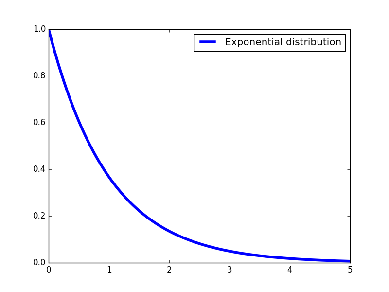
Figure 7: The exponential distribution. Fuzzing the weight of a single vote is done with the exponential distribution. This plot shows the exponential distribution with expected value $1$. A random variable with an exponential distribution may take on any nonnegative real value. The probability of choosing a large value decreases exponentially with that value.

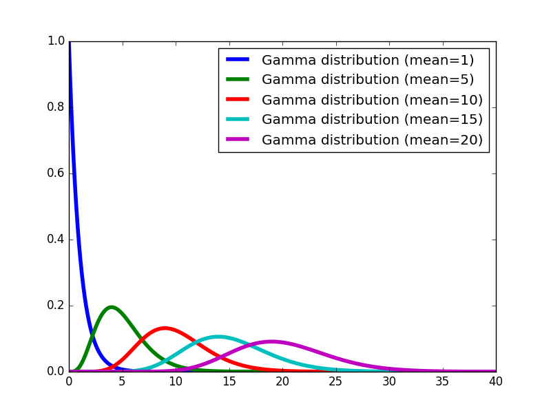
Figure 8: The Gamma distribution. Fuzzing a given count is done with a gamma distribution with expected value equal to the given count (and scale equal to $1$). This plot shows gamma distributions with expected values $1$, $5$, $10$, $15$, and $20$. A gamma distribution with expected value $1$ is the same as the exponential distribution with expected value $1$. A gamma distribution with a given expected value is just the sum of that many independent random variables distributed with the exponential distribution, each having expected value $1$. As the expected value gets larger, the gamma distribution approaches a normal distribution with the same expected value and variance equal to that expected value. The given count for the gamma distribution may be any positive real number, it need not be a whole number.

6.11 Other voting rules

We can now see how the Bayesian audit method applies to any outcome rule.

The main thing to observe is that the outcome rule is applied to each test vote tally to obtain each test instance outcome. The outcome rule might be for an exotic preferential voting method like Schulze’s method, or might be for something as simple as approval voting. All that is needed is that the rule be able to derive a contest outcome from a tally of the number of votes for each possible choice. (For preferential voting, recall that a vote is a list of candidates in order of preference.)

6.12 Generative models and partitioned (stratified) vote sequences

We emphasize that we are using the Bayesian approach to provide a generative model that allows the auditor to generate many test vote tallies that are similar to the unknown actual vote tally.

Mathematically, one may say that we are “sampling from the Bayesian posterior distribution” in the space of vote tallies. The test vote tallies generated are representative of the probability distribution inferred from the known sample of cast votes.

The above observation is central to the handling of both comparison audits and multi-jurisdiction audits.

The following example may be helpful in understanding how this observation gets used for those applications.

Suppose the entire cast vote sequence has been divided arbitrarily into two parts: cast vote sequence part one and cast vote sequence part two.

Suppose further that we have independently sampled from both parts, yielding sample part one and sample part two. (The fraction of votes from each part that are in the corresponding samples need not be the same.)

We assume that there are no CVRs.

We wish to estimate the probability that a particular candidate would win the contest if all cast paper votes were examined by hand.

Using methods described earlier, we can generate many test vote tallies for the cast vote sequence part one based on sample part one, and we can generate many test vote tallies for the cast vote sequence part two based on sample part two, since we have a generative model for each part.

We can now easily generate a test vote tally for the contest as a whole:

• Generate a test vote tally for cast vote sequence part one.

• Independently generate a test vote tally for cast vote sequence part two.

• Add these two test vote tallies for the two parts to obain a test vote tally for the entire contest. (That is, the test vote tally for the entire contest is just the candidate-wise sum of the two test vote tallies for the parts.)

We can in this way generate as many test vote tallies for the entire contest as we like. We can use these test vote tallies to measure “how often a particular candidate wins the contest” just as we did before. We get the answer we seek, even though the cast vote sequence has been broken into parts. We just need to have a generative model for the tallies from each part, and add the test vote tallies from each part to make an overall test vote tally.

This method works because the two parts are independent—the sampling performed in one part is independent of the sampling in the other part.

This approach generalizes in a straightforward way to handle cast vote sequences that have been divided into more than two parts. Such a generalization is useful when a contest is split over multiple jurisdictions, as we shall see.

To be consistent with standard statistics terminology, we may call each “part” a stratum, and the overall approach a kind of stratified sampling [69].

6.13 Bayesian comparison audits

This section describes how a Bayesian comparison audit works. The previous portions of this section described how a Bayesian ballot-polling audit works.

It builds upon and uses the method described above for a Bayesian ballot-polling audit, as extended by the method given in the last subsection above on generative models and partitioned (stratified) vote sequences. The same idea will be used again when we deal with multi-jurisdiction elections.

When CVRs are available, each paper vote has both a reported vote (the choice recorded in the CVR) and an actual vote (the choice seen when examining the paper vote by hand).

When a vote is audited in a comparison audit, both the reported vote and the actual vote are available.

The key idea is to divide the cast vote sequence into parts, or strata, according to the reported votes on the ballots.

For example, the votes with reported choice “Alice” would form one part, while the votes with reported choice “Bob” would form another.

As the audit proceeds, each part will have its own sample, consisting of votes with the same reported choice.

Combining the generated test vote tallies from each part yields a generated test vote tally for the contest as a whole. Once you can generate test vote tallies for the contest as a whole, you can use the Bayesian audit stopping rule to determine when the audit should terminate.

That’s it.

With an accurate scanner, each part (stratum) will consist almost entirely of votes whose actual choice is equal to the reported choice for that part. Exceptions correspond to scanning errors or mis-interpretations. This uniformity, caused by a high correlation between reported and actual choices, is what gives comparison audits increased efficiency. Roughly speaking, one is measuring error rates (which are near zero) rather than vote shares (which may be near one-half); measuring probabilities near zero is easier than measuring probabilities near one-half.

The generative model for a part will thus be a generative model for votes having a given reported choice.

The process of choosing Bayesian priors for comparison audits is discussed further in Appendix B.

Now we can make a generative model for the entire cast vote sequence by combining generative models for each part (i.e., for each reported vote choice).

Each part will have its own sample and nonsample. The generative model will be used to generate test vote tallies for the part, based on the votes in the sample for that part. The test vote tally will have an overall size (number of votes) equal to the number of cast votes having votes with the given reported choice.

Because of the strong (expected) correlation between reported votes and actual votes, we would expect that the generative models for each reported vote would have little variance and be very reliable. It is only when votes with a given reported choice have a variety of corresponding actual votes that the generative model for that reported vote will show much variability.

Combining the generative models for each reported choice gives a generative model for the overall contest. The outcome rule can then be applied to many different test votes tallies for the overall contest, in order to determine the probability that the reported contest outcome is wrong. The Bayesian audit stopping rule can then be used to determine whether the audit should continue or not.

This completes the description of Bayesian comparison audits.

6.14 Workload estimation

As the Bayesian audit proceeds, it is possible to estimate how much work remains to be done (that is, how many votes might yet need to be examined) in a simple manner. (Of course, this is just an estimate, as the actual work to be performed depends on what is found on the votes sampled.)

The method is simple.

Suppose the auditor has audited 400 votes, and computed a probability of 7% that the reported contest outcome is wrong. This 7% estimate is close to his Bayesian risk limit of 5%.

It is easy for the auditor to estimate the probability that the reported outcome is wrong for a sample of 600 votes, for a “likely sample” of that size.

The procedure would first generate examples of the likely extension of the sample (by 200 votes), using Dirichlet parameters from the first 400 and then using a multinomial distribution. (A Polya-Eggenberger distribution might also be used.) Then this hypothetical (larger) sample could be tested to see if it provides sufficient assurance to finish the audit. Running this operation a number of times gives an estimate of the probability that sampling another 200 ballots will allow completion of the audit.

With this information, the auditor might compute that the projected probability that the reported outcome is wrong would almost certainly decrease to 4%, so the audit will be over.

So, the auditor might schedule an escalation of the audit by an additional 200 votes. Or, he could estimate the chances that the audit would be over for sample sizes other than 600.

Of course, he may be unlucky, and the newly audited votes may cause the Bayesian audit to require a total of more than 600 votes to complete. Such is life in the world of statistics.

We note that the auditor can continually monitor his projected workload as the sample size increases.

7 Multijurisdiction (stratified) Bayesian audits

This section explains how one can extend the basic Bayesian audit to handle contests covering multiple jurisdictions.

Example scenario.

For example, suppose that each jurisdiction is a county within a state. While many contests might be county-level, some contests, such one for U.S. Congress, might span several counties.

Suppose each county collects centrally all paper ballots cast in any precinct in the county, and collects together all vote-by-mail ballots sent in by residents of that county. The county scans all such ballots centrally (rather than at the precinct level).

In such a situation, we imagine that each county maintains its own collection of paper ballots and the associated ballot manifest for that collection.

Method.

We now explain how to perform a Bayesian audit in such a situation, for a contest that spans several counties.

The overall structure of the Bayesian audit remains unchanged—we audit until it is decided by a stopping rule that the probability that the reported contest outcome is wrong is less than Bayesian risk limit.

The key idea for handling a contest spanning multiple jurisdictions is simple. Here is the stopping rule to use.

• Use the idea of Section 6.12 to have a generative model for each county. The generative model for a county can produce on demand a large number of “test vote tallies” for the set of all ballots cast in that county, that are consistent with and similar to the tallies for the ballots sampled in that county.

• Combine the generative models for each county to gives an overall generative model for the contest. The overall generative model for the contest can produce on demand a large number of “test vote tallies” for the contest as a whole. Combining the county-level test vote tallies is easily done: they are just added to produce the contest-level test vote tally.

• Use the generative model for the overall contest to estimate the probability that the reported contest outcome is wrong, and thus to determine whether or not to stop the audit.

7.1 Sampling

This section explains how sampling may be arranged for a Bayesian audit of a multijurisdictional contest.

The overall Bayesian audit procedure, like any statistical tabulation audit procedure, has an outer loop involving drawing samples of votes, examining them, and invoking a stopping rule to determine if the audit has finished.

With a multijurisdictional contest, the auditor has to decide whether to sample all jurisdictions at the same rate (proportionate sampling), or whether to accommodate or arrange different sampling rates for for different jurisdictions (disproportionate sampling).

This is a familiar issue with stratified sampling [69]. There are guidelines for some applications, such as “Neyman allocation”, (see e.g. [19]) for deciding how large a sample to draw from each stratum. Those methods do not quite apply here, however, since the outcome rule may be rather arbitrary and since the variances of the fraction of votes for each possible choice are unknown.

Bayesian audits are flexible in this regard, as proportionate sampling is not required. Different jurisdictions may sample votes at different rates, as long as the sampling in various jurisdictions is random and independent of each other.

We envision that some optimization code could be used to plan the sampling strategy. This would allow some counties to be sampled more heavily than others, if this would yield a more efficient audit overall.

Or, each county still having contests-under-audit could continue to examine ballots at the maximum rate of which it is capable of examining ballots, even if this rate varies between counties.

In any case, the flexibility afforded by Bayesian audits enables the county-level results to be smoothly integrated into state-wide risk measurements.

7.2 Mixed contests

The Bayesian approach even applies smoothly in a multijurisdictional setting when some counties do not have CVRs, while others do have CVRs.

One might think that a contest having some counties with no CVRs available would of necessity have to be audited using a ballot-polling approach for all counties (even those that have CVRs). However, the flexibility afforded by Bayesian audits allows one to audit contests having counties of mixed types (where some counties have CVRs and some do not).

The idea is again the same: each county (whether having CVRs or not) has a generative model for test vote tallies for the votes in its county. County-level test vote tallies can be combined to produce a contest-level test vote tally. By producing enough contest-level test vote tallies, the auditor can measure the probability that the reported contest outcome is wrong.

This approach makes sense for states such as Connecticut, where some jurisdictions use scanners while while other jurisdictions hand-counted their paper ballots.

8 Variants

8.1 Multiple contests

Multiple contests can be audited concurrently using these methods.

A “global order” of all ballots can be computed that determines the order in which ballots are sampled. This global order is independent of contest—it might, for example, be determined by a pseudo-random “ballot key” computing by applying SHA256 to the ballot location. Ballots with smaller ballot keys are examined first. This allows the auditing of different contests to be synergistic; a ballot pulled for one contest audit is likely to also be useful for another contest audit.

When a ballot is examined, choices for all relevant (still-being-audited) contests on the same ballot are determined by hand. While each individual contest is being audited independently, for efficiency data collection is performed in parallel—when a ballot is audited all still-being-audited contests are examined and recorded.

Assumption 10

[Concurrent audits share sampled ballots.] We assume that when a ballot is selected by the audit for manual examination, the auditor records the choices made by the voter on that ballot for (at least) all contests under audit.

The audits for the relevant contests make progress in parallel; some may terminate earlier than others.

When all audits have terminated, or all votes have been examined for all contests still being audited, the audit stops.

8.2 Working with sampling rates for different contests

In a multi-contest election, some contests may be landslides, while others may be close.

In a multi-jurisdiction election, the jurisdictions for one contest may include only some of the jurisdictions for another contest.

Our assumption above means that votes for a given contest may be sampled at different rates for different jurisdictions. Even though contest R is not close, there may be a close contest S such that the jurisdictions common to S and R include only some of the jurisdictions for R. The votes in the common jurisdictions may be sampled at a high rate, just for the auditing of contest S. The auditing of contest R in its other jurisdictions may not need to be at such a high rate.

The flexibility of the Bayesian auditing procedure can accommodate such situations, since not all of the jurisdictions for a contest need be sampled at the same rate. Any sampling within a jurisdiction, at any rate, allows a generative model to be created for that race for that jurisdiction. Generative models for different jurisdictions can be combined, even if they were derived from samples produced with different sampling rates.

8.3 Planning sampling rates for different jurisdictions with multiple contests

The sampling rate in a jurisdiction might be determined by the “closest” contest in that jurisdiction. For non-plurality contests, it might be tricky to determine such a “closest” contest.

An extension to the workload estimation method of Section 6.14 may be used to assist with planning the sampling rates for different jurisdictions.

Suppose the audit has already examined a number of ballots in each jurisdiction.

Using this as a basis, one can estimate the probability for each contest that the reported outcome is wrong for various projected sampling rates within the jurisdictions. One can then use optimization methods to estimate how to minimize the total number of ballots that need to be audited in order to complete the auditing of all contests.

The optimization output would specify the estimated number of additional ballots one should audit in each jurisdiction. A search might start with very large sample size for each jurisdiction, which will cause the estimated probability that the reported outcome is wrong for each contest to be below the Bayesian risk limit. Then a simple optimization method that does not use derivatives can be used to repeatedly reduce each jurisdiction’s sample size a bit while maintaining the fact that all contests have estimated probabilities for having incorrect reported outcomes below the Bayesian risk limit. At each point one runs the basic computation of probabilities that the reported outcomes are wrong for each contest (which is at the heart of the Bayesian stopping rule computation). The step size of the optimization would decrease as the optimization proceeds. While this should work, other optimization approaches may be even more efficient.

The discussion of the previous paragraph is altogether too brief; elaborations will be provided in a later version of this note.

9 Discussion

9.1 Open problems

We have not addressed here the situation that some jurisdictions may have collections of paper ballots that are impure with respect to one or more contests. By this we mean that a collection of paper ballots has some ballots containing a contest, and some ballots not containing that contest. For example, a county may receive vote-by-mail ballots, and process them in a way that leaves them unsorted by ballot style. Thus, it may not be possible to efficiently sample ballots containing a particular contest. It is not obvious what the best approach might be for auditing such contests.

9.2 Security

When the tabulation audit spans more than a single precinct, it requires coordination and communication between the various units. Such coordination and communication should be secured, lest the audit process itself become an attack target. This is an area that is not yet well studied in the literature, although standard approaches (e.g. encryption and and digital signatures, public web sites) should apply.

9.3 Pros and Cons

Pros: Bayesian tabulation audits have a number of benefits:

1. Independence of outcome rule. Bayesian audits do not require that the elections be plurality elections. They are “black-box” audit methods: all that is required is that the outcome rule be one that can be applied to a vote tally.

2. Handling of different collection types, or different types of voting systems, even within the same contest. As states move to the next generation of equipment, it may well happen that for a given state-wide contest some collections will have CVRs and some will not. The Bayesian audit methods can easily handle such situations. It can also handle collections that are completely hand-counted. (It is a policy decision as to whether a collection of paper ballots that has already been hand-counted needs to be audited.)

3. Ease of audit management. Since one does not need to sample all collections at the same fixed rate, audit management is simplified. Collections can be guided, but not required, to sample at the same rate.

4. Risk measurement is automatic. Bayesian audit methods automatically provide a measure of the “risk” at each point: the risk is the (posterior) probability that an outcome other than the reported outcome would actually win the contest if/when all ballots are examined by hand.

   If the audit has to “stop early” for some reason (lack of time or resources), you have a meaningful “audit result” to publish, even it it not satisfactorily strong. For example, you might end up saying, “The reported contest winner Alice has an 80% chance of winning according to the posterior, while Bob has a 20% chance of winning. Further sampling would be needed to improve this result. Unfortunately, we did not meet our goal of showing that the reported contest winner has a 95% or better chance of winning according to the posterior.”

5. Reproducibility. Citizens or independent experts can reproduce the simulations and audit computations to verify that the audit was correctly conducted. (Doing so requires having all audit data from the examined ballots, as well as requiring that that all random number generation was performed from public seeds or derived from a public master random audit seed.)

On the other hand, we note the following disadvantages:

1. Simulation-based: Interpreting the sampled votes to derive the audit conclusions requires some software and computer time. However, the software can be written by any third party and publicly disclosed for anyone to use. The computation required is cheap, compared to the manual labor required to retrieve and interpret ballots.

2. Math: These methods requires a bit of math and statistics to understand. But this is true for any statistical tabulation audit.

10 Related work

Chilingirian et al. [8] describe the design, implementation, and testing of an audit system based on the use of Bayesian audits for the Australian 2016 Senate elections. Because of the complexity of the Australian voting system [66], the “black box” character of Bayesian election audits was especially appealing. Unfortunately, the Australian Election Commission decided not to proceed with the actual audit (probably for political rather than technical reasons).

A statistical tabulation audit may be viewed as a sequential decision-making procedure as described by Wald [62, 63].

Appendix A Appendix A. Election complexities

Elections can be complicated, and audits, which aim to check the correctness of a election contest outcomes, inherit that complexity. Such complexity derives from having:

• multiple contests,

• multiple candidates per contest (with voters perhaps allowed to write-in candidates not otherwise listed on the ballot)

• multiple modes of casting paper ballots (in-person, vote-by-mail (VBM), voting with drop-off boxes), with some vote-by-mail ballots possibly arriving several days late but still within the deadline for acceptance,

• multiple administrative jurisdictions (state, counties, cities, precincts, other),

• contests spanning some jurisdictions and not others,

• multiple types of equipment (for example, some scanners produce one electionic cast vote record (CVR) per vote scanned, while other scanners only produce tallies per candidate of votes scanned),

• a variety of methods for organizing and storing the cast paper ballots, including those that mix together ballots of various ballot styles

• some elections having so many contests that a single ballot may need to be printed on two or more separate cards,

• limited resources and tight deadlines,

• the nature of most statistical audit methods to have resource and time requirements that have considerable variability (from looking at just a handful of votes in a landslide contest to hand-counting of all cast paper votes in a very close contest),

• statistical audit methods that may be relatively sophisticated and difficult to understand, even if easy to apply,

• statistical audit methods that are sequential decision-making in flavor, requiring dynamic real-time computations during the audit (even if simple) to decide when to stop the audit,

• statistical audit methods requiring the coordination of sampling and hand-examination of a number of widely separated collections of paper votes,

• the possible need for custom software just to support the audit,

• a need to provide transparency while protecting the privacy of voters’ choices, and

• a need to provide straightforward evidence that the contest outcome(s) are correct, while accomodating these complexities.

Appendix B Appendix B. Math

This appendix gives some mathematical details, clarifications, and elaborations of the Bayesian audit method presented above. We follow the notational conventions of Rivest and Shen [44]; see that paper for more detailed notation and discussions.

We assume here that we are dealing with just a single contest in a single jurisdiction.

B.1 Notation

Here we restrict attention to a single contest.

Number of cast votes

Notation 1

We let $n$ denote the total number of cast votes in the contest.

Number of possible choices for a vote

Notation 2

We let $t$ denote the number of possible choices a paper vote may exhibit.

This is the number of possibilities for an “actual vote”—what a manual examination of the paper ballot would reveal. It may be the actual vote is “invalid” or “overvote” or “undervote” or the like, so that the number $t$ of possible choices might be slightly larger than needed to cover just the possible valid votes.

We identify the $t$ possible votes with the integers $1,2,\ldots,t$.

With plurality voting on $m$ candidates, there are $t=m$ possible votes (possibly plus one or two for undervotes or invalid votes), and $M=m$ possible contest outcomes.

With preferential or ranked-choice voting, each cast vote provides a listing of the $m$ candidates in some order, so there are $t=m!$ possible votes (plus one or two for invalid votes), but only $M=m$ possible contest outcomes.

Vote sequences

We denote the (overall actual) vote sequence of cast votes (for a single jurisdiction) as

$$\bm{a}=\{a_{1},a_{2},\ldots,a_{n}\}\ ,$$

where each $a_{i}$ is a vote (an integer in $\{1,2,\ldots,t\}$).

The vote sequence is best viewed as a sequence rather than as a set, since there may be repeated items (identical votes), and we may need to index into the sequence to select random votes for auditing.

Tallies

If $\bm{a}$ is a vote sequence, we let

$$\mbox{tally}(\bm{a})=\bm{A}=(A_{1},A_{2},\ldots,A_{t})$$

denote the tally of $\bm{a}$, giving for each $i$ the number $A_{i}$ of cast votes for choice $i$. The sum of the tally elements is equal to $n$, the number of cast votes.

Similarly, we let

$$\mbox{voteshare}(\bm{a}) = (A^{\prime}_{1},A^{\prime}_{2},\ldots,A^{\prime}_{t})$$

$$= (A_{1}/n,A_{2}/n,\ldots,A_{t}/n)$$

denote the voteshare of $\bm{a}$, giving the fraction $A^{\prime}_{i}$ of cast votes for each possible choice $i$. The sum of the voteshares is equal to 1.

B.2 Probability distributions

The auditor can represent his uncertainty as a probability distribution over possible vote sequences containing the correct number of cast votes.

We assume that a tally is a sequence of $t$ nonnegative integers that sum to $n$.

Dirichlet-multinomial distributions

The approach given here is modeled on the use of a Dirichlet-multinomial distribution, a rather standard approach. Such distributions are frequently used in machine learning; see Murphy [30].

We use multivariate Dirichlet-multinomial distributions to model the auditor’s information and uncertainty about the voteshares for the vote sequence (which is really all about his uncertainty about the voteshares in the nonsample).

Such distributions are Dirichlet on the multinomial probabilities, then multinomial on the counts.

We denote the Dirichlet hyperparameters as

$$\bm{\alpha}=(\alpha_{1},\alpha_{2},\ldots,\alpha_{t})\ .$$

These hyperparameters are nonnegative real values. There are $t$ hyperparameters, one for each of the possible votes for the contest being audited.

For a given vector of hyperparameters $\bm{\alpha}$, the Dirichlet distribution is a probability distribution over the simplex $S_{t}$ of $t$-tuples of nonnegative real numbers adding up to $1$. In our case, the Dirichlet distribution is a probabilistic model of the multinomial probabilities defined on the set of choices.

The mean of the Dirichlet distribution is $(x_{1},x_{2},\ldots,x_{t})$, where $x_{i}=\alpha_{i}/\sum_{i}\alpha_{i}$. That is, the mean voteshare for choice $i$ is proportional to $\alpha_{i}$, normalized so that the $x_{i}$ values add up to $1$.

B.3 Prior probabilities

The choice of prior is always an interesting one for a Bayesian.

Since we are using a Dirichlet distribution to represent what the auditor knows about the voteshares for the cast vote sequence, the prior probability distribution is defined by the choice of the Dirichlet hyperparameters. Choosing a prior is done by choosing the initial set of hyperparameters for the Dirichlet distribution.

In this subsection we discuss the choice of prior, noting that one may wish to take some different approaches for ballot-polling Bayesian audits and for comparison Bayesian audits.

In the main body of this note, we avoiding talking about prior distributions, effectively setting to zero all of the hyperparameters for the prior. Having all hyperparameters set to zero yields the Haldane prior, which is a reasonable choice for ballot-polling audits when the initial sample size is not too small. As we now discuss, other choices may also be reasonable, even for a ballot-polling audit. And different choices may be best for a comparison audit.

A Bayesian has an initial (or prior) “belief state” represented as his prior probability distribution on the set of possible voteshare distributions. Once he sees data (the sample of cast votes seen in the audit), he updates his belief state, using Bayes Rule, to become his final (or posterior) distribution.

With a Dirichlet distribution, this update is exceptionally simple. The initial distribution is represented by the initial hyperparameters, one per possible choice for the contest. These initial hyperparameters are commonly viewed as “pseudocounts,” for reasons that will become immediately clear. When a sample is examined, each hyperparameter is increased by the count of the number of times its corresponding choice is seen in the sample [30, Section 3.4]. The resulting set of hyperparameters defines the final (or posterior) Dirichlet distribution.

For example, suppose we have a contest between Alice and Bob, and suppose further that a Bayesian observer has initial hyperparameters of 5 for Alice and 6 for Bob. The observer then sees a random sample of cast votes having 10 votes for Alice and 15 votes for Bob. The observer’s posterior distribution then has hyperparameters of 15 for Alice and 21 for Bob.

The initial hyperparameters (“pseudocounts”) behave just like “virtual sample counts.” If you start with a Haldane prior (initial hyperparameters equal to 0) and see a sample with 10 votes for Alice and 15 votes for Bob, you end up with final hyperparameters of 10 for Alice and 15 for Bob. If instead we set the initial hyperparameters to 10 for Alice and 15 for Bob, we achieve the same result, without having seen any sample. In this way the initial hyperparameters can be viewed as representing the observer’s degree of belief about the possible distribution of voteshares as equivalent to the observer having seen a “virtual sample” of cast votes.

The final hyperparameters for one stage of the audit become the initial hyperparameters for the next stage of the audit, so the hyperparameters act during the audit as counters for the number of votes seen for each possible choice, where these counters have initial values set equal to the initial hyperparameters.

The reader may be concerned that biasing the initial hyperparameters in favor of one candidate or another may be like “stuffing the ballot box”—making it seem more likely that one candidate or another appears to be winning the contest. This is a valid concern. We therefore require that the auditor use “neutral” initial hyperparameters–ones that give equal weight to each choice capable of winning the contest.

The initial hyperparameters do not need to give an equal weight for choices that can’t win the contest. For example, the initial hyperparameters might give Alice and Bob each hyperparameters equal to $2$, while giving “undervote” a hyperparameter equal to $0$.

The intuition that the initial hyperparameters correspond to the observer having seen a “virtual sample” of the data is also a good one in the following sense: as the hyperparameters increase in value, the Dirichlet distribution becomes more tightly concentrated about its mean. A Dirichlet distribution with hyperparameters of 10 for Alice and 20 for Bob has the same mean as one with hyperparameters of 100 for Alice and 200 for Bob, which is the point where Alice gets 1/3 of the voteshare and Bob gets 2/3. But the second Dirchlet distribution has smaller variance in the voteshare parameters. This makes sense, as more sample data makes for better estimates.

Let us call the sum of the initial hyperparameters the “initial size” (of the hyperparameters), and let us call the number of cast votes in a sample the “sample size.” We call them both “size” since they are comparable measures: one of the strength of the initial belief, and the other of the strength of the data.

As he increases the initial size, the Bayesian is giving greater weight to his initial beliefs. As he increases the sample size, the Bayesian is giving greater weight to the observed data. Eventually, with enough data, the sample overwhelms any initial beliefs.

Choosing a Dirichlet prior distribution (that is, the initial hyperparameters) may be done in a two-step manner:

1. [Choose initial size.] Choose the initial size of the hyperparameters (that is, their sum) to reflect the desired strength of initial belief.

2. [Choose individual hyperparameters.] Allocate the initial size among the individual hyperparameters to reflect the initial expectations for the corresponding voteshares. (For a Bayesian audit, however, the individual hyperparameters for all possibly-winning choices must be set equal to each other, so as not to bias the audit.)

For example, an auditor might choose initial hyperparameters of $1$ each for Alice and Bob, and $0$ for “undervote.” This choice of hyperparameters has an initial size of $2$—the auditor is saying that his prior distribution is fairly weak and that it is unbiased.

For a Bayesian audit, it makes sense to have a weak prior (that is, with a small initial size). The audit should be governed primarily by the data, and not by the prior. Even if all of the candidates have equal initial hyperparameters, having large hyperparameter values would slow down the audit by requiring the sample to be correspondingly larger.

One reason for choosing nonzero initial hyperparameters is that if a hyperparameter for candidate X is zero, that component of the Dirichlet distribution is initially set to zero as well. That is, the initial distribution effectively assumes that candidate X won’t be getting any votes at all. When the hyperparameter is positive, the distribution assumes that the candidate will be getting votes in proportion to its hyperparameter. If every candidate may get some votes, then nonzero hyperparameters for the candidates is reasonable.

A common choice for Bayesian inference is to use a Jeffreys prior, which sets each hyperparameter to 1/2. The initial size of this hyperparameter setting is $t/2$. We can recommend this choice for plurality elections.

The Haldane prior, which sets all initial hyperparameters to zero, is another reasonable choice, and is the one described in the body of this note. I suggest that its use is reasonable as long as the initial sample size is large enough so that candidates who reasonably might win the contest obtain some votes in the initial sample.

We note that this is known as an improper prior (a term of art in the field), but using such improper priors within a Bayesian framework is not unusual. A Haldane prior is simplest prior to implement.

One reason the Haldane prior is attractive is that it works smoothly when there are large number of possible choices for a vote, such as for preferential voting.

Using the Haldane prior here may also be viewed as an application of the commonly-used empirical Bayes method, wherein parameters defining the prior distribution are inferred from the sample rather than chosen before seeing any data.

The pilot study of auditing the Australian Senate elections [8] used the empirical Bayes method in this manner.

Priors for Bayesian comparison audits.

How should one set up a Bayesian prior for a comparison audit?

As described in Section 6.13, a Bayesian comparison audit tallies (reported vote, actual vote) pairs, where the reported vote is from the CVR and the actual vote is from the hand examination of the corresponding paper ballot.

If there are $t$ choices possible for a contest (including the non-candidate choices such as “undervote”), then there are $t^{2}$ tallies being kept by the audit, one for each possible such pair of (reported vote, actual vote). We may think of these tallies as forming a matrix, with one row for each possible reported vote and one column for each possible actual vote.

There will also be $t^{2}$ hyperparameters, one for each tally position—that is, one hyperparameter for each position in the tally matrix. The hyperparameters may be viewed as initial “pseudocounts” as before for the tallies.

The diagonal of the tally matrix gives the counts for votes read without error—where the reported vote is equal to the actual vote. The off-diagonal elements give counts for votes read with error—where the reported vote is not equal to the actual vote.

The principle of neutrality means that the hyperparameters along the diagonal should all be equal—no candidate is believed initially to be more likely to win the contest.

As described in Section 6.13, the Bayesian comparison audit proceeds as if it were $m$ separate audits—one for each possible reported vote.

The tally matrix is split up row-wise into $m$ separate rows, each row giving the tally for its own subaudit (where all of the reported votes are equal).

The voteshare distribution for a given row will be highly skewed. We expect one entry (from the diagonal) to have the overwhelming majority of the votes, while the others (from off-diagonal) to have tiny tallies.

A reasonable hyperparameter setting in such a case might be to use $50$ for the hyperparameter for the on-diagonal cell, and to use $0.5$ (or some other small value) for the off-diagonal elements.

These values may be chosen so that:

• The sum of all the entries in the initial tally matrix is roughly the number of votes for which the auditor feels that the evidence (votes examined and interpreted by hand) should begin to balance out the prior.

• The ratio of the sum of the off-diagonal elements to the diagonal element should be roughly equal to (or a bit greater than) the expected error rate in the ballots examined. For example, with a two-candidate race, the ratio 0.5/50 = 0.01 corresponds to a prior estimate of an error rate of one percent.

We note that

• Although these pseudocounts affect the tallies as seen by the audit, they are symmetric with respect to the candidates. Thus these pseudocounts do not favor any one candidate over another.

• The pseudocounts ”smooth out” the tallies when the sample sizes are small, by blending the pseudocounts with the actual counts seen during the audit. For example, if the audit had examined two ballots, both of which were ”Yes” ballots, one shouldn’t conclude that the voting was unanimously for ”Yes”! With the pseudocounts added in, the voting appears to the audit as 52/50, where Yes has 52 votes and No has 50. Clearly more auditing needs to be done to tell the difference now!

• The sum of all the pseudocounts in the matrix (in this case 50+1+1+50=102) determines how much the prior is weighted compared to the new audit data. In this case, it will take about 102 ballots examined to have as much weight as the prior has been given by the pseudocounts.

Priors for preferential voting.

Priors for preferential voting are more complicated, as there are $m!$ different possible orderings of $m$ candidates. When $m$ is even modestly large (e.g., $m=10$) the number of possible votes becomes very large.

For both ballot-polling and comparison audits, the simplest approach is to stick with a Haldane prior, which gives a $0$ hyperparameter to each possible ordering.

Parallel audits.

Rivest and Shen [44] also give another approaches to using priors. It is possible run several statistical tabulation audits in parallel: they all use the same sample data, but have different stopping rules. They suggest that one could use not only a neutral prior (such as the Jeffreys prior or the Haldane prior), but also one prior biased in favor of each candidate (that is, with a larger initial hyperparameter for that candidate). A losing candidate may need to be convinced that the voters really elected someone else by seeing that the data swamps even a prior biased in favor of that losing candidate. The audit stops when all subaudits (with different priors) have terminated. (Note: parallel audits should not be confused with parallel testing [21].)

B.4 Updates with Bayes Rule

Bayes rule is used to update the hyperparameters by adding the sample tally to the prior hyperparameters, as usual. The Haldane prior sets all of the initial hyperparameters equal to zero, which simplifies things, so that after update the Dirichlet hyperparameters are just the tallies for the current sample.

B.5 Generating test nonsample tallies

When we “sample the posterior” we mean sampling from the Dirichlet distribution defined by the Dirichlet hyperparameters after they have been updated by Bayes Rule using the observed data. In our case, since we are using the Haldane prior, these hyperparameters are just the tallies for the observed sample. The sample from the Dirichlet distribution is a test multinomial probability distribution—a set of nonnegative real numbers adding up to one. Since our goal here is to generate a test nonsample tally, we draw a number of (simulated) ballots equal to the (known) size of the nonsample, where each ballot has a vote selected at independently at random from the set of available options according to the multinomial probability distribution computed earlier. The tally of these votes gives us our test nonsample tally.

Sampling from a Dirichlet distribution

A standard method to generate a multivariate random variable distributed according to a Dirichlet distribution with hyperparameters $(\alpha_{1},\alpha_{2},\ldots,\alpha_{n})$ is as follows:

1. For each $i$, $1\leq i\leq t$, generate a random variable $x_{i}$ distributed according a gamma distribution with shape parameter $\alpha_{i}$ and scale parameter $1$ [67].

2. Normalize these values so their sum is one. That is, replace each $x_{i}$ by $x_{i}/v$ where $v$ is the sum of the original $x_{i}$ values.

An important property of gamma distributions is that a random variable distributed according to gamma distribution with shape parameter $k$ and scale parameter $1$ has expected value $k$ and variance $k$.

This property motivates our presentation of “fuzzing” above in Section 6.10 where a sample tally equal to $k$ is replaced by a random variable distributed according to a gamma distribution with shape $k$ and scale $1$.

It is interesting to note that the gamma distribution with shape parameter one and scale parameter $1$ is just an exponential distribution with expected value $1$.

A gamma distribution does not need to have a shape parameter that is a whole number; it may be any nonzero real value.

Furthermore, a gamma distribution with shape parameter $k$ and scale parameter $1$ is just the sum of $k$ exponential distributions each having expected value one. In general, a gamma distribution with shape parameter $k$ and scale parameter $1$ is the sum of any finite set of gamma distributions with scale parameter $1$ if their shape parameters add up to $k$.

This motivates our perspective, also presented in Section 6.10, of viewing “fuzzing” as replacing the weight (originally one) of each vote with a random variable drawn according to an exponential distribution with expected value one. It is entirely equivalent to replacing tallies with the corresponding gamma-distributed random variables.

Alternatives

One might reasonably consider alternatives to fuzzing that use something other than gamma-distributed random variables.

The most significant properties of the gamma distribution (with shape parameter $k$ and scale factor $1$) here are that it has mean $k$ and variance $k$.

A variable distributed according to a gamma distribution is nonnegative, which seems a natural property for our purposes. However, non-negativity doesn’t seem required (see discussion below on the use of the normal distribution for fuzzing).

We now present some alternative methods for fuzzing the sample counts. These methods may be viewed as good and perhaps amusing heuristic approximations to the use of the gamma distribution. They are perhaps best for pedagogic use—the shuffle-and-cut variation is really easy to explain.

Alternatives worth considering include:

• Using a Binomial distribution with mean $k$ and probability $p=1/2$, scaled up by a factor of two. This gives values that are nonnegative even integers between zero and $2k$; the mean and variance are both equal to $k$. This (scaled) binomial distribution is identical to the sum of $k$ (scaled) Bernouli random variables, so we can view the fuzzing operation here as replacing each ballot’s initial weight of one with either 2 or 0, according to a fair coin flip. (“Double or nothing” for each ballot’s weight.) Equivalently, to obtain a fuzzed sample merely delete each ballot in the sample with probability 1/2, and replace it with two copies of itself with probability 1/2. Another simple variant on this idea is to “shuffle and cut”: randomly shuffle (re-order) the sample, then cut it into two halves. Tally the first half. Double the tallies to achieve an expected value and variance of $k$ for each choice that occurs $k$ times in the original sample.

• Using a normal distribution with mean and variance both equal to $k$. Using the normal distribution has many appealing features; it is well-studied, is its own conjugate, is additive, and (by the central limit theorem) represents the asymptotic limit of many other distributions. While it may result in fuzzed values that are negative, I don’t see how this causes any problems for us, particularly if we are using the “small sample assumption.” Using the normal distribution may be viewed as a continuous variant of the binomial distribution given above.

  (Most outcome rules also work fine if some input tallies are negative numbers, since the rules typically work by comparing tallies with each other, or by comparing sums of tallies with sums of other tallies.)

• Using a Poisson distribution with mean $k$ (which also has variance $k$). This gives values that are nonnegative integers. It is also additive, so that one could view the fuzzing on a per-ballot basis, where a ballot’s initial weight of one is replaced by a random variable drawn according to a Poisson distribution with expected value one.

• Using a negative binomial distribution with parameters $k$ and $p=1/2$; The probability of value $i$ is probability of flipping a fair coin and seeing $i$ heads before you see $k$ tails. This has integer values with expection $k$ and variance $2k$. It is also additive, so one could view the fuzzing on a per-ballot basis, where a ballot’s initial weight of one is replaced by the number of fair coin flips seen showing heads before the first tail is seen. The implications of the higher variance for the negative binomial need study.

• Using a Polya-Eggenberger distribution defined by Polya’s Urn model. (See Rivest and Shen [44] and Rivest [42].)

Interesting as these are, we prefer the use of the gamma distribution for its familiarity, efficiency, and ability to handle small non-integral counts as inputs.

The gamma, normal, and Poisson distributions all share this last feature—that their distributions may have a mean that is a small real number. This feature might be of interest when creating a prior for comparison audits, where a prior for the errors may be based on the prior belief that errors will be rare.

Another related approach worth mentioning here is bootstrapping, a popular statistical method (see Efron [10, 11, 12]) that has also been suggested for tabulation audits (see Rivest and Stark [45]). Here a sample of size $s$ is transformed into a test sample of size $s$ by sampling from the original sample with replacement. The test sample tally can then be scaled to yield a test nonsample tally as usual. The statistics are very close to those obtained by using the Poisson distribution. Bootstrapping is very easy to implement, although the resampling takes time proportional to the size $s$ of the sample rather than the length $t$ of the tally.

These alternative methods are good approximations to the use of gamma-distributed random variables. However, they can presumably stand on their own merits as fully-justified Bayesian audits, with appropriately chosen prior distributions.

Small sample assumption.

We now present another simplification of the Bayesian method for use when the sample size is very small compared to the nonsample size. We call this the “small sample assumption.” This situation is the typical one when when contests are not close.

In the small sample case, one may reasonably skip the step of adding the sample tally to the test nonsample tally, and just use the test nonsample tally directly.

We can implement a Bayesian audit stopping rule under the small sample assumption by examining the contest outcomes for many fuzzed versions of the sample tally (without scaling).

An approach based on the small sample assumption provides an approximate Bayesian foundation and justification for several of the “black-box audits” proposed by Rivest and Stark [45]).

B.6 Implementation note

Computing gamma variates: Spreadsheet

We note that computing random variables distributed according to a gamma distribution is very easy. For example, the following formula gives a cell in your spreadsheet a random value distributed according to a gamma distribution with shape parameter $k$ and scale parameter $1$:

$$\texttt{=GammaInv(Rand(),k,1)}\ .$$

Computing gamma variates: Python

In Python, the line

x = numpy.random.gamma(k,1,t)

generates a vector $x$ of $t$ independent random variates, each distributed in accordance with a gamma distribution with shape parameter $k$ and scale factor $1$.

Similarly, in Python it is easy to compute an array of $t$ random variables each equal to two times a binomial random variable with mean $k/2$ and probability $p=1/2$:

x = 2*numpy.random.binomial(k,0.5,t)

Software for Bayesian audits

Open-source code implementing and illustrating Bayesian audits is available on github .

Code for Bayesian audits that was developed for potential use in the 2016 Australian Senate elections is described by Chilingirian [8], and is available on github .

B.7 Accuracy

The number of “test vote tallies” that need to be generated depends on how much accuracy you may wish to have in the computation of the probability that the reported contest outcome is wrong. We recommend using 1,000,000 test vote tallies for high accuracy, although a Bayesian audit may work well with many fewer (say 1,000).

B.8 Relation to frequentist risk-limiting audits

Standard risk-limiting audits are based on the Wald’s Sequential Probability Ratio Test. It is interesting to note that such methods can be viewed as Bayesian methods—see, for example, Berger [4]. We omit details here.

References

- [1] R. Michael Alvarez, Lonna Atkeson, and Thad E. Hall. Confirming Elections: Creating Confidence and Integrity through Election Auditing. Palgrave Macmillan, 2012.
- [2] Javed Aslam, Raluca A. Popa, and Ronald L. Rivest. On auditing elections when precincts have different sizes. In D. Dill and T. Kohno, editors, Proc. 2008 USENIX/ACCURATE Electronic Voting Technology Workshop. USENIX/ACCURATE, 2008. See http://www.usenix.org/events/evt08/tech/full_papers/aslam/aslam.pdf.
- [3] J. Benaloh, D. Jones, E. Lazarus, M. Lindeman, and P.B. Stark. SOBA: Secrecy-preserving observable ballot-level audit. In Proceedings 2011 Electronic Voting Technology Workshop/Workshop on Trustworthy Elections (EVT/WOTE ’11), 2011. http://static.usenix.org/events/evtwote11/tech/final_files/Benaloh.pdf.
- [4] James O. Berger. Statistical Decision Theory and Bayesian Analysis. Springer, 2010.
- [5] Steven Brams. Mathematics and Democracy: Designing Better Voting and Fair-Division Procedures. Princeton, 2008.
- [6] J. Bretschneider, S. Flaherty, S. Goodman, M. Halvorson, R. Johnston, M. Lindeman, R.L. Rivest, P. Smith, and P.B. Stark. Risk-limiting post-election audits: Why and how?, Oct. 2012. (ver. 1.1) http://people.csail.mit.edu/rivest/pubs.html#RLAWG12.
- [7] S. Checkoway, A. Sarwate, and H. Shacham. Single-ballot risk-limiting audits using convex optimization. In D. Jones, J.-J. Quisquater, and E. Rescorla, editors, Proceedings 2010 EVT/WOTE Conference. USENIX/ACCURATE/IAVoSS, August 2010.
- [8] Berj Chilingirian, Zara Perumal, Ronald L. Rivest, Grahame Bowland, Andrew Conway, Philip B. Stark, Michelle Blom, Chris Culnane, and Vanessa Teague. Auditing Australian Senate ballots. CoRR, abs/1610.00127, 2016. arxiv.org/abs/1610.00127.
- [9] U.S. Congress. Help America Vote Act of 2002 . https://www.eac.gov/assets/1/6/HAVA41.PDF, 2002.
- [10] B. Efron. Bootstrap methods: Another look at the jackknife. Annals of Statistics, 7(1):1–26, 1979.
- [11] Bradley Efron. The Jackknife, the Bootstrap, and Other Resampling Plans. SIAM, 1982. No. 38 in CBMS-NFS Regional Conference Series in Applied Math.
- [12] Bradley Efron and R.J. Tibshirani. An Introduction to the Bootstrap. Chapman & Hall / CRC, 1993. Monographs on Statistics and Probability 57.
- [13] FairVote. Better elections are possible. http://www.fairvote.org/.
- [14] Overseas Vote Foundation. The future of voting: End-to-end verifiable internet voting — specification and feasibility study. (I was on the Advisory Council for this report.).
- [15] San Francisco. June 2016 1% manual tally - dice. https://www.youtube.com/watch?v=Sufb7ykByWA.
- [16] San Francisco. Random selection of the 1% for manual tally - June 2016. https://www.youtube.com/watch?v=sdWL8Unz5kM.
- [17] Eric Geller. Online voting is a cybersecurity nightmare. Daily Dot, June 10 2016. https://www.dailydot.com/layer8/online-voting-cybersecurity-election-fraud-hacking/.
- [18] J. L. Hall, L. W. Miratrix, P. B. Stark, M. Briones, E. Ginnold, F. Oakley, M. Peaden, G. Pellerin, T. Stanionis, and T. Webber. Implementing risk-limiting post-election audits in California. In Proc. 2009 Electronic Voting Technology Workshop/Workshop on Trustworthy Elections (EVT/WOTE ’09, Montreal, Canada). USENIX, Aug 2009. http://www.usenix.org/event/evtwote09/tech/full_papers/hall.pdf.
- [19] H. F. Huddleston, P. L. Claypool, and R. R. Hocking. Optimal sample allocation to strata using convex programming. Journal of the Royal Statistical Society (Series C), 19(3):273–278, 1970.
- [20] K. Johnson. Election verification by statistical audit of voter-verified paper ballots. http://ssrn.com/abstract=640943, Oct. 31 2004.
- [21] Douglas Jones. The Machinery of Democracy: Protecting Elections in an Electronic World, chapter Voting Machine Testing (Appendix E). Voting Right and Elections. Brennan Center for Justice (NYU School of Law), June 27, 2006. http://homepage.divms.uiowa.edu/~jones/voting/testing/#parallel.
- [22] Douglas W. Jones. On optical mark-sense scanning. In D. Chaum et al., editor, Towards Trustworthy Elections, volume 6000 of Lecture Notes in Computer Science, pages 175–190. Springer, 2010. See http://www.cs.uiowa.edu/~jones/voting/OpticalMarkSenseScanning.pdf.
- [23] Douglas W. Jones. A brief illustrated history of voting. http://homepage.divms.uiowa.edu/~jones/voting/pictures/, 2013.
- [24] Douglas W. Jones and Barbara Simons. Broken Ballots: Will Your Vote Count? Center for the Study of Language and Information, 2012.
- [25] M. Lindeman, M. Halvorseon, P. Smith, L. Garland, V. Addona, and D. McCrea. Principle and best practices for post-election audits. www.electionaudits.org/files/best%20practices%20final_0.pdf, 2008.
- [26] Mark Lindeman and Philip B. Stark. A gentle introduction to risk-limiting audits. IEEE Security and Privacy, 10:42–49, 2012.
- [27] Mark Lindeman, Philip B. Stark, and Vincent S. Yates. BRAVO: Ballot-polling risk-limiting audits to verify outcomes. In Alex Halderman and Olivier Pereira, editors, Proceedings 2012 EVT/WOTE Conference, 2012.
- [28] Randall Munroe. Frequentists vs. Bayesians . https://www.explainxkcd.com/wiki/index.php/1132:_Frequentists_vs._Bayesians, Nov. 9, 2012.
- [29] Randall Munroe. What If?: Serious Scientific Answers to Absurd Hypothetical Questions. Houghton Mifflin, 2014. See https://what-if.xkcd.com/19/ for discussion of ties.
- [30] Kevin P. Murphy. Machine Learning: A Probabilistic Perspective. MIT Press, 2012.
- [31] C. Andrew Neff. Election confidence: A comparison of methodologies and their relative effectiveness at achieving it. www.verifiedvoting.org/downloads/20031217.neff.electionconfidence.pdf, 2003.
- [32] Lawrence Norden, Aaron Burstein, Joseph Lorenzo Hall, and Margaret Chen. Post-election audits: Restoring trust in elections. Technical report, Brennan Center for Justice and Samuelson Law, Technology & Public Policy Clinic, 2007.
- [33] National Institute of Standards and Technology (NIST). NIST randomness beacon. https://beacon.nist.gov/home.
- [34] National Institute of Standards and Technology (NIST). Secure hashing. http://csrc.nist.gov/groups/ST/toolkit/secure_hashing.html, 2015.
- [35] National Institute of Standards and Technology (NIST). Random bit generation. https://csrc.nist.gov/Projects/Random-Bit-Generation, 2017.
- [36] California Secretary of State. Post-election risk-limiting audit pilot program, 2011-2013. http://www.sos.ca.gov/elections/voting-systems/oversight/post-election-auditing-regulations-and-reports/post-election-risk-limiting-audit-pilot-program/.
- [37] Colorado Secretary of State. Determination of voter intent. www.sos.state.co.us/pubs/elections/docs/voterIntentGuide.pdf, September 8, 2017.
- [38] Colorado Secretary of State Wayne Williams. Audit center. https://www.sos.state.co.us/pubs/elections/auditCenter.html, 2017.
- [39] Jeremy Orloff and Jonathan Bloom. Comparison of frequentist and Bayesian inference. Course notes for MIT course 18.05 Spring 2014, Class 20. Available at: https://ocw.mit.edu/courses/mathematics/18-05-introduction-to-probability-and-statistics-spring-2014/readings/MIT18_05S14_Reading20.pdf, 2014.
- [40] Ronald L. Rivest. On the notion of ‘software independence’ in voting systems. Philosophical Transactions of The Royal Society A, 366(1881):3759–3767, August 6, 2008.
- [41] Ronald L. Rivest. Reference implementation code for pseudo-random sampler. https://people.csail.mit.edu/rivest/sampler.py, 2011.
- [42] Ronald L. Rivest. How to Check Election Results (feat. Polya’s Urn) . YouTube Numberphile interview by Brady Haran., November 7, 2016. Available at https://www.youtube.com/watch?v=ZM-i8t4pMK0.
- [43] Ronald L. Rivest. ClipAudit—a simple post-election risk-limiting audit. https://arxiv.org/abs/1701.08312, 2017.
- [44] Ronald L. Rivest and Emily Shen. A Bayesian method for auditing elections. In J. Alex Halderman and Olivier Pereira, editors, Proceedings 2012 EVT/WOTE Conference, 2012. Available at https://www.usenix.org/conference/evtwote12.
- [45] Ronald L. Rivest and Philip B. Stark. Black-box post-election audits. (Available from authors.).
- [46] Ronald L. Rivest and John P. Wack. On the notion of “software independence” in voting systems. Prepared for the TGDC, and posted by NIST at the given url.
- [47] Roy G. Saltman. The History and Politics of Voting Technology: In Quest of Integrity and Public Confidence. Palgrame Macmillan, 2006.
- [48] A. D. Sarwate, S. Checkoway, and H. Shacham. Risk-limiting audits and the margin of victory in nonplurality elections. Politics and Policy, 3(3):29–64, 2013.
- [49] P. B. Stark. Risk-limiting vote-tabulation audits: The importance of cluster size. Chance, 23(3):9–12, 2010.
- [50] P. B. Stark and D. A. Wagner. Evidence-based elections. IEEE Security and Privacy, 10(05):33–41, Sep-Oct 2012.
- [51] Philip B. Stark. Conservative statistical post-election audits. Ann. Appl. Stat., 2:550–581, 2008.
- [52] Philip B. Stark. A sharper discrepancy measure for post-election audits. Ann. Appl. Stat., 2:982–985, 2008.
- [53] Philip B. Stark. CAST: Canvass audits by sampling and testing. IEEE Trans. Inform. Forensics and Security, 4(4):708–717, Dec. 2009.
- [54] Philip B. Stark. Efficient post-election audits of multiple contests: 2009 California tests. ssrn.com/abstract=1443314, 2009. 2009 Conference on Empirical Legal Studies.
- [55] Philip B. Stark. Risk-limiting post-election audits: P-values from common probability inequalities. IEEE Trans. on Information Forensics and Security, 4:1005–1014, 2009.
- [56] Philip B. Stark. Super-simple simultaneous single-ballot risk-limiting audits. In Proc. 2010 EVT/WOTE Workshop, 2010. http://www.usenix.org/events/evtwote10/tech/full_papers/Stark.pdf.
- [57] Philip B. Stark. Tools for comparison risk-limiting election audits. http://www.stat.berkeley.edu/~stark/Vote/auditTools.htm, 2015.
- [58] Philip B. Stark and Vanessa Teague. Veriable european elections: Risk-limiting audits for d’hondt and its relatives. USENIX Journal of Election Technology and Systems (JETS), 1(3):18–39, 2014.
- [59] Than Tibbetts and Steve Mullis. Challenged ballots—you be the judge. http://minnesota.publicradio.org/features/2008/11/19_challenged_ballots/, 2008.
- [60] T. N. Tideman. Independence of clones as a criterion for voting rules. Social Choice and Welfare, 4(3):185–206, 1987.
- [61] Verified Voting. Post election audits. https://www.verifiedvoting.org/resources/post-election-audits/.
- [62] A. Wald. Sequential tests of statistical hypotheses. Ann. Math. Stat., 16(2):117–186, 1945.
- [63] A. Wald. Sequential analysis. Dover (Mineola, New York), 2004.
- [64] Wikipedia. Comparison of electoral systems. https://en.wikipedia.org/wiki/Comparison_of_electoral_systems.
- [65] Wikipedia. Electoral system. https://en.wikipedia.org/wiki/Electoral_system.
- [66] Wikipedia. Electoral system of Australia. https://en.wikipedia.org/wiki/Electoral_system_of_Australia.
- [67] Wikipedia. Gamma distribution. https://en.wikipedia.org/wiki/Gamma_distribution.
- [68] Wikipedia. Optical scan voting system. https://en.wikipedia.org/wiki/Optical_scan_voting_system.
- [69] Wikipedia. Stratified sampling. https://en.wikipedia.org/wiki/Stratified_sampling.