Tomography and gravitational radii for hadrons
by three-dimensional structure functions

Abstract

Three-dimensional tomography of hadrons can be investigated by generalized parton distributions (GPDs), transverse-momentum-dependent parton distributions (TMDs), and generalized distribution amplitudes (GDAs). The GDA studies had been only theoretical for a long time because there was no experimental measurement until recently, whereas the GPDs and TMDs have been investigated extensively by deeply virtual Compton scattering and semi-inclusive deep inelastic scattering. Here, we report our studies to determine pion GDAs from recent KEKB measurements on the differential cross section of $\gamma^{*}\gamma\to\pi^{0}\pi^{0}$. Since an exotic-hadron pair can be produced in the final state, the GDAs can be used also for probing internal structure of exotic hadron candidates in future. The other important feature of the GDAs is that the GDAs contain information on form factors of the energy-momentum tensor for quarks and gluons, so that gravitational form factors and radii can be calculated from the determined GDAs. We show the mass (energy) and the mechanical (pressure, shear force) form factors and radii for the pion. Our analysis should be the first attempt for obtaining gravitational form factors and radii of hadrons by analysis of actual experimental measurements. We believe that a new field of gravitational physics is created from the microscopic level in terms of elementary quarks and gluons.

1 Introduction

Inclusive lepton deep inelastic scattering (DIS) has been investigated since 1970’s and it is described by structure functions and parton distribution functions (PDFs) expressed by the Bjorken-scaling variable $x$. Since it is the longitudinal momentum fraction for a parton in a hadron, the inclusive DIS probes the one-dimensional structure of hadrons. However, it became necessary to understand three-dimensional (3D) structure of hadrons for precisely describing exclusive and semi-inclusive reactions and for finding the origin of nucleon spin including contributions from partonic orbital angular momenta. As the 3D structure functions, generalized parton distributions (GPDs) and transverse-momentum-dependent parton distributions (TMDs) have been investigated both theoretically and experimentally. They are measured by the deeply virtual Compton scattering (DVCS) and semi-inclusive deep inelastic lepton scattering. There is another type of 3D structure functions called generalized distribution amplitudes (GDAs), which can be investigated by the $s$-$t$ crossed process to the DVCS ($\gamma^{*}h\to\gamma h$), namely the two-photon process $\gamma^{*}\gamma\to h\bar{h}$.

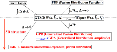
Figure 1: 3D structure functions and Wigner distributions.

The situation is illustrated in Fig. 1. The nucleonic PDFs and form factors have been investigated for a long time, and recent studies focus on the 3D structure functions, GPDs, TMDs, and GDAs. These functions are obtained by integrating the generating functions, generalized transverse-momentum-dependent parton distributions (GTMDs) or Wigner distributions. Although there are much experimental progress on the GPDs and TMDs in the last several years, there was no experimental information on the GDAs until recently. However, the Belle collaboration reported the cross-section data on the two-photon process $\gamma^{*}\gamma\to\pi^{0}\pi^{0}$ in 2016 Masuda:2015yoh , so that it became possible to extract the pion GDAs from their data gdas-kst-2017 .

The determination of the GDAs is valuable in studying 3D tomography of hadrons for finding the origin of nucleon spin, because the GPDs and GDAs are related by the $s$-$t$ crossing and because both distributions are obtained from common double distributions by using the Radon transform as explained in Sect. 2. Such tomography studies could be used also for probing internal structure of exotic hadron candidates because an unstable hadron pair could be produced in the two-photon process gdas-kk-2014 , whereas unstable hadrons cannot be used as fixed targets in measuring the GPDs and TMDs. There is another important advantage in studying the GPDs and GDAs for probing gravitational source by the energy-momentum tensor of quarks and gluons.

The electric charge and magnetic form factors of the nucleons are measured in electron scattering and their radii are determined from them. The charge radius of the pion is measured as $0.672\pm 0.008$ fm. The charged particles in the pion, namely quarks, contribute to the charge form factor and the radius. In the same way, it is interesting to measure the gravitational mass distributions and radii for the pion or any hadron. Here, both quarks and gluons contribute to the gravitational distributions. It is not measured in direct scattering experiment like the electron scattering because of the ultra-weak nature of gravitational interactions. However, there is a way to access them by the 3D structure functions, such as the GDAs, because they contain the factors of the energy-momentum tensor for quarks and gluons gdas-kst-2017 . We know the the energy-momentum tensor is the source of gravity.

We discuss determination of the pion GDAs and gravitational form factors by analyzing the Belle measurements in this report gdas-kst-2017 . First, the GDAs are introduced in Sect. 2, and the cross section of the two-photon process $\gamma^{*}\gamma\to\pi^{0}\pi^{0}$ is explained with the GDAs in Sect. 3. Analysis results are shown in Sect. 4, and our studies are summarized in Sect. 5

2 Generalized distribution amplitudes and gravitational form factors

We explain the GDAs in comparison with the GPDs, which have been studied extensively. First, the GPDs can be experimentally studied by the DVCS $\gamma^{*}h\to\gamma h$ in Fig. 2$(a)$ if $Q^{2}=-q^{2}$ is large enough to satisfy the factorization that the process is described by the hard perturbative QCD part and the soft GPD one. Here, $q$ is the initial virtual-photon momentum. The $s$-$t$ crossed process of the DVCS is the two-photo process to produce a hadron pair $\gamma^{*}\gamma\to h\bar{h}$ as shown in Fig. 2$(b)$. It is also factorized into the hard part and the soft GDA one if $Q^{2}$ is large enough.

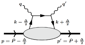
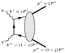
$(a)$                                                 $(b)$

Figure 2:  $(a)$ Virtual Compton process for GPDs           $(b)$ Two-photon process for GDAs.

The pion GPDs $H_{q}^{\,\pi^{0}}$ are defined by off-forward matrix elements of quark and gluon operators with a lightcone separation, and the GDAs $\Phi_{q}^{\,\pi^{0}\pi^{0}}$ are defined by the same operator between the vacuum and the hadron pair as gpds-gdas-rev ; gdas

$$H_{q}^{\,\pi^{0}}(x,\xi,t) =\int\frac{dy^{-}}{4\pi}\,e^{ix\bar{P}^{+}y^{-}}\left<\pi^{0}(p^{\prime})\left|\overline{q}(-y/2)\gamma^{+}q(y/2)\right|\pi^{0}(p)\right>\Big{|}_{y^{+}=\vec{y}_{\perp}=0},$$

$$\Phi_{q}^{\,\pi^{0}\pi^{0}}(z,\zeta,W^{2}) =\int\frac{dy^{-}}{2\pi}\,e^{i(2z-1)\,P^{+}y^{-}/2}\langle\,\pi^{0}(p)\,\pi^{0}(p^{\prime})\,|\,\overline{q}(-y/2)\gamma^{+}q(y/2)\,|\,0\,\rangle\Big{|}_{y^{+}=\vec{y}_{\perp}=0}\,.$$ (1)

These GPDs and GDAs are defined for quarks, and similar expressions exist also for gluons. Here, link operators for the color gauge invariance are not explicitly written for simplicity. The PDFs are given by the forward limit of the GPDs: $q^{\pi^{0}}(x)=H_{q}^{\pi^{0}}(x,\xi=0,t=0)$ for quarks at $x>0$ (antiquark distributions at $x<0$). Using the initial and final pion (photon) momenta $p$ and $p^{\prime}$ ($q$ and $q^{\prime}$), we define average momenta ($\bar{P}$, $\bar{q}$) and momentum transfer $\Delta$ as

$$\bar{P}=\frac{p+p^{\prime}}{2},\ \ \bar{q}=\frac{q+q^{\prime}}{2},\ \ \Delta=p^{\prime}-p=q-q^{\prime}.$$ (2)

Then, the Bjorken variable $x$, the skewdness parameter $\xi$, and the momentum-transfer squared $t$ are given by

$$x=\frac{Q^{2}}{2p\cdot q},\ \ \ \ \xi=\frac{\bar{Q}^{2}}{2\bar{P}\cdot\bar{q}},\ \ \ \ t=\Delta^{2},$$ (3)

where $Q^{2}=-q^{2}$ and $\bar{Q}^{2}=-\bar{q}^{2}$. The DVCS process is factorized, if the kinematical condition $Q^{2}\gg|t|,\ \Lambda_{\text{QCD}}^{2}$ is satisfied, to express it in terms of the GPDs in Fig. 2$(a)$. Here, $\Lambda_{\text{QCD}}$ is the QCD scale parameter.

The variables of the GDAs are the momentum fractions $z$ and $\zeta$ in Fig. 2$(b)$ and the invariant-mass squared $W^{2}$, and they are defined by

$$z=\frac{k\cdot q^{\prime}}{P\cdot q^{\prime}}=\frac{k^{+}}{P^{+}},\ \ \ \zeta=\frac{p\cdot q^{\prime}}{P\cdot q^{\prime}}=\frac{p^{+}}{P^{+}}=\frac{1+\beta\cos\theta}{2},\ \ \ W^{2}=(p+p^{\prime})^{2}=(q+q^{\prime})^{2}=s,$$ (4)

where $\beta$ is the pion velocity given by $\beta=|\vec{p}\,|/p^{0}=\sqrt{1-4m_{\pi}^{2}/W^{2}}$, and the scattering angle is $\theta$ in the center-of-mass frame of final pions. The two-photon process is factorized and expressed by the GDAs if the condition $Q^{2}\gg W^{2},\ \Lambda_{\text{QCD}}^{2}$ is satisfied. The GPDs and GDAs are related with each other by the $s$-$t$ crossing as

$$\Phi_{q}^{\,\pi^{0}\pi^{0}}(z^{\prime},\zeta,W^{2})\longleftrightarrow H_{q}^{\,\pi^{0}}\left(x=\frac{1-2z^{\prime}}{1-2\zeta},\,\xi=\frac{1}{1-2\zeta},\,t=W^{2}\right).$$ (5)

However, the physical regions of the GDAs ($0\leq z\leq 1$, $|1-2\zeta|\leq 1$, $W^{2}\geq 0$) do not necessarily correspond to the physical ones of the GPDs ($|x|\leq 1$, $|\xi|\leq 1$, $t\leq 0$):

$$0\leq|x|<\infty,\ \ 0\leq|\xi|<\infty,\ \ |x|\leq|\xi|,\ \ t\geq 0.$$ (6)

Therefore, the GDA studies may not be directly utilized for clarifying the GPDs. There is a way to circumvent this issue by using the Radon transform, which is often used in tomography studies in general.

Let us consider possible two-pion states in the reaction $\gamma^{*}\gamma\to\pi\pi$. The isospin $I=1$ $\pi\pi$ state is antisymmetric under the exchange of the pions, whereas the $I=0$ and $I=2$ $\pi\pi$ states are symmetric. The $C$ parity of the $\pi\pi$ state is $C=(-1)^{L+S}=(-1)^{L}=1$ with $S=0$ because the $C$ parity of $\gamma^{*}\gamma$ is even. It means $L$ is even. Then, the Pauli principle $(-1)^{L}(-1)^{I}(-1)^{S}=1$ suggests that the $\pi\pi$ isospin state is $I=0$ or 2. However, the GDAs are defined by the vector-type nonlocal operator and the isospin of $\bar{q}q$ is 0 or 1, so that the $\pi\pi$ states from the two photons are $I=0$ with $L=\text{even numbers (0,\,2,\,$\cdots$)}$. Therefore, the GDAs in the process $\gamma^{*}\gamma\to\pi^{0}\pi^{0}$ are $C$-even functions denoted with $(+)$:

$$\Phi_{q}^{\pi^{0}\pi^{0}}(z,\zeta,W^{2})=\Phi^{\pi\pi(I=0)}(z,\zeta,W^{2})=\Phi_{q}^{\pi\pi(+)}(z,\zeta,W^{2}).$$ (7)

The charge-conjugation and isospin symmetries require the relations for the GDAs:

$$\Phi_{q}^{\pi^{0}\pi^{0}}(z,\zeta,W^{2}) =-\Phi_{q}^{\pi^{0}\pi^{0}}(1-z,\zeta,W^{2})=\Phi_{q}^{\pi^{0}\pi^{0}}(z,1-\zeta,W^{2}),$$

$$\Phi_{u}^{\pi^{0}\pi^{0}}(z,\zeta,W^{2}) =\Phi_{d}^{\pi^{0}\pi^{0}}(z,\zeta,W^{2}),$$ (8)

which are considered as constraints in setting up the parametrization of the $\pi^{0}$ GDAs.

The Radon transform is defined for a function $f(x)$ in $n$ dimensions as radon-book

$$\hat{f}(p,\xi)=\int d^{n}x\,f(x)\,\delta(p-\xi\cdot x),$$ (9)

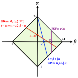
Figure 3: Radon transforms for PDFs, GPDs, and GDAs.

where $x$ is the $n$-dimensional space coordinate [$x$ = ($x_{1}$, $x_{2}$, $\cdots$, $x_{n}$)] and $\xi$ is the unit vector in $n$ dimensions [$\xi$ = ($\xi_{1}$, $\xi_{2}$, $\cdots$, $\xi_{n}$)]. We express the GPDs and GDAs by the common double distributions (DDs) $F_{q}$, $G_{q}$, and $D_{q}$ with different Radon transforms given by teryaev-2001

$$H_{q}(x,\xi,t)=\int d\beta\,d\alpha\,\delta(x-\beta-\xi\alpha)\left[\,F_{q}(\beta,\alpha,t)+\xi G_{q}(\beta,\alpha,t)\,\right],$$

$$\Phi_{q}^{h\bar{h}}(z,\zeta,W^{2})= -2(1-2\zeta)\int d\beta\,d\alpha\delta\big{(}1-2z-(1-2\zeta)\beta+\alpha\big{)}\,$$

$$\ \ \ \ \ \ \ \ \ \ \ \ \ \ \ \times F_{q}(1-2z,\alpha,W^{2})-2D_{q}(x/\xi,W^{2}),$$

$$q(x)= \int_{-1+x}^{1-x}d\alpha\,F_{q}(\beta,\alpha,t=0).$$ (10)

These integral paths are shown in Fig. 3. Namely, the GPDs are obtained by integrating the DDs over the slight line $x=\beta+\xi\alpha$, the PDFs are by the integral over the vertical line with the condition of the forward limit ($t=0$), and the GDAs are by the Radon transform along the different line $1-2z-(1-2\zeta)\beta+\alpha=0$. If the DDs are determined by the GDA studies, they can be used for finding the GPDs and vice verse. Therefore, the GDA studies should be valuable for clarifying the 3D tomography of hadrons and also finding the origin of nucleon spin including orbital-angular-momentum contributions.
There is an important application of the GPD and GDA studies for investigating gravitational aspects of hadrons. The GPDs and GDAs are defined in Eq. (1) with the common nonlocal operator. If the $n$-th moment of this operator is calculated, we obtain

$$\!\!2(P^{+}/2)^{n}\!\!\int_{0}^{1}dz\,(2z-1)^{n-1}\!\!\int\frac{dy^{-}}{2\pi}e^{i(2z-1)P^{+}y^{-}/2}\overline{q}(-y/2)\gamma^{+}q(y/2)\Big{|}_{y^{+}=\vec{y}_{\perp}=0}=\overline{q}(0)\gamma^{+}\!\left(i\overleftrightarrow{\partial}^{+}\right)^{n-1}q(0).$$ (11)

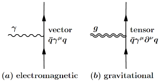
Figure 4: Electromagnetic and gravitational form factors.

We notice in this equation that the right-hand side is the usual vector-type current $\bar{q}\gamma^{\,\mu}q$ for $n=1$ and the second ($n=2$) moment is the energy-momentum tensor $\bar{q}\gamma^{\,\mu}i\partial^{\nu}q$ for quarks as shown in Fig. 4. Actually, the second moment is expressed as gdas

$$\int_{0}^{1}dz\,(2z-1)\,\Phi_{q}^{\pi^{0}\pi^{0}}(z,\,\zeta,\,W^{2})$$

$$\ \ \ \ =\frac{2}{(P^{+})^{2}}\langle\,\pi^{0}(p)\,\pi^{0}(p^{\prime})\,|\,T_{q}^{++}(0)\,|\,0\,\rangle.$$ (12)

In general, the quark energy-momentum tensor is defined by $T_{q}^{\,\mu\nu}(x)=\overline{q}(x)\,\gamma^{\,(\,\mu}i\overleftrightarrow{D}^{\nu)}\,q(x)$, where $D^{\mu}$ is the covariant derivative $D^{\mu}=\partial^{\,\mu}-ig\lambda^{a}A^{a,\mu}/2$ with the QCD coupling constant $g$ and the SU(3) Gell-Mann matrix $\lambda^{a}$.

The matrix element of the energy-momentum tensor is expressed in terms of the timelike gravitational form factors $\Theta_{1}(s)$ and $\Theta_{2}(s)$ as

$$\langle\,\pi^{0}(p)\,\pi^{0}(p^{\prime})\,|\,T_{q}^{\mu\nu}(0)\,|\,0\,\rangle=\frac{1}{2}\left[\,\left(s\,g^{\,\mu\nu}-P^{\,\mu}P^{\nu}\right)\,\Theta_{1,q}(s)+\Delta^{\mu}\Delta^{\nu}\,\Theta_{2,q}(s)\,\right],$$ (13)

where $P=p+p^{\prime}$ and $\Delta=p^{\prime}-p$. Using Eqs. (12) and (13), we can calculate the timelike gravitational form factors $\Theta_{1}(s)$ and $\Theta_{2}(s)$ if the GDAs are determined by analyzing experimental data on $\gamma^{*}\gamma\to\pi^{0}\pi^{0}$. The spacelike gravitational form factors $\Theta_{1}(t)$ and $\Theta_{2}(t)$ are defined by the matrix element as

$$\langle\,\pi^{0}(p^{\prime})\,|\,T_{q}^{\mu\nu}(0)\,|\,\pi^{0}(p)\,\rangle=\frac{1}{2}\left[\,\left(t\,g^{\,\mu\nu}-q^{\,\mu}q^{\nu}\right)\,\Theta_{1,q}(t)+P^{\,\mu}P^{\nu}\,\Theta_{2,q}(t)\,\right],$$ (14)

where $q=p^{\prime}-p$. The spacelike form factors are calculated by using the dispersion relation from the timelike ones, which are obtained directly from the determined GDAs. As explained in Sect. 4, the form factor $\Theta_{2}$ indicates the gravitational mass (energy) distribution and $\Theta_{1}$ is the mechanical (pressure, shear force) distribution.

3 Cross section for two-photon process $\gamma^{*}\gamma\to\pi^{0}\pi^{0}$ and GDAs

We analyze cross-section measurements for the two-photon process $\gamma^{*}\gamma\to\pi^{0}\pi^{0}$ and try to determine the GDAs of the pion. The cross section is expressed by the matrix element ${\cal M}(\gamma^{*}\gamma\to\pi^{0}\pi^{0})$ as

$$d\sigma=\frac{1}{4q\cdot q^{\prime}}\underset{\lambda,\lambda^{\prime}}{\overline{\sum}}|{\cal M}(\gamma^{*}\gamma\to\pi^{0}\pi^{0})|^{2}\,\frac{d^{3}p}{(2\pi)^{3}\,2E_{p}}\frac{d^{3}p^{\prime}}{(2\pi)^{3}\,2E_{p^{\prime}}}(2\pi)^{4}\delta^{4}(q+q^{\prime}-p-p^{\prime}),$$ (15)

and it is written by the hadron tensor ${\cal T}_{\mu\nu}$ and photon-polarization vectors $\epsilon^{\,\mu}(\lambda)$ and $\epsilon^{\nu}(\lambda^{\prime})$ as $i{\cal M}(\gamma^{*}\gamma\to\pi^{0}\pi^{0})=\epsilon^{\mu}(\lambda)\,\epsilon^{\nu}(\lambda^{\prime})\,{\cal T}_{\mu\nu}$. The hadron tensor is generally defined by the matrix element of the electromagnetic current $J_{\mu}^{em}$ and then by the GDAs for the pion, if the hard scale satisfies the factorization condition $Q^{2}\gg W^{2},\ \Lambda_{\text{QCD}}^{2}$, in the leading order of the running coupling constant $\alpha_{s}$ and leading twist gdas-kst-2017 :

$$\!\!\!{\cal T}_{\mu\nu}=i\!\!\int\!d^{4}y\,{e^{-iq\cdot y}}\!\left\langle\pi^{0}(p)\pi^{0}(p^{\prime})\!\left|{TJ_{\mu}^{em}(y)J_{\nu}^{em}(0)}\right|0\right\rangle=-g_{T}^{\,\mu\nu}{e^{2}}\sum\limits_{q}\frac{{e_{q}^{2}}}{2}\!\int_{0}^{1}\!\!{dz}\frac{{2z-1}}{{z(1-z)}}\Phi_{q}^{\pi^{0}\pi^{0}}(z,\zeta,{W^{2}}),$$ (16)

where $g_{T}^{\,\mu\nu}=-1$ for $\mu=\nu=1,\ 2$ and $g_{T}^{\,\mu\nu}=0$ for $\mu$, $\nu=\,$others. The helicity amplitude $A_{ij}$ is defined as $A_{ij}=\varepsilon_{\mu}^{(i)}(q)\,\varepsilon_{\nu}^{(j)}(q^{\prime})\,{{\cal T}^{\mu\nu}}/e^{2}$ ($i=-,\ 0,\ +\,;\ j=-,\ +\,$), and the differential cross section is expressed by the helicity amplitude $A_{++}$:

$$\frac{d\sigma}{d(\cos\theta)}=\frac{\pi\alpha^{2}}{4(Q^{2}+s)}\sqrt{1-\frac{4m_{\pi}^{2}}{s}}\,|A_{++}|^{2},\ \ \ A_{++}=\sum_{q}\frac{e_{q}^{2}}{2}\int^{1}_{0}dz\frac{2z-1}{z(1-z)}\Phi_{q}^{\pi^{0}\pi^{0}}(z,\xi,W^{2}),$$ (17)

where the parity-conservation relation $A_{--}=A_{++}$ is used. The gluon GDA contributes in the higher-order of $\alpha_{s}$, and the terms $A_{0+}$ and $A_{0-}$ are higher-twist ones. They are neglected in our analysis.

Because of the page limitation, the details of the GPD parametrization are not discussed in this article and they should be found in Ref. gdas-kst-2017 . Only the outline is explained in the following. First, the GPDs should satisfy the symmetry relations in Eq. (8). The asymptotic ($Q^{2}\to\infty$) $z$-dependence form is given by $z(1-z)(2z-1)$ for the $\pi^{0}$ GDAs, so that the parameter $\alpha$ may be assigned to its functional form as $z^{\alpha}(1-z)^{\alpha}(2z-1)$. Since there are S- and D-wave contributions to the $\pi^{0}\pi^{0}$ state, the quark GPDs are expressed as

$$\Phi_{q}^{\pi^{0}\pi^{0}}(z,\zeta,W^{2}) =N_{\alpha}z^{\alpha}(1-z)^{\alpha}(2z-1)\,[\widetilde{B}_{10}(W^{2})+\widetilde{B}_{12}(W^{2})P_{2}(\cos\theta)],$$ (18)

where $P_{2}(\cos\theta)$ is the Legendre polynomial. The S- and D-wave terms are $\widetilde{B}_{10}(W^{2})$ and $\widetilde{B}_{12}(W^{2})$, respectively, and they are given by the GDA continuum part and resonance contributions from $f_{0}(500)$ and $f_{2}(1270)$ teryaev-2005-f2 :

$$\widetilde{B}_{10}(W^{2}) =-\bigg{[}\,\left(1+\frac{2\,m_{\pi}^{2}}{W^{2}}\right)\frac{10}{9}M_{2(q)}^{\pi}F^{\,\pi}_{q}(W^{2})+\sum_{f_{0}}\frac{5\,g_{f_{0}\pi\pi}\,\bar{f}_{f_{0}}}{3\sqrt{2}\sqrt{(M^{2}_{f_{0}}-W^{2})^{2}+\Gamma^{2}_{f_{0}}M^{2}_{f_{0}}}}\,\bigg{]}\,e^{i\delta_{0}(W)},$$

$$\widetilde{B}_{12}(W^{2}) =\left(1-\frac{4\,m_{\pi}^{2}}{W^{2}}\right)\frac{10}{9}\,\bigg{[}\,M_{2(q)}^{\pi}F^{\,\pi}_{q}(W^{2})+\frac{g_{f_{2}\pi\pi}\,f_{f_{2}}M^{2}_{f_{2}}\beta^{2}}{\sqrt{2}\sqrt{(M^{2}_{f_{2}}-W^{2})^{2}+\Gamma^{2}_{f_{2}}M^{2}_{f_{2}}}}\,\bigg{]}\,e^{i\delta_{2}(W)}.$$ (19)

The decay constants $\bar{f}_{f_{0}}$ and $f_{f_{2}}$ ($\equiv f_{f}$ ) have $Q^{2}$ dependence, and it is expressed as

$$f_{f}(Q^{2})=f_{f}(Q_{0}^{2})\,\left[\frac{\alpha_{s}(Q^{2})}{\alpha_{s}(Q_{0}^{2})}\right]^{\gamma_{n}/\beta_{0}}\!\!,\ \ \ \ \gamma_{n}=C_{F}\left[\,1-\frac{2}{(n+1)(n+2)}+4\sum_{j=2}^{n+1}\frac{1}{j}\,\right],$$ (20)

effectively by including the scale dependence of the distribution amplitude part gdas-kk-2014 . These decay constants are evaluated by the QCD sum rule often at $Q^{2}=1$ GeV², so that they are evolved to the average scale $\langle Q^{2}\rangle=16.6$ GeV² of the used Belle data. The scale dependence of the decay constants indicates $f_{f}(Q^{2}\to\infty)=0$, which means the resonance contributions vanish in the scaling limit. In this limit, there are sum rules for the GDAs as

$$\int_{0}^{1}dz\,\Phi_{q}^{\,\pi^{0}\pi^{0}}(z,\zeta,W^{2})=0,\ \ \ \ \int_{0}^{1}dz\,(2z-1)\,\Phi_{q}^{\,\pi^{0}\pi^{0}}(z,\zeta,0)=-4\,M_{2(q)}^{\pi^{0}}\,\zeta(1-\zeta).$$ (21)

Here, $M_{2(q)}^{h}$ is the momentum fraction carried by flavor-$q$ quarks and antiquarks in the pion, so that the total quark fraction is $\sum_{q}M_{2(q)}^{\pi^{0}}$. The first terms of $\widetilde{B}_{10}$ and $\widetilde{B}_{12}$ in Eq. (19) are constrained at $W^{2}=0$ by the second sum rule. From Eqs. (12), (13), and (18), we obtain the timelike gravitational form factors expressed by the S- and D-wave terms of the GDAs as

$$\Theta_{1,q}(s)=-\frac{3}{5}\widetilde{B}_{10}(W^{2})+\frac{3}{10}\widetilde{B}_{20}(W^{2}),\ \ \ \Theta_{2,q}(s)=\frac{9}{10\,\beta^{2}}\widetilde{B}_{20}(W^{2}),$$ (22)

and the total timelike gravitational form factors of the pion is obtained by adding them as $\Theta_{n}(s)=\sum_{i=q}\Theta_{n,i}(s)$ where $n=1$ or 2. We notice that the form factor $\Theta_{2}$ originates from the D-wave part of the GDAs and $\Theta_{1}$ from both S- and D-wave terms. The overall form factor for the continuum term is taken as $F^{\,\pi}_{q}(W^{2})=1/[1+(W^{2}-4m_{\pi}^{2})/\Lambda^{2}]^{n-1}$ with the cutoff $\Lambda$ and the factor $n$ taken as the constituent-counting value $n=2$ counting .

The $f_{0}(980)$ contribution is not included in the analysis because the differential cross-section data of the Belle do not show such contribution in the invariant-mass region at $W\simeq 1$ GeV and because there is no theoretical estimate on the decay constant by reflecting its exotic nature, tetra-quark or $K\bar{K}$ configuration. There is a QCD-sum-rule calculation by assuming an ordinary $q\bar{q}$-type configuration for $f_{0}(980)$; however, calculated cross sections are totally in contradiction to the Belle data. It means that the $q\bar{q}$ structure is not supported by the differential cross section data of the Belle collaboration for $f_{0}(980)$ as it has been claimed for a long time f0-4q .

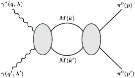
Figure 5: Intermediate-meson contribution.

Some explanations are needed for understanding Eq. (19). First, we comment on coupling constants. There are theoretical estimates on the decay constant $f_{f_{2}}$, and another one $\bar{f}_{f_{0}}$ is considered as a parameter in our analysis because there is no theoretical estimate. The coupling constants $g_{f_{0}\pi\pi}$ and $g_{f_{2}\pi\pi}$ are determined by the $2\pi$ decay widths. Second, there are contributions to the cross section $\gamma^{*}\gamma\to\pi^{0}\pi^{0}$ from the processes with intermediate mesons as shown in Fig. 5. Considering the $\pi\pi$ intermediate state, we need to include the $\pi\pi$ phase shifts $\delta_{0}(W)$ and $\delta_{2}(W)$ in Eq. (19). In our analysis, we use the $\pi\pi$ phase shifts by Bydzovsky, Kaminski, Nazari, and Surovtsev pi-pi-code . Above the $K\bar{K}$ threshold at $2m_{K^{+}}=0.987$ GeV, the $K\bar{K}$ channel opens, and then $\eta\eta$ channel also opens at higher energies. We do not include these effects in our current analysis; however, we introduce additional parameters in the $\pi\pi$ phase shifts above the $K\bar{K}$ threshold and they are determined by fitting the Belle data.

4 Analysis results

The Belle experimental data for $\gamma^{*}\gamma\to\pi^{0}\pi^{0}$ are analyzed for extracting the pion GDAs. For this purpose, we select the data with large enough $Q^{2}$ to satisfy the factorization condition $Q^{2}\gg W^{2},\,\Lambda_{\text{QCD}}^{2}$ so that the amplitude is factorized into the hard perturbative QCD part and the soft GDA one. As such a condition, we take the scale $Q^{2}\geq 8.92$ GeV² for the Belle data. Then, there are 550 points of data with the scales $Q^{2}=$8.92, 10.93, 13.37, 17.23, and 24.25 GeV². The invariant-mass range is $0.5\ \text{GeV}<W<2.1\ \text{GeV}$, and the scattering angles are $\cos\theta=0.1$, 0.3, 0.5, 0.7, and 0.9 in the data.

Figure 6: Comparison with Belle data gdas-kst-2017 .       Figure 7: Timelike gravitational form factors for $\pi$ gdas-kst-2017 .

The pion GDAs are determined by fitting these cross-section data with the equations in the previous section gdas-kst-2017 . The theoretical cross sections are compared with the Belle data, as an example, at $Q^{2}=$8.92, 13.37 GeV² and $\cos\theta=0.1$, 0.5 in Fig. 7. Here, the results are shown by introducing phase parameters for the S-wave phase. We obtained a reasonable result to explain the data. At $\cos\theta=0.1$, there is a conspicuous peak from $f_{2}(1270)$ in the cross section; however, it becomes relatively small at $\cos\theta=0.5$. There is a $f_{0}(500)$ effect at small $W$, and it overlaps with the continuum term in Eq. (19). From the determined GDAs, we calculate the timelike gravitational form factors in Fig. 7 by using Eq. (22). Since they are timelike, they contain both real and imaginary parts. In $\Theta_{2}$, the $f_{2}(1270)$ resonance feature is clear at $\sqrt{s}=1.27$ GeV, whereas $\Theta_{1}$ has more complicated $s$ dependence with both S- and D-wave contributions.

The timelike form factors are converted to the spacelike ones by using the dispersion integral over the real positive $t$ ($\equiv s$) with the consideration that singularities of the form factor $\Theta_{n}(t)$ ($n=1,\,2$) is in the positive real $t$ axis from $4m_{\pi}^{2}$:

$$\Theta_{n}(t) =\int_{4m_{h}^{2}}^{\infty}\frac{ds}{\pi}\frac{{\rm Im}\,\Theta_{n}(s)}{s-t-i\varepsilon}.$$ (23)

Then, the space-coordinate densities are calculated by the Fourier transforms of the spacelike form factors:

$$\rho_{n}(r)=\int\frac{d^{3}q}{(2\pi)^{3}}\,e^{-i\vec{q}\cdot\vec{r}}\,\Theta_{n}(q)=\int_{4m_{h}^{2}}^{\infty}\frac{ds}{4\pi^{2}}\frac{e^{-\sqrt{s}r}}{r}\,{\rm Im}\,\Theta_{n}(s).$$ (24)

Using these equations, we obtain the form factors and densities in Figs. 9 and 9 gdas-kst-2017 .

Physics meaning of these form factors and densities is understood in the following way. The static energy-momentum tensor may be defined by the three-dimensional Fourier transform as static-form $T^{\mu\nu}_{q}(\vec{r}\,)=\int d^{3}q/[(2\pi)^{3}\,2E]e^{i\vec{q}\cdot\vec{r}}\left\langle\pi^{0}(p^{\prime})\!\left|T^{\mu\nu}_{q}(0)\,\right|\!\pi^{0}(p)\right\rangle$ with the pion energy $E=\sqrt{m_{\pi}^{2}+\vec{q}^{\ 2}/4}$. The $\mu\nu=00$ component satisfies the mass relation $\int d^{3}r\,T^{00}_{q}(\vec{r}\,)=m_{\pi}\Theta_{2,q}(0)$, which means that $\Theta_{2}$ and $\rho_{2}(r)$ indicate the mass (energy) distributions in the pion. At finite $t$, $\Theta_{1}$ also contributes to the mass distribution. The $\mu\nu=ij$ ($i,\,j=1,\,2,\,3$) components are generally written as $T^{\,ij}_{q}(\vec{r}\,)=p_{q}(r)\,\delta_{ij}+s_{q}(r)(r_{i}r_{j}/r^{2}-\delta_{ij}/3)$ in terms of the pressure $p(r)$ and shear force $s(r)$. Since $T^{\,ij}_{q}(\vec{r}\,)$ is expressed by only $\Theta_{1}$, $\Theta_{1}$ and $\rho_{1}(r)$ indicate pressure and shear-force distributions in the pion. We may call $\Theta_{2}$ and $\rho_{2}(r)$ the gravitational mass (or energy) form factor and density, and $\Theta_{1}$ and $\rho_{1}(r)$ may be called the mechanical (pressure, shear force) form factor and density. As shown in Figs. 9 and 9, the mass density has a harder distribution than the mechanical one. From the form factors or densities, we obtain the root-mean-square (rms) radii for both distributions: $\sqrt{\langle r^{2}\rangle_{\text{mass}}}=0.69\,\text{fm}$ and $\sqrt{\langle r^{2}\rangle_{\text{mech}}}=1.45\,\text{fm}$. We mentioned that the parameters are introduced for the S-wave phase; however, an equally good fit is also obtained by assigning them to the D-wave part. In the D-wave case, our results are slightly different and there are some ambiguities on this assignment. By considering this ambiguity, we obtain the evaluated gravitational radii as gdas-kst-2017 :

$$\sqrt{\langle r^{2}\rangle_{\text{mass}}}=0.56\sim 0.69\,\text{fm},\ \ \ \sqrt{\langle r^{2}\rangle_{\text{mech}}}=1.45\sim 1.56\,\text{fm}.$$ (25)

This is the first report on the gravitational radii for a hadron from experimental measurements. It is especially interesting to find that the mass radius is similar or slightly smaller than the charge radius $\sqrt{\langle r^{2}\rangle_{\text{charge}}}=0.672\pm 0.008$ fm and that the mechanical radius is larger. However, the studies of the gravitational form factors and radii for hadrons are still in the beginning stage, and further investigations are needed.

Figure 8: Spacelike gravitational form factors gdas-kst-2017 .       Figure 9: Mass and mechanical densities gdas-kst-2017 .

We believe that this new field has bright future to understand gravitational physics from microscopic quark and gluon level. Gravity studies are mainly on macroscopic systems because gravitational interactions are ultra-weak ones and they cannot be detected generally in microscopic particle-physics measurements. However, as we explained in this report, we can find the gravitational source originates from quarks and gluons by using the technique of hadron tomography, namely by the 3D structure functions. The KEKB will produce much accurate cross-section data in the near future by the upgraded super-KEKB, so that the errors in Fig. 7 should become much smaller in a few years. Furthermore, the 3D structure functions can be investigated at various high-energy facilities in the world such as LHC, RHIC, CERN-COMPASS, JLab, Fermilab, J-PARC, GSI, and ILC. Time has come to investigate the 3D tomography including the GDAs for clarifying gravitational properties of hadrons.

5 Summary

We have determined the GDAs, gravitational form factors, and densities for the pion by analyzing the Belle cross-section measurements on the two-photon process $\gamma^{*}\gamma\to\pi^{0}\pi^{0}$. The GDAs are provided with several parameters by considering the continuum term and resonances ones, and they are determined from the Belle data. By taking the first moments of the GDAs, we obtained the timelike gravitational form factors ($\Theta_{1}$, $\Theta_{2}$) for the pion. Using the dispersion relation, they are converted to the spacelike form factors. Then, the space-coordinate distributions ($\rho_{1}(r)$, $\rho_{2}(r)$) and rms radii, $\sqrt{\langle r^{2}\rangle_{\text{mass}}}=0.56\sim 0.69$ fm and $\sqrt{\langle r^{2}\rangle_{\text{mech}}}=1.45\sim 1.56$ fm, are calculated. The functions $\Theta_{2}$ and $\rho_{2}(r)$ have the meaning of the gravitational mass (energy) form factor and density, and $\Theta_{1}$ and $\rho_{1}(r)$ are the mechanical (pressure, shear force) form factor and density. This should be the first finding on the gravitational form factors and radii for a hadron by analyzing actual experimental measurements. The charge radius of the pion is $0.672\pm 0.008$ fm. It is our interesting finding that the gravitational mass radius is similar to this charge radius or slightly smaller, and the mechanical radius is larger.

Since the 3D tomography has been a very popular topic in hadron physics in the last several years, much progress is expected in this novel field of gravitational physics from the fundamental quark and gluon level. Gravitational physics in microscopic systems had been a speculative project for a long time due to ultra-weak interaction nature. However, time has come to investigate it in the microscopic level because the gravitational source from quarks and gluons can be determined, as we showed in this work. Our work is just the beginning of such studies, and much progress is expected in this new research area.

References

- (1) M. Masuda et al. (Belle Collaboration), Phys. Rev. D 93, 032003 (2016).
- (2) S. Kumano, Qin-Tao Song, and O. V. Teryaev, arXiv:1711.08088 [hep-ph].
- (3) H. Kawamura and S. Kumano, Phys. Rev. D 89, 054007 (2014).
- (4) For a review, see M. Diehl, Phys. Rept. 388, 41 (2003).
- (5) M. Diehl, T. Gousset, B. Pire, and O. Teryaev, Phys. Rev. Lett. 81, 1782 (1998); M. Diehl, T. Gousset, and B. Pire, Phys. Rev. D 62, 073014 (2000); M. V. Polyakov, Nucl. Phys. B 555, 231 (1999); M. V. Polyakov and C. Weiss, Phys. Rev. D 60, 114017 (1999).
- (6) S. R. Deans, The Radon transform and some of its applications, (Dover Publications Ins., Mineola, New York, 1992).
- (7) O. V. Teryaev, Phys. Lett. B 510, 125 (2001); C. Mezrag, H. Moutarde, and J. Rodriguez-Quintero, Few Body Syst. 57, 729 (2016).
- (8) I. V. Anikin, B. Pire, L. Szymanowski, O. V. Teryaev, and S. Wallon, Phys. Rev. D 71, 034021 (2005).
- (9) H. Kawamura, S. Kumano, and T. Sekihara, Phys. Rev. D 88, 034010 (2013). W.-C. Chang, S. Kumano, and T. Sekihara, Phys. Rev. D 93, 034006 (2016).
- (10) S. Kumano, V. R. Pandharipande, Phys. Rev. D 38, 146 (1988); F. E. Close, N. Isgur, and S. Kumano, Nucl. Phys. B 389, 513 (1993); T. Sekihara and S. Kumano, Phys. Rev. D 92, 034010 (2015).
- (11) V. Nazari, P. Bydzovsky, and R. Kaminski, Phys. Rev. D 94, 116013 (2016); P. Bydzovsky, R. Kaminski, and V. Nazari, Phys. Rev. D 90, 116005 (2014).
- (12) M. V. Polyakov, Phys. Lett. B 555, 57 (2003).