Local Causal States
and
Discrete Coherent Structures

Local Causal States
and
Discrete Coherent Structures

Abstract

Coherent structures form spontaneously in nonlinear spatiotemporal systems and are found at all spatial scales in natural phenomena from laboratory hydrodynamic flows and chemical reactions to ocean, atmosphere, and planetary climate dynamics. Phenomenologically, they appear as key components that organize the macroscopic behaviors in such systems. Despite a century of effort, they have eluded rigorous analysis and empirical prediction, with progress being made only recently. As a step in this, we present a formal theory of coherent structures in fully-discrete dynamical field theories. It builds on the notion of structure introduced by computational mechanics, generalizing it to a local spatiotemporal setting. The analysis’ main tool employs the local causal states, which are used to uncover a system’s hidden spatiotemporal symmetries and which identify coherent structures as spatially-localized deviations from those symmetries. The approach is behavior-driven in the sense that it does not rely on directly analyzing spatiotemporal equations of motion, rather it considers only the spatiotemporal fields a system generates. As such, it offers an unsupervised approach to discover and describe coherent structures. We illustrate the approach by analyzing coherent structures generated by elementary cellular automata, comparing the results with an earlier, dynamic-invariant-set approach that decomposes fields into domains, particles, and particle interactions.

Patterns abound in systems far from equilibrium across all spatial scales, from planetary and even galactic structures down to the microscopic scales of snowflakes and bacterial and crystal growth. Most studies of pattern formation, both theory and experiment, focus on particular classes of human-scale pattern-forming system and invoke standard bases to describe pattern organization. This becomes particularly problematic when, for example, inhomogeneities give rise to relatively more localized patterns, called coherent structures. Though key to structuring a system’s macroscopic behaviors and causal organization, they have remained elusive for decades. We suggest an alternative approach that provides constructive answers to the questions of how to use spacetime fields generated by spatiotemporal systems to extract their emergent patterns and how to describe them in an objective way.

I Introduction

Complex patterns are generated by systems in which interactions among their basic elements are amplified, propagated, and stabilized in a complicated manner. These emergent patterns present serious difficulties for traditional mathematical analysis, as one does not know a priori in what representational basis to describe them, let alone predict them. Notably, analogous difficulties of describing and predicting the behavior of highly complex systems had been identified in the early years of computation theory [1] and linguistics [2].

A more familiar and perhaps longer-lived example of complex emergent patterns arises in fluid turbulence [3]. From its earliest systematic studies, complex flow patterns were described as linear combinations of periodic solutions. The maturation of nonlinear dynamical systems theory, though, led to a radically different view: The mechanism generating complex, unpredictable behavior was a relatively low-dimensional strange attractor [4, 5, 6]. Using behavior-driven “state-space reconstruction” techniques [7, 8] this hypothesis was finally demonstrated [9]. The behavior-driven methods were even extended to extracting the equations of motion themselves from time series of observations [10]. Success in this required knowing an appropriate language with which to express the equations of motion. Those successes, however, tantalizingly suggested that behavior-driven methods could let a system’s behavior determine the basis for identifying and describing their emergent patterns.

To lay the foundations for this and determine what was required for success, a new approach to discovering patterns generated by complex systems—computational mechanics [11, 12, 13]—was developed. It employs mathematical structures analogous to those found in computation theory to build intrinsic representations of temporal behavior. The structure of a system’s dynamic, the rules of its temporal evolution, are captured and quantified by the intrinsic representations of computational mechanics—its $\epsilon$-machines. Before this view was introduced, one was tempted to assume a system’s evolution rules were simply its equations of motion. A hallmark of emergent systems, however, arises exactly when this is not the case [14]. While a system’s emergent dynamical structure ultimately derives from the governing equations of motion, arriving at the former from the latter is typically unfeasible. Similarly, chemistry cannot be considered simply as “applied physics” nor biology, “applied chemistry” [15].

The use of automata-theoretic constructs lends computational mechanics its name: it extends statistical mechanics beyond statistics to include computation-theoretic mechanisms. Operationally, the rise of computer simulation and numerical analysis as the “third paradigm” for physical sciences provides a research ecosystem that is well-complemented by computational mechanics, as the latter is a theory built to describe behavior (data) and, in this, it focuses relatively less on analyzing governing equations [16]. The need for behavior-driven theory—“data-driven”, as some say today—such as computational mechanics becomes especially apparent in high-dimensional, nonlinear systems.

Patterns abound in systems far from equilibrium across all spatial scales [17, 18, 19], from galactic structures to planetary—such as Jupiter’s famous Red Spot and similar climatological structures on Earth—down to the microscopic scales of snowflakes [20] and bacterial [21] and crystal growth [22]. For imminently practical reasons, though, most studies of pattern formation, both theory [23, 24] and experiment, focus on particular classes of human-scale pattern-forming system, including Rayleigh-Bénard convection [25, 26, 27], Taylor-Couette flow [28, 29], the Belousov-Zhabotinsky chemical reaction [30, 31], and Faraday’s crispations [32, 33] to mention several. Often studied under the rubric of nonequilibrium phase transitions [34, 35, 36], these systems are amenable to careful experimental control and systematic mathematical analysis, facilitated by imposing idealized boundary conditions. Nonequilibrium is maintained in these systems via homogeneous fluxes that give rise to cellular patterns described and analyzed through global Fourier modes.

While much progress has been made in understanding the instability mechanisms driving pattern formation and the dynamics of the patterns themselves in idealized systems [37, 24, 23, 38], many challenges remain, especially with wider classes of real world patterns. In particular, the inescapable inhomogeneities of systems found in nature give rise to relatively more localized patterns, rather than the cellular patterns captured by simple Fourier modes. We refer to these localized patterns as coherent structures. There has been intense interest recently in coherent structures in fluid flows, including structures in geophysical flows [39, 40], such as hurricanes [41, 42], and in more general turbulent flows [43].

A principled universal description of the organization of such structures does not exist. So, while we can exploit vast computing resources to simulate models of ever-increasing mathematical sophistication, analyzing and extracting insights from such simulations becomes highly nontrivial. Indeed, given the size and power of modern computers, analyzing their vast simulation outputs can be as daunting as analyzing any real physical experiment [16]. Finally, there is no unique, agreed-upon approach to analyzing and predicting coherent material structures in fluid flows, for instance [44]. Even today ad hoc thresholding is often used to identify extreme weather events in climate data, such as cyclones and atmospheric rivers [45, 46, 47]. Developing a principled, but general mathematical description of coherent structures is our focus.

Parallels with contemporary machine learning are worth noting, given the increasing overlap between these technologies and the needs of the physical sciences. Imposing Fourier modes as templates for cellular patterns is the mathematical analog of the technology of (supervised) pattern recognition [48]. Patterns are given as a finite number of classes and learning algorithms are trained to assign inputs into these classes by being fed a large number of labeled training data, which are inputs already assigned to the correct pattern class.

Computational mechanics, in contrast, makes far fewer structural assumptions [13]. As we will see, for discrete spatially extended systems it makes only modest yet reasonable assumptions about the existence and conditional stationarity of lightcones in the orbit space of the system. In so doing, it facilitates identifying representations that are intrinsic to a particular system. This is in contrast with subjectively imposing a descriptional basis, such as Fourier modes, wavelets, or engineered pattern-class labels. We say that our subject here is not simply pattern recognition, but (unsupervised) pattern discovery.

To start to address these challenges, we briefly review a particular spatiotemporal generalization of computational mechanics [49]. We adapt it to detect coherent structures in terms of the underlying constituents from which they emerge, while at the same time providing a principled description of such structures. The development is organized as follows. Section II introduces the local causal states, the main tool of computational mechanics used for coherent structure analysis. We also give an overview of elementary cellular automata (ECAs), which is the class of pattern-forming mathematical models we use to demonstrate our coherent structure analysis.

Section III introduces the computational mechanics of coherent structures. The dynamical notion of background domains plays a central role since, after transients die away, the fields produced by spatially extended dynamical systems can be decomposed into domain regions and coherent structures embedded in them [50]. Furthermore, the domains’ internal symmetries typically dictate how the overall spatiotemporal dynamic organizes itself, including what large-scale patterns may form. More to the point, we formally define coherent structures with respect to a system’s domains.

Crutchfield and Hanson introduced a principled analysis of CA domains and coherent structures [11, 50, 51, 52, 53, 54, 55]. They defined domains as dynamically invariant sets of spatially statistically stationary configurations with finite memory. This led to formal methods for proving that domains were spacetime shift-invariant and so dominant patterns for a given CA. Having identified these significant patterns, they created spatial transducers that decomposed a CA spacetime field into domains and nondomain structures, such as particles and particle interactions [56]. We refer to this analysis of CA structures as the domain-particle-interaction decomposition (DPID). The following extends DPID but, for the first time, uses local causal states to define domains and coherent structures. In this, domains are given by spacetime regions where the associated local causal states have time and space translation symmetries.

Section IV gives detailed examples for the two main classes of CA domains—those with explicit symmetries and those with hidden symmetries. We show empirically that there is a strong correspondence between domains and structures of elementary CAs identified by local causal states and by the DPID approach. For domains, we show that a homogeneous invariant set of spatial configurations (DPID domains) produces a local causal state field with a spacetime symmetry tiling. Since local causal state inference is fully behavior-driven, it applies to a broader class of spatiotemporal systems than the DPID transducers. And so, this correspondence extends both the theory and application of the coherent structure analysis they engender.

Similar approaches using local causal states have been pursued by others [57, 58, 59, 60, 61]. However, as will be elaborated upon in future work, these underutilize computational mechanics, developing only a qualitative filtering tool—local statistical complexity—that assists in subjective visual recognition of coherent structures. Moreover, they provide no principled way to describe structures and thus cannot, to take one example, distinguish two distinct types of structures from one another. There have also been other unsupervised approaches to coherent structure discovery in cellular automata using information-theoretic measures [62, 63, 64, 65]. Recent critiques of employing such measures to determine information storage and flow and causal dependency [66, 67] indicate that these uses of information theory for CAs are still in early development and have some distance to go to reach the structure-detection performance levels presented here.

II Background

Modern physics evolved to use group theory to formalize the concept of symmetry [68]. The successes in doing so are legion in twentieth-century fundamental physics. When applied to emergent patterns, though, group-theoretic descriptions formally describe only their exact symmetries. This is too restrictive for more general notions—naturally occurring patterns and structures that are an amalgam of strict symmetry and randomness. Thus, one appeals to semigroup theory [69, 70] to describe partial symmetries. This use of semigroup algebra is fundamental to automata as developed in early computation theory [71, 72]. In this, different classes of automata or “machines” formalize the concept of structure [1]. Through the connection with semigroup theory, structure captured by machines can be seen as a system’s generalized symmetries. The variety of computational model classes [73] then becomes an inspiration for understanding emergent natural patterns [71].

To capture structure in complex physical systems, though, computational mechanics had to move beyond computation-theoretic automata to probabilistic representations of behavior. That said, its parallels to semigroups and automata are outlined in Ref. [12, Apps. D and H], for example. Early on, the theory was most thoroughly developed in the temporal setting to analyze structured stochastic processes . It was also applied to continuous-valued chaotic systems using the methods [75] of symbolic dynamics to partition low-dimensional attractors [11]. More recently, it has been directly applied to continuous-time and continuous-value processes [76, 77, 78, 79, 80, 81, 82].

II.1 Temporal processes, canonical representations

A stochastic process $\mathcal{P}$ is the distribution of all a system’s allowed behaviors or realizations $\ldots{x}_{-2},{x}_{-1},{x}_{0},{x}_{1},\ldots$ as specified by their joint probabilities $\Pr(\ldots,{X}_{-2},{X}_{-1},{X}_{0},{X}_{1},...)$. Here, ${X}_{t}$ is the random variable for the outcome of the measurement ${x}_{t}\in\mathcal{A}$ at time $t$, taking values from a finite set $\mathcal{A}$ of all possible events. (Uppercase denotes a random variable; lowercase its value.) We denote a contiguous chain of $\ell$ random variables as ${X}_{0:\ell}={X}_{0}{X}_{1}\dotsm{X}_{\ell-1}$ and their realizations as ${x}_{0:\ell}={x}_{0}{x}_{1}\dotsm{x}_{\ell-1}$. (Left indices are inclusive; right, exclusive.) We suppress indices that are infinite. We will often work with stationary processes for which $\Pr\big{(}{X}_{t:t+\ell}\big{)}=\Pr\big{(}{X}_{0:\ell}\big{)}$ for all $t$ and $\ell$.

The canonical representation for a stochastic process within computational mechanics is the process’ $\epsilon$-machine. This is a type of stochastic state machine, commonly known as a hidden Markov model (HMM), that consists of a set $\bm{\Xi}$ of causal states and transitions between them. The causal states are constructed for a given process by calculating the classes determined by the causal equivalence relation:

$${x}_{:t}\;{\sim}_{\epsilon}\;{x}_{:t}^{\prime}\iff\Pr({X}_{t:}|{X}_{:t}={x}_{:t})=\Pr({X}_{t:}|{X}_{:t}={x}_{:t}^{\prime})~{}.$$

Operationally, two pasts ${x}_{:t}$ and ${x}_{:t}^{\prime}$ are causally equivalent, i.e., belong to the same causal state, if and only if they make the same prediction for the future. Equivalent states lead to the same future conditional distribution. Behaviorally, the interpretation is that whenever a process generates the same future (a conditional distribution), it is effectively in the same state.

Each causal state $\xi\in\bm{\Xi}$ is an element of the coarsest partition of a process’ pasts $\{{x}_{:t}:t\in\mathbb{Z}\}$ such that every ${x}_{:t}\in\xi$ has the same predictive distribution: $\Pr({X}_{t:}|{x}_{:t})=\Pr({X}_{0:}|\cdot)$. The associated random variable is $\Xi$. The $\epsilon$-function $\epsilon({x}_{:t})$ maps a past to its causal state: $\epsilon:{x}_{:t}\mapsto\xi$. In this way, it generates the partition defined by the causal equivalence relation ${\sim}_{\epsilon}$. One can show that the causal states are the unique minimal sufficient statistic of the past when predicting the future. Notably, the causal state set $\bm{\Xi}$ can be finite, countable, or uncountable [14, 83, 84], even if the original process is stationary, ergodic, and generated by an HMM with a finite set of states. Reference [12] gives a detailed exposition and Refs. [85, 81, 82] give closed-form calculational tools.

II.2 Spatiotemporal processes, local causal states

The state ${x}$ of a spatiotemporal system specifies the values ${x}^{r}$ at sites $r$ of a lattice $\mathcal{L}$. Assuming values lie in set $\mathcal{A}$, a configuration ${x}\in\mathcal{A}^{\mathcal{L}}$ is the collection of values over the lattice sites. If the values are generated by random variables ${X}^{r}$, then we have a spatial process $\Pr({X})$—a stochastic process over the random variable field ${X}=\{{X}^{r}:r\in\mathcal{L}\}$.

A spatiotemporal system, in contrast to a purely temporal one, generates a process $\Pr(\ldots,{X}_{-1},{X}_{0},{X}_{1},\ldots)$ consisting of the series of fields ${X}_{t}$. (Subscripts denote time; superscripts sites.) A realization of a spatiotemporal process is known as spacetime field $\mathbf{{x}}\in\mathcal{A}^{\mathcal{L}\otimes\mathbb{Z}}$, consisting of a time series ${x}_{0},{x}_{1},\ldots$ of spatial configurations ${x}_{t}\in\mathcal{A}^{\mathcal{L}}$. $\mathcal{A}^{\mathcal{L}\otimes\mathbb{Z}}$ is the orbit space of the process; that is, time is added onto the system’s state space. The associated spacetime field random variable is $\mathbf{{X}}$. A spacetime point $\mathbf{{x}}_{t}^{r}\in\mathcal{A}$ is the value of the spacetime field at coordinates $(r,t)$—that is, at location $r\in\mathcal{L}$ at time $t$. The associated random variable at that point is $\mathbf{{X}}_{t}^{r}$.

Being interested in spatiotemporal systems that exhibit spatial translation symmetries, we narrow consideration to regular spatial lattices with topology $\mathcal{L}=\mathbb{Z}^{d}$. (As needed, the lattice will be infinite or periodic along each dimension.)

Purely temporal computational mechanics views the spatiotemporal process $\Pr(\ldots,{X}_{-1},{X}_{0},{X}_{1},\ldots)$ as a time series over events with the very large or even infinite alphabet—the configurations in $\mathcal{A}^{\mathcal{L}}$. In special cases, one can calculate the temporal causal equivalence classes and their causal states and transitions from the time series of spatial configurations, giving the global $\epsilon$-machine. While formally well defined, determining the global $\epsilon$-machine is for all practical purposes intractable. Some form of simplification is required to make headway.

II.2.1 Random variable lightcones

To circumvent this we introduce a different, spatially local representation. This respects and leverages the configurations’ spatial nature; the otherwise unwieldy configuration alphabet $\mathcal{A}^{\mathcal{L}}$ has embedded structure. In particular, for systems that evolve under a homogeneous local dynamic and for which information propagates through the system at a finite speed, it is quite natural to use lightcones as spatially local notions of pasts and futures.

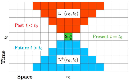
Figure 1: Lightcone random variable templates: Past lightcone $\mathtt{L}^{-}(r_{0},t_{0})$ and future lightcone $\mathtt{L}^{+}(r_{0},t_{0})$ for present spacetime point $\mathbf{{X}}_{t_{0}}^{r_{0}}$ in a $1+1$ D field with nearest-neighbor (or radius-$1$) interactions.

Formally, the past lightcone $\mathtt{L}^{-}$ of a spacetime random variable $\mathbf{{X}}_{t}^{r}$ is the set of all random variables at previous times that could possibly influence it. That is:

$$\mathtt{L}^{-}(r,t)\equiv\big{\{}\mathbf{{X}}_{t^{\prime}}^{r^{\prime}}:\;t^{\prime}\leq t\;\mathrm{and}\;||r^{\prime}-r||\leq c(t^{\prime}-t)\big{\}}~{},$$ (1)

where $c$ is the finite speed of information propagation in the system. Similarly, the future lightcone $\mathtt{L}^{+}$ is given as all the random variables at subsequent times that could possibly be influenced by $\mathbf{{X}}_{t}^{r}$:

$$\mathtt{L}^{+}(r,t)\equiv\big{\{}\mathbf{{X}}_{t^{\prime}}^{r^{\prime}}:\;t^{\prime}>t\;\mathrm{and}\;||r^{\prime}-r||\leq c(t-t^{\prime})\big{\}}~{}.$$ (2)

We include the present random variable $\mathbf{{X}}_{t}^{r}$ in its past lightcone, but not its future lightcone. An illustration for one-space and time ($1+1$D) fields on a lattice with nearest-neighbor (or radius-$1$) interactions is shown in Fig 1. We use $\mathtt{L}^{-}$ to denote the random variable for past lightcones with realizations $\ell^{-}$; similarly, $\mathtt{L}^{+}$ those with realizations $\ell^{+}$ for future lightcones.

The choice of lightcone representations for both local pasts and futures is ultimately a weak-causality argument: influence and information propagate locally through a spacetime site from its past lightcone to its future lightcone. A sequel [86] goes into more depth, exploring this choice and possible variations. For now, we work with the given assumptions.

Using lightcones as local pasts and futures, generalizing the causal equivalence relation to spacetime is now straightforward. Two past lightcones are causally equivalent if they have the same distribution over future lightcones:

$$\ell^{-}_{i}\;{\sim}_{\epsilon}\;\ell^{-}_{j}\iff\Pr\big{(}\mathtt{L}^{+}|\ell^{-}_{i}\big{)}=\Pr\big{(}\mathtt{L}^{+}|\ell^{-}_{j}\big{)}~{}.$$ (3)

This local causal equivalence relation over lightcones implements an intuitive notion of optimal local prediction [49]. At some point $\mathbf{{x}}_{t}^{r}$ in spacetime, given knowledge of all past spacetime points that could possibly affect $\mathbf{{x}}_{t}^{r}$—i.e., its past lightcone $\ell^{-}(r,t)$—what might happen at all subsequent spacetime points that could be affected by $\mathbf{{x}}_{t}^{r}$—i.e., its future lightcone $\ell^{+}(r,t)$?

The equivalence relation induces a set $\bm{\Xi}$ of local causal states $\xi$. A functional version of the equivalence relation is helpful, as in the pure temporal setting, as it directly maps a given past lightcone $\ell^{-}$ to the equivalence class $[\ell^{-}]$ of which it is a member:

$$\epsilon(\ell^{-}) =[\ell^{-}]$$

$$=\{\ell^{-^{\prime}}:\ell^{-}\sim_{\epsilon}\ell^{-^{\prime}}\}$$

or, even more directly, to the associated local causal state:

$$\epsilon(\ell^{-})=\xi_{\ell^{-}}~{}.$$

Closely tracking the standard development of temporal computational mechanics [12], a set of results for spatiotemporal processes parallels those of temporal causal states [49]. For example, one concludes that local causal states are minimal sufficient statistics for optimal local prediction. Moreover, the particular local prediction uses lightcone-shaped random-variable templates, associated with local causality in the system. Specifically, the future follows the past and information propagates at a finite speed. Thus, local causal states do not detect direct causal relationships—say, as reflected in learning equations of motion from data. Rather, they exploit an intrinsic causality in the system in order to discover emergent spacetime structures.

As an aside, if viewed as a form of data-driven machine learning, our coherent-structure theory, implemented using either DPID or local causal states, allows for unsupervised image-segmentation labeling of spatiotemporal structures. We should emphasize that this is spacetime segmentation and not a general image segmentation algorithm [48], since it works only in systems for which local causality exists and for which lightcone templates are well defined.

II.2.2 Causal state filtering

As in purely-temporal computational mechanics, the local causal equivalence relation Eq. (3) induces a partition over the space of (infinite) past lightcones, with the local causal states being the equivalence classes. We will use the same notation for local causal states as was used for temporal causal states above, as there will be no overlap later: $\bm{\Xi}$ is the set of local causal states defined by the local causal equivalence partition, $\Xi$ denotes the random variable for a local causal state, and $\xi$ for a specific realized causal state. The local $\epsilon$-function $\epsilon(\ell^{-})$ maps past lightcones to their local causal states $\epsilon:\ell^{-}\mapsto\xi$, based on their conditional distribution over future lightcones.

For spatiotemporal systems, a first step to discover emergent patterns applies the local $\epsilon$-function to an entire spacetime field to produce an associated local causal state field $\mathcal{S}=\epsilon(\mathbf{{x}})$. Each point in the local causal state field is a local causal state $\mathcal{S}_{t}^{r}=\xi\in\bm{\Xi}$.

The central strategy here is to extract a spatiotemporal process’ pattern and structure from the local causal state field. The transformation $\mathcal{S}=\epsilon(\mathbf{{x}})$ of a particular spacetime field realization $\mathbf{{x}}$ is known as causal state filtering and is implemented as follows. For every spacetime coordinate $(r,t)$:

1. At $\mathbf{{x}}_{t}^{r}$ determine its past lightcone $\mathtt{L}^{-}(r,t)=\ell^{-}$;

2. Form its local predictive distribution $\Pr(\mathtt{L}^{+}|\ell^{-})$;

3. Determine the unique local causal state $\xi\in\bm{\Xi}$ to which it leads; and

4. Label the local causal state field at point $(r,t)$ with $\xi$: $\mathcal{S}_{t}^{r}=\xi$.

Notice the values assigned to $\mathcal{S}$ in step 4 are simply the labels for the corresponding local causal states. Thus, the local causal state field is a semantic field, as its values are not measures of any quantity, but rather labels for equivalence classes of local dynamical behaviors as in the measurement semantics introduced in Ref. [87].

In practice, there are inference details involved in causal filtering which we discuss more in Ref. [86]. The main inference parameters are the finite lightcone horizons $h^{-}$ and $h^{+}$, as well as the speed of information propagation $c$. For cellular automata $c$ is simply the radius $R$ of local neighborhoods; see below. These parameters determine the shape of the lightcone templates that are extracted from spacetime fields.

Causal state filtering will be used shortly in Sec. III to analyze spacetime domains and coherent structures. For each case we will give the past and future lightcone horizons used. But first we must introduce prototype spatial dynamical systems to study.

II.3 Cellular automata

The spatiotemporal processes whose structure we will analyze are deterministically generated by cellular automata. A cellular automaton (CA) is a a fully-discrete spatially-extended dynamical system with a regular spatial lattice in $d$ dimensions $\mathcal{L}=\mathbb{Z}^{d}$, consisting of local variables taking values from a discrete alphabet $\mathcal{A}$ and evolving in discrete time steps according to a local dynamic $\phi$. Time evolution of the value at a site on a CA’s lattice depends only on values at sites within a given radius $R$. The collection of all sites within radius $R$ of a point $\mathbf{{x}}_{t}^{r}$, including $\mathbf{{x}}_{t}^{r}$ itself, is known as the point’s neighborhood $\eta(\mathbf{{x}}_{t}^{r})$:

$$\eta(\mathbf{{x}}_{t}^{r})=\{\mathbf{{x}}_{t}^{r^{\prime}}\;:\;||r-r^{\prime}||\leq R,r,r^{\prime}\in\mathcal{L}\}~{}.$$

The neighborhood specification depends on the form of the lattice distance metric chosen. The two most common neighborhoods for regular lattice configurations are the Moore and von Neumann neighborhoods, defined by the Chebyshev and Manhattan distances in $\mathcal{L}$, respectively.

The local evolution of a spacetime point is given by:

$$\mathbf{{x}}_{t+1}^{r}=\phi\big{(}\eta(\mathbf{{x}}_{t}^{r})\big{)}~{},$$

and the global evolution $\Phi:\mathcal{A}^{\mathcal{L}}\rightarrow\mathcal{A}^{\mathcal{L}}$ of the spatial field is given by:

$$\mathbf{{x}}_{t+1}=\Phi(\mathbf{{x}}_{t})~{}.$$ (4)

For example, this might apply $\phi$ in parallel, simultaneously to all neighborhoods on the lattice. Although, other local update schemes are encountered.

As noted, CAs are fully discrete dynamical systems. They evolve an initial spatial configuration ${x}_{0}\in\mathcal{A}^{\mathcal{L}}$ according to Eq. (4)’s dynamic. This generates an orbit $\mathbf{{x}}_{0:t}=\{\mathbf{{x}}_{0},\mathbf{{x}}_{1},\ldots\mathbf{{x}}_{t-1}\}\in\mathcal{A}^{\mathcal{L}\otimes\mathbb{Z}}$. Usefully, dynamical systems theory classifies a number of orbit types. Most basically, a periodic orbit repeats in time:

$$\mathbf{{x}}_{t+p} =\Phi^{p}(\mathbf{{x}}_{t})$$

$$=\mathbf{{x}}_{t}~{},$$ (5)

where $p$ is its period—the smallest integer for which this holds. A fixed point has $p=1$ and a limit cycle has finite $p>1$. An aperiodic orbit has no finite $p$; a behavior that can occur only on infinite lattices.

Since CA states are spatial configurations an orbit $\mathbf{{x}}_{0:t}$ is a spacetime field. These orbits constitute the spatiotemporal processes of interest in the following.

II.4 Elementary CAs

The prototype spatial systems we use to demonstrate coherent structure analysis are the elementary cellular automata (ECAs) that have a one-dimensional spatial lattice $\mathcal{L}=\mathbb{Z}$ and local random variables taking binary values $\mathcal{A}=\{0,1\}$. Thus, ECA spatial configurations $\mathbf{{x}}_{t}\in\mathcal{A}^{\mathbb{Z}}$ are strings of 0s and 1s. Equation (4)’s time evolution is implemented by simultaneously applying the local dynamic (or lookup table) $\phi$ over radius-$1$ neighborhoods $\eta(\mathbf{{x}}_{t}^{r})=\mathbf{{x}}_{t}^{r-1}\mathbf{{x}}_{t}^{r}\mathbf{{x}}_{t}^{r+1}$:

111O7110O6101O5100O4011O3010O2001O1000O0,fragments 111fragmentsO7110fragmentsO6101fragmentsO5100fragmentsO4011fragmentsO3010fragmentsO2001fragmentsO1000fragmentsO0\displaystyle\begin{tabular}[]{c c c | c}\lx@intercol\hfil$\eta$\hfil\lx@intercol\vrule\lx@intercol &$O_{\eta}=\phi(\eta)$\\ \hline\cr 1&1&1&$O_{7}$\\ 1&1&0&$O_{6}$\\ 1&0&1&$O_{5}$\\ 1&0&0&$O_{4}$\\ 0&1&1&$O_{3}$\\ 0&1&0&$O_{2}$\\ 0&0&1&$O_{1}$\\ 0&0&0&$O_{0}$\end{tabular}~{},

η=Oηϕ(η)η=Oηϕ(η)

where each output $O_{\eta}=\phi(\eta)\in\mathcal{A}$ and the $\eta$s are listed in lexicographical order. There are $2^{8}=256$ possible lookup tables, as specified by the string of output bits: $O_{7}O_{6}O_{5}O_{4}O_{3}O_{2}O_{1}O_{0}$. A specific ECA lookup table is often referred to as an ECA rule with a rule number given as the binary integer $o_{7}o_{6}o_{5}o_{4}o_{3}o_{2}o_{1}o_{0}\in[0,255]$. For example, ECA 172’s lookup table has output bit string $10101100$. Arguably, ECAs are the simplest pattern-forming spatially extended dynamical system [88].

Over the years, CAs have been designed as distributed implementations of various kinds of computation. In this, one studies specific combinations of initial conditions and CA rules. For example, over a restricted set of initial configurations ECA $110$ is computation universal, a capability it embodies via its coherent structures [89]. Here, though, we are interested in typical spatiotemporal behaviors generated by ECAs. Practically speaking, this means analyzing spacetime fields that are generated from random initial conditions under a given ECA rule. In short, our studies will randomly sample the space of field configurations generated by given ECA rules. It is convenient to consider boundary conditions consistent with spatial translation symmetry. For numerical simulations, as we used here, this means using periodic boundary conditions.

To close, we note the relationship between past lightcones and a CA’s local dynamic $\phi$. The $i^{th}$-order lookup table $\phi^{i}$ maps the radius $R=i\cdot c$ neighborhood of a site to that site’s value $i$ time steps in the future. Said another way, a spacetime point $\mathbf{{x}}_{t+i}^{r}$ is completely determined by the radius $R=i\cdot c$ neighborhood $i$ time-steps in the past according to $\phi^{i}\big{(}\eta^{i\cdot c}(\mathbf{{x}}_{t}^{r})\big{)}$. To fill out the elements of $\phi^{i}$, apply $\phi$ to all points of $\eta^{i\cdot c}$ to produce $\eta^{(i-1)\cdot c}$ and so on until $\eta^{0}=\mathbf{{x}}_{t}^{r}$ is reached. This is what we call the lookup table cascade, the elements of which are finite-depth past lightcones.

II.5 Automata-theoretic CA evolution

For cellular automata in one spatial dimension, such as ECAs, configurations $\mathbf{{x}}_{t}\in\mathcal{A}^{\mathbb{Z}}$ are strings over the alphabet $\mathcal{A}$. Rather than study how a CA evolves individual configurations, it is particularly informative to investigate how CAs evolve sets. This is a key step DPID uses in discovering a CA’s emergent patterns [50]. We are particularly interested in how the spatial structure in a CA’s configurations evolve. To monitor this, we use automata-theoretic representations of sets of spatial configurations.

Sets of strings recognized by finite-state machines are called regular languages. Any regular language $L$ has a unique minimal finite-state machine $M(L)$ that recognizes or generates it [73]. These automata are particularly useful since they give a finite mathematical representation of a typically infinite set of configurations that are regular languages.

To explore how a CA evolves languages we establish a dynamic that evolves machines. This is accomplished via finite-state transducers. Transducers are a particular type of input-output machine that maps strings to strings [90]. This is exactly what the global dynamic of a CA does [91]. As a mapping from a configuration $\mathbf{{x}}_{t}$ at time $t$ to one $\mathbf{{x}}_{t+1}$ at time $t+1$, it is also a map on a configuration set $L_{t}$ from one time to the next $L_{t+1}$:

$$L_{t+1}=\Phi(L_{t})~{}.$$ (6)

A CA’s global dynamic $\Phi$, though, can be represented as a finite-state transducer $\mathrm{T}_{\Phi}$ that evolves a set of configurations represented by a finite-state machine. This is the finite machine evolution (FME) operator [50]. Its operation composes the CA transducer $\mathrm{T}_{\Phi}$ and finite-state machine $M(L_{t})$ to get the machine $M_{t+1}=M(L_{t+1})$ describing the set $L_{t+1}$ of spatial configurations at the next time step:

$$M_{t+1}=\min\big{(}\mathrm{T}_{\Phi}\circ M(L_{t})\big{)}~{}.$$ (7)

Here, $\min(M)$ is the automata-theoretic procedure that minimizes the number of states in machine $M$. While not entirely necessary for language evolution, the minimization step is helpful when monitoring the complexity of $L_{t}$. The net result is that Eq. (7) is the automata-theoretic version of Eq. (6)’s set evolution dynamic. Analyzing how the FME operator evolves configuration sets of different kinds is a key tool in understanding CA emergent patterns.

III Domains and Coherent Structures

The following develops our theory of coherent structures and then demonstrates it by identifying patterns in ECA-generated spacetime fields. The theory builds off the conceptual foundation laid out by DPID in which structures, such as particles and their interactions, are seen as deviations from spacetime shift-invariant domains. The new local causal state formulation differs from DPID in how domains and their deviations are formally defined and identified. The two distinct approaches to the same conceptual objective complement and inform one another, lending distinct insight into the patterns and regularity captured by the other.

We begin with an overview of DPID CA pattern analysis and then present the new formulation of domains based on local causal states. Generalizing DPID particles, coherent structures are then formally defined as particular deviations from domains. Specifically, coherent structures are defined through semantic filters that use either the local causal state field $\mathcal{S}=\epsilon(\mathbf{{x}})$ or the DPID domain-transducer filter described shortly. CA coherent structures defined via the latter are DPID particles. Defining particles using local causal states, in contrast, extends domain-particle-interaction analysis to a broader class of spatiotemporal systems for which DPID transducers do not exist. Due to this improvement, in the local causal states analysis we adopt the terminology of “coherent structures” over “particles”.

III.1 Domains

The approach to coherent structures begins with what they are not. Generally, structures are seen as deviations from spatially and temporally statistically homogeneous regions of spacetime. These homogeneous regions are generally called domains, alluding to solid state physics. They are the background organizations above which coherent structures are defined.

III.1.1 Structure from breaking symmetries

Structure is often described as arising from broken symmetries [15, 92, 18, 93, 94, 37, 23, 95]. Though key to our development, broken symmetry is a more broadly unifying mechanism in physics. Care, therefore, is required to precisely distinguish the nature of broken symmetries we are interested in. Specifically, our formalism seeks to capture coherent structures as temporally-persistent, spatially-localized broken symmetries.

Drawing contrasts will help delineate this notion of coherent structure from others associated with broken symmetries. Equilibrium phase transitions also arise via broken symmetries. There, the degree of breaking is quantified by an order parameter that vanishes in the symmetric state. A transition occurs when the symmetry is broken and the order parameter is no longer zero [94].

This, however, does not imply the existence of coherent structures. When the order parameter is global and not a function of space, symmetry is broken globally, not locally. And so, the resulting state may still possess additional global symmetries. For example, when liquids freeze into crystalline solids, continuous translational symmetry is replaced by a discrete translational symmetry of the crystal lattice—a global symmetry.

Similarly, the primary bifurcation exhibited in nonequilibrium phase transitions occurs when the translational invariance of an initial homogeneous field breaks [37, 23]. It is often the case, though, as in equilibrium, that this is a continuous-to-discrete symmetry breaking, since the cellular patterns that emerge have a discrete lattice symmetry. To be concrete, this occurs in the conduction-convection transition in Rayleigh-Bénard flow. The convection state just above the critical Rayleigh number consists of convection cells patterned in a lattice [25, 96]. In the language used here, the above patterns arise as a change of domain structure, not the formation of coherent structures. Coherent structures, such as topological defects [37, 97], form at higher Rayleigh numbers when the discrete cellular symmetries are locally broken.

Describing domains, their use as a baseline for coherent structures, and how their own structural alterations arise from global symmetry breaking transitions delineates what our coherent structures are not. To make positive headway, we move on to a direct formulation, starting with how they first appeared in the original DPID and then turning to express them via local causal states.

III.1.2 DPID patterns

Domains of one-dimensional cellular automata were defined in DPID pattern analysis [50, 51, 52, 53, 55] as configuration sets that, when evolved under the system’s dynamic, produce spacetime fields that are time- and space-shift invariant. Formally, the computational mechanics of spacetime fields was augmented with concepts from dynamical systems—invariant sets, basins, attractors, and the like—adapted to describe organization in the CA infinite-dimensional state space $\mathcal{A}^{\infty}$. There, a domain $\Lambda\subseteq\mathcal{A}^{\infty}$ of a CA $\Phi$ is a set of spatial configurations with:

1. Temporal invariance: $\Lambda$ is mapped onto itself by the global dynamic $\Phi$:

   $$\Phi^{\widehat{p}}(\Lambda)=\Lambda~{},$$ (8)

   for some finite time $\widehat{p}$; and

2. Spatial invariance: $\Lambda$ is mapped onto itself by the spatial-shift dynamic $\sigma$:

   $$\sigma^{s}(\Lambda)=\Lambda~{},$$ (9)

   for some finite distance $s$.

The smallest $\widehat{p}$ for which the temporal invariance of Eq. (8) holds gives the domain’s recurrence time. Similarly, the smallest $s$ is domain’s spatial period. In this way, a domain $\Lambda$ consists of $\widehat{p}$ temporal phases, each its own spatial language: $\Lambda=\{\Lambda_{1},\Lambda_{2},\ldots,\Lambda_{\widehat{p}}\}$. In the terminology of symbolic dynamics [75], each temporal phase $\Lambda_{i}$ is a shift space $\mathcal{X}_{\Lambda_{i}}\subseteq\mathcal{A}^{\mathbb{Z}}$ (spatial shift invariance) such that the CA dynamic $\Phi^{\widehat{p}}$ is a conjugacy from $\mathcal{X}_{\Lambda_{i}}$ to itself (temporal invariance).

An ambiguity arises here between $\Lambda$’s recurrence time $\widehat{p}$ and its temporal period $p$. For a certain class of CA domain (those with explicit symmetries, see Sec IV A), the domain states ${x}\in\Lambda$ are periodic orbits of the CA, with orbit period equal to the domain period, ${x}=\Phi^{p}({x})$. More generally, the recurrence time $\widehat{p}$ is the time required for the domain to return to the spatial language temporal phase it started in. That is, if initially in phase $\Lambda_{i}$, $\widehat{p}$ is the number of time steps required to return to $\Lambda_{i}$. The temporal period of the domain, in contrast, is the number of time steps required not just to return to $\Lambda_{i}$, but to return to $\Lambda_{i}$ in the same spatial phase it started in. Thus $\widehat{p}\leq p$. Determining $p$ involves examining how $\phi$ interacts with $\Lambda$, rather than $\Phi$.

Once a domain $\Lambda$ is found it is straightforward to use $\phi$ to construct a DPID spacetime machine that describes $\Lambda$’s allowed spacetime regions [55]. We refer to a CA domain that is a regular language as a regular domain. Roughly speaking, this captures the notion of a spatial (or a spacetime) region generated by a locally finite-memory process.

How does one find domains for a given CA in the first place? While there are no general analytic solutions to Eq. (8), checking that a candidate language $L$ is invariant under the dynamic is computationally straightforward using Eq. (7)’s FME operator, if potentially compute intensive. The FME operator is repeated $\widehat{p}$ times to construct $M(\Phi^{\widehat{p}}L)$ to symbolically—that is, exactly—check whether a candidate language is periodic under the CA dynamic: $M(L)\simeq M(\Phi^{\widehat{p}}L)$, where we compare up to isomorphism implemented using automata minimization. Spatial translation invariance then requires checking that $M(L)$ has a single strongly connected set of recurrent states. This is a subtle point, as a corollary to the Curtis-Hedlund-Lyndon theorem [98] states that every image of cellular automata is a shift space and thus described by a strongly connected automata [99]. This however, concerns evolving single configurations, whereas the FME operator evolves configuration sets. Thus, a single strongly connected set of recurrent states as output of FME is nontrivial and shows that set consists of spatially homogeneous configurations.

Using FME, one can “guess and check” candidate domains. This can be automated since candidate regular domain machines can be exactly enumerated in increasing number of states and transitions [100]. Fortunately, too, not all possible candidates need be considered. Loosely speaking, one may think of domain languages as “spatial $\epsilon$-machines”. Equation (9)’s domain spatial-shift invariance establishes $\epsilon$-machine properties (e.g. minimality and unifilarity) for candidate languages $L$. This substantially constrains the space of possible languages, as well as introduces the possibility of using $\epsilon$-machine inference algorithms [101] when working with empirical spacetime datasets. Additional constraints can further reduce search time, but these details need not concern us here.

Once a CA’s domains $\Lambda^{0},\Lambda^{1},\ldots$ are discovered, they can be used to create a domain transducer $\tau$ that identifies which of configuration ${x}$’s sites are in which domain and which are not in any domain [56]. For a given 1+1 dimension spacetime field $\mathbf{{x}}$, each of its spatial configurations ${x}=\mathbf{{x}}_{t}$ are scanned by the transducer, with output $T_{t}=\tau({x})$. Although the transducer maps strings to strings, the full spacetime field can be filtered with $\tau$ by collecting the outputs of each configuration in time order to produce the domain transducer filter field of $\mathbf{{x}}$: $T=\tau(\mathbf{{x}}$).

Sites $\mathbf{{x}}_{t}^{r}$ “participating” in domain $\Lambda^{i}$ are labeled $i$ in the transducer field. That is:

$$T_{t}^{r}=\tau(\mathbf{{x}}_{t})^{r}=i~{}.$$

Other sites are similarly labeled by the particular way in which they deviate from domains. One or several sites, for example, can indicate transitions from one domain temporal phase or domain type to another. If that happens in a way that is localized across space, one refers to those sites as participating in a CA particle. Particle interactions can also be similarly identified. Reference [50] gives describes how this is carried out.

In general, a stack automaton is needed to perform this domain-filtering task, but it may be efficiently approximated using a finite-state transducer [56].

This filter allows us not only to formally define CA domains, the transducer allows for site-by-site identification of domain regions and thus also sites participating in nondomain patterns. In this way and in a principled manner, one finds localized deviations from domains—these are our candidate coherent structures.

Originally, this was called cellular automata computational mechanics. Since then, other approaches to spatiotemporal computational mechanics developed, such as local causal states. We now refer to the above as DPID pattern analysis.

III.1.3 Local causal state patterns

DPID pattern analysis formulates domains directly in terms of how a system’s dynamic evolves spatial configurations. That is, domains are sets of structurally homogeneous spatial configurations that are invariant under $\Phi$. While this is appealing in many ways, it can become cumbersome in more complex spatiotemporal systems.

Let’s be clear where such complications arise. On the one hand, estimating a CA’s rule $\phi$ and so building up $\Phi$ is straightforwardly implemented by scanning a spacetime field for neighborhoods and next-site values. This sets up DPID with what it needs. On the other, there are circumstances in which a finite-range rule $\phi$ is not available, leaving DPID mute. This can occur even in very simple settings. The simplest with which we are familiar arises in hidden cellular automata—the cellular transducers of Ref. [102]. There, perhaps somewhat surprisingly, ECA evolution observed through other radius-$1$ rule tables generate spacetime data that no finite-radius CA can generate.

For these reasons and to develop methods for even more complicated spatiotemporal systems where the FME operator cannot be applied, we now develop a companion approach. Just as the causal states help discover structure from a temporal process, we would like to use the local causal states to discover structure, in the more concrete sense of coherent structures, directly from spacetime fields. To do so, we start with a precise formulation of domains in terms of local causal states. Since local causal states apply in arbitrary spatial dimensions, the following addresses general $d$-dimensional cellular automata. In this, index $n\in\{1,2,\ldots,d\}$ identifies a particular spatial coordinate.

A simple but useful lesson from DPID is that domains are special (invariant) subsets of CA configurations. Since they are deterministically generated, a CA’s spacetime field is entirely specified by the rule $\phi$, the initial condition $\mathbf{{x}}_{0}$, and the boundary conditions. Here, in analyzing a CA’s behavior, $\phi$ is fixed and we only consider periodic boundary conditions. This means for a given CA rule, the spacetime field is entirely determined by $\mathbf{{x}}_{0}$. If it belongs to a domain—$\mathbf{{x}}_{0}\in\Lambda^{i}$—all subsequent configurations of the spacetime field will, by definition, also be in the domain—$\mathbf{{x}}_{t}=\Phi^{t}(\mathbf{{x}}_{0})\in\Lambda^{i}$. In this sense a domain $\Lambda\subseteq\mathcal{A}^{\mathcal{L}}$ is a subset of a CA’s allowed behaviors: $\Lambda\subseteq\Phi^{t}(\mathcal{A}^{\mathcal{L}})$, $t=1,2,3,\ldots$.

Lacking prior knowledge, if one wants to use local causal states to discover a CA’s patterns, their reconstruction should be performed on all of a CA’s spacetime behavior $\Phi^{t}(\mathcal{A}^{\mathcal{L}})$. This gives a complete sampling of spacetime field realizations and so adequate statistics for good local causal state inference. Doing so leaves one with the full set of local causal states associated with a CA. Since domains are a subset of a CA’s behavior, they must be described by some special subset of the associated local causal states. What are the defining properties of this subset of states which define them as one or another domain?

The answer is quite natural. The defining properties of local causal states associated with domains are expressed in terms of symmetries. For one-dimensional CAs these are time and space translation symmetries. In general, alternative symmetries may be considered as well, such as rotations, as appropriate to other settings. Such symmetries are directly probed through causal filtering.

Consider a domain $\Lambda$, the local causal states $\bm{\Xi}$ induced by the local causal equivalence relation $\sim_{\epsilon}$ over spatiotemporal process $\mathbf{{X}}$, and the local causal state field $\mathcal{S}=\epsilon(\mathbf{{x}})$ over realization $\mathbf{{x}}$. Let $\sigma_{p}$ denote the temporal shift operator that shifts a spacetime field $\mathbf{{x}}$ $p$ steps along the time dimension. This translates a point $\mathbf{{x}}_{t}^{r}$ in the spacetime field as: $\sigma_{p}(\mathbf{{x}})_{t}^{r}=\mathbf{{x}}_{t+p}^{r}$. Similarly, let $\sigma^{s_{n}}$ denote the spatial shift operator that shifts a spacetime field $\mathbf{{x}}$ by $s_{n}$ steps along the $n^{\text{th}}$ spatial dimension. This translates a spacetime point $\mathbf{{x}}_{t}^{r}$ as: $\sigma^{s_{n}}(\mathbf{{x}})_{t}^{r}=\mathbf{{x}}_{t}^{r^{\prime}}$, where $r^{\prime}_{n}=r_{n}+s_{n}$.

Definition.

A pure domain field $\mathbf{{x}}_{\Lambda}$ is a realization such that $\sigma_{p}$ and the set of spatial shifts $\{\sigma^{s_{n}}\}$ applied to $\mathcal{S}_{\Lambda}=\epsilon(\mathbf{{x}}_{\Lambda})$ form a symmetry group. The generators of the symmetry group consist of the following translations:

1. Temporal invariance: For some finite time shift $p$ the domain causal state field is invariant:

   $$\sigma_{p}(\mathcal{S}_{\Lambda})=\mathcal{S}_{\Lambda}~{},$$ (10)

   and:

2. Spatial invariance: For some finite spatial shift $s_{n}$ in each spatial coordinate $n$ the domain causal state field is invariant:

   $$\sigma^{s_{n}}(\mathcal{S}_{\Lambda})=\mathcal{S}_{\Lambda}~{}.$$ (11)

The symmetry group is completed by including these translations’ inverses, compositions, and the identity null-shift $\sigma_{\mathbf{0}}(\mathbf{{x}})_{t}^{r}=\mathbf{{x}}_{t}^{r}$. The set $\bm{\Xi}_{\Lambda}\subseteq\bm{\Xi}$ is $\Lambda$’s domain local causal states: $\bm{\Xi}_{\Lambda}=\{\big{(}\mathcal{S}_{\Lambda}\big{)}_{t}^{r}:~{}t\in\mathbb{Z},r\in\mathcal{L}\}$.

The smallest integer $p$ for which the temporal invariance of Eq. (10) is satisfied is $\Lambda$’s temporal period. The smallest $s_{n}$ for which Eq. (11)’s spatial invariance holds is $\Lambda$’s spatial period along the $n^{\text{th}}$ spatial coordinate.

The domain’s recurrence time $\widehat{p}$ is the smallest time shift that brings $\mathcal{S}_{\Lambda}$ back to itself when also combined with finite spatial shifts. That is, $\sigma^{j}\sigma_{\widehat{p}}(\mathcal{S}_{\Lambda})=\mathcal{S}_{\Lambda}$ for some finite space shift $\sigma^{j}$. If $\widehat{p}>1$, this implies there are distinct tilings of the spatial lattice at intervening times between recurrence. The distinct tilings then correspond to $\Lambda$’s temporal phases: $\Lambda=\{\Lambda_{1},\Lambda_{2},\dots,\Lambda_{\widehat{p}}\}$. For systems with a single spatial dimension, like the ECAs, the spatial symmetry tilings are simply $(\mathcal{S}_{\Lambda})_{t}=\cdots w\cdot w\cdot w\cdots=w^{\infty}$, where $w=(\mathcal{S}_{\Lambda})_{t}^{i:i+s}$. Each domain phase $\Lambda_{i}$ corresponds to a unique tiling $w_{i}$.

For both the DPID and local causal state formulations of domain we use the notation $p$ for temporal period, $s$ for spatial period, and $\widehat{p}$ for recurrence time. While there is as yet no theoretical justification or a priori reason to assume these are the same, we anticipate the empirical correspondence between the two distinct formulations of domain when applied to CAs, as seen below in Sec IV. This also relieves us and the reader of excess notation.

Consider a contiguous region ${\mathcal{R}}_{\Lambda}\subset\mathcal{L}\otimes\mathbb{Z}$ in $\mathcal{S}=\epsilon(\mathbf{{x}})$ for spacetime field $\mathbf{{x}}$ for which all points $\mathcal{S}_{t}^{r}$ in the region are domain local causal states: $\mathcal{S}_{t}^{r}\in\bm{\Xi}_{\Lambda}\;,\;(r,t)\in\mathcal{R}_{\Lambda}$. The space and time shift operators over the region obey the symmetry groups of pure domain fields. Such regions, over both $\mathbf{{x}}$ and $\mathcal{S}=\epsilon(\mathbf{{x}})$, are domain regions.

Once a CA’s local causal states are identified, one can track unit-steps in space and in time over local causal state fields $\mathcal{S}$ to construct a spacetime machine (an automaton) consisting of the local causal states and their allowed transitions. That is, if $\mathcal{S}_{t}^{r}=\xi$ and $\mathcal{S}_{t}^{r+1}=\xi^{\prime}$, then if one moves from $(r,t)$ to $(r+1,t)$ in the spacetime field, one sees a spatial transition between $\xi$ and $\xi^{\prime}$ in the spacetime machine. Similarly, a temporal transition between $\xi$ and $\xi^{\prime}$ is seen if $\mathcal{S}_{t}^{r}=\xi$ and $\mathcal{S}_{t+1}^{r}=\xi^{\prime}$.

The symmetry tiling of domain states determines a particular substructure in the full spacetime machine. Specifically, for each state $\xi\in\bm{\Xi}_{\Lambda}$ there is a transition leading to state $\xi^{\prime}\in\bm{\Xi}_{\Lambda}$ if $(\mathcal{S}_{\Lambda})_{t}^{r}=\xi$ and $\sigma(\mathcal{S}_{\Lambda})_{t}^{r}=\xi^{\prime}$, where $\sigma$ generically denotes a unit shift in time or space. This domain submachine is the analog of the DPID domain spacetime machine [55]. In fact, in all known cases the two spacetime domain machines are identical, up to isomorphism.

With this set-up, discovering the domains of a spatiotemporal process is straightforward: find submachines with the symmetry tiling property. Reference [103, Def. 43] attempted a similar approach to define domains using local causal states: the domain temporal phase was defined as a strongly-connected set of states where state transitions correspond to spatial transitions. A domain then was a strongly-connected (in time) set of domain phases. Unfortunately, this can be interpreted either as not allowing for single-phase domains, which are prevalent, or else as allowing for nondomain submachines to be classified as domain. In contrast, the symmetry tiling conditions in the above formulation provide stricter conditions, in accordance with the symmetry group algebra, for submachines to be classified as domain. For example, the simple cyclic symmetry groups for CA domains lead to cyclic domain submachines. Our formulation also allows for a simpler (and more scalable) analysis through causal filtering.

III.2 Structures as domain deviations

With domain regions and their symmetries established, we now define coherent structures in spatiotemporal systems as spatially localized, temporally persistent broken symmetries. For clarity, the following definition is given for a single spatial dimension, but the generalization to arbitrary spatial dimensions is straightforward.

Definition.

A coherent structure $\Gamma$ is a contiguous nondomain region $\mathcal{R}\subset\mathcal{L}\otimes\mathbb{Z}$ of a spacetime field $\mathbf{{x}}$ such that $\mathcal{R}$ has the following properties in the semantic-filter fields of $\mathcal{S}=\epsilon(\mathbf{{x}})$ or $T=\tau(\mathbf{{x}})$:

1. Spatial locality: Given a spatial configuration $\mathbf{{x}}_{t}$ at time $t$, $\Gamma$ occupies the spatial region $\mathcal{R}_{t}=[i:j]$ if $\mathcal{S}_{t}^{i:j}$ is bounded by domain states on its exterior and contains nondomain states on its interior, $\mathcal{S}_{t}^{i-1}\in\Lambda$, $\mathcal{S}_{t}^{i}\notin\Lambda$, $\mathcal{S}_{t}^{j}\notin\Lambda$, and $\mathcal{S}_{t}^{j+1}\in\Lambda$.

2. Lagrangian temporal persistence: Given $\Gamma$ occupies the localized spatial region $\mathcal{R}_{t}$ at time $t$, $\Gamma$ persists to the next time step if there is a spatially localized set of nondomain states in $\mathcal{S}$ at time $t+1$ occupying a contiguous spatial region $\mathcal{R}_{t+1}$ that is within the depth-$1$ future lightcone of $\mathcal{R}_{t}$. That is, for every pair of coordinates $(r,t)\in\mathcal{R}_{t}$ and $(r^{\prime},t+1)\in\mathcal{R}_{t+1}$, $||r^{\prime}-r||\leq c$.

For simplicity and generality we gave coherent structure properties in terms of local causal state fields. For CAs, to which the FME operator may be applied, the DPID transducer filter may similarly be used to identify coherent structures. However, the condition for temporal persistence is less strict: the regions $\mathcal{R}_{t+1}$ and $\mathcal{R}_{t}$, when given over $T$ rather than $\mathcal{S}$, must have finite overlap. That is, there exists at least one pair of coordinates $(r,t)\in\mathcal{R}_{t}$ and $(r^{\prime},t+1)\in\mathcal{R}_{t+1}$ such that $r=r^{\prime}$. Coherent structures in CAs identified in this way are DPID particles. Both notions of temporal persistence are referred to as Lagrangian since they allow $\Gamma$ to move through space over time.

Since local causal states are assigned to each point in spacetime, coherent structures of all possible sizes can be described. The smallest scale possible is a single spacetime point and the structure is captured by a single local causal state. Larger structures are given as a set of states localized at the corresponding spatial scale. Such sets may be arbitrarily large and have (almost) arbitrary shape. In this way, the local causal states allow us to discover complex structures, without imposing external templates on the structures they describe. This leaves open the possibility of discovering novel structures that are not readily apparent from a raw spacetime field or do not fit into known shape templates.

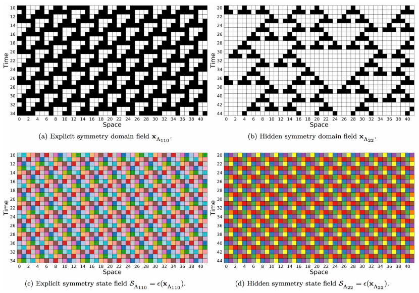
Figure 2: Pure domain spacetime fields for explicit symmetry and hidden symmetry domains shown in (a) and (b) for ECA 110 and ECA 22, respectively. Associated local causal state fields fully display these symmetries in (c) and (d), with each unique color corresponding to a unique local causal state. For ECA 110, lightcone horizons $h^{-}=h^{+}=3$ were used and for rule 22 $h^{-}=10$ and $h^{+}=4$.

IV CA Structures

We now apply the theory of domains and coherent structures to discover patterns in the spacetime fields generated by elementary cellular automata. We first classify ECA domain types. For each class we analyze one exemplar ECA in detail. We begin describing the ECA’s domain(s) and coherent structures generated by the ECA, from both the DPID and local causal state perspectives.

The analysis of domains and structures gives a sense of the correspondence between DPID and the local causal states. The general correspondence, found empirically, between their descriptions of CA domains is as follows. For every known DPID CA domain language, a configuration from the language is used as an initial condition to generate a pure domain field $\mathbf{{x}}_{\Lambda}$. We see that the spacetime shift operators over $\mathcal{S}_{\Lambda}=\epsilon(\mathbf{{x}}_{\Lambda})$ form symmetry groups with the same spatial period, temporal period, and recurrence time as the DPID domain language.

Though the CA dynamic $\Phi$ is not directly used to infer local causal states, the correspondence between DPID and local causal state domains shows that local causal states incorporate detailed dynamical features and they can be used to discover patterns and structures that can be defined directly from $\Phi$ using DPID.

IV.1 CA domains and their classification

ECA domains fall into one of two categories: explicit symmetry or hidden symmetry. In the local causal state formulation, a domain $\Lambda$ has explicit symmetry if the space and time shift operators, $\sigma_{p}$ and $\{\sigma^{s_{n}}\}$, which generate the domain symmetry group over $\mathcal{S}_{\Lambda}=\epsilon(\mathbf{{x}}_{\Lambda})$, also generate that same symmetry group over $\mathbf{{x}}_{\Lambda}$. That is, $\sigma_{p}(\mathbf{{x}}_{\Lambda})=\mathbf{{x}}_{\Lambda}$ and $\sigma^{s_{n}}(\mathbf{{x}}_{\Lambda})=\mathbf{{x}}_{\Lambda}$, for all $n$. From this, we can see that explicit symmetry domains are periodic orbits of the CA, with the domain period equal to the orbit period. This follows since time shifts of the CA spacetime field are essentially equivalent to applying the CA dynamic $\Phi$; $\mathbf{{x}}_{t+p}=\sigma_{p}(\mathbf{{x}})_{t}$ and $\mathbf{{x}}_{t+p}=\Phi^{p}(\mathbf{{x}}_{t})$. Thus, let ${x}_{\Lambda}$ be any spatial configuration of a domain spacetime field, ${x}_{\Lambda}=(\mathbf{{x}}_{\Lambda})_{t}$, for any $t$, then $\Phi^{p}({x}_{\Lambda})={x}_{\Lambda}$ if and only if $\sigma_{p}(\mathbf{{x}}_{\Lambda})=\mathbf{{x}}_{\Lambda}$.

A hidden symmetry domain is one for which the time and space shift operators, that generate the domain symmetry group over $\mathcal{S}_{\Lambda}$, do not generate a symmetry group over $\mathbf{{x}}_{\Lambda}$: $\sigma_{p}(\mathbf{{x}}_{\Lambda})\neq\mathbf{{x}}_{\Lambda}$ or $\sigma^{s_{n}}(\mathbf{{x}}_{\Lambda})\neq\mathbf{{x}}_{\Lambda}$ or both.

In the DPID formulation, a domain is classified as having explicit or hidden symmetry based on the algebra of the domain languages. In this, group elements are the strings of the spatial languages of the domain and the group action is concatenation of the strings. If this algebra for every domain phase $\Lambda_{i}$ is a proper group, $\Lambda$ has explicit symmetry. Otherwise, if the algebra is something more general, like a semigroup or monoid, $\Lambda$ has hidden symmetry. Notably, hidden symmetry domains are associated with a level of stochasticity in the raw spacetime field. We sometimes refer to these as stochastic domains. As the above domain algebra is only used for classification here, we will not give the explicit mathematics. See Refs. [12, App. D] or [70] for those details.

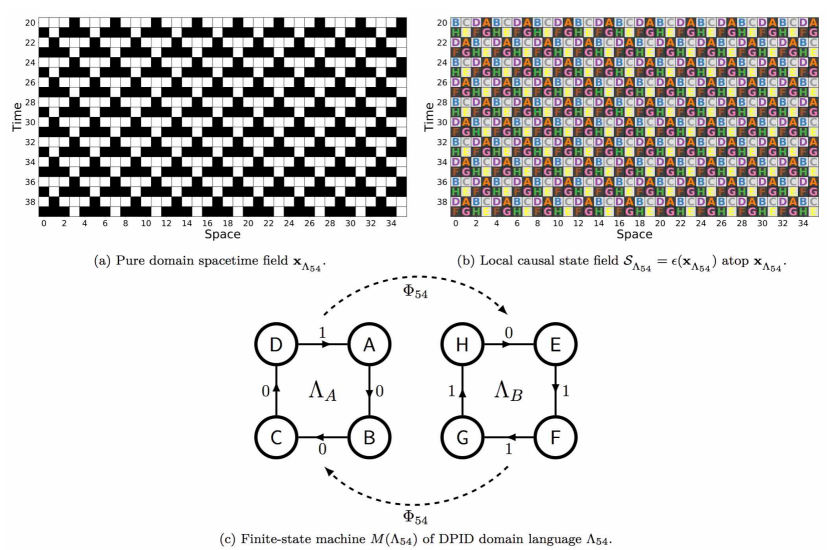
Figure 3: ECA 54 domain: A sample pure domain spacetime field $\mathbf{{x}}_{\Lambda}$ is shown in (a). This field is repeated with the associated local causal states $\mathcal{S}_{\Lambda}=\epsilon(\mathbf{{x}}_{\Lambda})$ added in (b). Lightcone horizons $h^{-}=h^{+}=3$ were used. The DPID spacetime invariant set language is shown in (c). (Reprinted from Ref. [55] with permission.)

Example domains from each category are shown in Figure 2. ECA 110 is given as the explicit symmetry example; a sample spacetime field $\mathbf{{x}}_{\Lambda_{110}}$ of its domain is shown in Figure 2(a). The associated local causal state field $\mathcal{S}_{\Lambda_{110}}$ is shown in Figure 2(c). Each unique color corresponds to a unique local causal state. The local causal state field clearly displays the domain’s translation symmetries. ECA 110’s domain has spatial period $s=14$ and temporal period $p=7$. These are gleaned by direct inspection of the spacetime diagram. Pick any color in $\mathcal{S}_{\Lambda_{110}}$ and one must go through $13$ other colors moving through space to return to the original color and, likewise, $6$ other colors in time before returning. One can also see that at every time step $\mathcal{S}_{\Lambda_{110}}$ has a single spatial tiling $w$ of the $14$ states. Thus, the recurrence time is $\widehat{p}=1$. Finally, notice from Figure 2(a) that spatial configurations of $\mathbf{{x}}_{\Lambda_{110}}$ are periodic orbits of $\Phi_{110}$, with orbit period equal to the domain period, $p=7$.

For a prototype hidden symmetry domain, ECA 22 is used. Crutchfield and McTague used DPID analysis to discover this ECA’s domain in an unpublished work [104] that we used here to produce the domain spacetime field $\mathbf{{x}}_{\Lambda_{22}}$ shown in Figure 2(b). The associated causal state field $\mathcal{S}_{\Lambda_{22}}$ is shown in Figure 2(d). Unlike ECA 110’s domain, it is not clear from $\mathbf{{x}}_{\Lambda_{22}}$ what the domain symmetries are. It is not even clear there are symmetries present from the raw spacetime field. However, the causal state field $\mathcal{S}_{\Lambda_{22}}$ is immediately revealing. Domain translation symmetries are clear. The domain is period $4$ in both space and time: $p=s=4$. There are eight unique local causal states in $\mathcal{S}_{\Lambda_{22}}$ and, as the spatial period is $4$, the eight states come in two distinct spatial tilings $w_{1}$ and $w_{2}$, each consisting of $4$ states. And so, the recurrence time for ECA 22 is $\widehat{p}=2$. Shortly, we examine hidden symmetries in more detail to illustrate how the local causal states lend a new semantics that exposes stochastic symmetries.

Having given concrete demonstrations of the new local causal state formulation of domains and their classification in CAs, we move on to more detailed examples that have been thoroughly studied from the DPID perspective. In doing so, we will see the strong correspondence between the two approaches, in terms of both domains as well as the coherent structures which form atop the domains.

IV.2 Explicit symmetries

We start with a detailed look at ECA 54, whose domains and structures were worked out in detail via DPID [55]. ECA 54 was said to support “artificial particle physics” and this emergent “physics” was specified by the complete catalog of all its particles and their interactions. Here, we analyze the domain and structures using local causal states and compare. Since the particles (structures) are defined as deviations from a domain that has explicit symmetries, the resulting higher-level particle dynamics themselves are completely deterministic. As we will see later, this is not the case for hidden symmetry systems; stochastic domains give rise to stochastic structures.

IV.2.1 ECA 54’s domain

A pure-domain spacetime field $\mathbf{{x}}_{\Lambda}$ of ECA 54 is shown in Fig. 3(a). As can be seen, it has explicit symmetries and is period $4$ in both time and space. From the DPID perspective, though, it consists of two distinct spatial-configuration languages, $\Lambda_{A}=(0001)^{*}$ and $\Lambda_{B}=(1110)^{*}$, that map into each other under $\Phi_{54}$; see Fig. 3(c). This gives a recurrence time of $\widehat{p}=2$. The finite-state machines, $M(\Lambda_{A})$ and $M(\Lambda_{B})$, shown there for these languages each have four states, reflecting the period-$4$ spatial translation symmetry: $s=4$. Although the domain’s recurrence time is $\widehat{p}=2$, the raw states $\mathbf{{x}}_{t}$ are period $4$ in time due to a spatial phase slip in the language evolution: $p=4$. This is shown explicitly in the spacetime machine given in Ref. [55]. We can see that the machine in Fig. 3(c) fully describes the domain field in Fig. 3(a). At some time $t$, the system is either in $(0001)^{*}$ or $(1110)^{*}$ and at the next time step $t+1$ it switches, then back again at $t+2$, and so on.

Let’s compare this with the local causal state analysis. The corresponding local causal state field $\mathcal{S}_{\Lambda}=\epsilon(\mathbf{{x}}_{\Lambda})$ was generated from the pure domain field $\mathbf{{x}}_{\Lambda}$ of Fig. 3(a) via causal filtering; see Fig. 3(b). We reiterate here that this reconstruction in no way relies upon the invariant set languages of $\Lambda_{54}$ identified in DPID. Yet we see that the local causal states correspond exactly to $M(\Lambda_{54})$’s states. In total there are eight states, and these appear as two distinct tilings in the field. These tilings correspond to the two temporal phases of $\Lambda_{54}$: $w_{A}=[\sf{A},\sf{B},\sf{C},\sf{D}]=$ $\Lambda_{A}$ and $w_{B}=[\sf{E},\sf{F},\sf{G},\sf{H}]=$ $\Lambda_{B}$. At any given time $t$, a spatial configuration is tiled by only one of these temporal phases, which each consist of $4$ states, giving a spatial period $s=4$. And, at the next time $t+1$ there are only states from the other tiling. Then back to previous tiling, and so, the evolution continues. Thus, we can see the recurrence time is $\widehat{p}=2$. In contrast, the actual local causal states are temporally period $p=4$, which is also the orbit period of configurations in $\mathbf{{x}}_{\Lambda}$, as can be seen in Fig. 3(a). This is in agreement with DPID’s invariant set analysis, shown in Fig. 3(c). As noted before and as will be emphasized, there is a strong correspondence between DPID’s dynamically invariant sets of spatially homogeneous configurations and the local causal state description, both for coherent structures and the domains from which they are defined.

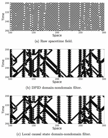
Figure 4: Overview of ECA 54 structures: (a) A sample spacetime field evolved from a random initial configuration. (b) A filter that outputs white for cells participating in domains and black otherwise, using the DPID definition of domain. (c) The analogous domain-nondomain filter that uses the local causal state definition of domain. Lightcone horizons $h^{-}=h^{+}=3$ were used.

IV.2.2 ECA 54’s structures

Let’s examine the structures (particles) supported by ECA 54 and their interactions. Rule 54 organizes itself into domains and structures when started with random initial conditions. A sample spacetime field $\mathbf{{x}}$ produced by evolving a random binary configuration under $\Phi_{54}$ is shown in Fig. 4(a). We first give a qualitative comparison of the structures in this field from both the DPID and local causal state perspectives.

From the DPID side, a simple domain-nondomain filter is used with binary outputs that flag sites in transducer filter field $T=\tau(\mathbf{{x}})$ as either domain (white) or not domain (black). Applying this filter to the spacetime field of Fig. 4(a) generates the diagram shown in Fig. 4(b). Similarly, a domain-nondomain filter built from local causal states when applied to Fig. 4(a) gives the output shown in Fig. 4(c). For this filter, the eight domain local causal states in $\mathcal{S}=\epsilon(\mathbf{{x}})$ are in white and all other local causal states black. While domain-nondomain detections differ site-by-site, we see that in aggregate there is again strong agreement on the structures identified by the two filter types.

There are four types of particles found in ECA 54 [55], which we can now examine in detail. Before doing so, we must make a comment about the domain transducer $\tau$ used by DPID to identify structures. As mentioned, a stack automaton is generally required, but may be well-approximated with a finite-state transducer [56]. A trade-off is made with the transducer, however, since it must choose a direction to scan configurations—left-to-right or right-to-left. To best capture the proper spatial extent of a particle, an interpolation may be done by comparing right and left scans. This was done in the domain-nondomain filter of Fig. 4(b). The bidirectional interpolation used does not capture fine details of domain deviations. For the particle analysis that follows, a single direction (left to right) scan is applied to produce each $T_{t}=\tau(\mathbf{{x}}_{t})$ in $T=\tau(\mathbf{{x}})$. A noticeable side-effect of the single direction scan is that it covers only about half of any given particle’s spatial extent. (This scan-direction issue simply does not arise in local causal state filtering.)

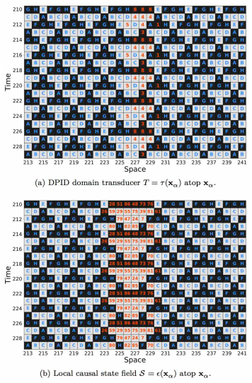
Figure 5: ECA 54’s $\alpha$ particle: In both (a) and (b) white ($0$) and black ($1$) squares display the underlying ECA spacetime field $\mathbf{{x}}_{\alpha}$. (a) The DPID domain transducer filter $T=\tau(\mathbf{{x}}_{\alpha})$ output is overlaid atop the spacetime field values of $\mathbf{{x}}_{\alpha}$. Blue letters are sites participating in domain and red numbers are particular deviations from domain. (b) The local causal state field $\mathcal{S}=\epsilon(\mathbf{{x}}_{\alpha})$. The eight domain states are given by blue letters, all others by red numbers. In both diagrams, the non-domain sites outline the $\alpha$ particle of rule 54, according to the two different semantic filters. Lightcone horizons $h^{-}=h^{+}=3$ were used.

The first structure we analyze is the large stationary $\alpha$ particle, shown in Fig. 5. For both diagrams the white and black squares represent the values $0$ and $1$, respectively, of the underlying ECA field $\mathbf{{x}}_{\alpha}$. Overlaid blue letters and red numbers are the semantic filter fields. In Fig. 5(a) these come from the DPID domain transducer filtered field $T=\tau(\mathbf{{x}}_{\alpha})$. In Fig. 5(b) they come from the local causal state field $\mathcal{S}=\epsilon(\mathbf{{x}}_{\alpha})$.

For the DPID domain transducer filtered field in Fig. 5(a), overlaid blue letters are sites flagged as participating in domain by the transducer $\tau$, with the letter representing the spatial phase of the domain as given by $M(\Lambda_{54})$. Red numbers correspond to sites flagged as various deviations from domain [55]. Here, the collection of such deviations outlines the $\alpha$ particle’s structure; though, as stated above, the unidirectional transducer only identifies about half of the particle’s spatial extent. The main feature to notice is that the particle has a period-$4$ temporal oscillation. As the $\alpha$ is recognizable by eye from the raw field values, one can see this period-$4$ structure is intrinsic to the raw spacetime field and not an artifact of the domain transducer. However, the period-$4$ temporal structure is clearly displayed by the DPID domain transducer description of $\alpha$.

Figure 5(b) displays the local causal state field $\mathcal{S}=\epsilon(\mathbf{{x}}_{\alpha})$; the eight domain states are given as blue letters, following Fig. 3(b), and all other nondomain states, which outline the $\alpha$, are red numbers. We see the local causal states fill out the $\alpha$’s full spatial extent. Since the numeric labels for each state are arbitrarily assigned during reconstruction, the $\alpha$’s spatial reflection symmetry that is clearly present does not appear in the local causal state labels. However, the underlying lightcones that populate the equivalence classes of these states do exhibit this symmetry. As with the DPID domain transducer description though, the local causal states properly capture the $\alpha$’s temporal period-$4$.

We emphasize that coherent structures are behaviors of the underlying system and, as such, they exist in the system’s spacetime field. The semantic filter fields are formal methods that identify sites in the underlying spacetime field which participate in a particular structure. This is how overlay diagrams, like Fig. 5, derive their utility.

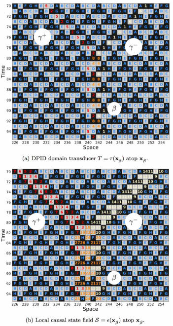
Figure 6: ECA 54’s $\gamma^{+}+\gamma^{-}\rightarrow\beta$ interaction: In both diagrams the white ($0$) and black ($1$) squares display the underlying ECA spacetime field $\mathbf{{x}}_{\beta}$. (a) The DPID domain transducer filter $T=\tau(\mathbf{{x}}_{\beta})$ output is overlaid atop the spacetime field values of $\mathbf{{x}}_{\beta}$. Blue letters are sites identified by $T$ as participating in the domain. Colored numbers are sites identified as participating in one of the three remaining structures. The $\gamma^{+}$ particle is outlined only by red numbers, $\gamma^{-}$ by yellow numbers, and $\beta$ by a combination of red, yellow, and orange. (b) The local causal state field $\mathcal{S}=\epsilon(\mathbf{{x}}_{\beta})$ is overlaid atop $\mathbf{{x}}_{\beta}$. The eight domain states are in blue, and the other nondomain states are colored the same as in (a). Lightcone horizons $h^{-}=h^{+}=3$ were used.

We discuss the three remaining structures of ECA 54 by examining an interaction among them; the left-traveling $\gamma^{-}$ particle can collide with the right-traveling $\gamma^{+}$ particle to form the $\beta$ particle. This interaction is displayed with overlay diagrams in Fig. 6. The values of the underlying field $\mathbf{{x}}_{\beta}$ are given by white ($0$) and black ($1$) squares. The DPID domain transducer filter field $T=\tau(\mathbf{{x}}_{\beta})$ is overlaid over top of $\mathbf{{x}}_{\beta}$ in Fig. 6(a) and the local causal state field $\mathcal{S}=\epsilon(\mathbf{{x}}_{\beta})$ atop $\mathbf{{x}}_{\beta}$ in Fig. 6(b).

In both cases, the color scheme is as follows. Sites identified by the semantic filters as participating in a domain are colored blue, with the letters specifying the particular phase of the domain. In Fig. 6(a) the domain phases are specified by $T$ and in Fig. 6(b) they are specified by $S$. And, as we saw in Fig. 3 and can see here, these specifications of $\Lambda_{54}$ are identical. For both Figs. 6(a) and 6(b), nondomain sites participating in the $\gamma^{+}$ are flagged with red, those participating in the $\gamma^{-}$ with yellow, and those uniquely participating in the $\beta$ with orange.

As with the $\alpha$ particle, the local causal state description better covers the particles’ spatial extent, but both filters agree on the temporal oscillations of each particle. Both $\gamma$s are period $2$ and $\beta$ is period $4$. Unlike the $\alpha$ and $\beta$, the $\gamma$ particles are not readily identifiable by eye. They arise as a result of a phase slip in the domain. For example, a spatial configuration with a $\gamma$ present is of the form $\Lambda_{A}\;\gamma\;\Lambda_{B}$.

Related to this, we point out here an observation about this interaction that illustrates how our methods uncover structures in spatiotemporal systems. At the top of each diagram in Fig. 6 the spatial configurations are of the form $\Lambda_{A}\;\gamma^{+}\;\Lambda_{B}\;\gamma^{-}\;\Lambda_{A}$. At each subsequent time step, the domains change phase $A\rightarrow B$ and $B\rightarrow A$ and the intervening domain region shrinks as the $\gamma$s move towards each other. The intervening domain disappears when the $\gamma$s finally collide. Then we have local configurations of the form $\Lambda_{A}\;\beta\;\Lambda_{A}$. However, there is an indication that a phase slip between these domain regions still happens “inside” the $\beta$ particle. Notice in Fig. 6 there are several spatial configurations (horizontal time slices) in which domain states appear inside the $\beta$ that are the opposite phase of the bordering domain phases, indicating a phase slip. Also, the states constituting the $\gamma$s are found as constituents of the $\beta$. For the DPID domain transducer $\tau$, each $\gamma$ consists of just two states, and all four of these states (two for each $\gamma$) are found in the $\beta$. In the local causal state field $S$, each $\gamma$ is described by eight local causal states. Not all of these show up as states of the $\beta$, but several do. Those $\gamma$ states that do show up in the $\beta$ appear in the same spatiotemporal configurations they have in the $\gamma$s.

These observations tell us about the underlying ECA’s behavior and so can be gleaned from the raw spacetime field itself. That said, the discovery that the $\beta$ particle is a “bound state” of two $\gamma$s and that it contains an internal phase slip of the bordering domain regions is not at all obvious from inspecting raw spacetime fields. That is, $\gamma^{+}\;\Lambda\;\gamma^{-}\rightarrow\beta$. Such structural discovery, however, is greatly facilitated by the coherent structure analysis. To emphasize, these insights concern the intrinsic organization embedded in the spacetime fields generated by the ECA. No structural assumptions, beyond the very basic definitions of local causal states, are required.

Let’s recapitulate the correspondence between the independent DPID and local causal state descriptions of the ECA 54 domain and structures. From the DPID perspective, the ECA 54 domain $\Lambda_{54}$ consists of two homogeneous spatial phases that are mapped into each other by $\Phi_{54}$. In contrast, $\Lambda_{54}$ is described by a set of local causal states with a spacetime translation symmetry tiling. The two descriptions agree completely, giving a spatial period $4$, temporal period $4$, and recurrence time of $2$. On the one hand, for ECA $54$’s structures DPID directly uses domain information to construct a transducer filter $T=\tau(\mathbf{{x}})$ that identifies structures as groupings of particular domain deviations. On the other, the local causal states are assigned uniformly to spacetime field sites via causal filtering $\mathcal{S}=\epsilon(\mathbf{{x}})$. Domains and sites participating in a domain are found by identifying spatiotemporal symmetries in the local causal states. Coherent structures are then localized deviations from these symmetries. Though the agreement is not exact as with the domain, DPID and the local causal states still agree to a large extent on their descriptions of ECA 54’s four particles and their interactions.

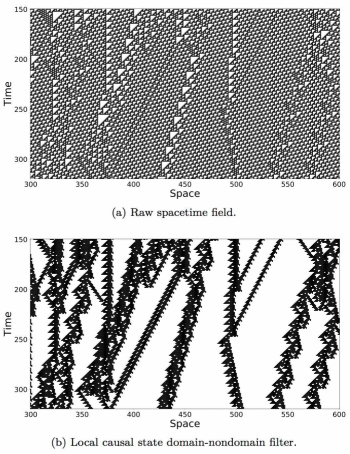
Figure 7: ECA 110 structures: (a) A sample field evolved from a random initial configuration. (b) A local causal state domain-nondomain filter with domain sites in white and nondomain in black. Lightcone horizons $h^{-}=h^{+}=3$ were used.

IV.2.3 ECA 110

As the most complex explicit symmetry ECA, ECA 110 is worth a brief mention. It is the only ECA proven to support universal computation (on a specific subset of initial configurations) and implements this using a subset of the ECA’s coherent structures [89]. This was shown by mapping ECA 110’s particles and their interactions onto a cyclic tag system that emulates a Post tag system which, in turn, emulates a universal Turing machine. A domain-nondomain filter reveals several of ECA 110’s particles used in the implementation; see Fig. 7. The ECA 110 domain was displayed in Figs. 2(a) and 2(c), as the example for explicit symmetry domains. The domain has a single phase, rather than two phases like ECA 54’s, and requires $14$ states, as opposed to ECA 54’s combined $8$. The ECA 110’s highly complex behavior surely derives from the heightened complexity of its domain. Exactly how, though, remains an open problem.

IV.3 Hidden stochastic symmetries

Our attention now turns to ECAs with hidden symmetries and stochastic domains. These are the so-called “chaotic” ECAs. Since the structure of an ECA’s domain heavily dictates the overall behavior, stochastic domains give rise to stochastic structures and hence, in combination, to an overall stochastic behavior. To be clear, since all ECA dynamics are globally deterministic—the evolution of spatial configurations is deterministic—the stochasticity here refers to local structures rather than global configurations. In contrast to explicit symmetry ECAs whose structures are largely identifiable from the raw spacetime field, the structures found in stochastic-domain ECAs are often not at all apparent. In this case the ability of our methods to facilitate the discovery and description of such hidden structures is all the more important and sometimes even necessary. While the distinction between stochastic and explicit symmetry domains does not make a difference when determining DPID’s spacetime invariant sets, local causal state inference is relatively more difficult with stochastic domains, usually requiring large lightcone depths and an involved domain-structure analysis.

Here, we examine ECA 18 in detail, as its stochastic domain is relatively simple and well understood. An empirical domain-structure analysis of ECA 18 was first given in Ref. [105] and then more formally in Refs. [106, 107, 108, 109], which notes the domain’s temporal invariance. It was not until the FME was introduced in Ref. [50] that this was rigorously proven and shown to follow within the more DPID general framework. The distinguishing feature of ECA 18’s domain observed in the early empirical analysis was that the lookup table $\phi_{18}$ becomes additive when restricted to domain configurations. Specifically, when restricted to domain, $\phi_{18}$ is equivalent to $\phi_{90}$, which is the sum mod $2$ of the outer two bits of the local neighborhood; $\mathbf{{x}}_{t+1}^{r}=\phi_{90}(\mathbf{{x}}_{t}^{r-1}\mathbf{{x}}_{t}^{r}\mathbf{{x}}_{t}^{r+1})=\mathbf{{x}}_{t}^{r-1}+\mathbf{{x}}_{t}^{r+1}\;(\mathrm{mod}\;2)$.

ECA 18’s structures illustrate additional complications of local causal state analysis with stochastic symmetry systems. Nondomain states of ECA 54 and other explicit symmetry ECAs always indicate a particle or particle interaction, after transients. This is not the case with chaotic ECAs, and our formal definition is needed to identify ECA 18’s coherent structures.

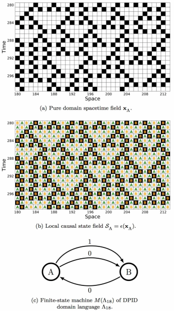
Figure 8: ECA 18 domain: (a) Iterates of a sample pure domain spacetime field $\mathbf{{x}}_{\Lambda}$, white and black are values $0$ and $1$, respectively. (b) The same domain field with the local causal state field $\mathcal{S}_{\Lambda}=\epsilon(\mathbf{{x}}_{\Lambda})$ overlaid. Lightcone horizons $h^{-}=8$ and $h^{+}=3$ were used. (c) The finite-state machine $M(\Lambda_{18})$ of the DPID invariant set language of the ECA 18 domain $\Lambda_{18}$. (Reprinted with permission from Ref [50].)

IV.3.1 ECA 18’s domain

Iterates of a pure domain spacetime field $\mathbf{{x}}_{\Lambda_{18}}$ for the ECA 18 domain $\Lambda_{18}$ is shown in Fig. 8(a). White and black cells represent site values $0$ and $1$, respectively. A symmetry is not apparent in the spacetime field. One noticeable pattern, though, is that $1$s (black cells) always appear in isolation, surrounded by $0$s on all four sides. This still does not reveal symmetry, since neither time nor space shifts match the original field. When scanning along one dimension, making either timelike or spacelike moves (vertically or horizontally), one sees that every other site is always a $0$ and the sites in between are wildcards—they can be either $0$ or $1$. Making this identification finally reveals the symmetry in the ECA 18 domain [50].

In contrast to this ad hoc description, the $0$-wildcard pattern is clearly and immediately identified in the local causal state field $\mathcal{S}_{\Lambda}=\epsilon(\mathbf{{x}}_{\Lambda})$, shown in Figure 8(b). State $A$ occurs on the fixed-$0$ sites and state $B$ on the wildcard sites. And, these states occur in a checkerboard symmetry that tiles the spacetime field. An interesting observation of this symmetry group is that it has rotational symmetry, in addition to the time and space translation symmetries. This is a rotation, though, in spacetime. While unintuitive at first, the above discussion shows this spacetime rotational symmetry is not just a coincidence. The $0$-wildcard semantics applies for both spacelike and timelike scans through the field.

The DPID invariant-set language for this domain is given in Figure 8(c). Not surprisingly, this is the $0$-wildcard language. It is easy to see that $\phi_{18}$ creates a tiling of $0$-wildcard local configurations. Also, note the transition branching (the wildcard) leaving state $A$ indicates a semigroup algebra. This identifies $\Lambda_{18}$ as a stochastic symmetry domain. We again see a clear correspondence between the local causal state identification of the domain and that of DPID. Both give spatial period $s=2$, temporal period $p=2$, and recurrence time $\widehat{p}=1$, as there is a single local causal state tiling and a single DPID spatial language, both corresponding to the $0$-wildcard pattern.

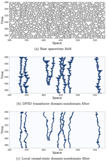
Figure 9: ECA 18 structures: (a) Sample spacetime field evolved under ECA 18 from a random initial configuration. (b) Spacetime field after filtering with domain regions in white and coherent structures in blue, using the DPID domain transducer. (c) Spacetime field filtered with domain regions in white and structures in blue, using local causal states. The occasional gap in the structures is an artifact of using finite-depth lightcones during reconstruction of local causal states. Lightcone horizons $h^{-}=8$ and $h^{+}=3$ were used.

IV.3.2 ECA 18’s structures

ECA 18’s two-state domain $\Lambda_{18}$ supports a single type of coherent structure—the $\alpha$ particle that appears as a phase-slip in the spatial period-$2$ domain and consists of local configurations $10^{2k}1$, $k=0,1,2,\ldots$. The domain’s stochastic nature drives the $\alpha$s in an unbiased left-right random-walk. When two collide they pairwise annihilate; resolving each $\alpha$’s spatial phase shift. To clarify, the $\alpha$ of ECA 18 has no relation to the $\alpha$ of ECA 54.

Figure 9 shows these structures as they evolve from a random initial configuration under $\Phi_{18}$. The raw spacetime field is given in Fig. 9(a) with the DPID transducer domain-nondomain filter (bidirectional scan interpolation) in Fig. 9(b) and the local causal state domain-nondomain filter in Fig. 9(c). With the aid of these domain filters, visual inspection shows that ECA 18’s structures are, in fact, pairwise annihilating random-walking particles. This was explored in detail by Ref. [52].

As noted above, the domain-structure local causal state analysis for stochastic domain systems is generally more subtle. In the DPID analysis, ECA 18 consists solely of the single domain and random-walking $\alpha$ particle structures. Thus, using the DPID transducer to filter out sites participating in domains leaves only $\alpha$ particles, as done in Fig. 9(b). The situation is more complicated in the local causal state analysis. As described in more detail shortly, filtering out domain states leaves behind more than the structures. Why exactly this happens is the subject of future work. The field shown in Fig. 9(c) was produced from a coherent structure filter, rather than from a domain-nondomain filter. There, local causal states that fit the coherent structure criteria are colored blue and all others are colored white.

To illustrate the more involved local causal state analysis let’s take a closer look at the $\alpha$ particle. This also highlights a major difference between DPID and local causal state analyses. As the DPID transducer is strictly a spatial description it can identify structures that grow in a single time step to arbitrary size. One artifact of this is that the spatial growth can exceed the speed of local information propagation and thus make structures appear acausal. The local causal states, however, are constructed from lightcones and so naturally take into account this notion of causality. They cannot describe such acausal structures. Accounting for this, though, there is a strong agreement between the two descriptions.

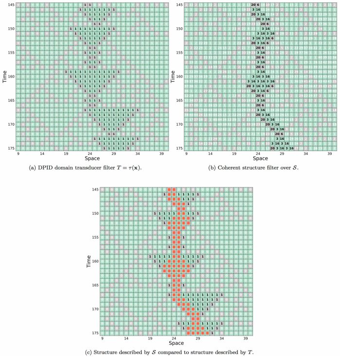
Figure 10: Comparative analysis of ECA 18’s $\alpha$ particle: In all three spacetime diagrams, the underlying ECA field values of $0$ and $1$ are represented as green and gray squares, respectively. (a) DPID domain transducer filtered field $T=\tau(\mathbf{{x}})$ with bidirectional scan interpolation. Domain sites are identified with white $0$s and particle sites with black $1$s. (b) A coherent structure causal filter; local causal state field $\mathcal{S}=\epsilon(\mathbf{{x}})$ with nondomain local causal states states satisfying the coherent structure definition are colored black with all other states colored white. Lightcone horizons $h^{-}=8$ and $h^{+}=3$ were used. (c) Comparison of the structures from the two methods: The DPID transducer filter of (a) with sites that have local causal states identified as the coherent structure in (b) given a red square label.

From the perspective of the DPID domain transducer $\tau$ ECA 18’s $\alpha$ particles are simple to understand. From the domain language in Fig. 8(c), the domain-forbidden words are those in the regular expression $1(00)^{*}1$. That is, pairs of ones with an even number of $0$s (including no $0$s) in between. This is the description of $\alpha$ particles at the spatial configuration level. The DPID bidirectional scan interpolation domain transducer perfectly captures $\alpha$ described this way; see Fig. 10(a). To aid in visual identification we employed a different color scheme for Fig. 10: the underlying ECA field values are given by green ($0$) and gray ($1$) squares. For the DPID transducer filtered field $T=\tau(\mathbf{{x}})$ in Fig. 10(a), overlaid white $0$s identify domain sites and black $1$s identify particle sites. Every local configuration identified as an $\alpha$ is of the form $1(00)^{*}1$. As noted above, however, $\alpha$s described in this way can grow in size arbitrarily in a single time step as the number of pairs of zeros in $1(00)^{*}1$ is unbounded.

Local causal state inference—whether topological [86] or probabilistic [49]—is unsupervised in the sense that it uses only raw spacetime field data and no other external information such as the CA rule used to create that spacetime data. Once states are inferred, further steps are needed for coherent structure analysis.

The first step is to identify domain states in the local causal state field $\mathcal{S}=\epsilon(\mathbf{{x}})$. They tile spacetime regions, i.e., domain regions. For explicit-symmetry domain ECAs this step is sufficient for creating a domain-structure filter. Tiled domain states can be easily identified and all other states outline ECA structures or their interactions. The situation is more subtle, however, for ECAs with stochastic domains. A detailed description of the implementation of additional “decontamination” steps is given in a sequel.

For our purposes here, though, it suffices to strictly apply the definition of coherent structures after this first “out of the box” unsupervised causal filter. The initial unsupervised filtered spacetime diagram identifies a core set of states that are spatially localized and temporally persistent. A coherent structure filter then isolates these states by coloring them black and all other states white in the local causal state field $\mathcal{S}$. The output of this filter is shown in Fig. 10(b). The growth rate of the structures identified in this way—by the local causal states—is limited by the speed of information propagation, which for ECAs is unity. Applying this growth-rate constraint on the DPID structure transducer, one again finds strong agreement. A comparison is shown in Fig. 10(c). It shows the output of the DPID filter applied to the spacetime field of Fig. 10(a) and, in red, sites corresponding to the structure according to the local causal states in Fig. 10(b).

V Discussion

Having laid out our coherent structure theory and illustrating it in some detail, it is worth looking back, as there are subtleties worth highlighting. The first is our use of the notion of semantics, which derives from the measurement semantics introduced in Ref. [87]. Performing causal filtering $\mathcal{S}=\epsilon(\mathbf{{x}})$ may at first seem counterproductive, especially for binary fields like those generated by ECAs, as the state space of the system is generally larger in $\mathcal{S}$ than in $\mathbf{{x}}$. As the local state space of ECAs is binary, complexity is manifest in how the sites interact and arrange themselves. Not all sites in the field play the same role. For instance, in ECA 110’s domain, Fig. 2(a), the $0$s in the field group together to form a triangular shape. This triangle has a bottom-most $0$ and a rightmost $0$, but they are both still $0$s. To capture the semantics of “bottom-most” and “rightmost” $0$ of that triangle shape, a larger local state space is needed. And, indeed, this is exactly the manner in which the local causal states capture the semantics of the underlying field. We saw a similar example with the fixed-$0$ and wildcard semantics of $\Lambda_{18}$.

The values in the fields $\mathcal{S}=\epsilon(\mathbf{{x}})$ and $T=\tau(\mathbf{{x}})$ are not measures of some quantity, but rather semantic labels. For the local causal states, they are labels of equivalence classes of local dynamical behaviors. For the DPID domain transducer, they label sites as being consistent with the domain language $\Lambda$ or else as the particular manner in which they deviate from that language.

This, however, is only the first level of semantics used in our coherent structure theory. While the filtered fields $\mathcal{S}=\epsilon(\mathbf{{x}})$ and $T=\tau(\mathbf{{x}})$ capture semantics of the original field $\mathbf{{x}}$, to identify coherent structures a new level of semantics on top of these filtered fields is needed. These are semantics that identify sites as domain or coherent structure using $\mathcal{S}$ and $T$. For the DPID domain transducer $T$, the domain semantics are by construction built into $T$. Our coherent structure definition adds the necessary semantics to identify collections of nondomain sites as participating in a coherent structure.

For the local causal states, one may think of the field $\mathcal{S}=\epsilon(\mathbf{{x}})$ as being the semigroup level of semantics. That is, they represent pattern and structure as generalized symmetries of the underlying field $\mathbf{{x}}$. This is the same manner in which the $\epsilon$-machine captures pattern and structure of a stochastic process with semigroup algebra [87]. The next level of semantics, used to identify domains, requires finding explicit symmetries in $\mathcal{S}$. Thus, domain semantics are the group-theoretic level of semantics, since domains are identified by spacetime translation symmetry groups over $\mathcal{S}$. With states participating in those symmetry groups identified, our coherent structure definition again provides the necessary semantics to identify structures in $\mathbf{{x}}$ through $\mathcal{S}$. These remarks hopefully also clarify the interplay between group and semigroup algebras in our development.

Lastly, we highlight the distinction between a CA’s local update rule $\phi$ and its global update $\Phi$—the CA’s equations of motion. For many CAs, as with ECAs, $\Phi$ is constructed from simultaneous synchronous application of $\phi$ across the lattice. In a sense, then, there is a simple relation between $\phi$ and $\Phi$. However, as demonstrated by many ECAs, most notably the Turing complete ECA 110, the behaviors generated by $\Phi$ can be extraordinarily complicated, even though $\phi$ is extraordinarily simple. This is why complex behaviors and structures generated by ECAs are said to be emergent.

This point is worth emphasizing here due to the relationship between past lightcones and $\phi^{i}$ for CAs. Since the local causal states are equivalence classes of past lightcones, they are equivalence classes of the elements of $\phi^{i}$ for CAs. Thus, the system’s local dynamic is directly embedded in the local causal states. As we saw, the local causal states are capable of capturing emergent behaviors and structures of CAs and so, in a concrete way, they provide a bridge between the simple local dynamic $\phi$ and the emergent complexity generated by $\Phi$. Moreover, the correspondence between the local causal state and DPID domain-structure analysis shows the particular equivalence relation over the elements of $\phi^{i}$ used by the local causal states captures key dynamical features of $\Phi$, used explicitly by DPID.

The relationship, though, between $\phi^{i}$ and $\Phi$ captured by the local causal states is not entirely transparent, as most clearly evidenced by the need for behavior-driven reconstruction of the local causal states. Given a CA lookup table $\phi$, one may pick a finite depth $i$ for the past lightcones and easily construct $\phi^{i}$. It is not at all clear, however, how to use $\Phi$ to generate the equivalence classes over the past lightcones of $\phi^{i}$ that have the same conditional distributions over future lightcones. The only known way to do this is by brute-force simulation and reconstruction, letting $\Phi$ generate past lightcone-future lightcone pairs directly.

VI Conclusions

Two distinct, but closely related, approaches to spatiotemporal computational mechanics were reviewed: DPID and local causal states. From them, we developed a theory of coherent structures in fully discrete dynamical field theories. Both approaches identify special symmetry regions of a system’s spatiotemporal behavior—a system’s domains. We then defined coherent structures as localized deviations from domains; i.e., coherent structures are locally broken domain symmetries.

The DPID approach defines domains as sets of homogeneous spatial configurations that are temporally invariant under the system dynamic. In 1+1 dimension systems, dynamically important configuration sets can be specified as particular types of regular language. Once these domain patterns are identified, a domain transducer $\tau$ can be constructed that filters spatial configurations $T_{t}=\tau(\mathbf{{x}}_{t})$, identifying sites that participate in domain regions or that are the unique deviations from domains. Finding a system’s domains and then constructing domain transducers requires much computational overhead, but full automation has been demonstrated. Once acquired, the domain transducers provide a powerful tool for analyzing emergent structures in discrete, deterministic 1+1 dimension systems. The theory of domains as dynamically invariant homogeneous spatial configurations is easily generalizable beyond this setting, but practical calculation of configuration invariant sets in more generalized settings presents enormous challenges.

The local causal state approach, in contrast, generalizes well. Both in theory and in practice, under a caveat of computational resource scaling. It is a more direct generalization of computational mechanics from its original temporal setting. The causal equivalence relation over pasts based on predictions of the future is the core feature of computational mechanics from which the generalization follows. Local causal states are built from a local causal equivalence relation over past lightcones based on predictions of future lightcones. Local causal states provide the same powerful tools of domain transducers, and more. Being equivalence classes of past lightcones, which in the deterministic setting are the system’s underlying local dynamic, local causal states offer a bridge between emergent structures and the underlying dynamic that generates them.

In both, patterns and structures are discovered rather than simply recognized. No external bias or template is imposed, and structures at all scales may be uniformly captured and represented. These representations greatly facilitate insight into the behavior of a system, insights that are intrinsic to a system and are not artifacts of an analyst’s preferred descriptional framework. ECA 54’s $\gamma^{+}+\Lambda+\gamma^{-}\rightarrow\beta$ interaction exemplifies this.

DPID domain transducers utilize full knowledge of a system’s underlying dynamic and, thus, perfectly capture domains and structures. Local causal states are built purely from spacetime fields and not the equations of motion used to produce those fields. Yet, the domains and structures they capture are remarkably close to the dynamical systems benchmark set by DPID. This is highly encouraging as the local causal states can be uniformly applied to a much wider array of systems than the DPID domain transducers, while at the same time providing a more powerful analysis of coherent structures.

Looking beyond cellular automata, recent years witnessed renewed interest in coherent structures in fluid systems [40, 110, 43]. There has been particular emphasis on Lagrangian methods, which focus on material deformations generated by the flow. The local causal states, in contrast, are an Eulerian approach, as they are built from lightcones taken from spacetime fields and do not require material transport in the system. A frequent objection raised against Eulerian approaches to coherent structures is that such approaches are not “objective”—they are not independent of an observer’s frame of reference. This applies for instantaneous Eulerian approaches, however. And so, does not apply to local causal states. In fact, lightcones and the local causal equivalence relation over them are preserved under Euclidean isometries. This can be seen from Eqs. (1) and (2) that define lightcones in terms of distances only and so they are independent of coordinate reference frame. Local causal states are objective in this sense.

Methods in the Lagrangian coherent structure literature fall into two main categories: diagnostic scalar fields and analytic approaches utilizing one or another mathematical coherence principle. Previous approaches to coherent structures using local causal states relied on the local statistical complexity [57, 58]. This is a diagnostic scalar field and comes with all the associated drawbacks of such approaches [44]. The coherent structure theory presented here, in contrast, is the first principled mathematical approach to coherent structures using local causal states.

With science producing large-scale, high-dimensional data sets at an ever increasing rate, data-driven analysis techniques like the local causal states become essential. Standard machine learning techniques, most notably deep learning methods, convolutional neural nets, and the like are experiencing increasing use in the sciences [111, 112]. Unlike commercial applications in which deep learning has led to surprising successes, scientific data is highly complex and typically unlabeled. Moreover, interpretability and detecting new mechanisms are key to scientific discovery. With these challenges in mind, we offer local causal states as a unique and valuable tool for discovering and understanding emergent structure and pattern in spatiotemporal systems.

References

- [1] M. Minsky. Computation: Finite and Infinite Machines. Prentice-Hall, Englewood Cliffs, New Jersey, 1967.
- [2] N. Chomsky. Three models for the description of language. IRE Trans. Info. Th., 2:113–124, 1956.
- [3] W. Heisenberg. Nonlinear problems in physics. Physics Today, 20:23–33, 1967.
- [4] E. N. Lorenz. Deterministic nonperiodic flow. J. Atmos. Sci., 20:130, 1963.
- [5] E. N. Lorenz. The problem of deducing the climate from the governing equations. Tellus, XVI:1, 1964.
- [6] D. Ruelle and F. Takens. On the nature of turbulence. Comm. Math. Phys., 20:167–192, 1971.
- [7] N. H. Packard, J. P. Crutchfield, J. D. Farmer, and R. S. Shaw. Geometry from a time series. Phys. Rev. Let., 45:712, 1980.
- [8] F. Takens. Detecting strange attractors in fluid turbulence. In D. A. Rand and L. S. Young, editors, Symposium on Dynamical Systems and Turbulence, volume 898, page 366, Berlin, 1981. Springer-Verlag.
- [9] A. Brandstater, J. Swift, Harry L. Swinney, A. Wolf, J. D. Farmer, E. Jen, and J. P. Crutchfield. Low-dimensional chaos in a hydrodynamic system. Phys. Rev. Lett., 51:1442, 1983.
- [10] J. P. Crutchfield and B. S. McNamara. Equations of motion from a data series. Complex Systems, 1:417 – 452, 1987.
- [11] J. P. Crutchfield and K. Young. Inferring statistical complexity. Phys. Rev. Let., 63:105–108, 1989.
- [12] C. R. Shalizi and J. P. Crutchfield. Computational mechanics: Pattern and prediction, structure and simplicity. J. Stat. Phys., 104:817–879, 2001.
- [13] J. P. Crutchfield. Between order and chaos. Nature Physics, 8(January):17–24, 2012.
- [14] J. P. Crutchfield. The calculi of emergence: Computation, dynamics, and induction. Physica D, 75:11–54, 1994.
- [15] P. W. Anderson. More is different. Science, 177(4047):393–396, 1972.
- [16] J. P. Crutchfield. The dreams of theory. WIRES Comp. Stat., 6(March/April):75–79, 2014.
- [17] M. Van Dyke. An Album of Fluid Motion. Parabolic Press, Stanford, California, 1982.
- [18] P. Ball. The Self-Made Tapestry: Pattern Formation in Nature. Oxford University Press, New York, 1999.
- [19] W. G. Flake. The Computational Beauty of Nature: Computer Explorations of Fractals, Chaos, Complex Systems, and Adaptation. Bradford Books, New York, 2000.
- [20] U. Nakaya. Snow Crystals: Natural and Artificial. Harvard University Press, Boston, Massachusetts, 1954.
- [21] E. Ben-Jacob, I. Cohen, O. Shochet, I. Aranson, H. Levine, and L. Tsimring. Complex bacterial patterns. Nature, 373:556–567, 1995.
- [22] I. V. Markov. Crystal Growth for Beginners: Fundamentals of Nucleation, Crystal Growth and Epitaxy. World Scientific, Singapore, third edition, 2017.
- [23] R. Hoyle. Pattern Formation: An Introduction to Methods. Cambridge University Press, New York, 2006.
- [24] M.C. Cross and H.S. Greenside. Pattern Formation and Dynamics in Nonequilibrium Systems. Cambridge University Press, Cambridge, United Kingdom, 2009.
- [25] H. Bénard. Les Tourbillons Cellulaires dans une nappe Liquide Propageant de la Chaleur par Convection: en Régime Permanent. Gauthier-Villars, 1901.
- [26] Lord Rayleigh. On convection currents in a horizontal layer of fluid, when the higher temperature is on the under side. Phil. Mag. (Series 6), 32(192):529–546, 1916.
- [27] V. Steinberg, G. Ahlers, and D. S. Cannell. Pattern formation and wave-number selection by Rayleigh-Bénard convection in a cylindrical container. Physica Scripta, T9:97, 1985.
- [28] G.I. Taylor. Stability of a viscous liquid contained between two rotating cylinders. Phil. Trans. Roy. Soc. Lond. A, 223:289–343, 1923.
- [29] P.R. Fenstermacher, H.L. Swinney, and J.P. Gollub. Dynamical instabilities and the transition to chaotic Taylor vortex flow. J. Fluid Mech., 94(1):103–128, 1979.
- [30] A.M. Zhabotinsky. A history of chemical oscillations and waves. Chaos, 1(4):379–386, 1991.
- [31] A.T. Winfree and S.H. Strogatz. Singular filaments organize chemical waves in three dimensions: I. Geometrically simple waves. Physica D, 8(1):35–49, 1983.
- [32] M. Faraday. On a peculiar class of acoustical figures; and on certain forms assumed by groups of particles upon vibrating elastic surfaces. Phil. Trans. Roy. Soc. Lond., 121:299–340, 1831.
- [33] A. Kudrolli, B. Pier, and J.P. Gollub. Superlattice patterns in surface waves. Physica D, 123(1-4):99–111, 1998.
- [34] L.E. Reichl. A Modern Course in Statistical Physics. Wiley-VCH, Weinheim, Germany, 2016.
- [35] P. Attard. Optimising principle for non-equilibrium phase transitions and pattern formation with results for heat convection. arXiv:1208.5105.
- [36] H. Haken. Information and Self-Organization. Springer, New York, 2016.
- [37] M. C. Cross and P. C. Hohenberg. Pattern formation outside of equilibrium. Rev. Mod. Phys., 65(3):851–1112, 1993.
- [38] M. Golubitsky and I. Stewart. The Symmetry Perspective: From Equilibrium to Chaos in Phase Space and Physical Space, volume 200. Birkhäuser, New York, 2003.
- [39] M. R. Allshouse and T. Peacock. Lagrangian based methods for coherent structure detection. Chaos, 25(9):097617, 2015.
- [40] G. Haller. Lagrangian coherent structures. Ann. Rev. Fluid Mech., 47:137–162, 2015.
- [41] K. A. Emanuel. The theory of hurricanes. Ann. Rev. Fluid Mech., 23(1):179–196, 1991.
- [42] T. Sapsis and G. Haller. Inertial particle dynamics in a hurricane. J. Atmos. Sci., 66(8):2481–2492, 2009.
- [43] P. Holmes, J.L. Lumley, G. Berkooz, and C.W. Rowley. Turbulence, Coherent Structures, Dynamical Systems and Symmetry. Cambridge University Press, Cambridge, United Kingdom, 2012.
- [44] A. Hadjighasem, M. Farazmand, D. Blazevski, G. Froyland, and G. Haller. A critical comparison of Lagrangian methods for coherent structure detection. Chaos, 27(5):053104, 2017.
- [45] F. Vitart, J.L. Anderson, and W.F. Stern. Simulation of interannual variability of tropical storm frequency in an ensemble of GCM integrations. J. Climate, 10(4):745–760, 1997.
- [46] K. Walsh and I.G. Watterson. Tropical cyclone-like vortices in a limited area model: Comparison with observed climatology. J. Climate, 10(9):2240–2259, 1997.
- [47] Prabhat, S. Byna, V. Vishwanath, E. Dart, M. Wehner, W. D. Collins, et al. TECA: Petascale pattern recognition for climate science. In International Conference on Computer Analysis of Images and Patterns, pages 426–436. Springer, 2015.
- [48] C.M. Bishop. Pattern Recognition and Machine Learning. Springer, New York, 2006.
- [49] C.R. Shalizi. Optimal nonlinear prediction of random fields on networks. Discrete Mathematics & Theoretical Computer Science, 2003.
- [50] J. E. Hanson and J. P. Crutchfield. The attractor-basin portrait of a cellular automaton. J. Stat. Phys., 66:1415 – 1462, 1992.
- [51] J. P. Crutchfield. Discovering coherent structures in nonlinear spatial systems. In A. Brandt, S. Ramberg, and M. Shlesinger, editors, Nonlinear Ocean Waves, pages 190–216, Singapore, 1992. World Scientific. also appears in Complexity in Physics and Technology, R. Vilela-Mendes, editor, World Scientific, Singapore (1992).
- [52] J. P. Crutchfield and J. E. Hanson. Attractor vicinity decay for a cellular automaton. CHAOS, 3(2):215–224, 1993.
- [53] J. P. Crutchfield and J. E. Hanson. Turbulent pattern bases for cellular automata. Physica D, 69:279 – 301, 1993.
- [54] J. P. Crutchfield and M. Mitchell. The evolution of emergent computation. Proc. Natl. Acad. Sci., 92:10742–10746, 1995.
- [55] J. E. Hanson and J. P. Crutchfield. Computational mechanics of cellular automata: An example. Physica D, 103:169–189, 1997.
- [56] C. S. McTague and J. P. Crutchfield. Automated pattern discovery—An algorithm for constructing optimally synchronizing multi-regular language filters. Theo. Comp. Sci., 359(1-3):306–328, 2006.
- [57] C.R. Shalizi, R. Haslinger, J.-B. Rouquier, K.L. Klinkner, and C. Moore. Automatic filters for the detection of coherent structure in spatiotemporal systems. Phys. Rev. E, 73(3):036104, 2006.
- [58] H. Jänicke, A. Wiebel, G. Scheuermann, and W. Kollmann. Multifield visualization using local statistical complexity. IEEE Trans. Vis. Comp. Graphics, 13(6):1384–1391, 2007.
- [59] H. Jänicke and G. Scheuermann. Towards automatic feature-based visualization. In Dagstuhl Follow-Ups, volume 1. Schloss Dagstuhl-Leibniz-Zentrum fuer Informatik, 2010.
- [60] G.M Goerg and C.R. Shalizi. LICORS: Light cone reconstruction of states for non-parametric forecasting of spatio-temporal systems. arXiv:1206.2398.
- [61] G.M. Goerg and C.R. Shalizi. Mixed LICORS: A nonparametric algorithm for predictive state reconstruction. In Artificial Intelligence and Statistics, pages 289–297, 2013.
- [62] J.T. Lizier, M. Prokopenko, and A.Y. Zomaya. Local information transfer as a spatiotemporal filter for complex systems. Phys. Rev. E, 77(2):026110, 2008.
- [63] J. Lizier, M. Prokopenko, and A. Zomaya. Information modification and particle collisions in distributed computation. CHAOS, 20(3):037109, 2010.
- [64] B. Flecker, W. Alford, J. M. Beggs, P. L. Williams, and R. D. Beer. Partial information decomposition as a spatiotemporal filter. CHAOS, 21(3):037104, 2011.
- [65] J.T. Lizier, B. Flecker, and P.L. Williams. Towards a synergy-based approach to measuring information modification. In Artificial Life (ALIFE), 2013 IEEE Symposium on, pages 43–51. IEEE, 2013.
- [66] R. G. James, N. Barnett, and J. P. Crutchfield. Information flows? A critique of transfer entropies. Phys. Rev. Lett., 116(23):238701, 2016.
- [67] R. G. James and J. P. Crutchfield. Multivariate dependence beyond shannon information. Entropy, 19:531, 2017.
- [68] W.-K. Tung. Group Theory in Physics: an Introduction to Symmetry Principles, Group Representations, and Special Functions in Classical and Quantum Physics. World Scientific Publishing Co Inc, Philidelphia, 1985.
- [69] M.V. Lawson. Inverse Semigroups: the Theory of Partial Symmetries. World Scientific, 1998.
- [70] B. Kitchens and S. Tuncel. Semi-groups and graphs. Israel. J. Math., 53:231, 1986.
- [71] J. Rhodes. Applications of Automata Theory and Algebraic via the Mathematical Theory of Complexity to Biology, Physics, Psychology, Philosophy, Games, and Codes. University of California, Berkeley, California, 1971. C. Nehaniv, editor, World Scientific Publishing Company, Singapore (2009).
- [72] W. M. L. Holcombe. Algebraic Automata Theory. Cambridge University Press, Cambridge, 1982.
- [73] J. E. Hopcroft, R. Motwani, and J. D. Ullman. Introduction to Automata Theory, Languages, and Computation. Prentice-Hall, New York, third edition, 2006.
- [74] Analyzing the statistical complexity of spatiotemporal dynamics was announced originally, though, in Ref. [11, p. 108].
- [75] D. Lind and B. Marcus. An Introduction to Symbolic Dynamics and Coding. Cambridge University Press, New York, 1995.
- [76] S. Marzen and J. P. Crutchfield. Information anatomy of stochastic equilibria. Entropy, 16(9):4713–4748, 2014.
- [77] S. Marzen and J. P. Crutchfield. Informational and causal architecture of continuous-time renewal processes. J. Stat. Phys., 168(a):109–127, 2017.
- [78] S. Marzen, M. R. DeWeese, and J. P. Crutchfield. Time resolution dependence of information measures for spiking neurons: Scaling and universality. Front. Comput. Neurosci., 9:109, 2015.
- [79] J. P. Crutchfield and S. Marzen. Signatures of infinity: Nonergodicity and resource scaling in prediction, complexity, and learning. Phys. Rev. E, 91:050106(R), 2015.
- [80] S. Marzen and J. P. Crutchfield. Structure and randomness of continuous-time discrete-event processes. J. Stat. Physics, 169(2):303–315, 2016.
- [81] P. Riechers and J. P. Crutchfield. Spectral simplicity of apparent complexity, Part I: The nondiagonalizable metadynamics of prediction. arxiv.org:1705.08042.
- [82] P. Riechers and J. P. Crutchfield. Spectral simplicity of apparent complexity, Part II: Exact complexities and complexity spectra. arxiv.org:1706.00883.
- [83] D. R. Upper. Theory and Algorithms for Hidden Markov Models and Generalized Hidden Markov Models. PhD thesis, University of California, Berkeley, 1997. Published by University Microfilms Intl, Ann Arbor, Michigan.
- [84] S. E. Marzen and J. P. Crutchfield. Nearly maximally predictive features and their dimensions. Phys. Rev. E, 95(5):051301(R), 2017.
- [85] J. P. Crutchfield, P. Riechers, and C. J. Ellison. Exact complexity: Spectral decomposition of intrinsic computation. Phys. Lett. A, 380(9-10):998–1002, 2015.
- [86] A. Rupe and J. P. Crutchfield. Spatiotemporal computational mechanics. 2017. in preparation.
- [87] J. P. Crutchfield. Semantics and thermodynamics. In M. Casdagli and S. Eubank, editors, Nonlinear Modeling and Forecasting, volume XII of Santa Fe Institute Studies in the Sciences of Complexity, pages 317 – 359, Reading, Massachusetts, 1992. Addison-Wesley.
- [88] S. Wolfram. Statistical mechanics of cellular automata. Rev. Mod. Phys., 55:601, 1983.
- [89] M. Matthew. Universality in elementary cellular automata. Complex Systems, 15(1):1–40, 2004.
- [90] J. G. Brookshear. Theory of computation: Formal languages, automata, and complexity. Benjamin/Cummings, Redwood City, California, 1989.
- [91] S. Wolfram. Computation theory of cellular automata. Comm. Math. Phys., 96:15, 1984.
- [92] G. Nicolis and I. Prigogine. Self-Organization in Nonequilibrium Systems. Wiley, New York, 1977.
- [93] H. Haken. Synergetics, An Introduction. Springer, Berlin, third edition, 1983.
- [94] J. P. Sethna. Order parameters, broken symmetry, and topology. arXiv:9204009.
- [95] M. Livio. Physics: Why symmetry matters. Nature, 490(7421):472–473, 2012.
- [96] S. Chandrasekhar. Hydrodynamic and Hydromagnetic Stability. Oxford, Clarendon Press, 1968.
- [97] E.D. Siggia and A. Zippelius. Dynamics of defects in rayleigh-bénard convection. Physical Review A, 24(2):1036, 1981.
- [98] G. A. Hedlund. Endomorphisms and automorphisms of the shift dynamical system. Theory of Computing Systems, 3(4):320–375, 1969.
- [99] T. Ceccherini-Silberstein and M. Coornaert. Cellular Automata and Groups. Springer Science & Business Media, 2010.
- [100] B. D. Johnson, J. P. Crutchfield, C. J. Ellison, and C. S. McTague. Enumerating finitary processes. arxiv.org:1011.0036.
- [101] C. C. Strelioff and J. P. Crutchfield. Bayesian structural inference for hidden processes. Phys. Rev. E, 89:042119, 2014.
- [102] J. P. Crutchfield. Unreconstructible at any radius. Phys. Lett. A, 171:52 – 60, 1992.
- [103] C. R. Shalizi. Causal Architecture, Complexity and Self-Organization in Time Series and Cellular Automata. PhD thesis, University of Wisconsin, Madison, Wisconsin, 2001.
- [104] J. P. Crutchfield and C. S. McTague. Unveiling an enigma: Patterns in elementary cellular automaton 22 and how to discover them. Santa Fe Institute Technical Report, 2002.
- [105] P. Grassberger. New mechanism for deterministic diffusion. Phys. Rev. A, 28:3666, 1983.
- [106] D. A. Lind. Applications of ergodic theory and sofic systems to cellular automata. Physica, 10D:36, 1984.
- [107] K. Eloranta and E. Nummelin. The kink of cellular automaton rule 18 performs a random walk. J. Stat. Phys., 69:1131–1136, 1992.
- [108] N. Boccara, J. Nasser, and M. Roger. Particlelike structures and their interactions in spatiotemporal patterns generated by one-dimensional deterministic cellular-automaton rules. Phys. Rev. A, 44:866, 1991.
- [109] K. Eloranta. The dynamics of defect ensembles in one-dimensional cellular automata. J. Stat. Phys., 76(5/6):1377–1398, 1994.
- [110] I. Mezić. Analysis of fluid flows via spectral properties of the Koopman operator. Ann. Rev. Fluid Mech., 45:357–378, 2013.
- [111] Y. Liu, E. Racah, Prabhat, J. Correa, A. Khosrowshahi, D. Lavers, K. Kunkel, M. Wehner, and W. Collins. Application of deep convolutional neural networks for detecting extreme weather in climate datasets. arXiv:1605.01156.
- [112] P. Baldi, P. Sadowski, and D. Whiteson. Searching for exotic particles in high-energy physics with deep learning. Nature Comm., 5:4308, 2014.