Modeling cell size regulation: From single-cell level statistics to molecular mechanisms and population level effects

Abstract

Most microorganisms regulate their cell size. We review here some of the mathematical formulations of the problem of cell size regulation. We focus on coarse-grained stochastic models and the statistics they generate. We review the biologically relevant insights obtained from these models. We then describe cell cycle regulation and their molecular implementations, protein number regulation, and population growth, all in relation to size regulation. Finally, we discuss several future directions for developing understanding beyond phenomenological models of cell size regulation.

I Introduction

Most microorganisms regulate their cell size, as evidenced by their narrow cell size distributions. In particular, all known species of bacteria have cell size distributions with small coefficient of variations (CV, standard deviation divided by the mean), which can be as low as 0.1 koch . For cells that grow exponentially, a small CV for size implies a small CV for interdivision times. However, a small CV for interdivision times is not sufficient to regulate cell size, as we will show that a simple “timer” strategy cannot regulate cell size in face of fluctuations. Cells must therefore have a way to effectively measure size.

The physiological implications of cell size remain under debate. In the context of bacteria, this is discussed in detail in a recent, excellent review huang , which also stresses the intimate connection between the problem of cell size regulation and that of cell cycle regulation. For instance, cell division, which mechanistically determines cell size, is coupled to DNA replication. In this review, we will not focus on the rich biology behind this problem, but instead will elaborate on the various phenomenological models developed to study this problem over the last several decades. These are typically coarse-grained models, which consider the cell as a whole and describe cell volume at various stages of the cell cycle. They often seek to capture the statistics of the random process underlying cell size regulation. For example, what is the relation between cell size and interdivision time, and what distributions characterize the fluctuations in these variables?

A devil’s advocate or a biologist may ask why one would care about these questions. Quantitatively describing the distributions and finding scaling relations between variables are worthy goals from a physicist’s statistical mechanical point of view, but can such phenomenological modeling shed light on the biology? Three distinct examples support that the answer to this question is affirmative.

First, for several bacterial model species, including E. coli and B. subtilis, cell volume scales exponentially with growth rate, and proportionally with, loosely speaking, chromosome copy number smk ; levin ; jun . The scaling constant is in fact equal to the time from the initiation of DNA replication to cell division. It was shown fifty years ago that this observation can be rationalized within a model in which the regulation of cell size does not occur via controlling the timing of cell divisions, but rather via controlling the timing of the initiation of DNA replication donachie . In this way, a quantitative pattern on the phenomenological level, with the aid of mathematical modeling, led to an important insight regarding bacterial physiology. The same empirical observation helped to address whether cell size regulation occurs over cell volume, surface area, or other dimensions. Experiments in rod-shaped bacteria often measure cell length, which cannot distinguish between these possibilities since cell width in these bacteria is very narrowly distributed (CV $<0.05$) jun . As a result, in addition to cell volume, both cell surface area and length have been proposed to set cell size theriot ; jw . However, recent experiments in E. coli showed that the same scaling relation holds, but only for cell volume and not surface area or width, under genetic perturbations to cell dimensions liu . This result supports that volume is the key phenomenological variable controlling cell size. Below, we use the term cell size for generality while keeping the above discussion in mind.

Second, a naive proposal for cell size regulation is a timer strategy, in which cells control the timing of their cell cycles so that, on average, cell size doubles from birth to division. However, it can be shown by theoretical arguments alone that this mode of regulation is incompatible with the small CVs of cell size distributions if cell volume grows exponentially in time at the single-cell level, as seen in experiments godin . This is because the cumulative effect of noise will cause the variance in cell size to diverge. Explicitly, consider exponentially growing cells with a constant growth rate $\lambda$ and stochastic interdivision time $t_{d}$. A cell born at size $v_{b}$ will generate a progeny of size $v_{b}^{\prime}=v_{b}e^{\lambda t_{d}}/2$, assuming perfect symmetric division. Let $x=\ln\left(v_{b}/v_{0}\right)$ be the log-size, where $v_{0}$ is a constant that sets the mean cell size, and $x^{\prime}$ the log-size at the next generation, then

$$x^{\prime}=x+\lambda t_{d}-\ln 2.$$ (1)

Uncorrelated fluctuations in $t_{d}$ will then lead to a random walk in log-sizes with fluctuations accumulating as the square root of the number of divisions. Thus, the cell size distribution in a growing population will not reach stationarity via a timer strategy (Fig. 1a), and a different strategy is needed to achieve narrow distributions (Fig. 1b). Note that without fluctuations, Eq. 1 becomes $x^{\prime}=x$ if $t_{d}=\ln 2/\lambda$, so that cell size is maintained. This example therefore shows that it is necessary to introduce stochasticity to models of cell size regulation as the failure of a timer strategy cannot be revealed otherwise.

As a third example, some of us recently investigated the properties of the resulting size regulation strategy from models of molecular mechanisms that do not specify the identity of the molecular players, but nonetheless propose concrete molecular network architectures. Two models were considered, one proposing that cell division is triggered by the accumulation to a threshold number of an initiator protein sompayrac , and another that the dilution of an inhibitor triggers an event in cell cycle progression fantes . It was shown theoretically that in the context of budding yeast S. cerevisiae, both of these seemingly reasonable size regulation strategies fail to regulate cell size in the case of symmetric division barber . While there could be other explanations, this appears to be a strong constraint that may have contributed to the evolution of asymmetric division in budding yeast.

These very different examples show how phenomenological modeling, in combination with single-cell or bulk-level level experiments quantifying cell growth, can lead to biologically relevant conclusions and constrain biological mechanisms. Furthermore, this approach allows to construct a theoretical “phase diagram” (e.g. marantan ), showing not where biology lies, but where biology may exist. In this vein, we proceed with the following aphorism in mind, “All models are wrong; some models are useful.” boxQuote

In this review, we describe various existing phenomenological models for cell size regulation, some dating decades back and many very recent, and also present several novel results. First, we introduce discrete stochastic maps (DSM) to model cell size regulation and the various, approximate methods of solving for the distributions and correlations they generate. We discuss the connection between the problem of cell size regulation and that of diffusion in a confining potential and autoregressive modeling in time-series analysis. We systematically show, for the first time to our knowledge, that cell size regulation in E. coli can be approximated well by a stochastic model where the cell size at the next generation depends only on the cell size at the present generation. Next, we review continuous rate models and their mapping to DSMs. We then review recent works that analyzed DSMs at higher precision. They revealed that while the qualitative stability regions can be found via approximate methods, detailed statistical results are more nuanced, and specifically, power-law tails may often be generated by DSMs. Finally, we review recent results beyond the phenomenological level, including molecular implementations of different strategies for cell size regulation, the problem of protein number regulation, and the effects of cell size regulation on population growth.

II Models for cell size regulation

To resolve the problem of an unconfined random walk in log-sizes in Eq. 1, feedback must be introduced so that larger cells divide sooner than average. Some intuition for the problem of cell size regulation can be gained by considering the familiar scenario of overdamped Brownian motion in a confining potential. This scenario can be described by the Langevin equation describing the dynamics of position $x$ gardiner ,

$$\frac{dx}{dt}=-\frac{1}{\gamma}V^{\prime}\left(x\right)+\sigma\xi.$$ (2)

Here, $\gamma$ is a drag coefficient that relates the force to the velocity in the overdamped limit, $V\left(x\right)$ is the confining potential, and $\sigma$ is the magnitude of the fluctuations described by the stochastic variable $\xi$, which has correlations $\left\langle\xi\left(t^{\prime}\right)\xi\left(t^{\prime}+t\right)\right\rangle=\delta\left(t\right)$. In this review, $\left\langle\cdot\right\rangle$ denotes the ensemble average. In the absence of a potential $V\left(x\right)=0$, Eq. 2 reduces to unconfined diffusion, whose hallmark is the linear dependence of the mean-squared-displacement $\left\langle x^{2}\right\rangle$ on time. In a quadratic potential $V\left(x\right)=kx^{2}/2$, Eq. 2 corresponds to diffusion confined by a linear restoring force. In this case, Eq. 2 is known as an Ornstein-Uhlenbeck (OU) process and is useful in describing a plethora of physical phenomena. It can be written as

$$\frac{dx}{dt}=-\frac{k}{\gamma}x+\sigma\xi,$$ (3)

where $k$ is the strength of the restoring force.

The probability density $p\left(x,t\right)$ corresponding to Eq. 3 satisfies the Fokker-Planck equation that describes its temporal dynamics gardiner ,

$$\frac{\partial p}{\partial t}=\frac{k}{\gamma}\frac{\partial}{\partial x}\left(xp\right)+\frac{\sigma^{2}}{2}\frac{\partial^{2}p}{\partial x^{2}}.$$ (4)

The stationary $\partial p/\partial t=0$ solution is a Gaussian distribution

$$p\left(x\right)=\sqrt{\frac{k}{\pi\gamma\sigma^{2}}}\exp\left(-\frac{kx^{2}}{\gamma\sigma^{2}}\right).$$ (5)

Indeed, Eq. 5 is equal to the Boltzmann distribution $p\left(x\right)\propto\exp\left(-V\left(x\right)/k_{B}T\right)$, where $k_{B}$ is the Boltzmann constant and $T$ is the temperature, since $\sigma^{2}=2D=2k_{B}T/\gamma$ by the Einstein relation for the diffusion coefficient $D$. As $k\to 0$, the strength of the confining potential weakens. At $k=0$, the variance of $x$ diverges. However, for any $k>0$, the variance of $x$ will be finite. The autocovariance $\left\langle x\left(t^{\prime}\right)x\left(t^{\prime}+t\right)\right\rangle$ can be obtained via integration of Eq. 3. At stationarity, the autocovariance is exponentially decaying gardiner ,

$$\left\langle x\left(t^{\prime}\right)x\left(t^{\prime}+t\right)\right\rangle=\frac{\gamma\sigma^{2}}{2k}\exp\left(-\frac{k}{\gamma}\left|t\right|\right).$$ (6)

The familiar example of an OU process turns out to be similar to the problem of cell size regulation, but with the variable $x$ now representing cell size. We now review the formulation of the problem of cell size regulation as a discrete analogue of an OU process.

II.1 Discrete stochastic maps

Fig. 1c shows single-cell data obtained via microfluidic devices that trap single cells in micro-channels to allow measurements of physiological properties such as cell size for many generations youData ; junWang ; taheriaraghiRev . The problem of cell size regulation may be investigated initially by considering only division events. The data in this case consist of cell size at birth, division, and interdivision time over many generations. What are the distribution and correlations of cell size at birth and division, and what size regulation strategies lead to such statistics?

At a phenomenological, coarse-grained level, a size regulation strategy can be specified as a map that takes cell size at birth $v_{b}$ to a targeted cell size at division $v_{a}$ with a deterministic strategy $f\left(v_{b}\right)$ amir ,

$$v_{a}=f\left(v_{b}\right).$$ (7)

In face of biological stochasticity, the actual cell size at division $v_{d}$ is $v_{a}$ subject to some coarse-grained noise term. For example, the noise term can be size-additive, so that $v_{d}=v_{a}+\xi_{v}$, where $\xi_{v}$ is uncorrelated between generations. The noise term can also be time-additive. In this case, the stochastic interdivision time $t_{d}$ can be written as $t_{d}=t_{a}+\xi_{t}$, where $\xi_{t}$ is the noise term. The deterministic component $t_{a}$ can be determined by assuming a constant exponential growth rate $\lambda$. The deterministic size regulation strategy in Eq. 7 then leads to

$$t_{a}=\ln\left(f\left(v_{b}\right)/v_{b}\right)/\lambda.$$ (8)

In the case of time-additive noise, if division is perfectly symmetric so that $v_{b}^{\prime}=v_{d}/2$, then the cell size at birth at the next generation is

$$v_{b}^{\prime}=f\left(v_{b}\right)e^{\lambda\xi_{t}}/2.$$ (9)

The two forms of noise lead to distributions of different shapes. Experiments have shown that distributions of cell sizes at birth are skewed and can be approximated as a log-normal but that interdivision time distributions can be approximated as normal jw ; elf . These are consistent with a normally distributed time-additive noise, which we use below.

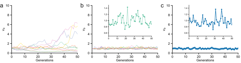
Figure 1: Cell size at birth in simulations (a,b) and in experiments (c) as a discrete time-series, with insets showing a zoomed in view of one particular trial of simulation (b) and the data (c). (a,b) Multiple trials (different colors) of numerical simulations of the DSM in Eq. 9 with the simple, one-line pseudo-code: $v_{i+1}=\left(2\left(1-\alpha\right)v_{i}+v_{0}\right)2^{\xi_{t}}/2$, where $v_{i}$ denote cell size at birth in the $i$-th generation, $\xi_{t}$ is a normally distributed random variable with zero mean and variance $\sigma_{t}^{2}$, and $v_{0}$ is a constant that sets the mean cell size. Here, $\sigma_{t}=0.22$ and $\left\langle v_{b}\right\rangle=1$. (a) $\alpha=0$ leads to unconfined diffusion and a divergent distribution. (b) Any $0<\alpha<2$, here $\alpha=0.5$, has the necessary feedback to achieve a stationary distribution. (c) Data from Ref. youData . $v_{b}$ in this case represents cell length at birth and is normalized so that $\left\langle v_{b}\right\rangle=1$.

II.2 Approximate solution via first order expansion

The DSM described in Section II.1 is in general difficult to solve for an arbitrary size regulation strategy $f\left(v_{b}\right)$. One method makes the approximation to focus on the behavior of $f$ near the mean size $\left\langle v_{b}\right\rangle$, since the size distribution has a small CV. A size regulation strategy can be linearized by expanding about $\left\langle v_{b}\right\rangle$, $f\left(v_{b}\right)\approx f\left(\left\langle v_{b}\right\rangle\right)+f^{\prime}\left(\left\langle v_{b}\right\rangle\right)\left(v_{b}-\left\langle v_{b}\right\rangle\right).$ In this approximation, all regulation strategies that agree to first order will lead to similar distributions near $\left\langle v_{b}\right\rangle$. The following is a convenient choice amir ,

$$f\left(v_{b}\right)=2v_{b}^{1-\alpha}v_{0}^{\alpha},$$ (10)

where $v_{0}$ is an arbitrary constant. As shown below, $\left\langle v_{b}\right\rangle\approx v_{0}$, and hence, the slope has value $f^{\prime}\left(\left\langle v_{b}\right\rangle\right)=2\left(1-\alpha\right)$. The value of $\alpha$ therefore determines the strength of regulation. $\alpha=1$ corresponds to the strongest regulation, a “sizer” strategy where cells attempt to divide upon reaching $f\left(v_{b}\right)=2v_{0}$. $\alpha=0$ represents no regulation and corresponds to the timer strategy where cells attempt to divide upon reaching $f\left(v_{b}\right)=2v_{b}$. Recent works have shown that the statistics of cell size can be generated by a regulation strength $\alpha=1/2$ that is between the two extremes jun ; jw ; elf ; junReview . In this case, the slope has value $f^{\prime}\left(\left\langle v_{b}\right\rangle\right)=1$ and so is an approximation to the “adder” strategy (also known as the incremental model voorn ; koppes ) where cells attempt to divide upon reaching $f\left(v_{b}\right)=v_{b}+v_{0}$. Several microorganisms in all three domains of life have been shown to approximately follow an adder strategy, or less prescriptively, to exhibit adder correlations. We discuss the prevalence of adder correlations later.

Let $x=\ln\left(v_{b}/v_{0}\right)$ be the log-size and $x^{\prime}$ denote $x$ at the next generation. Eqs. 9-10 then lead to the simple stochastic equation

$$x^{\prime}=\left(1-\alpha\right)x+\lambda\xi_{t}.$$ (11)

At the $n$-th generation,

$$x_{n}=\left(1-\alpha\right)^{n}x_{0}+\sum_{j=0}^{n-1}\left(1-\alpha\right)^{n-1-j}\lambda\xi_{t}^{\left(j\right)},$$ (12)

where $x_{i}$ and $\xi_{t}^{\left(i\right)}$ respectively denote the value of $x$ and $\xi_{t}$ at the $i$-th generation. The first term approaches zero as $n\to\infty$ if $0<\alpha<2$. If $\xi_{t}$ is normally distributed with variance $\sigma_{t}^{2}$, then the variance $\sigma_{x}^{2}$ of $x$ will be the sum of the variances in the series in the second term. The geometric series converges for $0<\alpha<2$, and can readily be evaluated to give the variance $\sigma_{x}^{2}$ as

$$\sigma_{x}^{2}=\frac{\lambda^{2}\sigma_{t}^{2}}{\alpha\left(2-\alpha\right)}.$$ (13)

Furthermore, since $x_{n}$ is a sum of normal variables, it will also be normally distributed. If $\alpha\leq 0$ or $\alpha\geq 2$, the sum of the series diverges, and hence there is no stationary distribution. The case $\alpha=0$ produces unconfined diffusion and is analogous to the case where the strength of the restoring force is zero ($k=0$) in an OU process, as seen in Eq. 5. Fig. 1ab demonstrates the difference between time-series generated by $\alpha=0$ and by $0<\alpha<2$. The variance of $t_{d}$ can be obtained similarly.

It is not obvious a priori whether the widths of the distributions of interdivision time and cell size are related. It turns out that the two CVs (denoted by $CV\left(\cdot\right)$) are related by a dimensionless quantity amir . The log-size is related to the actual size by $x=\ln\left(v_{b}/v_{0}\right)\equiv\ln\left(1+\delta v_{b}\right)$. Since $\delta v_{b}=v_{b}/v_{0}-1$ is small, $x\approx\delta v_{b}=v_{b}/v_{0}-1$. Therefore, $CV\left(v_{b}\right)\approx\sigma_{x}$. Calculating $CV\left(t_{d}\right)$ in a similar manner leads to

$$\frac{CV\left(v_{b}\right)}{CV\left(t_{d}\right)}\approx\frac{\ln 2}{\sqrt{2\alpha}}.$$ (14)

Eq. 14 allows to extract the parameter $\alpha$ from CVs that can be accurately measured. Since $x$ and $t_{d}$ are both distributed normally, the model predicts that these distributions can be collapsed after normalizing by the mean and scaling according to Eq. 14, as seen in experiments jun ; soifer .

The Pearson correlation coefficients (CC) between two variables (denoted by $C\left(\cdot,\cdot\right)$) can also be obtained. Since CCs are not affected by addition or multiplication by a constant, $v_{b}$ can be replaced by $x$ in the following calculations. The CC between cell size at birth of a mother cell and that of the daughter cell is therefore amir

$$C\left(v_{b},v_{b}^{\prime}\right)=C\left(x,x^{\prime}\right)=\frac{\left\langle xx^{\prime}\right\rangle-\left\langle x\right\rangle^{2}}{\sigma_{x}^{2}}.$$ (15)

Substituting in Eq. 11,

$$C\left(v_{b},v_{b}^{\prime}\right)=1-\alpha.$$ (16)

Importantly, the value of $\alpha\approx 1/2$ extracted via the ratio of CVs in Eq. 14 also predicts the CC between size at birth and at division, in agreement with experiments jun ; jw ; koppes80 .

Similarly, using Eq. 8 and 10, the interdivision time can be written as

$$t_{d}=\frac{\ln 2-\alpha x}{\lambda}+\xi_{t}.$$ (17)

The CC between the interdivision times of a mother-daughter pair can then be shown to be jun ; lin

$$C\left(t_{d},t_{d}^{\prime}\right)=-\alpha/2.$$ (18)

That this CC is non-zero has implications for the population growth rate, which we review later.

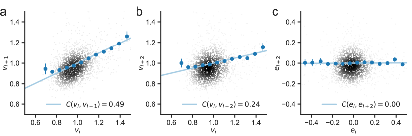
Figure 2: Cell size at birth in E. coli can be described by an AR(1) model. Data is the same as that in Fig. 1 youData . (a-b) Single-cell data of cell size at birth $v_{i}$ at the $i$-th generation and the resulting CCs between parent and children (a) and parent and grand-children (b). (c) The residuals $e_{i}$ after linear regression with $v_{i+1}$ and the resulting CC, $C\left(e_{i},e_{i+2}\right)$. See text for details. Gray dots show data, with color representing the density of points. Blue circles show average values binned according to values on the $x$-axis. Error bars show one SEM. Blue lines show the best linear regression of raw data.

II.3 Autoregressive models and extensions to incorporate biological details

Eq. 11, obtained after linearization of the generically nonlinear DSM Eq. 9, is mathematically known as an autoregressive (AR) model, often used in time-series analysis and economics forecasting priestley . An AR model of order $m$ (denoted by AR($m$)) takes the form $x_{i}=b+\sum_{j=1}^{m}c_{j}x_{i-j}+\xi_{i}$, where $b$ and $c_{j}$ are constants and $\xi_{i}$ is a noise term uncorrelated for different $i$. The model describes how previous values of the stochastic variable $x$ influence linearly the next value. Eq. 11 is an AR(1) model, which is also a discrete analogue of an OU process.

In the problem of cell size regulation, it is not obvious a priori if an AR(1) model is sufficient to describe data. One method to determine the appropriate order of an AR model is to investigate the partial correlation coefficients. The partial CC between $x_{i}$ and $x_{i+2}$ given an intermediate variable $x_{i+1}$ is defined as the CC between the residuals $e_{i}=x_{i}-\hat{x}_{i}$ and $e_{i+2}=x_{i+2}-\hat{x}_{i+2}$. $\hat{x}_{i}=p_{1}x_{i+1}+p_{0}$ and $\hat{x}_{i+2}=q_{1}x_{i+1}+q_{0}$ denote the predicted value after linear regression with $x_{i+1}$ to determine the coefficients. The resulting partial CC between $x_{i}$ and $x_{i+2}$, with the intermediate variable $x_{i+1}$, is priestley

$$\begin{split}C_{x_{i+1}}\left(x_{i},x_{i+2}\right)=C\left(e_{i},e_{i+2}\right)\\ =\frac{C\left(x_{i},x_{i+2}\right)-C\left(x_{i},x_{i+1}\right)C\left(x_{i+1},x_{i+2}\right)}{\sqrt{\left(1-C^{2}\left(x_{i},x_{i+1}\right)\right)\left(1-C^{2}\left(x_{i+1},x_{i+2}\right)\right)}}.\end{split}$$ (19)

In an AR(1) model, the CC $C\left(x_{i},x_{i+2}\right)$ is non-zero because they are related via the intermediate variable $x_{i+1}$. However, the partial CC $C_{x_{i+1}}\left(x_{i},x_{i+2}\right)$ removes the effects of the intermediate variable and is zero. Experimentally determined values of $C\left(v_{i},v_{i+1}\right)$ is as predicted by Eq. 16 (Fig. 2a) youData . In the same data set, $C\left(v_{i},v_{i+2}\right)$ is non-zero but $C_{v_{i+1}}\left(v_{i},v_{i+2}\right)$ is zero (Fig. 2bc). Indeed, a vanishing $C_{v_{i+1}}\left(v_{i},v_{i+2}\right)$ implies that $C\left(v_{i},v_{i+2}\right)=C^{2}\left(v_{i},v_{i+1}\right)$, which is the case here. This novel check systematically shows that cell size at birth in E. coli can be described by an AR(1) model. This result is a fortunate simplification, since for example, in certain mammalian cells, the CCs in the interdivision times between cousin cells ($C_{\textnormal{cc}}$) cannot be determined from those between sister cells ($C_{\textnormal{ss}}$) and between mother-daughter pairs ($C_{\textnormal{md}}$). Instead, experiments observe that $C_{\textnormal{cc}}>C_{\textnormal{md }}$, contrary to the expected relation $C_{\textnormal{cc}}=C_{\textnormal{md}}^{2}C_{\textnormal{ss}}$ in an AR(1) model balaban ; balaban2 .

Extracting the regulation strength $\alpha$ via Eq. 16 is analogous to estimating the parameters in AR models via the Yule-Walker equations that relate theoretical values of the parameters to theoretical values of the autocorrelation function (ACF) priestley . The ACF $\rho\left(t\right)$ is the CC between variables separated by $t$ time points,

$$\rho\left(t\right)=C\left(x_{i},x_{i+t}\right).$$ (20)

As can be seen by Eq. 12, the ACF for the AR(1) model of Eq. 11 is simply

$$\rho\left(t\right)=\left(1-\alpha\right)^{\left|t\right|}.$$ (21)

In this case, the ACF decays exponentially as in an OU process as seen in Eq. 6. The ACF of cell size at birth indeed decays exponentially (Fig. 3a) you . Importantly, the estimated ACF is only meaningful after sufficient averaging to eliminate spurious fluctuations. This can be done most clearly by computing the power spectral density (PSD)

$$S\left(f\right)=\lim_{T\to\infty}\frac{1}{T}\left|\sum_{j=1}^{T}x_{j}e^{-i2\pi fj}\right|^{2},$$ (22)

where $T$ is the total number of observations in the time-series with data points $x_{j}$. The PSD can also be calculated as the Fourier transform of the ACF according to the Wiener-Khinchin theorem. For the AR(1) model of Eq. 11, the PSD turns out to be priestley

$$S\left(f\right)=\frac{\alpha\left(2-\alpha\right)}{1-2\left(1-\alpha\right)\cos\left(2\pi f\right)+\left(1-\alpha\right)^{2}}\sigma_{x}^{2}.$$ (23)

This is again analogous to an OU process, since the Fourier transform of an exponential function is a Lorentzian function. There are significant oscillations only in the case $\alpha\lesssim 2$, for which the PSD peaks at high frequencies (Fig. 3cd). The case of E. coli, where $\alpha\approx 1/2$, is far from this regime (Fig. 3ab). Therefore, experimentally observed fluctuations should not be confused for oscillations you .

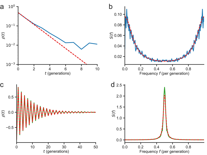
Figure 3: Fluctuations versus oscillations. The ACF $\rho\left(t\right)$ (a,c) and the PSD $S\left(f\right)$ (estimated via the Welch method) (b,d) of cell size at birth in E. coli (a,b) and a simulated AR(1) model described by Eq. 11 with $\alpha=1.9$ (c,d). Blue lines show experimentally determined ACF and PSD from the same data set as that in Fig. 1 youData . Green lines show simulation results. Dashed red lines show Eq. 21 (a,c) and Eq. 23 (b,d), for $\alpha=0.49$ (a,b) and $\alpha=1.9$ (c,d).

The AR(1) model in Eq. 11 can be extended to incorporate details that are relevant to a variety of microorganisms. These include asymmetric and noisy divisions (e.g. in mycobacteria aldridge ; logsdon ), noisy growth rates (e.g. in slow growing E. coli elf and in the archaeon H. salinarum eun ), and diverse growth morphologies (e.g. the budding mode of growth of S. cerevisiae soifer ). First, noisy divisions and noisy growth rates can be incorporated by modeling the division ratio (daughter cell size at birth divided by mother cell size at division) and growth rate as $1/2+\xi_{r}$ and $\lambda+\xi_{\lambda}$, respectively, at each generation. If the fluctuations $\xi_{r}$ and $\xi_{\lambda}$ are small and uncorrelated, Eq. 11 becomes to first order in small variables

$$x^{\prime}\approx\left(1-\alpha\right)x+\lambda\xi_{t}+2\xi_{r}.$$ (24)

The fluctuation $\xi_{\lambda}$ enters as a first order correction to interdivision time $t_{d}$. The CVs and CCs can be calculated as before for Eq. 24 to show that the different fluctuations typically affect the CVs and CCs in different ways. For example, the CC between cell size at birth and at division, $C\left(v_{b},v_{d}\right)$, is sensitive to fluctuations in division ratios, and is increased by large fluctuations in division ratios. However, the CC in cell size at birth between mother-daughter pairs, $C\left(v_{b},v_{b}^{\prime}\right)$, remains the same as in Eq. 16, and is independent of all noise terms. It is thus a robust detector of the underlying regulation strategy even in face of multiple sources of complicating stochasticity eun . We discuss later several models that incorporate other biological details and move beyond AR models.

II.4 Continuous rate models and higher order effects

Cell size regulation can also be modeled using continuous rate models (CRM) jun ; lagomarsinoPRE16 ; lagomarsinoPRE17 ; lagomarsinoConcerted . In contrast to DSMs, CRMs consider not just discrete division events, but the continuous cell cycle. They specify the instantaneous division rate $h$, or the probability to divide per unit size increment, as a function of physiological parameters such as the current size $v$, size at birth $v_{b}$, growth rate $\lambda$, or the time $t$ since division. A simple choice of parametrization is the sloppy sizer model, $h=h\left(v\right)$. In this case, the probability for a cell of size $v$ to divide between the size interval $v$ and $v+dv$ is $h\left(v\right)dv$. Hence if $F\left(v_{d}|v_{b}\right)$ is the cumulative probability to have not divided at size $v_{d}$ given $v_{b}$, then $F\left(v_{d}|v_{b}\right)$ satisfies $F\left(v_{d}+dv|v_{b}\right)=F\left(v_{d}|v_{b}\right)\left(1-h\left(v_{d}\right)dv\right)$. In the continuum limit, $dF\left(v_{d}|v_{b}\right)/dv=-h\left(v_{d}\right)F\left(v_{d}|v_{b}\right)$, so that

$$F\left(v_{d}|v_{b}\right)=\exp\left(-\int_{v_{b}}^{v_{d}}h\left(v\right)dv\right).$$ (25)

Eq. 25 can be written as

$$h\left(v\right)=-\frac{d}{dv}\ln F\left(v|v_{b}\right),$$ (26)

allowing to extract $h\left(v\right)$ via single-cell experiments that measure $F\left(v_{d}|v_{b}\right)$. The division rate can be formulated as a probability to divide per unit time increment as well, using the change of variables between size and time given by exponential growth. Analyses using CRMs have demonstrated that the current size is not the only determinant of the division rate because the sloppy sizer model fails to capture measured distributions of interdivision time and size increment from birth to division lagomarsinoConcerted . This implies that there exists a feedback on the time since birth, or equivalently the size at birth lagomarsinoConcerted . Specifically, a division rate in the form $h=h\left(v-v_{b}\right)$ can simultaneously describe measured distributions of size at birth, interdivision time, and size increment from birth to division jun .

A CRM can be approximately reduced to a DSM with the target size at division equal to the expectation value of the size at division given the size at birth lagomarsinoPRE17 ,

$$f\left(v_{b}\right)=\int_{0}^{\infty}p\left(v|v_{b}\right)vdv,$$ (27)

where $p\left(v|v_{b}\right)=-dF\left(v|v_{b}\right)/dv$ is the probability density for a cell born at size $v_{b}$ to divide at size $v$. The nature and magnitude of the noise term can be determined by inverting the steps described below to map a DSM to a corresponding CRM. To do so, $p\left(v|v_{b}\right)$ can be calculated from $f\left(v_{b}\right)$ and a specified coarse-grained noise, then the division rate can be obtained using Eq. 26. For example, for a time-additive, normally distributed noise with variance $\sigma_{t}^{2}$, the division probability density for log-size $x=\ln\left(v/v_{0}\right)$ is $p\left(x|x_{b}\right)\propto\exp\left(-\left(x-g\left(x_{b}\right)\right)^{2}/\left(2\lambda^{2}\sigma_{t}^{2}\right)\right)$, where $g\left(x_{b}\right)=\ln\left(f\left(v_{0}e^{x_{b}}\right)/v_{0}\right)$. Since the typical $x_{b}$ is much smaller than $g\left(x_{b}\right)$, integration leads to the division rate lagomarsinoPRE17

$$h\left(v,v_{b}\right)\approx\frac{\sqrt{2}}{v\sqrt{\pi}\lambda\sigma_{t}}H\left(\frac{1}{\sqrt{2}\lambda\sigma_{t}}\ln\left(\frac{v}{f\left(v_{b}\right)}\right)\right),$$ (28)

where $H\left(z\right)=\exp\left(-z^{2}\right)/\left(1-\textnormal{Erf}\left(z\right)\right)$ and $\textnormal{Erf}\left(\cdot\right)$ is the error function. For the regulatory function Eq. 10, the division rate Eq. 28 becomes a function of only the instantaneous size when $\alpha=1$, corresponding to a sizer strategy.

Although the CRM is generic and may capture complex behavior such as filamentation lagomarsinoConcerted , it is not obvious a priori how to parametrize the division rate. On the other hand, the DSM has only a few parameters, is amenable to analytical treatment in several cases, and describes existing measurements well. The complexity sacrificed by DSMs and their first order approximate solutions may become important, for instance, when second and higher order terms become significant. However, higher order effects are difficult to detect unless the number of cells measured is large enough to suppress the confounding effects of fluctuations in the cell cycle. No existing experiments have achieved this regime, perhaps justifying the success of DSMs as models of cell size regulation lagomarsinoPRE17 .

II.5 More precise analyses of DSMs

The approximate first order solution in Section II.2 predicts a log-normal size distribution for a regulatory function $f\left(v_{b}\right)=2\left(1-\alpha\right)v_{b}+v_{0}$ and a time-additive, normally distributed noise. However, closer inspection reveals that the size distribution has a power-law tail instead. This can be seen by analyzing which moments exist for a given regulation strength $\alpha$. Calculations similar to those in Section II.2 show that if the $j$-th moment exists, so too do all the lower moments, but that for any $\alpha>0$, there always exists an integer $j^{*}$ past which all moments cease to exist. This suggests that the size distribution has a power-law tail $p\left(v_{b}\right)\sim 1/v_{b}^{1+\beta}$ with $j^{*}<\beta\leq j^{*}+1$, as confirmed by numerical simulations marantan .

The value of $\beta$ can be obtained precisely. The evolution of size distributions from one generation to the next can be written as an integral equation $p\left(v^{\prime}_{b}\right)=\int_{0}^{\infty}K\left(v^{\prime}_{b},v_{b}\right)p\left(v_{b}\right)dv_{b},$ where the kernel $K\left(v_{b}^{\prime},v_{b}\right)$ can be derived from the regulatory strategy $f\left(v_{b}\right)$. For a regulatory function in the form $f\left(v_{b}\right)=2\left(1-\alpha\right)v_{0}\left(v_{b}/v_{0}\right)^{\eta}+v_{0}$, it can be shown via an asymptotic analysis of the integral equation that a distribution with a power-law tail $1/v_{b}^{1+\beta}$ evolves to one with a power-law tail $1/v_{b}^{1+\beta/\eta^{2}}$ marantan . This implies that for $\eta=1$, the stable size distribution indeed has a power-law tail, with

$$\beta=\frac{-2\ln\left(1-\alpha\right)}{\lambda^{2}\sigma_{t}^{2}},$$ (29)

where $\sigma_{t}^{2}$ is the variance of the time-additive noise.

An alternative approach also led to the same power-law tail burov . In this approach, a DSM is approximated as a Langevin equation continuous in generations. Let $x=\ln\left(v_{b}/v_{0}\right)$ be the log-size at birth and let $n$ denote the generation number, then Eq. 9 can be written

$$x_{n+1}=x_{n}+\tilde{g}\left(x_{n}\right)+\lambda\xi_{t},$$ (30)

where $\tilde{g}\left(x_{n}\right)=\ln\left(f\left(\exp\left(x_{n}\right)v_{0}\right)/v_{0}\right)-x_{n}$. To lowest order, Eq. 30 can be approximated by a Langevin equation continuous in $n$ as

$$\frac{dx}{dn}=\tilde{g}\left(x\right)+\lambda\xi_{t}.$$ (31)

As seen before in the context of an OU process described by Eq. 3, Eq. 31 leads to an equilibrium distribution of log-sizes $p\left(x\right)\propto\exp\left(-2V\left(x\right)/\left(\lambda^{2}\sigma_{t}^{2}\right)\right)$, where $V\left(x\right)=\int\tilde{g}\left(x^{\prime}\right)dx^{\prime}$ is the effective potential. For the same regulatory function as above, the effective potential diverges linearly as $V\left(x\right)\sim-2x\ln\left(1-\alpha\right)$. The equilibrium distribution therefore has a power-law tail $1/v_{b}^{1+\beta}$ with the same $\beta$ as in Eq. 29 burov . Even further precision can be obtained via a second order approximation which modifies the effective potential, but leaves the behavior of the power-tail unchanged burov .

III Beyond phenomenological models of cell size regulation

As we previously alluded, the formalism of DSMs developed for the problem of cell size regulation can lead to insights on related problems at the molecular, single-cell, and the population level. Below, we discuss these in turn.

III.1 Molecular mechanisms to implement cell size regulation

How does a bacterial cell molecularly implement a size regulation strategy? The initiator accumulation model is a network architecture proposing that an initiator protein accumulates during cell growth to trigger cell division upon reaching a threshold copy number $\theta$ sompayrac . While experiments have suggested that the upstream control occurs over initiation of DNA replication rather than cell division in various microorganisms donachie ; liu ; soifer ; amirSpandrel , we first review a simpler model where the accumulation of initiators triggers cell division. The model leads to the adder correlations observed in several species of bacteria and other microorganisms barber ; amir ; ho .

One possible molecular implementation of the initiator accumulation model is as follows singh . If the transcription rate of the initiator is assumed to be proportional to the cell volume, which grows exponentially in time, and if each transcript leads to a burst of protein production with mean burst size $b$, then the distribution of added cell size $\Delta v=v_{d}-v_{b}$ from birth to division has width singh

$$CV^{2}\left(\Delta v\right)=\frac{b^{2}+2b\theta+\theta}{\left(b+\theta\right)^{2}}.$$ (32)

Furthermore, the resulting distribution has only one characteristic size, the mean added cell size $\left\langle\Delta v\right\rangle$, and therefore can be written as

$$p\left(\Delta v\right)=\frac{1}{\left\langle\Delta v\right\rangle}\tilde{p}\left(\frac{\Delta v}{\left\langle\Delta v\right\rangle}\right).$$ (33)

Indeed, experiments showed that distributions of cell sizes with different means collapse after normalizing by the mean jun ; lagomarsinoPRE16 ; woldringh ; giometto . The collapse suggests that $b$ and $\theta$ are constant within the implementation here. The same experiments also saw that the distributions of interdivision times collapse after normalizing by the mean doubling time, which is again captured by this model singh . There are also additional models that show such scaling collapse, such as an autocatalytic network subject to a threshold criterion for division iyerbiswas , and the coarse-grained “adder-per-origin” model described below.

As discussed in the Introduction, control at other cell cycle events may lie upstream of cell division in various microorganisms. DSMs similar to those reviewed so far can be extended to describe cell cycle regulation. These models can not only produce emergent strategies of cell size regulation identical to those described by the division-centric models reviewed so far, but also describe additional statistics such as the correlations between cell size and various cell cycle timings lagomarsinoTrends ; adicipt .

As an example, we review below a model of cell cycle regulation in E. coli, whose cell divisions appear to follow a constant time $T$ after the initiation of DNA replication for a broad range of mean growth rates huang ; ch . The time $T$ can be larger than the mean doubling time $\tau$, in which case the cells maintain multiple ongoing rounds of DNA replication. The tight coupling between initiation and division implies that the cell size at birth $v_{d}$ is

$$v_{d}=v_{i}e^{\lambda\left(T+\xi_{T}\right)},$$ (34)

where $v_{i}$ is the cell size at initiation, $\lambda=\ln 2/\tau$ is the growth rate, and $\xi_{T}$ describes fluctuations with magnitude $\sigma_{T}$ in the time between initiation and division. At a coarse-grained level, the initiator accumulation model can be described as sompayrac ; amir ; ho

$$\tilde{v}_{i}^{\prime}=\left(v_{i}+Ov_{0}\right)e^{\lambda\xi_{t}},$$ (35)

where $\tilde{v}_{i}^{\prime}$ is the total cell size of the daughter cells (typically two) at the next initiation, $O$ is the number of origins of replication (i.e. the site along the chromosome at which DNA replication initiates), and $v_{0}$ is a constant. As in the division-centric model, regulation is subject to a time-additive noise $\xi_{t}$ with magnitude $\sigma_{t}$.

Analysis and simulations of the initiation-centric model of Eqs. 34-35 show that it produces emergent adder correlations at division ho ; barber , as long as the magnitude of the fluctuations in the coordination between initiation and division is much less than that in the control of initiation ($\sigma_{t}\gg\sigma_{T}$). This is indeed the case in experiments for fast-growing bacteria, although the picture appears different for slow-growing bacteria elf , which we discuss later. The model also generates cell size and interdivision time distributions whose CVs only depend on the magnitudes $\lambda\sigma_{t}$ and $\lambda\sigma_{T}$ of the fluctuations, and the regulation strength $\alpha$. The distributions therefore collapse after scaling by the mean if these parameters are constant across growth conditions. At the bulk-level, the initiation-centric model produces the observed exponential scaling of mean cell size with mean growth rate, as discussed in the Introduction, without requiring parameters to depend on mean growth rate ho . These results, together with previous results regarding the universality of cell size distributions, suggest that the initiator accumulation model may be a robust molecular mechanism that produces adder correlations, and that models of cell cycle regulation can continue to shed light on the underlying biology.

III.2 Regulation of protein numbers

Recent works have begun investigating the statistics of the copy numbers of proteins at the single-cell level in the same spirit as the problem of cell size regulation you ; brennerEPJE ; brennerPRE ; brennerMulticomp . In fact, for a constitutively expressed protein, the distributions of protein numbers at birth can be described by a DSM brennerPRE . Analysis analogous to that in Fig. 2, but for the copy number of a constitutively expressed protein in E. coli in the same data set youData , reveals that the partial CC is also zero in this case. However, it is unclear how protein number and cell size are simultaneously regulated.

One way to investigate this question is via a multi-dimensional, or vector, AR model. An AR(1) vector model in $M$ dimensions can be written as

$$\vec{x}^{\prime}=A\vec{x}+\vec{b}+\vec{\xi},$$ (36)

where $\vec{x}$ is a vector of the abundances at birth of the $M$ cellular components, which can include cell size, and $\vec{x}^{\prime}$ is the vector at the next generation. $A$ is a $M\times M$ matrix representing the regulatory interactions between components, $\vec{b}$ is a vector representing the basal synthesis level between generations, and $\vec{\xi}$ is a vector of noise terms uncorrelated between generations but may be cross-correlated at the same generation.

For the one-dimensional case, the condition for stationarity is that $2>\alpha>0$ so that the variance of $x$ in Eq. 13 is finite. This condition is equivalent to that the zero of $1-\left(1-\alpha\right)z$ lie outside the unit circle. In the multi-dimensional case, the condition is similarly that all the zeros of $\det\left(I-Az\right)$ lie outside the unit circle priestley . Given a stable AR(1) vector model, the multi-dimensional analogue of the Yule-Walker equations can be used to estimate by maximum likelihood the regulatory matrix $A$ from measurements box . For the data set discussed above youData , this method results in

$$A=\left(\begin{array}[]{cc}0.50\pm 0.02&-0.02\pm 0.01\\ -0.16\pm 0.02&0.60\pm 0.02\end{array}\right),$$

where the first and second components are respectively cell size and protein number at birth (both normalized by their means), and plus-minus shows the standard error in the estimate. This novel result suggests that the copy number of this constitutively expressed protein does not affect cell size regulation, while cell size does affect the regulation of this protein number. It is unknown whether this result holds for all constitutively expressed proteins, and how this result will change for proteins that are not constitutively expressed.

To better understand cross-correlations between cell size and protein numbers from a mechanistic perspective, recent works have investigated a dynamical model in the form $d\vec{x}/dt=A\vec{x}$, where $\vec{x}$ is now the abundances of the cellular components during the cell cycle, and $A$ now describes the regulatory interactions in time brennerMulticomp . This model leads to the components growing as a sum of exponentials that can be approximated as a single exponential function during one generation, in agreement with experimentally observed exponential growth brennerEPJE . Describing the statistics generated by dynamical models, and relating a dynamical model to a DSM and vice versa remain important open questions.

III.3 Effects of cell size regulation on population growth rate

At the single-cell level, genetically identical cells in the same clonal populations may have different interdivision times and growth rates. How does such variability at the single-cell level affect population growth? Models often assume that the interdivision times $t_{d}$ are uncorrelated between generations and independent of other variables powell ; hashimoto ; iyerbiswasPop . In this case, a simple relation connects the asymptotic population growth rate $\Lambda=\left(dN/dt\right)/N$, where $N$ is the number of cells in the population, to the interdivision time distribution $p\left(t_{d}\right)$,

$$2\int_{0}^{\infty}p\left(t_{d}\right)\exp\left(-\Lambda t_{d}\right)=1.$$ (37)

Importantly, given a fixed mean interdivision time, a larger variability in $t_{d}$ increases $\Lambda$. However, cell size regulation leads to negative correlations in $t_{d}$ between generations, as seen in Eq. 18. In this case, recent results obtained by some of us showed that in an asynchronous, exponentially growing population - in which each cell is subject to variability in its single-cell growth rate, as well as to time-additive and size-additive noise in its cell size regulation by the regulatory function $f\left(v_{b}\right)=2\left(1-\alpha\right)v_{b}+2\alpha v_{0}$ - the population growth rate is dependent only on the distribution of single-cell growth rates. In the limit of small correlations in growth rates between generations, variability in single-cell growth rates does not increase, but rather decreases the population growth rate lin ,

$$\Lambda/\left\langle\lambda\right\rangle=1-\left(1-\frac{\ln 2}{2}\right)CV^{2}\left(\lambda\right),$$ (38)

Eq. 38 predicts that a population can enhance its population growth rate by suppressing the variability in single-cell growth rates given a fixed mean, which is consistent with the smaller CV of single-cell growth rates than that of interdivision times observed in experiments (Fig. 4ab) jun ; elf . Eq. 38 holds for any size regulation strategy $1>\alpha>0$, implying that cell size regulation, as long as it exists (in particular, $\alpha\neq 0$ leads instead to Eq. 37), does not affect population growth rate within the models studied here (Fig. 4a).

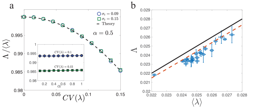
Figure 4: Cell size regulation, as long as it exists, does not affect population growth rate. (a) Population growth rates obtained from simulations (symbols) of an exponentially growing population subject to variability in single-cell growth rates agree with Eq. 38 (dashed line). Inset shows population growth rates do not vary with the regulation strength as long as $1>\alpha>0$. (b) Variability in single-cell growth rates decreases population growth rate. Blue squares show data from stewart (details of the error bars can be found in lin ). Red dashed line shows Eq. 38 for $CV\left(\lambda\right)$ measured by experiments. Black solid line shows $\Lambda=\left\langle\lambda\right\rangle$ as a guide. Both axes have units $\textnormal{min}^{-1}$. Adapted from lin .

IV Discussion

In this review, we summarized the mathematical formulations of the problem of cell size regulation, with a focus on coarse-grained, discrete models. As an example, we showed that a first order autoregressive model can describe the statistics of cell size in E. coli. We discussed how detailed analyses of such models led to several biologically relevant insights at the molecular, single-cell, and population level. The same approach may shed light on several outstanding questions.

First, the prevalence of adder correlations in all three domains of life (e.g. the prokaryote E. coli jun ; jw ; elf , the eukaryote S. cerevisiae soifer , and the archaeon H. salinarum eun ) suggest that it may be simpler to implement or may be evolutionarily advantageous compared to other size regulation strategies. An explanation of the prevalence of adder correlations remains missing, however, since cell size regulation was found not to affect population growth rate within the class of phenomenological growth models reviewed here lin .

In contrast, the mean single-cell growth rate affects cell size regulation, since E. coli in slow growth conditions no longer exhibits adder correlations elf . This observation may be explained by introducing stochasticity in single-cell growth rates into the initiation-centric model discussed in Section III.1, which can lead to a size regulation strategy that varies with mean growth rates elf . Indeed, cell size regulation may potentially be an emergent property of cell cycle regulation amirSpandrel . This view is further supported by several models that describe cell division as a downstream effect of another cell cycle event (e.g. initiation of DNA replication in M. smegmatis logsdon , the onset of budding in S. cerevisiae barber ; soifer , and septum constriction in C. crescentus dinner ), and nonetheless reproduces the observed statistics at divisions.

Models of cell size regulation may also incorporate diverse growth morphologies. For example in S. cerevisiae, division asymmetry depends on the duration of the budded phase, during which all cell growth occurs for the budded daughter cell soifer . In M. smegmatis, cell growth occurs at the two poles of the cell: the old pole grows faster than the new pole, and on average, the daughter that inherits the old pole is larger aldridge . In both cases, the subpopulations formed by the larger and smaller daughter cells exhibit different emergent size regulation strategies logsdon ; soifer . Models incorporating these details move beyond AR models but remain straightforward to simulate numerically, allowing the statistics they generate to be compared to experiments to distinguish between competing models.

At the molecular level, the behavior of molecular network architectures require further analysis. The particular implementation of an initiator accumulation model discussed in Section III.1 made the strong assumption that transcription rate is proportional to cell volume singh . It would be interesting to study more detailed network architectures, where this would be a result rather than a model assumption. Models at the molecular level may also begin to investigate the problem of protein number regulation. Since proteins are made by ribosomes, an important problem is how ribosomes are allocated towards translating different types of proteins. Quantitative patterns at the bulk level have emerged regarding ribosome allocation hwa ; barkai , but the picture at the dynamical, cell cycle level is less clear. Models of stochastic gene expression that extend existing ones, which often consider a fixed cell volume paulsson , to incorporate cell cycle regulation could shed light in this aspect.

Incorporating cell cycle regulation can in turn help understand cell size regulation in organisms with a circadian clock, such as mammalian cells and cyanobacteria. Recent works have begun to examine cell size regulation in these organisms balaban ; balaban2 ; huangCyano ; martins , and some have suggested that the circadian clock may affect cell size regulation in these organisms. How to model these processes at a molecular, coarse-grained, and population level remain intriguing questions.

IV.1 Which model should we use?

Since the various classes of models of cell size regulation reviewed here are quite different fundamentally, we conclude by discussing the question of which model to use to analyze what data or to elucidate what phenomenon. First, as discussed in Section II.4, continuous rate models (CRMs) differ from discrete stochastic maps (DSMs) in that CRMs take as parameter an entire function that describes the instantaneous division rate, whereas DSMs take, for example, only the strength of regulation and the magnitude of the coarse-grained stochasticity (although the form of the stochasticity must be assumed). Moreover, CRMs assume a priori whether regulation depends only on the current size or also on the size at birth, whereas DSMs can be used to determine the mode of regulation. These could be reasons for the increasing visibility of DSMs as models of cell size regulation.

Another fundamental distinction is the difference between division-centric models and models that place control at an upstream event. Division-centric models, such as those described by Eq. 9, makes the strong assumption that all information relevant for determining division timing is stored in the current size and the size at birth. This does not have to be the case. For example, it is widely accepted that in S. cerevisiae, control occurs over the Start transition and the duration of the budded phase is uncorrelated with size soifer . As reviewed briefly in Section III.1, Eq. 9 can be adapted to place control at various cell cycle events, which may then lead to additional predictions that can illuminate the coupling between different cell cycle events.

The above distinction does not imply that we should always use the most detailed description. To cite Levins, “All models leave out a lot and are in that sense false, incomplete, inadequate. The validation of a model is not that it is ’true’ but that it generates good testable hypotheses relevant to important problems levins .” It is often helpful to sacrifice details not pertinent to the phenomenon under consideration. For example, the initiator accumulation model can be considered to trigger division rather than initiation. Yet the simplified model may still provide mechanistic insights into the statistical properties, as discussed in Section III.1. These mechanistic models are altogether different from the phenomenological DSMs and CRMs.

In summary, the appropriate model to use depends not only on the organism or system in question, but also on the phenomena explored within the model. We have sketched here a map of the existing models. Technological advances now enable collection of more accurate and larger data sets. These will likely stimulate further development of models, which in turn will influence experimental directions.

Summary points

1. Studying quantitative patterns associated with cell size, and modeling them using stochastic models, can shed light on the underlying biological mechanisms.

2. Cell size in E. coli can be described by a first order autoregressive model in which the present value depends only on the value in the previous generation.

3. The initiator accumulation model is a molecular network architecture of cell size regulation that appears to be consistent with existing experimental results in bacteria.

4. Cell size regulation, as long as it is present, does not affect population growth rate within existing models.

Future issues

1. What is the reason for the prevalence of adder correlations for cell size regulation?

2. What are molecular implementations that regulate the cell cycle in changing environments, and what are the limits of biological stochasticity they can sustain?

3. How are the copy number of proteins and cell size simultaneously regulated, and how can the resulting statistics be described?

4. What are the couplings between cell size and cell cycle regulation to other cellular processes such as circadian clocks, and what models should we use to describe them?

References

- (1) A Koch. Bacterial growth and form. Springer, 2001.
- (2) L Willis and KC Huang. Sizing up the bacterial cell cycle. Nat. Rev. Microbiol., 15(10):606–20, 2017.
- (3) M Schaechter, O Maaloe, and NO Kjeldgaard. Dependency on medium and temperature of cell size and chemical composition during balanced growth of Salmonella typhimurium. J. Gen. Microbiol., 19:592–606, 1958.
- (4) NS Hill, R Kadoya, DK Chattoraj, and PA Levin. Cell size and the initiation of dna replication in bacteria. PLos Genet., 8(3):e1002549, 2012.
- (5) S Taheri-Araghi, S Bradde, JT Sauls, NS Hill, PA Levin, J Paulsson, M Vergassola, and S Jun. Cell-size control and homeostasis in bacteria. Curr. Biol., 25(3):385–91, 2015.
- (6) WD Donachie. Relationship between cell size and time of initiation of dna replication. Nature, 219(5158):1077–79, 1968.
- (7) L Harris and J Theriot. Relative rates of surface and volume synthesis set bacterial cell size. Cell, 165(6):1479–1492, 2016.
- (8) M Campos, IV Surotsev, S Kato, A Paintdakhi, B Beltran, SE Ebmeier, and C Jacobs-Wagner. A constant size extension drives bacterial cell size homeostasis. Cell, 159(6):1433–46, 2014.
- (9) H Zheng, P Ho, M Jiang, B Tang, W Liu, D Li, X Yu, NE Kleckner, A Amir, and C Liu. Interrogating the Escherichia coli cell cycle by cell dimension perturbations. Proc. Natl. Acad. Sci., 113(52):15000–5, 2016.
- (10) M Godin, FF Delgado, S Son, WH Grover, AK Bryan, A Tzur, P Jorgensen, K Payer, AD Grossman, MW Kirschner, and SR Manalis. Using buoyant mass to measure the growth of single cells. Nat. Methods, 7(5):387–90, 2010.
- (11) L Sompayrac and O Maaloe. Autorepressor model for control of dna replication. Nat. New. Biol., 241(109):133–5, 1973.
- (12) PA Fantes. Control of cell size and cycle time in Schizosaccharomyces pombe. J. Cell. Sci., 24:51–67, 1977.
- (13) F Barber, P Ho, A Murray, and A Amir. Details matter: noise and model structure set the relationship between cell size and cell cycle timing. Front. Cell Dev. Biol., in press.
- (14) A Marantan and A Amir. Stochastic modeling of cell growth with symmetric or asymmetric division. Phys. Rev. E, 94:012405, 2016.
- (15) GEP Box, JS Hunter, and WG Hunter. Statistics for Experimenters. John Wiley and Sons, 2005.
- (16) C Gardiner. Stochastic methods: A handbook for the natural and social sciences. Springer, 2009.
- (17) Y Tanouchi, A Pai, H Park, S Huang, NE Buchler, and L You. Long-term growth data of Escherichia coli at a single-cell level. Sci Data, 4:170036, 2017.
- (18) P Wang, L Robert, J Pelletier, WL Dang, F Taddei, A Wright, and S Jun. Robust growth of Escherichia coli. Curr. Biol., 20(12):1099–103, 2010.
- (19) S Taheri-Araghi, SD Brown, JT Sauls, DB McIntosh, and S Jun. Single-cell physiology. Annu. Rev. Biophys., 44:123–42, 2015.
- (20) A Amir. Cell size regulation in bacteria. Phys. Rev. Lett., 112(20):208102, 2014.
- (21) M Wallden, D Fange, EG Lundius, O Baltekin, and J Elf. The synchronization of replication and division cycles in individual E. coli cells. Cell, 166(3):729–39, 2016.
- (22) JT Sauls, D Li, and S Jun. Adder and a coarse-grained approach to cell size homeostasis in bacteria. Curr. Opin. Cell Biol., 38:38–44, 2016.
- (23) WJ Voorn, LJ Koppes, and NB Grover. Mathematics of cell division in Escherichia coli: comparison between sloppy-size and incremental-size kinetics. Curr. Top. Mol. Gen., 1:187–194, 1993.
- (24) WJ Voorn and LJ Koppes. Skew or third moment of bacterial generation times. Arch. Microbiol., 169(1):43–51, 1997.
- (25) I Soifer, L Robert, and A Amir. Single-cell analysis of growth in budding yeast and bacteria reveals a common size regulation strategy. Curr. Biol., 26(3):356–361, 2016.
- (26) LJ Koppes, M Meyer, HB Oonk, MA de Jong, and N Nanninga. Correlation between size and age at different events in the cell division cycle of Escherichia coli. J. Bacteriol., 143(3):1241–52, 1980.
- (27) J Lin and A Amir. The effects of stochasticity at the single-cell level and cell size control on the population growth. Cell Systems, 5:1–10, 2017.
- (28) MB Priestley. Spectral analysis and time series. Academic Press, 1981.
- (29) O Sandler, S Pearl-Mizrahi, N Weiss, O Agam, I Simon, and NQ Balaban. Lineage correlations of single cell division time as a probe of cell-cycle dynamics. Nature, 519(7544):468–71, 2015.
- (30) N Mosheiff, BMC Martins, S Pearl-Mizrahi, A Gruenberger, S Helfrich, I Mihalcescu, D Kohlheyer, JCW Locke, L Glass, and NQ Balaban. Correlations of single-cell division times with and without periodic forcing. arXiv, page 1710.00349, 2017.
- (31) Y Tanouchi, A Pai, H Park, S Huang, R Stamatov, N Buchler, and L You. A noisy linear map underlies oscillations in cell size and gene expression in bacteria. Nature, 523(7560):357–60, 2015.
- (32) BB Aldridge, M Fernandez-Suarez, D Heller, V Ambravaneswaran, D Irimia, M Toner, and SM Fortune. Asymmetry and aging of mycobacterial cells lead to variable growth and antibiotic susceptibility. Science, 335(6064):100–4, 2012.
- (33) MM Logsdon, P Ho, K Papavinasasundaram, M Cokol, K Richardson, CM Sassetti, A Amir, and BB Aldridge. Coordination of cell cycle progression in mycobacteria. Curr. Biol., in press.
- (34) Y Eun, P Ho, M Kim, L Renner, S LaRussa, L Robert, A Schmid, E Garner, and A Amir. Archaeal cells share common size control with bacteria despite noisier growth and division. under review.
- (35) AS Kennard, M Osella, A Javer, J Grilli, P Nghe, S Tans, P Cicuta, and MC Lagomarsino. Individuality and universality in the growth-division laws of single E. coli cells. Phys. Rev. E, 93:012408, 2016.
- (36) J Grilli, M Osella, AS Kennard, and MC Lagomarsino. Relevant parameters in models of cell division control. Phys. Rev. E, 95(3):032411, 2017.
- (37) M Osella, E Nugent, and MC Lagomarsino. Concerted control of Escherichia coli cell division. Proc. Natl. Acad. Sci., 111(9):3431–5, 2014.
- (38) DA Kessler and S Burov. Effective potential for cellular size control. arXiv, page 1701.01725, 2017.
- (39) A Amir. Is cell size a spandrel? eLife, 6:e22186, 2017.
- (40) P Ho and A Amir. Simultaneous regulation of cell size and chromosome replication in bacteria. Front. Microbiol., 6:662, 2015.
- (41) KR Ghusinga, C Vargas-Garcia, and A Singh. A mechanistic stochastic framework for regulating bacterial cell division. Sci. Rep., 6:30229, 2016.
- (42) FJ Trueba, OM Neijssel, and CL Woldringh. Generality of the growth kinetics of the average individual cell in different bacterial populations. J. Bacteriol., 150(3):1048–55, 1982.
- (43) A Giometto, F Altermatt, F Carrara, A Maritan, and A Rinaldo. Scaling body size fluctuations. Proc. Natl. Acad. Sci., 110(12):4646–50, 2012.
- (44) S Iyer-Biswas, GE Crooks, NF Scherer, and AR Dinner. Universality in stochastic exponential growth. Phys. Rev. Lett., 113:028101, 2014.
- (45) M Osella, SJ Tans, and MC Lagomarsino. Step by step, cell by cell: quantification of the bacterial cell cycle. Trends. Microbiol., 25(4):250–6, 2017.
- (46) A Adiciptaningrum, M Osella, MC Moolman, MC Lagomarsino, and S Tans. Stochasticity and homeostasis in the E. coli replication and division cycle. Sci. Rep., 5:18261, 2015.
- (47) S Cooper and CE Helmstetter. Chromosome replication and the division cycle of Escherichia coli b/r. J. Mol. Biol., 31(3):519–40, 1968.
- (48) N Brenner, E Braun, A Yoney, L Susman, J Rotella, and H Salman. Single-cell protein dynamics reproduce universal fluctuations in cell populations. Eur. Phys. J. E, 38:102, 2015.
- (49) N Brenner, CM Newman, D Osmanovic, Y Rabin, H Salman, and DL Stein. Universal protein distributions in a model of cell growth and division. Phys. Rev. E, 92(4):042713, 2015.
- (50) L Susman, M Kohram, H Vashistha, JT Nechleba, H Salman, and N Brenner. Statistical properties and dynamics of phenotype components in individual bacteria. arXiv, page 1609.05513, 2017.
- (51) GEP Box, GM Jenkins, and GC Reinsel. Time series analysis: Forecasting and control. Prentice Hall, 1994.
- (52) EO Powell. Growth rate and generation time of bacteria, with special reference to continuous culture. J. Gen. Microbiol., 15:492–511, 1956.
- (53) M Hashimoto, T Nozoe, H Nakaoka, R Okura, S Akiyoshi, K Kaneko, E Kussell, and Y Wakamoto. Noise-driven growth rate gain in clonal cellular populations. Proc. Natl. Acad. Sci., 113(12):3251–6, 2016.
- (54) S Iyer-Biswas, H Gudjonson, CS Wright, J Riebling, E Dawson, K Lo, A Fiebig, S Crosson, and AR Dinner. Bridging the time scales of single-cell and population dynamics. arXiv, page 1611.05149, 2016.
- (55) EJ Stewart, R Madden, G Paul, and F Taddei. Aging and death in an organism that reproduces by morphologically symmetric division. PLoS Biol., 3(2):e45, 2005.
- (56) S Banerjee, K Lo, MK Daddysman, A Selewa, T Kuntz, AR Dinner, and NF Scherer. Biphasic growth dynamics control cell division in Caulobacter crescentus. Nat. Microbiol., 2:17116, 2017.
- (57) M Scott, CW Gunderson, EM Mateescu, Z Zhang, and T Hwa. Interdependence of cell growth and gene expression: origins and consequences. Science, 330(6007):1099–102, 2010.
- (58) E Metzl-Raz, M Kafri, G Yaakov, I Soifer, Y Gurvich, and N Barkai. Principles of cellular resource allocation revealed by condition-dependent proteome profiling. eLife, 6:e28034, 2017.
- (59) J Paulsson. Models of stochastic gene expression. Phys. Life Rev., 2:157–175, 2005.
- (60) FB Yu, L Willis, RMW Chau, A Zambon, M Horowitz, D Bhaya, KC Huang, and SR Quake. Long-term microfluidic tracking of coccoid cyanobacterial cells reveals robust control of division timing. BMC Biol., 15:11, 2017.
- (61) BMC Martins, AK Tooke, P Thomas, and JCW Locke. Cell size control driven by the circadian clock and environment in cyanobacteria. bioRxiv, page 183558, 2017.
- (62) R Levins. The strategy of model building in population biology. Amer. Sci., 54(4):421–31, 1966.