Optical Control of Exchange Interaction and Kondo Temperature in cold Atom Gas

Abstract

The relevance of magnetic impurity problems in cold atom systems depends crucially on the nature of the exchange interaction between itinerant fermionic atoms and localized impurity atoms. In particular, Kondo physics occurs only if the exchange interaction is anti-ferromagnetic, and strong enough to yield high enough Kondo temperature ($T_{K}/T_{F}\geq 0.1$). Focusing, as an example, on the experimentally accessible system of ultra-cold ¹⁷³Yb atoms, it is shown that the sign and strength of an exchange interaction between an itinerant Yb(¹S₀) atom and a trapped Yb(³P₀) atom can be optically controlled. Explicitly, as the light intensity increases (from zero), the exchange interaction changes from ferromagnetic to anti-ferromagnetic. When the light intensity is such that the system approaches a singlet Feshbach resonance (from below), the singlet scattering length $a_{S}$ is large and negative, and the Kondo temperature increases sharply.

Introduction: Controlling interaction between cold atoms is a godsend, as it turns atomic systems capable of demonstrating new phenomena that cannot be otherwise accessed within solid state physics proper exch-PRL-09 ; exch-RevModPhys-13 ; exch-Nature-98 ; exch-PRL-15 ; exch-RevModPhys-10 . In a series of theoretical laser-exch-PRL-96 ; laser-control-exch-PRL-2003 ; opt-tune-scatt-length-PRA-05 ; opt-Feshbach-PRA-2006 and experimental Feshbach-RevModPhys-2006 ; laser-exch-PRL04 ; laser-exch-PRA97 ; laser-exch-PRL11 ; laser-exch-Bachelors-2009 ; opt-Feshbach-prl-11 ; laser-exch-Science-2008 investigations, it has been established that, as far as potential scattering is concerned, the strength of atomic interactions can be tuned by laser beams. The prime object of these studies is to achieve an optical Feshbach resonance and thereby to obtain a Bose-Einstein condensate in cold bosonic atom systems.

On the other hand, the feasibility of controlling the strength and the sign of exchange interaction between atoms is much less studied. Its importance has been recognized recently, in the quest for studying the Kondo effect Hewson-book in cold atom systems Bauer . The physics exposed in the study of magnetic impurities when the itinerant (fermionic) atoms have spin $F\geq\frac{3}{2}$ is very rich, touching upon exotic phenomena such as over-screening KKAK-prb-15 , realization of the Coqblin-Schrieffer model IK-TK-YA-GBJ-PRB-16 , multipolar Kondo effect IK-TK-YA-GBJ-PRB-18 and others. Recently, it has been shown that exchange interaction can be controlled by the technique of confined-induced-resonance (CIR) CIR1 ; CIR2 ; CIR3 ; CIR4 .

The goal of the present study is to show that exchange interaction between fermionic atoms can be optically controlled . As an experimentally feasible example we consider ¹⁷³Yb atoms. Those in the ground state ¹S₀ are itinerant, (forming a degenerate Fermi gas confined in a shallow square well potential), whereas those in the long lived excited state ³P₀ are trapped in a state-dependent optical potential and serve as dilute concentration of localized magnetic impurities. Both the ground ¹S₀ and excited ³P₀ state atoms have spin $F=\frac{5}{2}$ (that is the nuclear spin). In this case, the Coqblin-Schrieffer model with SU(6) symmetry Hewson-book is realizable due to a unique exchange mechanism IK-TK-YA-GBJ-PRB-16 . It is shown that by applying laser beams on the atomic gas, the exchange interaction between Yb(¹S₀) and Yb(³P₀) atoms can be controlled, both in sign and magnitude. In particular, with increasing the light intensity, the exchange interaction changes from ferromagnetic to anti-ferromagnetic, that is a pre-requisite for occurrence of the Kondo physics.

Description of the system: Consider a 3D gas of ¹⁷³Yb atoms confined in a shallow square well potential. Most of the atoms remain in the ground state (¹S₀) and form a Fermi sea due to its half integer nuclear spin $I=\frac{5}{2}$ (see green area in Fig. 1). However, following a coherent excitation via the clock transition, a few atoms occupy the long-lived excited state (electronic configuration ³P₀). These excited atoms can be trapped in a state-dependent optical lattice potential as schematically displayed in Fig. 1 (red circles), and can be regarded as dilute concentration of localized impurities.

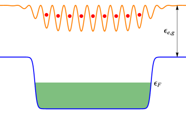
Figure 1: (Color online) Illustration of a magnetic impurity setup for ¹⁷³Yb atoms (schematic). Atoms in the ground-state ¹S₀ form a Fermi sea (Fermi energy $\epsilon_{F}$), while atoms in the excited-state ³P₀ are trapped in an optical potential and form a dilute concentration of localized magnetic impurities. $\epsilon_{\mathrm{e},\mathrm{g}}$ is the excitation energy (5) of the ³P₀ state.

The energy dispersion and density of states (DOS) for the (weakly confined) Yb(¹S₀) atoms read,

$$\epsilon_{k}~{}=~{}\frac{\hbar^{2}k^{2}}{2M},\ \ \rho(\epsilon)~{}=~{}\frac{Mk_{\epsilon}}{2\pi^{2}\hbar^{2}}.$$ (1)

Here $M$ is the atomic mass, $k=|\mathbf{k}|$, $\mathbf{k}=(k_{x},k_{y},k_{z})$, with $k_{\alpha=x,y,z}=\frac{\pi n_{\alpha}}{2L}$, in which $\{n_{\alpha}\}$ are integers and $k_{\epsilon}=\sqrt{2M\epsilon}/\hbar$.

As for the impurities, an Yb(³P₀) atom at position ${\bf R}=(X_{1},X_{2},X_{3})$ is trapped by an optical potential,

$$V_{\mathrm{e}}(\mathbf{R}) = -V_{\mathrm{e}}^{(0)}\sum_{\alpha}\sin^{2}\big{(}k_{\mathrm{e}}X_{\alpha}\big{)},$$ (2)

where $k_{\mathrm{e}}$ is the wave number of the laser light. The lowest energy level $\epsilon_{\mathrm{imp}}$ of the Yb(³P₀) atom is deep and close to the minimum of $V_{\mathrm{e}}(\mathbf{R})$, hence it can be approximated harmonic potential at lowest energy,

$$\epsilon_{\mathrm{imp}} = \frac{3}{2}~{}\hbar\Omega_{\mathrm{e}},$$ (3)

wherein the harmonic frequency and length are,

$$\hbar\Omega_{\mathrm{e}}~{}=~{}2\sqrt{{\mathcal{E}}_{\mathrm{e}}V_{\mathrm{e}}^{(0)}},\ \ \ \ \ k_{\mathrm{e}}a_{\mathrm{e}}~{}=~{}\bigg{(}\frac{{\mathcal{E}}_{\mathrm{e}}}{V_{\mathrm{e}}^{(0)}}\bigg{)}^{1/4},$$ (4)

with recoil energy ${\mathcal{E}}_{\mathrm{e}}=\frac{\hbar^{2}k_{\mathrm{e}}^{2}}{2M}.$  
Exchange interaction between the Yb(¹S₀) and Yb(³P₀) atoms is described in details in Ref. IK-TK-YA-GBJ-PRB-16 , but there, one of the parameters is chosen wrongly, leading to an incorrect conclusion. Here we correct it and explain how the exchange interaction can be optically controlled. Consider an Yb atom as a doubly ionized closed shell rigid ion and two valence electrons. The ground state ¹S₀ electron configuration is $6s^{2}$, whereas that of the excited state ³P₀ is $6s6p$. The excitation energy is

$$\epsilon_{\mathrm{e},\mathrm{g}} = \epsilon_{\mathrm{e}}-\epsilon_{\mathrm{g}}=2.14349~{}{\text{eV}}.$$ (5)

The positions of the ion core and the outer electrons are respectively specified by vectors $\mathbf{R}$, $\mathbf{r}_{\mathrm{a}}$ and $\mathbf{r}_{\mathrm{b}}$. In the adiabatic (Born-Oppenheimer) approximation (which is well substantiated in atomic physics), the wave function of a single Yb atom is expressed as a product of the wave functions of the rigid ion core (considered as a point particle of mass $M$), and that of the valence electrons. When one valence electron virtually tunnels from an Yb($6s^{2}$) atom to an Yb($6s6p$) atom we get an ionized Yb⁺($6s$) atom and a charged Yb^-($6s^{2}6p$) atom. The corresponding excitation energy is,

$$\Delta\varepsilon = \varepsilon_{\mathrm{ion}}-\varepsilon_{\mathrm{ea}}-\epsilon_{\mathrm{e},\mathrm{g}}~{}=~{}4.4107~{}{\mathrm{eV}},$$ (6)

where $\varepsilon_{\mathrm{ion}}=6.2542$ eV is the ionization energy of ytterbium Yb-spectrum-78 and $\varepsilon_{\mathrm{ea}}=-0.3$ eV is the electron affinity Electron-afinity-PhRep04 .

Such virtual tunneling of electrons between the atoms gives rise to anti-ferromagnetic exchange interaction between them. Following Ref. IK-TK-YA-GBJ-PRB-16 , we describe the exchange interaction by the potential

$$V_{\mathrm{exch}}^{\mathrm{(bare)}}(R)=g_{0}\zeta(R),$$ (7)

where

$$g_{0} = 2.821472~{}{\text{eV}}\times{\text{\AA}}^{3},$$

$$\zeta(R) = \frac{1}{Z}~{}\bigg{(}\frac{R}{r_{0}}\bigg{)}^{4\gamma}e^{-\kappa(R-r_{0})},$$

$$Z = \frac{4\pi r_{0}^{3}}{\big{(}\kappa r_{0}\big{)}^{4\gamma+3}}~{}\Gamma\big{(}4\gamma+3,\kappa r_{0}\big{)}~{}e^{\kappa r_{0}}.$$

Here $r_{0}$ is the classical turning point where the van der Waals potential vanishes [see Eq.  (8) below]. The parameters $\kappa$ and $\gamma$ are

$$\kappa=\kappa_{s}+\kappa_{p}=2.3199~{}{\text{\AA}}^{-1},$$

$$\gamma=\frac{1-\beta_{s}}{\beta_{s}}+\frac{1-\beta_{p}}{\beta_{p}}=1.2942,$$

where $\beta_{\mathrm{s}}=0.67799$, $\beta_{\mathrm{p}}=0.54966$, $\kappa_{\mathrm{s}}=1.2812$ Å^-1 and $\kappa_{\mathrm{p}}=1.0387$ Å^-1 IK-TK-YA-GBJ-PRB-16 .

Van der Waals interaction: The van der Waals interaction between the Yb atoms is modelled here by the Lennard-Jones potential vdW-Yb-PRA-08 ; vdW-Yb-PRA-14 ,

$$W^{\mathrm{(bare)}}(R) = \frac{C_{6}}{R^{6}}~{}\bigg{\{}\frac{\sigma^{6}}{R^{6}}-1\bigg{\}}-\frac{C_{8}}{R^{8}},$$ (8)

with $C_{6}=2.561\cdot 10^{3}E_{h}a_{B}^{6}$, $C_{8}=3.222465\cdot 10^{5}E_{h}a_{B}^{8}$ and $\sigma=9.0109361a_{B}$, where $E_{h}=27.211$ eV is the Hartree energy and $a_{B}=0.52918$ Å is the Bohr radius.

Light-assisted interaction: Controlling the strength and sign of the exchange interaction is achieved by subjecting the mixture of Yb atoms to a laser beam of frequency $\omega_{0}$ that is tuned to be close to the resonant frequency $\omega_{\mathrm{res}}=\Delta\varepsilon/\hbar$. Recall that $\Delta\varepsilon$ is the energy difference (6) between the two neutral atoms and the two ions. Concretely, $\frac{\omega_{\mathrm{res}}}{2\pi c}~{}=~{}35574.7~{}{\text{cm}}^{-1}.$

The interaction between the electromagnetic field (derived from a vector potential ${\bf A}$) and electrons in an atom is of the form Landau-Lifshitz-2 ,

$$H_{\mathrm{em}} = -\frac{e}{c}~{}\frac{\mathbf{p}\cdot\mathbf{A}}{m_{e}},$$

where $\mathbf{p}=-i\hbar\nabla$ is the electronic momentum operator and $m_{e}$ is the electronic mass. This interaction gives rise to tunneling of electrons between the atoms. When detuning $\Delta\omega=\omega_{0}-\omega_{\mathrm{res}}$ of the light frequency is much larger than the natural linewidth of the absorption line $\omega_{\mathrm{res}}$, tunnelling of electrons between the atoms is forbidden by the energy conservation law. In second order perturbation theory, the laser light induces an additional potential $W^{\mathrm{(ind)}}(R)$ and exchange interactions $V_{\mathrm{exch}}^{\mathrm{(ind)}}(R)$ between the neutral atoms,

$$W^{\mathrm{(ind)}}(R) = \frac{1}{\hbar\Delta\omega}~{}\Big{\{}t_{s,{\mathrm{ind}}}^{2}(R)+t_{p,{\mathrm{ind}}}^{2}(R)\Big{\}},$$ (9)

$$V_{\mathrm{exch}}^{\mathrm{(ind)}}(R) = \frac{2}{\hbar\Delta\omega}~{}t_{s,{\mathrm{ind}}}(R)~{}t_{p,{\mathrm{ind}}}(R).$$ (10)

The tunneling rates $t_{\mu,{\mathrm{ind}}}(R)$ ($\mu=s,p$) are,

$$t_{\mu,{\mathrm{ind}}}(R) = \frac{ev_{0}E_{0}}{4\pi\omega_{0}}~{}{\mathfrak{F}}_{\mu}(R),$$

where $v_{0}$=$\frac{\hbar}{m_{e}a_{B}}$=$0.00729735c$, $E_{0}$ is the amplitude of the laser’s electric field and the dimensionless functions ${\mathcal{F}}_{\mu}(R)$ are

$${\mathfrak{F}}_{\mu}(R)=a_{B}\int d^{3}\mathbf{r}~{}\psi_{\mu}^{*}\big{(}\big{|}\mathbf{r}-\mathbf{R}\big{|}\big{)}~{}\frac{\partial\psi_{\mu}(r)}{\partial z}.$$ (11)

The axis $z$ is chosen parallel to the vector $\mathbf{R}=\mathbf{R}_{\mathrm{g}}-\mathbf{R}_{\mathrm{e}}$. For the single-electron wave function $\psi_{\mu}(r)$, we use the asymptotic expression IK-TK-YA-GBJ-PRB-16 ,

$$\psi_{\mu}(r) = \sqrt{\frac{2{\mathcal{A}}~{}\kappa_{\mu}^{3}}{\pi~{}\Gamma\big{(}\frac{\beta_{\mu}+2}{\beta_{\mu}}\big{)}}}~{}\big{(}2\kappa_{\mu}r\Big{)}^{\frac{1-\beta_{\mu}}{\beta_{\mu}}}e^{-\kappa_{\mu}r},$$ (12)

where $\mu=s,p$ for the $6s$ and $6p$ electron, ${\mathcal{A}}=1.355$,

$$\beta_{\mathrm{s}}~{}=~{}0.67799,\ \ \ \ \ \kappa_{\mathrm{s}}~{}=~{}1.2812~{}{\text{\AA}}^{-1},$$

$$\beta_{\mathrm{p}}~{}=~{}0.54966,\ \ \ \ \ \kappa_{\mathrm{p}}~{}=~{}1.0387~{}{\text{\AA}}^{-1}.$$

It is useful to rewrite the (laser induced) potential and exchange contributions [$W^{\mathrm{(ind)}}(R)$ and $V_{\mathrm{exch}}^{\mathrm{(ind)}}(R)$] in the compact form,

$$W^{\mathrm{(ind)}}(R) = \frac{V_{0}}{2}~{}\Big{\{}{\mathcal{F}}_{s}^{2}(R)+{\mathcal{F}}_{p}^{2}(R)\Big{\}},$$ (13)

$$V_{\mathrm{exch}}^{\mathrm{(ind)}}(R) = V_{0}~{}{\mathcal{F}}_{s}(R)~{}{\mathcal{F}}_{p}(R),$$ (14)

where the coupling $V_{0}$ is given by,

$$V_{0}~{}=~{}\frac{2}{\hbar\Delta\omega}~{}\bigg{(}\frac{eE_{0}v_{0}}{4\pi\omega_{0}}\bigg{)}^{2}.$$ (15)

Hereafter we consider the case of blue detuning with $\Delta\omega>0$.

Scattering lengths: The van der Waals and exchange interactions yield “singlet” and “triplet” scattering lengths Scatt-Length-WKB-PRA93 ; vdW-Yb-PRA-08 ; IK-TK-YA-GBJ-PRB-16 ,

$$a_{\nu} = \bar{a}~{}\bigg{\{}1-\tan\Big{(}\Phi_{\nu}-\frac{\pi}{8}\Big{)}\bigg{\}},$$ (16)

where $\nu=S,T$ for the quantum states with antisymmetric (“singlet”) and symmetric (“triplet”) two-particle spin wave functions, and

$$\bar{a} = \frac{1}{2^{3/2}}~{}\frac{\Gamma\big{(}\frac{3}{4}\big{)}}{\Gamma\big{(}\frac{5}{4}\big{)}}~{}\bigg{(}\frac{MC_{6}}{\hbar^{2}}\bigg{)}^{1/4}~{}=~{}39.73~{}{\text{\AA}}.$$ (17)

The parameters $\Phi_{\nu}$ are,

$$\Phi_{\nu} = \int\limits_{R_{\nu}}^{\infty}K_{\nu}(R)~{}dR,$$ (18)

where

$$K_{\nu}(R) = \frac{1}{\hbar}~{}\sqrt{-M\big{[}W(R)+\eta_{\nu}V_{\mathrm{exch}}(R)\big{]}}.$$ (19)

In the above equation $W(R)=W^{\mathrm{(bare)}}(R)+W^{\mathrm{(ind)}}(R)$, $V_{\mathrm{exch}}(R)=V_{\mathrm{exch}}^{\mathrm{(bare)}}(R)+V_{\mathrm{exch}}^{\mathrm{(ind)}}(R)$, $\eta_{S}=1$ and $\eta_{T}=-1$. $R_{\nu}$ is the solution of equation $W(R_{\nu})+\eta_{\nu}V_{\mathrm{exch}}(R_{\nu})=0$.

When the intensity of the laser beam with frequency $\omega_{0}$ vanishes [i.e., when $V_{0}\to 0$], the scattering lengths are IK-TK-YA-GBJ-PRB-16

$$a_{S}~{}=~{}1878~{}a_{B},\ \ \ \ \ a_{T}~{}=~{}219.7~{}a_{B},$$ (20)

(where $a_{B}$ is the Boh’r radius) which agree well with the experimental results Scazza-Yb-3P0 ; Scazza-Yb-3P0-2015 .

Evaluating the scattering lengths for nonzero $V_{0}$, requires calculation of $V_{\mathrm{exch}}^{\mathrm{(ind)}}(R)$ and $W^{\mathrm{ind}}(R)$, eqs. (14) and (13). Substituting them into eq. (18) yields the quantity $\Phi_{\nu=S,T}$ as functions of $V_{0}$. This is carried out numerically, after which eq. (16) is employed to find the scattering lengths.

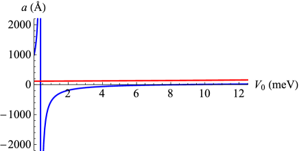
Figure 2: (Color online) Scattering lengths $a_{S}$ [blue curve] and $a_{T}$ [red curve] as functions of $V_{0}$.

The scattering lengths (16) calculated numerically are displayed in Fig. 2 as functions of $V_{0}$. It is seen that in the interval $V_{0}<12.5$ meV, there is a value of $V_{0}$ where $a_{S}$ is singular: $V_{{\mathrm{c}}}=0.3809$ meV. On the other hand, $a_{T}$ varies slowly within the interval $V_{0}<12.5$ meV.

Kondo Hamiltonian: Once the “singlet” and “triplet” scattering lengths are known, it is possible to construct the effective Kondo Hamiltonian, with explicit expressions for potential and exchange coupling constants denoted below as $g_{\mathrm{pot}}$ and $g_{\mathrm{exch}}$ respectively. Let us consider a degenerate Fermi gas of Yb(¹S₀) atoms, and one Yb(³P₀) atom localized at $\mathbf{R}_{\mathrm{e}}=0$ which plays a role of a magnetic impurity. Then the Kondo Hamiltonian is,

$$H_{K} = g_{\mathrm{pot}}\sum_{\mathbf{k},\mathbf{k}^{\prime}}\sum_{m}c_{\mathbf{k}^{\prime},m}^{{\dagger}}c_{\mathbf{k},m}+$$ (21)

$$+ g_{\mathrm{exch}}\sum_{\mathbf{k},\mathbf{k}^{\prime}}\sum_{m\neq m^{\prime}}X^{m,m^{\prime}}c_{\mathbf{k}^{\prime},m^{\prime}}^{{\dagger}}c_{\mathbf{k},m}+$$

$$+ g_{\mathrm{exch}}\sum_{\mathbf{k},\mathbf{k}^{\prime}}\sum_{m}Z^{m,m}c_{\mathbf{k}^{\prime},m}^{{\dagger}}c_{\mathbf{k},m}.$$

Here $c_{\mathbf{k},m}$ and $c_{\mathbf{k},m}^{{\dagger}}$ are annihilation and creation operators of itinerant atom with wave vector $\mathbf{k}$ and magnetic quantum number $m$. $X^{m,m^{\prime}}=|{m}\rangle\langle{m^{\prime}}|$ are Hubbard operators of the localized impurity, the ket $|m\rangle$ describes the impurity with magnetic quantum number $m$. $Z^{m,m}=X^{m,m}-\frac{1}{6}$. $g_{\mathrm{pot}}$ and $g_{\mathrm{exch}}$ are effective couplings of the potential and exchange interactions. Here $g_{\mathrm{exch}}>0$ denotes antiferromagnetic exchange interaction. The laser induced scattering lengths due to the short range interaction (21) are,

$$a_{\nu=S,T} = \frac{M}{4\pi\hbar^{2}}~{}\big{\{}g_{\mathrm{pot}}+\alpha_{\nu}~{}g_{\mathrm{exch}}\big{\}},$$ (22)

where $\alpha_{S}=-\frac{7}{6}$ and $\alpha_{T}=\frac{5}{6}$. Then the couplings $g_{\mathrm{pot}}$ and $g_{\mathrm{exch}}$ of the potential and exchange interactions are expressed is terms of the scattering lengths as,

$$g_{\mathrm{pot}}~{}=~{}\frac{\pi\hbar^{2}}{3M}~{}\Big{\{}5a_{S}+7a_{T}\Big{\}},$$ (23)

$$g_{\mathrm{exch}}~{}=~{}\frac{2\pi\hbar^{2}}{M}~{}\Big{\{}a_{T}-a_{S}\Big{\}}.$$ (24)

Eq. (24) shows that when $a_{T}>a_{S}$, the exchange interaction is anti-ferromagnetic and the Hamiltonian (21) gives rise to Kondo effect. When $a_{T}<a_{S}$, the exchange interaction is ferromagnetic and there is no Kondo effect.

Kondo temperature: When the exchange interaction (21) is anti-ferromagnetic (corresponding to regions in Fig. 2 where $a_{T}>a_{S}$), the Kondo temperature is Hewson-book ,

$$T_{K} = D_{0}~{}\exp\bigg{(}-\frac{1}{6~{}g_{\mathrm{exch}}~{}\rho(\epsilon_{F})}\bigg{)}.$$ (25)

Hereafter we assume that $2\hbar\Omega_{\mathrm{e}}<\epsilon_{F}$ [where $\epsilon_{F}$ is the Fermi energy and the harmonic frequency $\Omega_{\mathrm{e}}$ is given by eq. (4)], and therefore $D_{0}=2\hbar\Omega_{\mathrm{e}}/k_{B}$ plays a role of ultraviolet cutoff of the Kondo theory. The constant $\rho(\epsilon_{F})$ is the DOS (1) at the Fermi energy. A simple expression relating $T_{K}$ to the scattering lengths (valid for $a_{T}>a_{S}$) then reads,

$$T_{K} = D_{0}~{}\exp\Bigg{(}-\frac{\pi}{6k_{F}\big{(}a_{T}-a_{S}\big{)}}\Bigg{)},$$ (26)

where $a_{T}$ and $a_{S}$ as functions of $V_{0}$ are shown in Fig. 2.

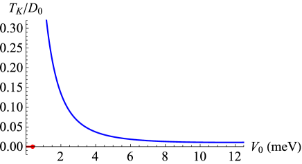
Figure 3: (Color online) Kondo temperature (blue curves) (26) as a function of $V_{0}$ for $\epsilon_{F}/k_{B}=100$ nK. The red segment indicates the interval $V_{0}<V_{\mathrm{c}}$ for which the Kondo effect is absent. Thus, the red dot denotes the critical potential $V_{{\mathrm{c}}}$ which separates the interval where Kondo effect is present from that where it is absent.

The Kondo temperature (26) calculated numerically is shown in Fig. 3, (blue curves). It is seen that the Kondo temperature sharply increases with decreasing $a_{S}$ [see Fig. 2]. In the red segment of $V_{0}$ where $a_{S}>a_{T}$ the Kondo effect is absent.

Conclusions: Tuning interaction strength in quantum impurity problems in cold atom systems cannot rely on the application of an external magnetic field (for driving Feshbach resonance), because it is detrimental for the Kondo effect. Hence, employing optical toolbox for controlling interaction strength in cold atom systems is a proper substitute. But so far it has been applied in numerous works mainly for studying bosonic systems. The quest for studying quantum (magnetic) impurity problems and Kondo physics requires a novel kind of controlling the exchange interaction. More concretely, it involves a subtle tuning of “singlet” and “triplet” scattering lengths, and identifying the conditions wherein $a_{S}<a_{T}$, for which the exchange interaction is antiferromagnetic.

This objective has been achieved here for an experimentally representative system. The feasibility to construct optically tuneable exchange interaction between itinerant ¹⁷³Yb(¹S₀) atoms and a localized ¹⁷³Yb(³P₀) impurity has been analyzed. “Singlet” and “triplet” scattering lengths as a function of $V_{0}$ (which is proportional to the light intensity) are explicitly calculated and the regions where $a_{S}<a_{T}$ in which the exchange interaction is antiferromagnetic are identified. With increasing intensity of light (from zero), the exchange interaction changes both in magnitude and in sign. The Kondo Hamiltonian is then constructed and the Kondo temperature is calculated in the intervals of $V_{0}$ where the exchange interaction is anti-ferromagnetic. It is shown that $T_{K}$ increases sharply before reaching an optical Feshbach resonance where the singlet scattering length approaches $-\infty$ .  
Acknowledgement We thank the authors of Refs.CIR1 ; CIR2 ; CIR3 ; CIR4 for drawing our attention to the CIR method. Prof. Y. Band is to be acknowledged for pointing out the relevance of spontaneous emission. This research is supported in part by an Israel Science Foundation grant 400/12.

.1 About spontaneous emission

Spontaneous emission is dangerous since it heats the atomic gas. In order to avoid this, we need to organize the procedure as follows:

(1) The frequency of detuning from the resonant frequency is needed to be large enough so that the decay rate due to spontaneous emission of a photon is very low.

(2) The ¹S₀ and ³P₀ quantum states have different electronic principal quantum numbers and spin states. Electric dipole transition between the singlet states ¹S₀ and ³P₀ is forbidden. Magnetic dipole transition can change the spin, but not the principal quantum number. Therefore, spontaneous quantum transition from ³P₀ to ¹S₀ state of Yb is virtually forbidden (or at least, the lifetime of the ³P₀ state is very long).

Note that the same problem exists also for a ”bare” mixture of Yb(¹S₀) and Yb(³P₀) atoms (without an additional laser light). However, applying an additional laser radiation makes the exchange interaction stronger and (possible) the lifetime shorter. So far, we do not know how to calculate the lifetime.

In an experimental work arXiv:1708.03810 CIR3 the authors write: “For the scattering of the ionization beam, we will try to estimate the scattering rates and compare it with our trap depths. Probably, we will have to choose a significant detuning as not to heat the atoms out of the trapping confinement.”

References

- (1) S. E. Pollack, D. Dries, M. Junker, Y. P. Chen, T. A. Corcovilos, and R. G. Hulet, Phys. Rev. Lett. 102, 090402 (2009).
- (2) Dan M. Stamper-Kurn and Masahito Ueda, Rev. Mod. Phys. 85, 1191 (2013).
- (3) J. Stenger, S. Inouye, D. M. Stamper-Kurn, H.-J. Miesner, A. P. Chikkatur and W. Ketterle, Nature 396, 345 (1998).
- (4) Simon Murmann, Andrea Bergschneider, Vincent M. Klinkhamer, Gerhard Zürn, Thomas Lompe, and Selim Jochim, Phys. Rev. Lett. 114, 080402 (2015).
- (5) Cheng Chin, Rudolf Grimm, Paul Julienne, and Eite Tiesinga, Rev. Mod. Phys. 82, 1225 (2010).
- (6) P. O. Fedichev, Yu. Kagan, G. V. Shlyapnikov, and J. T. M. Walraven, Influence of nearly resonant light on the scattering length in low-temperature atomic gases, Phys. Rev. Lett. 77, 2913 (1996).
- (7) L.-M. Duan, E. Demler, M. D. Lukin, Phys. Rev. Lett. 91, 090402 (2003); arXiv:cond-mat/0210564.
- (8) R. Ciuryło, E. Tiesinga, and P. S. Julienne, Phys. Rev. A 71, 030701(R) (2005).
- (9) Pascal Naidon and Françoise Masnou-Seeuws, Phys. Rev. A 73, 043611 (2006).
- (10) Thorsten Köhler, Krzysztof Góral, and Paul S. Julienne, Rev. Mod. Phys. 78, 1311 (2006).
- (11) M. Theis, G. Thalhammer, K. Winkler, M. Hellwig, G. Ruff, R. Grimm, J. Hecker Denschlag, Tuning the scattering length with an optically induced Feshbach resonance, Phys. Rev. Lett. 93, 123001 (2004); arXiv:cond-mat/0404514.
- (12) John L. Bohn and P. S. Julienne, Prospects for influencing scattering lengths with far-off-resonant light, Phys. Rev. A 56, 1486 (1997).
- (13) Felix H.J. Hall, Mireille Aymar, Nadia Bouloufa-Maafa, Olivier Dulieu, Stefan Willitsch, Light-assisted ion-neutral reactive processes in the cold regime: radiative molecule formation vs. charge exchange, Phys. Rev. Lett. 107, 243202 (2011); arXiv:1108.3739.
- (14) Adam Micah Kaufman, Radiofrequency dressing of atomic Feshbach resonances, Submitted to the Department of Physics of Amherst College in partial fulfilment of the requirements for the degree of Bachelors of Arts, 2009.
- (15) S. Blatt, T. L. Nicholson, B. J. Bloom, J. R. Williams, J. W. Thomsen, P. S. Julienne, and J. Ye, Phys. Rev. Lett. 107, 073202 (2011).
- (16) S. Trotzky, P. Cheinet, S. Fölling, M. Feld, U. Schnorrberger, A. M. Rey, A. Polkovnikov, E. A. Demler, M. D. Lukin, I. Bloch, Science 319, 295 (2008).
- (17) A. C. Hewson, The Kondo Problem to Heavy Fermions (Cambridge University Press, Cambridge, 1993).
- (18) J. Bauer, C. Salomon and E. Demler, Phys. Rev. Lett. 111, 215304 (2013).
- (19) I. Kuzmenko, T. Kuzmenko, Y. Avishai and K. A. Kikoin, Phys. Rev. B 91, 165131 (2015); arXiv:1402.0187.
- (20) Igor Kuzmenko, Tetyana Kuzmenko, Yshai Avishai and Gyu-Boong Jo, Phys. Rev. B 93, 115143 (2016); arXiv:1512.00978.
- (21) Igor Kuzmenko, Tetyana Kuzmenko, Yshai Avishai and Gyu-Boong Jo, Phys. Rev. B 97, 075124 (2018).
- (22) Ren Zhang, Deping Zhang, Yanting Cheng, Wei Chen, Peng Zhang, and Hui Zhai, Phys. Rev. A 93, 043601 (2016); arXiv:1509.01350.
- (23) Yanting Cheng, Ren Zhang, Peng Zhang, and Hui Zhai, Phys. Rev. A 96, 063605 (2017); arXiv:1705.06878.
- (24) Luis Riegger, Nelson Darkwah Oppong, Moritz Hfer, Diogo Rio Fernandes, Immanuel Bloch and Simon Flling, arXiv:1708.03810.
- (25) Qing Ji, Ren Zhang, Xiang Zhang, Wei Zhang, arXiv:1809.00471.
- (26) W. F. Meggers and J. L. Tech, J. Res. Natl. Bur. Stand. (U.S.) 83, 13 (1978).
- (27) T. Andersen, “Atomic negative ions: Structure, dynamics and collisions”. Physics Reports 394, 157 (2004).
- (28) Masaaki Kitagawa, Katsunari Enomoto, Kentaro Kasa, Yoshiro Takahashi, Roman Ciuryło, Pascal Naidon, and Paul S. Julienne, Phys. Rev. A 77, 012719 (2008); arXiv:0708.0752.
- (29) G. F. Gribakin and V. V. Flambaum, Phys. Rev. A 48, 546 (1993).
- (30) F. Scazza, C. Hofrichter, M. Fofer, P. C. De Groot, I. Bloch, and S. Folling, Nature Physics 10, 779 (2014); ibid: correction notice, (2015).
- (31) M. Höfer, L. Riegger, F. Scazza, C. Hofrichter, D. R. Fernandes, M. M. Parish, J. Levinsen, I. Bloch, and S. Fölling, Phys. Rev. Lett. 115, 265302 (2015).
- (32) S. G. Porsev, M. S. Safronova, A. Derevianko, and C. W. Clark, Phys. Rev. A 89, 012711 (2014).
- (33) L. D. Landau and E. M. Lifshitz, The Classical Theory of Fields, Course of Theoretical Physics, Volume 2. (Pergamon Press, 1971). pp. 44-46.