Environmental design principles for efficient excitation energy transfer in dimer and trimer pigment-protein molecular aggregates and the relation to non-Markovianity

Abstract

Lately there has been an interest in studying the effects and mechanisms of environment-assisted quantum transport, especially in the context of excitation energy transfer (EET) in pigment-protein molecular aggregates. Since these systems can be seen as open quantum systems where the dynamics is within the non-Markovian regime, the effect of non-Markovianity on efficient EET as well as its role in preserving quantum coherence and correlations has also been investigated in recent works. In this study, we explore optimal environments for efficient EET between end sites in a number of dimer and trimer model pigment-protein molecular aggregates when the EET dynamics is modeled by the HEOM-method. For these optimal environmental parameters, we further quantify the non-Markovianity by the BLP-measure to elucidate its possible connection to efficient EET. We also quantify coherence in the pigment systems by means of the measure $l_{1}-$norm of coherence to analyze its interplay with environmental effects when EET efficiency is maximal. Our aim is to investigate possible environmental design principles for achieving efficient EET in model pigment-protein molecular aggregates and to determine whether non-Markovianity is a possible underlying resource in such systems. We find that the structure of the system Hamiltonian (i.e., the pigment Hamiltonian parameter space) and especially, the relationship between the site excitation energies, determines whether one of two specific environmental regimes is the most beneficial in promoting efficient EET in these model systems. In the first regime, optimal environmental conditions are such that the EET dynamics in the system is left as coherent as possible. In the second regime, the most advantageous role of the environment is to drive the system towards equilibrium as fast as possible. In reality, optimal environmental conditions may involve a combination of these two effects. We cannot establish a relation between efficient EET and non-Markovianity, i.e., non-Markovianity cannot be regarded as a resource in the systems investigated in this study.

PACS numbers: 03.65.Yz, 05.60.Gg

I Introduction

The time evolution of a quantum system interacting with an environment is of interest in many research fields studying open quantum systems, such as quantum information theory and condensed matter physics (Breuer and Petruccione, 2002). Generally, the interaction with a macroscopic environment, i.e., an environment consisting of infinitely many degrees of freedom, has mainly been seen as a source of dissipation and decoherence in the system, leading to destruction of desirable quantum resources such as quantum entanglement. The main focus of technological developments of quantum systems for applications such as quantum computation has consequently been to isolate the system from its environment.

Recently, it has been recognized that in some quantum systems, environmental effects may help to protect, or even create, quantum resources in form of quantum correlations and coherence in the system. Well known examples of such systems are certain photosynthetic complexes, each consisting of a network of pigments (light absorbing organic molecules) held together by a protein scaffold, forming a molecular aggregate. Despite the fact that the network of pigments is strongly coupled to a macroscopic environment at physiological temperature, long-lasting quantum coherence - which may act as a resource in these complexes - has been experimentally verified (Engel et al., 2007; Hayes et al., 2010; Panitchayangkoon et al., 2010, 2011).

In a photosynthetic complex, one of the pigments absorbs a photon which is transferred as excitation energy through the network of pigments until it reaches a pigment that is functioning as an end site. In connection to this pigment in the network, the excitation is captured by a reaction center and converted to chemical energy. The overall efficiency of photosynthetic complexes hence depends, among other things, on how efficient an excitation can be transferred from the initially excited pigment to the pigment in contact with the reaction center. Photosynthetic complexes are known to convert excitation energy to chemical energy with high efficiency (Chain and Arnon, 1977) which has created an interest in studying their properties and trying to mimic their features in artificial photosynthesis-technology. It is believed that quantum coherence together with environmental effects enables such an efficient excitation energy transfer (EET) among the pigments in the network and many studies have tried to reveal how quantum coherence, different environmental interactions and EET efficiency are related to each other (Qin et al., 2014; Plenio and Huelga, 2008; Caruso et al., 2009; Chin et al., 2010; Sinayskiy et al., 2012; Marais et al., 2013; Wu et al., 2010; Rebentrost et al., 2009a, b; Mohseni et al., 2008; Dijkstra and Tanimura, 2012; Shabani et al., 2012; Mohseni et al., 2014).

The standard computational treatment to study the effects of an environment on an open quantum system, which has been used in the study of pigment-protein molecular aggregates in Refs. (Rebentrost et al., 2009b; Plenio and Huelga, 2008; Caruso et al., 2009; Wu et al., 2010; Rebentrost et al., 2009a; Mohseni et al., 2008), has been to employ Markovian master equations to model the dynamics. The Markovian approximation is to assume that the environment is in equilibrium during the time evolution of the system. For some processes, such as EET in photosynthetic complexes where the strength of the system-environment interaction is of the same order as the intra-system interactions, Markovian master equations are not sufficient to capture relevant environmental effects. In order to accurately take those effects into account, the dynamics has to be modeled by master equations within the non-Markovian regime. As a result, there is a possibility for information to flow back-and-forth between the system and the environment during the time evolution of the system. Hence, environmental-induced revivals of quantities such as coherence and correlations within the system may occur.

In the case of photosynthetic complexes, the need for non-Markovian master equations to capture the behavior of the system-environment interactions in a realistic manner has resulted in developments of new theoretical methods. Especially the hierarchical equations of motion (HEOM) method, originally derived in Refs. (Tanimura and Kubo, 1989a, b; Tanimura, 1990) and then extended in Refs. (Ishizaki and Fleming, 2009a, b), has served as the benchmarking method to model EET in photosynthetic complexes.

Non-Markovian dynamics has been found to be a resource in some processes. Examples include entanglement generation (Paz and Roncaglia, 2008; Valido et al., 2013a, b; Bellomo et al., 2007; Huelga et al., 2012), information transfer in a noisy channel (Maniscalco et al., 2007; Bylicka et al., 2014; Caruso et al., 2014) and quantum communication (Laine et al., 2014; Liu et al., 2013). In Ref. (Thorwart et al., 2009) it is shown that non-Markovianity can function as a resource for prolonging the duration of coherence in a dimer pigment-protein model system. Non-Markovian effects in pigment-protein molecular aggregates have also been studied in Refs. (Chen et al., 2014; Rebentrost and Aspuru-Guzik, 2011; Mujica-Martinez et al., 2013).

As in the case of any potential quantum resource, it is crucial to be able to quantify non-Markovian effects in a system in order to be able to distinguish different environments in terms of their ability to function as a resource. Indeed, a number of different measures of non-Markovianity has been developed and proposed (Breuer et al., 2009; Rivas et al., 2010; Rajogopal et al., 2010). One that has been frequently used in studies of non-Markovianity is the BLP-measure (Breuer et al., 2009). It is based on the observation that the distinguishability of two initial states can never increase under a Markovian evolution. The distinguishability is quantified by the trace distance and an increase in the trace distance in a certain time interval is interpreted as a backflow of information from the environment to the system.

In this study, we investigate numerically how the parameters describing the environment and its coupling to the system influence EET efficiency between end sites in a network of $N$ ($N=2,3$) pigments in a protein scaffold when the HEOM method is used to model the EET dynamics. Within a range of possible environmental parameters, we seek for an optimum in the efficiency of the EET. We investigate a number of pigment configurations (defined by the pigments excitation energies and inter-pigment couplings) in order to evaluate how optimal environmental parameters may differ depending on the system under consideration. We further determine whether the dynamics imposed by the optimal environmental parameters (with respect to EET efficiency) is within the non-Markovian regime or not. To explore the interplay between coherence and environmental effects, as well as the possible connection between coherence and non-Markovianity, we quantify the amount of coherence in our systems by the $l_{1}$-norm of coherence (Baumgratz et al., 2014).

This study attempts to reveal design principles on how to create environmental conditions for efficient EET in pigment-protein molecular aggregates. Further, we aim to evaluate the possible role of non-Markovianity for efficient EET in such aggregates. The results can hopefully be useful for gaining insights on how to design artificial molecular aggregates for light harvesting.

II Systems

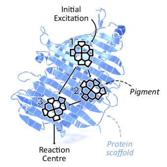
Figure 1: Schematic illustration of EET in a trimer pigment-protein molecular aggregate.

The systems considered in this study are networks of ${\color[rgb]{1,0,0}{\color[rgb]{0,0,0}N}}$ ($N=2,3$) sites where each site represents a pigment. These two types of systems can capture both pure quantum tunneling between pigments (dimer, i.e., $N=2$) and interference between different pathways (trimer, i.e., $N=3$), which are two important mechanisms in EET. A general trimer system ($N=3$) is illustrated in Fig. 1 along with the EET direction and possible EET pathways. The illustration also shows how the pigments are attached to a protein scaffold, which acts as the environment.

Each pigment is modeled as a two-level-system consisting of a ground state, $\ket{\Psi_{g}}$, and an excited state, $\ket{\Psi_{e}}$. The Hamiltonian of the full $N$-site system is assumed to be given by (Renger et al., 2001)

$$\hat{H}_{S}=\underset{i}{\sum}E_{i}\ket{i}\bra{i}+\underset{i\neq j}{\sum}J_{ij}\ket{i}\bra{j},$$ (1)

where $E_{i}$ is the excitation energy of site $i$, i.e., the energy required to excite site $i$ from $\ket{\Psi_{g}}$ to $\ket{\Psi_{e}}$, and $J_{ij}$ is the coupling (in reality, the electrostatic dipole-dipole coupling) of the two sites. The state $\ket{i}$ is equivalent to the state $\ket{\Psi_{g}^{1}\ldots\Psi_{e}^{i}\ldots\Psi_{g}^{N}}$, i.e., pigment $i$ is in its excited state while the rest of the pigments in the aggregate are in their ground states.

A well known natural pigment-protein molecular aggregate is one of the monomers in the Fenna-Matthews-Olson (FMO) complex (Fenna et al., 1974). It is commonly used as a model system for photosynthetic EET (Caruso et al., 2010; Sarovar et al., 2010; Fassioli and Olaya-Castro, 2010; Baker and Habershon, 2015; Chen et al., 2013; Rebentrost et al., 2009b; Plenio and Huelga, 2008; Caruso et al., 2009; Chin et al., 2010; Marais et al., 2013; Wu et al., 2010; Rebentrost et al., 2009a; Mohseni et al., 2008; Dijkstra and Tanimura, 2012; Shabani et al., 2012; Mohseni et al., 2014; Shabani et al., 2014; Wu et al., 2012; Mujica-Martinez et al., 2013; Rebentrost and Aspuru-Guzik, 2011) and consists of seven pigments arranged in such a way that there are two different routes for an initial excitation to be transferred to the reaction centre. The first of these two routes consists of pigments $1$, $2$ and $3$, where the initial excitation is located on pigment $1$ and pigment $3$ is in contact with the reaction centre, and the second route involves pigment $4$, $5$, $6$ and $7$ (Wu et al., 2012). Because the second route has an energy downhill structure, while the first route has an energy barrier between the first two sites which might require quantum tunneling, we choose to look at a model system consisting of $N$ sites that captures the features of the first EET route in a FMO-complex monomer. For the dimer case, these are: $\left|E_{1}-E_{2}\right|\sim\left|J_{12}\right|$. We refer to this system Hamiltonian as $\hat{H}_{{\rm{FMO}}}^{(2)}$. In the trimer case, we further have $E_{1,2}>E_{3},$ $\left|J_{12}\right|>\left|J_{23}\right|>\left|J_{13}\right|$, with Hamiltonian referred to as $\hat{H}_{{\rm{FMO}}}^{(3)}.$

In a recent study (Bengtson and Sjöqvist, 2017), the optimal Hamiltonian parameter space for a dimer and trimer pigment aggregate with respect to EET efficiency and time-averaged coherence in a closed system were found. We also investigate these systems, whose Hamiltonians are referred to as $\hat{H}_{{\rm{E}}}^{(N)}$ and $\hat{H}_{{\rm{C}}}^{(N)}$, respectively, where $N=2,3$. The specific Hamiltonian parameters for all six systems investigated in this study can be found in Tab. 1 (dimers) and Tab. 2 (trimers).

Table 1: Hamiltonian parameters for dimer systems. All values are given in units of ${\rm{cm}}^{-1}$.

Hamiltonian	$\mathbf{E_{1}-E_{2}}$	$\mathbf{J_{12}}$
$\hat{H}_{{\rm{FMO}}}^{(2)}$	$-100$	$-100$
$\hat{H}_{{\rm{E}}}^{(2)}$	$0$	$100$
$\hat{H}_{{\rm{C}}}^{(2)}$	$144$	$100$

Table 2: Hamiltonian parameters for trimer systems. All values are given in units of ${\rm{cm}}^{-1}$.

Hamiltonian	$\mathbf{E_{1}-E_{3}}$	$\mathbf{E_{2}-E_{3}}$	$\mathbf{J_{12}}$	$\mathbf{J_{23}}$	$\mathbf{J_{13}}$
$\hat{H}_{{\rm{FMO}}}^{(3)}$	$200$	$300$	$-100$	$50$	$0$
$\hat{H}_{{\rm{E}}}^{(3)}$	$0$	$0$	$100$	$100$	$0$
$\hat{H}_{{\rm{C}}}^{(3)}$	$40$	$-160$	$-100$	$-20$	$-100$

III Modeling and optimizing the EET efficiency

Figure 2: Physical interpretation of the parameters in HEOM. Left: Excitation from the ground state, $\ket{\Psi_{g}}$, to the excited state, $\ket{\Psi_{e}}$, of a pigment. Since the transition occurs vertically, the excitation of the electronic state is accompanied by excitation of vibrational (phonon) states. Relaxation of the vibrationally excited states releases reorganization energy, $\lambda$, which is proportional to the displacement, $d$, of the equilibrium configuration. Right: The parameter $\tau$ governs the decay rate of vibrationally excited states. At $t=\tau$, there is a probability ($P_{{\rm{relax}}}$ in the figure) of $1-\nicefrac{{1}}{{e}}$ that all vibrationally excited states have relaxed to their vibrational ground states.

The EET in the systems is modeled using the HEOM-method (Ishizaki and Fleming, 2009a, b) where the parameters representing the environment and its coupling to the system are varied in order to optimize EET efficiency. In the derivation of the HEOM method, the protein environment is modeled as a set of harmonic oscillator modes, i.e., phonons. EET between sites in the network occurs via non-equilibrium phonon states in accordance with vertical Franck-Condon transitions. The phonons are locally and linearly coupled to each site and when they relax to their equilibrium states, reorganization energy, denoted by $\lambda$, is released to the environment. Excitation- and de-excitation processes, including the release of the reorganization energy, of a pigment are shown in Fig. 2. The reorganization energy characterizes the strength of the system-environment coupling; a low value of $\lambda$ corresponds to a coherent EET dynamics.

The phonon relaxation dynamics is characterized by the parameter $\tau=\gamma^{-1}$, which determines the time scale of the environmental fluctuations. The physical meaning of $\tau$ is shown in Fig. 2, where it can be seen that the smaller $\tau$ is, the faster will a major part of the phonons relax to equilibrium. The environment is further described by its temperature, $T$, which defines the thermal equilibrium of the environment. Even though each site has its own, local environment, the parameters describing the environment ($\lambda,$ $\tau$ and $T$) are taken to be the same for all sites. A summary of the environmental parameters used in HEOM are found in Tab. 3.

The density operator, $\hat{\rho}$, describing the EET dynamics in the network of pigments is found by solving a set of HEOM, where the number of coupled equations are determined by a truncation condition (Ishizaki and Fleming, 2009a, b). This condition neglects phonon states much higher in energy than the characteristic frequency of the pigment-system.

The ranges of the temperature and the reorganization energy are chosen to be

$$250\,{\rm{K}}\leq T\leq 300\,{\rm{K}}$$ (2)

and

$$20\,{\rm{cm}^{-1}}\leq\lambda\leq 220\,{\rm{cm}^{-1}}.$$ (3)

In this way we interpolate between system-environment coupling strengths corresponding to EET dynamics in the coherent regime (where $\lambda$ is significantly smaller than the strongest inter-site couplings) and those corresponding to the incoherent regime (where $\lambda$ is significantly larger than the strongest inter-site couplings). The temperature is chosen to be within natural conditions and below temperatures where the protein scaffold would denature and hence, the 3D-structure of the pigment-protein aggregate would be destroyed. The range of the parameter $\tau$ is chosen such that the high temperature condition is fulfilled, which is a requirement to use HEOM in the form presented here (Ishizaki and Fleming, 2009a, b), i.e.,

$$\tau>\hbar\beta,\>\beta=k_{B}T,$$ (4)

where $k_{B}$ is Boltzmann’s constant. At $T=250\,{\rm{K}}$ (which is the critical temperature according to Eq. 4 in this case), the above condition requires that $\tau>31\,{\rm{fs}}.$ To be within this regime with clear margin, we use

$$50\,{\rm{fs}}\leq\tau\leq 500\,{\rm{fs}}$$ (5)

in our calculations. Due to numerical limitations, the parameter step-sizes are $\Delta T=2.5\,{\rm{K}},\>\Delta\lambda=10\,{\rm{cm}^{-1}},\>\Delta\tau=25\,{\rm{fs}}$ in the dimer systems and $\Delta T=5\,{\rm{K}},\>\Delta\lambda=20\,{\rm{cm}^{-1}},\>\Delta\tau=50\,{\rm{fs}}$ in the trimer systems. Further, we consider EET on the time scale of $1\>{\rm{ps}}$, i.e., $0\>{\rm{fs}}\leq t\leq 1000\>{\rm{fs}},$ which is a time scale widely accepted for EET in photosynthetic complexes.

Excitation of site $1$ is taken as initial condition for the EET dynamics. The convergence of the numerical solution is tested at critical values of $\lambda,$ $\tau$ and $T$ prior to performing the calculations for the full parameter ranges.

We also compare the time evolution of the site-populations to the corresponding populations at equilibrium ($t\rightarrow\infty$), which is defined by the system Hamiltonian (without environment),

$$\hat{\rho}_{{\rm{eq}}}=\frac{e^{-\beta\hat{H}_{S}}}{Z},$$ (6)

$$Z={\rm{Tr}}(e^{-\beta\hat{H}_{S}}).$$ (7)

Table 3: Summary of environmental parameters used in HEOM.

Parameter description	Symbol	Unit
System-environment coupling	$\lambda$	${\rm{cm}^{-1}}$
Environmental timescale	$\tau$	${\rm{\rm{fs}}}$
Environmental temperature	$T$	${\rm{K}}$

IV Quantifying efficiency, non-Markovianity and coherence

In this section we describe how we quantify EET efficiency (section IV.1), non-Markovianity (section IV.2) and coherence (section IV.3).

IV.1 Quantifying efficiency

The efficiency for transferring the initial state, $\hat{\rho}_{i}=\ket{1}\bra{1}$, into the target state, $\hat{\rho}_{f}=\ket{N}\bra{N}$, is quantified by fidelity, $F$, (Nielsen and Chuang, 2010) which takes the form

$$F(\hat{\rho})={\rm{Tr}}\sqrt{\sqrt{\hat{\rho}_{f}}\hat{\rho}\sqrt{\hat{\rho}_{f}}},$$ (8)

where $\hat{\rho}$ is the resulting state when $\hat{\rho}_{i}$ is evolved in time for a certain set of parameters $T$, $\lambda$ and $\tau$. Since the target state, $\hat{\rho}_{f}$, is a pure state, the expression in Eq. 8 is reduced to

$$F(\hat{\rho})=\sqrt{\bra{N}\hat{\rho}\ket{N}}.$$ (9)

IV.2 Quantifying non-Markovianity

A commonly used quantifier of non-Markovianity, based on distinguishability, was introduced by Breuer, Laine and Piilo (Breuer et al., 2009) and is consequently referred to as the BLP-measure in literature. It is derived from the observation that for all completely positive and trace-preserving maps, $\Phi$, the following holds (Ruskai, 1994);

$$D(\Phi(\hat{\rho}_{1}),\Phi(\hat{\rho}_{2}))\leq D(\hat{\rho}_{1},\hat{\rho}_{2}),$$ (10)

where $D$ is the trace distance, defined as (Nielsen and Chuang, 2010)

$$D(\hat{\rho}_{1},\hat{\rho}_{2})=\frac{1}{2}{\rm{Tr}}\left|\hat{\rho}_{1}-\hat{\rho}_{2}\right|.$$ (11)

Hence, the trace distance - which monitors the distinguishability of two states - will be a monotonically decreasing function of time. Any deviation from this behavior might be interpreted as a backflow of information and hence, a non-Markovian time evolution. In (Breuer et al., 2009), the measure of non-Markovianity of a dynamical map, $\Phi$, is defined as

$$\mathit{\mathrm{\mathcal{N}}}(\Phi)=\underset{\hat{\rho}_{1}(0),\hat{\rho}_{2}(0)}{\max}\underset{\sigma>0}{\int}\sigma[t,\hat{\rho}_{1}(0),\hat{\rho}_{2}(0)]\,dt,$$ (12)

where $\hat{\rho}_{1}(0)$ and $\hat{\rho}_{2}(0)$ are two initial states and

$$\sigma[t,\hat{\rho}_{1}(0),\hat{\rho}_{2}(0)]=\frac{d}{dt}D(\hat{\rho}_{1},\hat{\rho}_{2}).$$ (13)

The integral in Eq. 12 is optimized over all possible pairs of initial states to form a measure that only captures the features of the dynamics. The physical and mathematical structure of optimal state pairs is studied in Ref. (Wißmann et al., 2012). It is shown that an optimal pair of initial states will be orthogonal (i.e., the states can be described by density operators with orthogonal support), which implies that such a state pair must belong to the boundary, $\partial\mathcal{M}$, of the state space $\mathcal{M}$ of the density operators describing states of the system. Optimal state-pairs will fulfill $D(\hat{\rho}_{1}(0),\hat{\rho}_{2}(0))=1$, i.e., they are initially completely distinguishable. In this study, we have used the results in (Wißmann et al., 2012) in the optimization procedure.

In practice, we compute $\mathcal{N}$ by maximizing the integral of $\sigma[t,\hat{\rho}_{1}(0),\hat{\rho}_{2}(0)]$ over a random sample of initial state pairs. The orthogonality condition mentioned above is taken into account by using that any pair of density matrices $(\rho_{a},\rho_{b})$ with orthogonal support can be written as

$$\left\{\begin{array}[]{l}\rho_{a}=U\tilde{\rho}_{a}U^{\dagger}\\ \rho_{b}=U\tilde{\rho}_{b}U^{\dagger}\end{array}\right.,$$ (14)

where $\tilde{\rho}_{a}$ and $\tilde{\rho}_{b}$ are density matrices of the forms

$$\tilde{\rho}_{a}=\mathrm{diag}(\lambda_{1},\ldots,\lambda_{m},0,\ldots,0)$$ (15)

and

$$\tilde{\rho}_{b}=\mathrm{diag}(0,\ldots,0,\lambda_{m+1},\ldots,\lambda_{N}),$$ (16)

and $U$ is an element of the special unitary group of degree $N$, SU($N$). Conversely, it also holds that any pair of matrices generated according to the above prescription are density matrices with orthogonal support. The set of all orthogonal state pairs of size $N$ can therefore be parameterized by parametrizing SU($N$). In the present work, for the $N=2$ case, we choose the parametrization

$$U=\left[\begin{array}[]{cc}\cos\theta e^{i\phi_{1}}&-\sin\theta e^{-i\phi_{2}}\\ \sin\theta e^{i\phi_{2}}&\cos\theta e^{-i\phi_{1}}\end{array}\right],$$ (17)

$$0\leq\theta\leq\pi/2,\leavevmode\nobreak\ 0\leq\phi_{1},\phi_{2}\leq 2\pi,$$ (18)

whereas for the $N=3$ case we choose the analogous parametrization (also in terms of angles $\theta_{i}$ and phases $\phi_{i}$) given in Ref. (Bronzan, 1988). The sample of initial state pairs used for evaluating $\mathcal{N}$ is then constructed by drawing $\lambda_{i}$, $\theta_{i}$ and $\phi_{i}$ from a uniform distribution. Due to the simplicity of the present approach (for example, we do not assure that the distribution of initial state pairs is uniform) combined with the rather small sample size ($10^{5}$ and $10^{4}$ pairs for $N=2$ and $N=3$, respectively), we shall regard the values we obtain for $\mathcal{N}$ only as estimates of the corresponding true values.

IV.3 Quantifying coherence

Following the work of Ref. (Baumgratz et al., 2014), the $l_{1}$-norm of coherence is used to quantify the amount of coherence in the system. For a system described by a density operator, $\hat{\rho}$, the $l_{1}$-norm of coherence is given by

$$C_{l_{1}}^{(\psi)}(\hat{\rho})=\underset{\underset{i\neq j}{i,j}}{\sum}\left|\bra{\psi_{i}}\hat{\rho}\ket{\psi_{j}}\right|=2\underset{i<j}{\sum}\left|\rho_{ij}\right|,$$ (19)

where $\ket{\psi_{i}}$ and $\ket{\psi_{j}}$ are two quantum states in the set of the chosen basis states $\left\{\ket{\psi_{i}}\right\}$.

Since EET occurs in the site basis, coherence in the site basis, $C_{l_{1}}^{(s)}$, is of interest. Especially, we study local coherence,

$$C_{l_{1},ij}^{(s)}(\hat{\rho})=2\left|\rho_{ij}\right|,$$ (20)

between sites $i$ and $j$, where $\ket{\psi_{i}}=\ket{i}$ and $\ket{\psi_{j}}=\ket{j}$. Mathematically, the local coherence between two sites equals entanglement as quantified by concurrence (Wootters, 1998), i.e., the amount of entanglement between sites can be detected by this measure.

Furthermore, coherence in the exciton basis (the eigenbasis of the system Hamiltonian), $C_{l_{1}}^{(e)}$, is investigated. In a closed system, coherence in the exciton basis will be constant in time since the excitons are stationary solution of the Schrödinger equation. Hence, any time dependence of coherence in the exciton basis will be due to environmental effects and may be seen as a in-and-out flow of information to the system.

V Results and discussion

In presenting our results, we use the following notations to describe our findings:

• $F_{{\rm{OS,max}}}$$\left(F_{{\rm{OS,min}}}\right)$ denotes the maximal (minimal) efficiency obtained for each dimer and trimer system when all environmental parameters ($\lambda$, $\tau$ and $T$) as well as the time ($t$) are optimized in the open system (OS). The corresponding optimal parameter values are reported in the same manner, where for example $T_{{\rm{OS,max}}}$ is the temperature for which $F_{{\rm{OS,max}}}$ is achieved. When the efficiency is optimized only over certain parameters, while the dependencies on the others are retained, we show the free parameters as a superscript in the already introduced notations. For example, the efficiency optimized over $T$ and $t$ is denoted $F_{{\rm{OS,max}}}^{(\lambda,\tau)}$while the efficiency optimized over $\lambda$, $\tau$ and $T$ is denoted $F_{{\rm{OS,max}}}^{(t)}$.

• For the maximal (minimal) efficiency in the closed system (CS) (only optimized over $t$) we use the notation $F_{{\rm{CS,max}}}$$\left(F_{{\rm{CS,min}}}\right)$. The efficiency reached in the long-time limit (at equilibrium population), as calculated by Eq. 6, is denoted $F_{{\rm{eq}}}$.

• Coherence, $C_{l_{1}}^{(\psi)}$, is always shown for the optimal values (with respect to efficiency) of $\lambda$, $\tau$ and $T$ and its time dependence will be shown explicitly.

• Non-Markovianity is reported for environmental parameter values corresponding to maximal and minimal efficiency, and is denoted $\mathcal{N}_{{\rm{OS,max}}}$ and $\mathcal{N}_{{\rm{OS,min}}},$ respectively. For parameter values corresponding to maximal efficiency, we report trace distance as $D_{{\rm{OS,max}}}$.

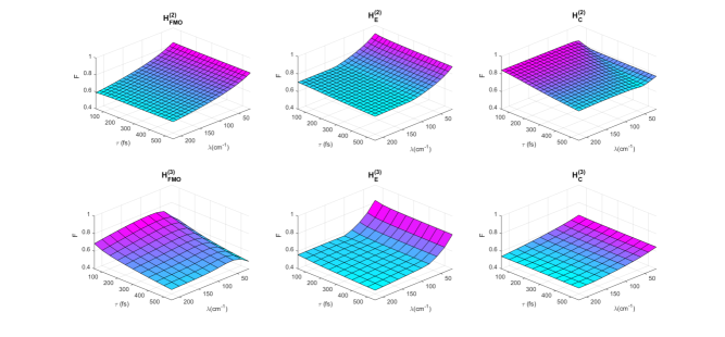
Figure 3: $F_{{\rm{OS,max}}}^{(\lambda,\tau)}$ as a function of $\lambda$ and $\tau$ for $\hat{H}_{{\rm{FMO}}}^{(N)}$, $\hat{H}_{{\rm{\rm{E}}}}^{(N)}$ and $\hat{H}_{{\rm{C}}}^{(N)}$. The upper panel shows results for the dimer systems and the lower panel shows results for the trimer systems.

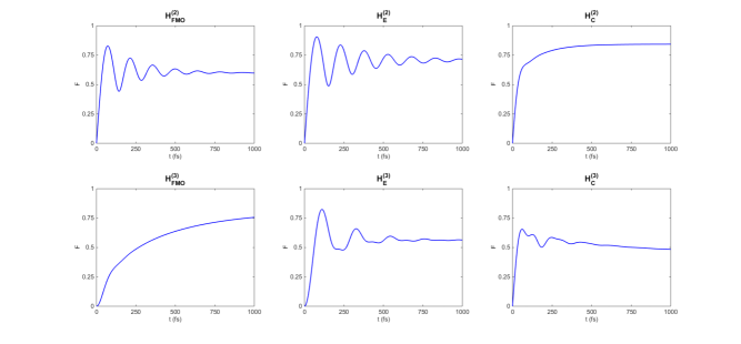
Figure 4: $F_{{\rm{OS,max}}}^{(t)}$ as a function of $t$ for $\hat{H}_{{\rm{FMO}}}^{(N)}$, $\hat{H}_{{\rm{E}}}^{(N)}$ and $\hat{H}_{{\rm{C}}}^{(N)}$. The upper panel shows results for the dimer systems and the lower panel shows results for the trimer systems.

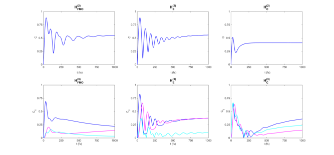
Figure 5: $C_{l_{1},ij}^{(s)}$ as a function of $t$ for $\hat{H}_{{\rm{FMO}}}^{(N)}$, $\hat{H}_{{\rm{\rm{E}}}}^{(N)}$ and $\hat{H}_{{\rm{C}}}^{(N)}$. The upper panel shows results for the dimer systems and the lower panel shows results for the trimer systems. Here, $C_{l_{1},12}^{(s)}$ (blue) $C_{l_{1},23}^{(s)}$ (magenta) and $C_{l_{1},13}^{(s)}$ (cyan) are shown.

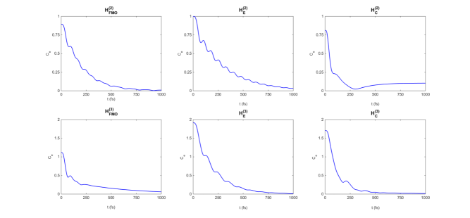
Figure 6: $C_{l_{1}}^{(e)}$ as a function of $t$ for $\hat{H}_{{\rm{FMO}}}^{(N)}$, $\hat{H}_{{\rm{\rm{E}}}}^{(N)}$ and $\hat{H}_{{\rm{C}}}^{(N)}$. The upper panel shows results for the dimer systems and the lower panel shows results for the trimer systems.

The efficiency maximized over $T$ and $t$, i.e., $F_{{\rm{OS,max}}}^{(\lambda,\tau)}$, is shown in Fig. 3 while the time dependence of the efficiency maximized over all environmental parameters, $F_{{\rm{OS,max}}}^{(t)}$, is shown in Fig. 4. It should be noted that in neither of the systems, the maximal efficiency shows a strong temperature dependence, why we omit showing the temperature dependence explicitly.

The local coherences in the site basis, $C_{l_{1},ij}^{(s)}$, are shown in Fig. 5 while the coherence in the exciton basis, $C_{l_{1}}^{(e)}$, is shown in Fig. 6.

The value of the maximal efficiency, $F_{{\rm{OS,max}}}$, the values of the environmental parameters and the time for which $F_{{\rm{OS,max}}}$ is achieved, and the corresponding value of non-Markovianity are given in Tab. 4 for the dimer systems and in Tab. 5 for the trimer systems. The time evolution of the trace distance of optimal state pairs, $D_{{\rm{OS,max}}}$, is shown in Fig. 7. The values of the environmental parameters and the corresponding value of non-Markovianity, but now for minimal efficiency, $F_{{\rm{OS,min}}}$, are shown in Tab. 6 (dimers) and Tab. 7 (trimers) for comparison.

Table 4: Maximal efficiency in the open dimer systems, $F_{{\rm{OS,max}}}$, environmental parameters and time for $F_{{\rm{OS,max}}}$, and corresponding values of non-Markovianity. For comparison, maximal efficiency in the closed system, $F_{{\rm{CS,max}}},$ and the efficiency in the long-time limit, $F_{{\rm{eq}}},$ are also shown.

	$F_{{\rm{OS,max}}}$	$\lambda_{{\rm{OS,max}}}\>({\rm{cm}^{-1})}$	$\tau_{{\rm{OS,max}}}\>({\rm{fs})}$	$T_{{\rm{OS,max}}}\>({\rm{K})}$	$t_{{\rm{OS,max}}}\>({\rm{fs})}$	$\mathcal{N}_{{\rm{OS,max}}}$	$F_{{\rm{CS,max}}}$	$F_{{\rm{eq}}}$
$\hat{H}_{{\rm{FMO}}}^{(2)}$	$0.83$	$20$	$50$	$250$	$72.5$	$0.045$	$0.89$	$0.61$
$\hat{H}_{{\rm{E}}}^{(2)}$	$0.91$	$20$	$50$	$250$	$77.5$	$0.11$	$1$	$0.71$
$\hat{H}_{{\rm{C}}}^{(2)}$	$0.84$	$220$	$50$	$250$	$1000$	$0.074$	$0.81$	$0.82$

Table 5: Maximal efficiency in the open trimer systems, $F_{{\rm{OS,max}}}$, environmental parameters and time for $F_{{\rm{OS,max}}}$, and corresponding values of non-Markovianity. For comparison, maximal efficiency in the closed system, $F_{{\rm{CS,max}}},$ and the efficiency in the long-time limit, $F_{{\rm{eq}}},$ are also shown.

	$F_{{\rm{OS,max}}}$	$\lambda_{{\rm{OS,max}}}\>({\rm{cm}^{-1})}$	$\tau_{{\rm{OS,max}}}\>({\rm{fs})}$	$T_{{\rm{OS,max}}}\>({\rm{K})}$	$t_{{\rm{OS,max}}}\>({\rm{fs})}$	$\mathcal{N}_{{\rm{OS,max}}}$	$F_{{\rm{CS,max}}}$	$F_{{\rm{eq}}}$
$\hat{H}_{{\rm{FMO}}}^{(3)}$	$0.76$	$80$	$50$	$250$	$1000$	$0.024$	$0.29$	$0.80$
$\hat{H}_{{\rm{E}}}^{(3)}$	$0.82$	$20$	$50$	$250$	$110$	$0.069$	$1$	$0.56$
$\hat{H}_{{\rm{C}}}^{(3)}$	$0.65$	$20$	$50$	$250$	$60$	$0.026$	$0.71$	$0.48$

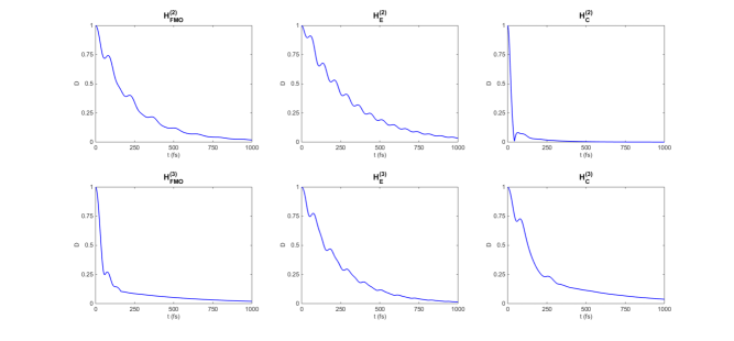
Figure 7: $D_{{\rm{OS,max}}}$ as a function of $t$ for $\hat{H}_{{\rm{FMO}}}^{(N)}$, $\hat{H}_{{\rm{E}}}^{(N)}$ and $\hat{H}_{{\rm{C}}}^{(N)}$. The upper panel shows results for the dimer systems and the lower panel shows results for the trimer systems.

Table 6: Minimal efficiency in the open dimer systems, $F_{{\rm{OS,min}}}$, environmental parameters for $F_{{\rm{OS,min}}}$ and corresponding values of non-Markovianity.

	$F_{{\rm{OS,min}}}$	$\lambda_{{\rm{OS,min}}}\>({\rm{cm}^{-1})}$	$\tau_{{\rm{OS,min}}}\>({\rm{fs})}$	$T_{{\rm{OS,min}}}\>({\rm{K}})$	$\mathcal{N_{{\rm{OS,min}}}}$
$\hat{H}_{{\rm{FMO}}}^{(2)}$	$0.59$	$220$	$50$	$250$	$0.079$
$\hat{H}_{{\rm{E}}}^{(2)}$	$0.67$	$220$	$550$	$250$	$0.64$
$\hat{H}_{{\rm{C}}}^{(2)}$	$0.72$	$50$	$550$	$300$	$0.76$

Table 7: Minimal efficiency in the open trimer systems, $F_{{\rm{OS,min}}}$, environmental parameters for $F_{{\rm{OS,min}}}$ and corresponding values of non-Markovianity.

	$F_{{\rm{OS,min}}}$	$\lambda_{{\rm{OS,min}}}\>({\rm{cm}^{-1})}$	$\tau_{{\rm{OS,min}}}\>({\rm{fs})}$	$T_{{\rm{OS,min}}}\>({\rm{K}})$	$\mathcal{N_{{\rm{OS,min}}}}$
$\hat{H}_{{\rm{FMO}}}^{(3)}$	$0.48$	$20$	$550$	$250$	$0.50$
$\hat{H}_{{\rm{E}}}^{(3)}$	$0.51$	$220$	$550$	$300$	$0.37$
$\hat{H}_{{\rm{C}}}^{(3)}$	$0.54$	$220$	$550$	$250$	$0.30$

V.1 Dimer

As can be seen in Tab. 4, EET from site $1$ to $2$ in the systems with Hamiltonians $\hat{H}_{{\rm{FMO}}}^{(2)}$ and $\hat{H}_{{\rm{E}}}^{(2)}$ is optimal for the same values of the environmental parameters, which are the lowest possible in the defined regimes and hence yields EET close to a fully coherent evolution (due to the low value of $\lambda_{{\rm{OS,max}}}$). For the system $\hat{H}_{{\rm{C}}}^{(2)}$, the scenario is different. Here, $\lambda_{{\rm{OS,max}}}$ is as large as possible in the defined regime (the optimal environmental values for $T$ and $\tau$ coincide with $\hat{H}_{{\rm{FMO}}}^{(2)}$ and $\hat{H}_{{\rm{E}}}^{(2)}$) and should be associated with an incoherent evolution. We discuss the optimal environmental regimes for the different systems in more detail below.

• For the system with Hamiltonian $\hat{H}_{{\rm{FMO}}}^{(2)},$ $E_{2}>E_{1}$ and at equilibrium site $1$ will be the most populated. Hence, EET from site $1$ to site $2$ may benefit from an EET within the coherent regime since it could allow for quantum tunneling over the energy barrier between the sites. Indeed, from the numerical calculations it is found that $F_{{\rm{CS,max}}}\approx\frac{3}{2}F_{{\rm{eq}}}$, which confirms that the most important feature of the environment is to preserve coherence. In Fig. 5 it can be seen that a large amount of coherence between site $1$ and $2$ is built up on a short time scale. Fig. 6 reveals a monotonically decreasing, oscillating coherence in the exciton basis. A similar behavior can be seen for $D_{{\rm{OS,max}}}$ in Fig. 7.

• For the system with Hamiltonian $\hat{H}_{{\rm{E}}}^{(2)}$, $F_{{\rm{CS,max}}}=1$ (see Ref. (Bengtson and Sjöqvist, 2017)) and $E_{1}=E_{2}.$ In this case, $F_{{\rm{eq}}}=0.71$ and $F_{{\rm{OS,min}}}=0.67$ for $\lambda_{{\rm{OS,min}}}=220\>{\rm{cm}^{-1}}.$ Again, as in the case of $\hat{H}_{{\rm{FMO}}}^{(2)},$ the EET is favored by environmental interactions that preserve a coherent EET, which implies preservation of coherence in the site basis (see Fig. 5). Here, $C_{l_{1}}^{(e)}$ and $D_{{\rm{OS,max}}}$ follows the same pattern as for $\hat{H}_{{\rm{FMO}}}^{(2)}$.

• In the last dimer system, with system Hamiltonian $\hat{H}_{{\rm{C}}}^{(2)},$ the situation is different - as already noted - from $\hat{H}_{{\rm{FMO}}}^{(2)}$ and $\hat{H}_{{\rm{E}}}^{(2)}$, which can be seen in Tab. 4 and Fig. 4. Still, even though $F_{{\rm{OS,max}}}$ in this case (unlike the others) is achieved for a large value of $\lambda$ ($\lambda_{{\rm{OS,max}}}=220\>{\rm{cm}^{-1}}$) , the dependence on $\lambda$ is not very strong (see Fig. 3). From Tab. 4 it can further be seen that the EET can occur with approximately equal efficiency in the very coherent regime ($F_{{\rm{CS,max}}}=0.81$ ) as in the long time limit ($F_{{\rm{eq}}}=0.82$). Hence, efficient EET could be expected for either a small value of $\lambda$ or a small value of $\tau$. It should also be noted that $F_{{\rm{OS,max}}}$ ($0.84$) does not seem to approach $F_{{\rm{eq}}}$ in the long-time limit. In Ref. (Subaşi et al., 2012) it is shown that the Boltzmann population does not describe the system equilibrium when the system and the environment is strongly coupled, which might be the reason why $F_{{\rm{OS,max}}}$ is even higher than $F_{{\rm{eq}}}$ according to Eq. 6 in this case. The coherence in the exciton basis, as shown in Fig. 6, reveals that indeed does the system approach a steady state that differs from the Boltzmann state since the coherence approaches a stationary non-zero value. Another interesting feature of the system $\hat{H}_{{\rm{C}}}^{(2)}$ is that even though oscillations in the coherence in the exciton basis (which might indicate information back flow from the environment) are quenched at a time scale of less than $100$ ${\rm{fs}}$, the value of $\mathcal{N}_{{\rm{OS,max}}}$ is higher than for $\hat{H}_{{\rm{FMO}}}^{(2)}$. This despite that the coherence in the exciton basis is maintained for much longer in the latter case. The information backflow in $\hat{H}_{{\rm{C}}}^{(2)}$ consists of one single peak, arising from zero distinguishability, which can be seen in Fig. 7. Since non-Markovianity is zero when the initial states for example are chosen as $\hat{\rho}_{1}(0)=\ket{1}\bra{1}$ and $\hat{\rho}_{2}(0)=\ket{2}\bra{2}$, it also shows the necessity of using the non-Markovian measure in the way it is intended to and not only select one or a few pairs of initial states.

By comparing the values of $F_{{\rm{OS,max}}}$ for each system in Tab. 4 to the values of $F_{{\rm{OS,min}}}$ in Tab. 6 together with the corresponding values of non-Markovianity in each case, it can be seen that non-Markovianty is higher for environments corresponding to minimal efficiency in all three dimer systems. Hence it can be concluded that non-Markovianity does not seem to be a resource - in the sense that a higher value of non-Markovianity correlates with a higher EET efficiency - for efficient EET in these dimer systems. The results also indicate that, as could have been expected, $\tau$ is the parameter that mainly governs the amount of non-Markovianity.

V.2 Trimer

In the trimer case, EET from site $1$ to $3$ is optimal for the same values of the environmental parameters for both the system with Hamiltonian $\hat{H}_{{\rm{E}}}^{(3)}$ and the system with Hamiltonian $\hat{H}_{{\rm{C}}}^{(3)}$, which are the lowest possible in the defined regimes as can be seen in Tab. 5. Here, it is the system with Hamiltonian $\hat{H}_{{\rm{FMO}}}^{(3)}$ that is optimized in a less coherent regime than the other two systems. We discuss these results in more detail below.

• The values of the optimal environmental parameters for the system with Hamiltonian $\hat{H}_{{\rm{FMO}}}^{(3)}$ are such that $T_{{\rm{OS,max}}}$ and $\tau_{{\rm{OS,max}}}$ are the lowest possible, but $\lambda_{{\rm{OS,max}}}$ is in an intermediate regime ($80\>{\rm{cm^{-1}}})$. For this system, $F_{{\rm{CS,max}}}$ is very small ($0.29$) and consequently, $F_{{\rm{OS,min}}}$ is obtained at $\lambda_{{\rm{OS,min}}}=20\>{\rm{cm}^{-1}}$. In Fig. 3 it can be seen that for $\lambda>80\>{\rm{cm}^{-1}}$ the efficiency is also considerably reduced and in Tab. 5 it can be noted that $F_{{\rm{eq}}}>F_{{\rm{OS,max}}}$, i.e., the efficiency in the long-time limit is higher than the value achieved at optimized parameter values. Here seems to be a case where the time scale of EET comes into play. Reaching equilibrium population for an initial population of site $2$ could be expected to be a faster process than from site $1$ since $E_{2}>E_{1}>E_{3}$. Hence, EET may benefit from - at least partly - taking the route over site $2$. A mechanism where the excitation can be transferred from site $1$ to $2$, despite the energy barrier, is quantum tunneling, i.e., a coherent dynamics initially can transfer the excitation to site $2$ and then, from there, an energetic downhill funneling is most efficient to transfer the excitation to site $3$. In Fig. 5 it can be seen that a large amount of coherence is built up between site $1$ and $2$ on a short time scale. The maximum of EET efficiency (with respect to $\lambda$ and $\tau$), observed in Fig. 3 can be understood as an interplay between coherent dynamics to transfer the excitation from site $1$ to $2$ and quenching of the coherent dynamics when the population is located at site $2$ to break reversibility. In the given time frame, this seems to be the most efficient EET process for this system.

• The system with Hamiltonian $\hat{H}_{{\rm{E}}}^{(3)}$, with $F_{{\rm{CS,max}}}=1$, follows the same pattern as the corresponding system in the dimer case. Indeed are the values of the optimal environmental parameters as low as possible in the defined regime and provide a close-to-coherent EET dynamics.

• The last trimer system, with system Hamiltonian $\hat{H}_{{\rm{C}}}^{(3)}$, has a structure where $E_{1}>E_{3}>E_{2}$ and the energy barrier between site $2$ and $3$ is large. At the same time, the coupling between these two sites is very weak in comparison to the energy difference between them as well as to the coupling to site $1$. Equilibrium population naturally favors site $2$ over site $3$ and therefore $F_{{\rm{eq}}}$ is rather small ($0.48$). In the closed system however, $F_{{\rm{CS,max}}}=0.71$ and hence, this system benefits from a coherent EET dynamics.

The coherence in the exciton basis is monotonically decaying, more or less oscillating, for all trimer systems. For the system $\hat{H}_{{\rm{FMO}}}^{(3)}$, the pattern is initially similar to $\hat{H}_{{\rm{C}}}^{(2)}$and the other two trimer systems resembles $\hat{H}_{{\rm{\rm{FMO}}}}^{(2)}$ and $\hat{H}_{{\rm{E}}}^{(2)}$. Again, there is a similarity between the appearance of $C_{l_{1}}^{(e)}$ and $D_{{\rm{OS,max}}}$.

As in the dimer systems, there does not seem to be any indications that non-Markovianity would be a resource for efficient EET. By comparing $\mathcal{N}_{{\rm{OS,max}}}$ to $\mathcal{N}_{{\rm{OS,min}}}$ and the corresponding parameter values in Tabs. 5 and 7, the observation that a larger value of $\tau$ yields a larger value of $\mathcal{N}$ is confirmed.

VI Conclusions

Previous studies on environment-assisted quantum transport (ENAQT) in pigment-protein molecular aggregates (Qin et al., 2014; Plenio and Huelga, 2008; Caruso et al., 2009; Chin et al., 2010; Sinayskiy et al., 2012; Marais et al., 2013; Wu et al., 2010; Rebentrost et al., 2009a, b; Mohseni et al., 2008; Dijkstra and Tanimura, 2012; Shabani et al., 2012; Mohseni et al., 2014) have, among others, proposed the following mechanisms for an enhanced EET efficiency:

• The environment can suppress pathways not leading to an enhanced probability of finding the excitation on the end site.

• Strongly coupled vibrational modes in the environment can induce resonant energy transfer between two sites/excitons that in the static picture are non-resonant.

In particular it has been noted that for EET that is very inefficient in the coherent regime, as the EET from site $1$ to site $3$ in the FMO-complex monomer, the efficiency can be increased considerably by adding environmental effects. In this study, we do not aim to explain the exact mechanisms for ENAQT, but rather try to pin down some simple design principles (in terms of environmental properties) for how to achieve efficient EET in model pigment-protein molecular aggregates.

Our study indicates that the information about optimal environmental conditions for efficient EET is in the structure of the closed system Hamiltonian and in particular, the relationship between the site energies. In general, a strategy to predict the optimal environment for a system is to compare $F_{{\rm{CS,max}}}$ to $F_{{\rm{eq}}}$ of site $N$. If $F_{{\rm{CS,max}}}>F_{{\rm{eq}}}$, the most beneficial role of the environment to promote efficient EET is to preserve coherent EET dynamics (i.e., the system-environment coupling, $\lambda,$ should be small). If instead $F_{{\rm{eq}}}>F_{{\rm{CS,max}}}$, most efficient EET is achieved when the the system is driven towards equilibrium as fast as possible (i.e., the environmental time scale, $\tau$, should be small). In this study, efficient EET hence occurs in either of the two regimes “coherent dynamics” (as close to the closed system dynamics as possible) or “equilibrating” (as close to the equilibrium population as possible).

In terms of the system Hamiltonian parameter space, our results indicate that for systems where site $N$ is higher in energy than site $1$, the EET benefits from quantum tunneling between the sites and hence requires a dynamics within the coherent regime. The same is true for the system Hamiltonians where $E_{N}=E_{1}.$ In such a case, the most important design principle is to create an environment that allows for coherent EET dynamics to persist, i.e., the system should be weakly coupled to the environment. The environmental time scale is less important. If instead $E_{1}>E_{N}$, the system is favoring a fast return to equilibrium where $E_{N}$ obviously is more populated than $E_{1}$. Here, the environmental time scale should be designed to be as small as possible and the coupling strength between the system and the environment is of less importance. Still, depending on the energy landscape of the other sites in the network as well as their intersite couplings, the time scale of equilibration might be beyond the given time frame. Hence, in reality the most efficient EET process might be a combination of coherent tunneling between sites and a downhill funneling from site to site. We believe that the EET in the system with Hamiltonian $\hat{H}_{{\rm{FMO}}}^{(3)}$ is an example of such a combined process.

Previous studies on non-Markovian effects in pigment-protein molecular aggregates have mainly connected the occurrence of non-Markovianity to a prolonged duration of coherence (Caruso et al., 2010; Chen et al., 2014; Thorwart et al., 2009). In (Rebentrost and Aspuru-Guzik, 2011) it is noted though that in a FMO complex monomer, maximal non-Markovianity is within the same environmental regime as optimal EET efficiency according to Ref. (Rebentrost et al., 2009a). The authors suggest that the role of non-Markovianity could be to preserve coherence, which could be of importance for the first EET route (site $1$, $2$ and $3$) since there is an energy barrier between site $1$ and $2$ (which might require quantum tunneling). Even though the important features of the system Hamiltonian parameter space for these three sites coincide with our trimer system with Hamiltonian $\hat{H}_{{\rm{FMO}}}^{(3)}$ (with only the exact parameter values differing), the dynamics will differ a bit due to the omission of the other four pigments in the FMO-complex monomer in our calculations. It should be noted that even though non-Markovianity is quantified by the same measure as in the present study, the maximization over initial states is ignored. This might affect the conclusion about the connection between non-Markovianity and EET efficiency. Indeed our study does not indicate a general connection between EET efficiency and non-Markovianity.

The parameter that seemingly affects the amount of non-Markovianity - and hence, the backflow of information from the environment to the system - the most, is the environmental time scale $(\tau$). The systems where $F_{{\rm{OS,max}}}$ is achieved in the coherent regime are not particularly sensitive to a potential backflow of information as accompanied with large values of $\tau$, but they do not seem to benefit from it either.

Another general feature worth noticing is that the pattern of the trace distance is very similar to the pattern of coherence in the exciton basis when $\lambda$ is small (see Figs. 6 and 7). This result suggests that a temporal increase of coherence in the exciton basis indeed may be interpreted as a backflow of information from the environment to the system and could possibly detect non-Markovian dynamics.

Lastly, our study shows the necessity of using the BLP-measure the way that it is intended to since a predefined choice of an initial state pair may give an arbitrary result.

References

- Breuer and Petruccione (2002) H.-P. Breuer and F. Petruccione, The theory of open quantum systems (Oxford University Press, 2002).
- Engel et al. (2007) G. S. Engel, T. R. Calhoun, E. L. Read, T.-K. Ahn, T. Mancal, Y.-C. Cheng, R. E. Blankenship, and G. R. Fleming, Nature 446, 782 (2007).
- Hayes et al. (2010) D. Hayes, G. Panitchayangkoon, K. A. Fransted, J. R. Caram, J. Wen, K. F. Freed, and G. S. Engel, New J. Phys. 12, 065042 (2010).
- Panitchayangkoon et al. (2010) G. Panitchayangkoon, D. Hayes, K. A. Fransted, J. R. Caram, E. Harel, J. Wen, R. E. Blankenship, and G. S. Engel, Proc. Natl. Acad. Sci. U.S.A. 107, 12766 (2010).
- Panitchayangkoon et al. (2011) G. Panitchayangkoon, D. V. Voronine, D. Abramavicius, J. R. Caram, N. H. Lewis, S. Mukamel, and G. S. Engel, Proc. Natl. Acad. Sci. U.S.A. 108, 20908 (2011).
- Chain and Arnon (1977) R. K. Chain and D. I. Arnon, Proc. Natl. Acad. Sci. U.S.A. 74, 3377 (1977).
- Qin et al. (2014) M. Qin, H. Z. Shen, X. L. Zhao, and X. X. Yi, Phys. Rev. E 90, 042140 (2014).
- Plenio and Huelga (2008) M. B. Plenio and S. F. Huelga, New J. Phys. 10, 113019 (2008).
- Caruso et al. (2009) F. Caruso, A. W. Chin, A. Datta, S. F. Huelga, and M. B. Plenio, J. Chem. Phys. 131, 105106 (2009).
- Chin et al. (2010) A. W. Chin, A. Datta, F. Caruso, S. F. Huelga, and M. B. Plenio, New J. Phys. 12, 065002 (2010).
- Sinayskiy et al. (2012) I. Sinayskiy, A. Marais, F. Petruccione, and A. Ekert, Phys. Rev. Lett. 108, 020602 (2012).
- Marais et al. (2013) A. Marais, I. Sinayskiy, A. Kay, F. Petruccione, and A. Ekert, New J. Phys. 15, 013038 (2013).
- Wu et al. (2010) J. Wu, F. Liu, Y. Shen, J. Cao, and R. J. Silbey, New. J. Phys. 12, 105012 (2010).
- Rebentrost et al. (2009a) P. Rebentrost, M. Mohseni, and A. Aspuru-Guzik, J. Phys. Chem. B 113, 9942 (2009a).
- Rebentrost et al. (2009b) P. Rebentrost, M. Mohseni, I. Kassal, S. Lloyd, and A. Aspuru-Guzik, New J. Phys. 11, 033003 (2009b).
- Mohseni et al. (2008) M. Mohseni, P. Rebentrost, S. Lloyd, and A. Aspuru-Guzik, J. Chem. Phys. 129, 174106 (2008).
- Dijkstra and Tanimura (2012) A. G. Dijkstra and Y. Tanimura, New J. Phys. 14, 073027 (2012).
- Shabani et al. (2012) A. Shabani, M. Mohseni, H. Rabitz, and S. Lloyd, Phys. Rev. E 86, 011915 (2012).
- Mohseni et al. (2014) M. Mohseni, A. Shabani, S. Lloyd, and H. Rabitz, J. Chem. Phys. 140, 035102 (2014).
- Tanimura and Kubo (1989a) Y. Tanimura and R. Kubo, J. Phys. Soc. Jpn. 58, 101 (1989a).
- Tanimura and Kubo (1989b) Y. Tanimura and R. Kubo, J. Phys. Soc. Jpn. 58, 1199 (1989b).
- Tanimura (1990) Y. Tanimura, Phys. Rev. A 41, 6676 (1990).
- Ishizaki and Fleming (2009a) A. Ishizaki and G. R. Fleming, J. Chem. Phys. 130, 234111 (2009a).
- Ishizaki and Fleming (2009b) A. Ishizaki and G. R. Fleming, Proc. Natl. Acad. Sci. U.S.A. 106, 17255 (2009b).
- Paz and Roncaglia (2008) J. P. Paz and A. J. Roncaglia, Phys. Rev. Lett. 100, 220401 (2008).
- Valido et al. (2013a) A. A. Valido, L. A. Correa, and D. Alonso, Phys. Rev. A 88, 012309 (2013a).
- Valido et al. (2013b) A. A. Valido, D. Alonso, and S. Kohler, Phys. Rev. A 88, 042303 (2013b).
- Bellomo et al. (2007) B. Bellomo, R. Lo Franco, and G. Compagno, Phys. Rev. Lett. 99, 160502 (2007).
- Huelga et al. (2012) S. F. Huelga, Á. Rivas, and M. B. Plenio, Phys. Rev. Lett. 108, 160402 (2012).
- Maniscalco et al. (2007) S. Maniscalco, S. Olivares, and M. G. A. Paris, Phys. Rev. A 75, 062119 (2007).
- Bylicka et al. (2014) B. Bylicka, D. Chruściński, and S. Maniscalco, Sci. Rep. 4, 5720 (2014).
- Caruso et al. (2014) F. Caruso, V. Giovannetti, C. Lupo, and S. Mancini, Rev. Mod. Phys. 86, 1203 (2014).
- Laine et al. (2014) E.-M. Laine, H.-P. Breuer, and J. Piilo, Sci. Rep. 4, 4620 (2014).
- Liu et al. (2013) B.-H. Liu, D.-Y. Cao, Y.-F. Huang, C.-F. Li, G.-C. Guo, E.-M. Laine, H.-P. Breuer, and J. Piilo, Sci. Rep. 3, 1781 (2013).
- Thorwart et al. (2009) M. Thorwart, J. Eckel, J. H. Reina, P. Nalbach, and S. Weiss, Chem. Phys. Lett. 478, 234 (2009).
- Chen et al. (2014) H.-B. Chen, J.-Y. Lien, H. Chi-Chuan, and Y.-N. Chen, Phys. Rev. E 89, 042147 (2014).
- Rebentrost and Aspuru-Guzik (2011) P. Rebentrost and A. Aspuru-Guzik, J. Chem. Phys. 134, 101103 (2011).
- Mujica-Martinez et al. (2013) C. A. Mujica-Martinez, P. Nalbach, and M. Thorwart, Phys. Rev. E 88, 062719 (2013).
- Breuer et al. (2009) H.-P. Breuer, E.-M. Laine, and J. Piilo, Phys. Rev. Lett. 103, 210401 (2009).
- Rivas et al. (2010) Á. Rivas, S. F. Huelga, and M. B. Plenio, Phys. Rev. Lett. 105, 050403 (2010).
- Rajogopal et al. (2010) A. K. Rajogopal, A. R. Usha Devi, and R. W. Rendell, Phys. Rev. A 82, 042107 (2010).
- Baumgratz et al. (2014) T. Baumgratz, M. Cramer, and M. B. Plenio, Phys. Rev. Lett. 113, 140401 (2014).
- Renger et al. (2001) T. Renger, V. May, and O. Kühn, Phys. Rep. 343, 137 (2001).
- Fenna et al. (1974) R. E. Fenna, B. W. Matthews, J. M. Olson, and E. K. Shaw, J. Mol. Biol. 84, 231 (1974).
- Caruso et al. (2010) S. Caruso, A. W. Chin, A. Datta, S. F. Huelga, and M. B. Plenio, Phys. Rev. A 81, 062346 (2010).
- Sarovar et al. (2010) M. Sarovar, A. Ishizaki, G. R. Fleming, and K. B. Whaley, Nat. Phys. 6, 462 (2010).
- Fassioli and Olaya-Castro (2010) F. Fassioli and A. Olaya-Castro, New J. Phys. 12, 085006 (2010).
- Baker and Habershon (2015) L. A. Baker and S. Habershon, J. Chem. Phys. 143, 105101 (2015).
- Chen et al. (2013) G.-Y. Chen, N. Lambert, C.-M. Li, Y.-N. Chen, and F. Nori, Phys. Rev. E 88, 032120 (2013).
- Shabani et al. (2014) A. Shabani, M. Mohseni, H. Rabitz, and S. Lloyd, Phys. Rev. E 89, 042706 (2014).
- Wu et al. (2012) J. Wu, F. Liu, J. Ma, R. J. Silbey, and J. Cao, J. Chem. Phys. 137, 174111 (2012).
- Bengtson and Sjöqvist (2017) C. Bengtson and E. Sjöqvist, New J. Phys. 19, 113015 (2017).
- Nielsen and Chuang (2010) M. A. Nielsen and I. L. Chuang, Quantum Computation and Quantum Information (Cambridge University Press, Cambridge, England, 2010).
- Ruskai (1994) M. B. Ruskai, Rev. Math. Phys. 6, 1147 (1994).
- Wißmann et al. (2012) S. Wißmann, A. Karlsson, E.-M. Laine, J. Piilo, and H.-P. Breuer, Phys. Rev. A 86, 062108 (2012).
- Bronzan (1988) J. B. Bronzan, Phys. Rev. D 38, 1994 (1988).
- Wootters (1998) W. K. Wootters, Phys. Rev. Lett. 80, 2245 (1998).
- Subaşi et al. (2012) Y. Subaşi, C. H. Fleming, J. M. Taylor, and B. L. Hu, Phys. Rev. E 86, 061132 (2012).