Kramers-Kronig relations and the properties of conductivity and permittivity in heterogeneous media

Abstract

The macroscopic electric permittivity of a given medium may depend on frequency, but this frequency dependence cannot be arbitrary, its real and imaginary parts are related by the well-known Kramers-Kronig relations. Here, we show that an analogous paradigm applies to the macroscopic electric conductivity. If the causality principle is taken into account, there exists Kramers-Kronig relations for conductivity, which are mathematically equivalent to the Hilbert transform. These relations impose strong constraints that models of heterogeneous media should satisfy to have a physically plausible frequency dependence of the conductivity and permittivity. We illustrate these relations and constraints by a few examples of known physical media. These extended relations constitute important constraints to test the consistency of past and future experimental measurements of the electric properties of heterogeneous media.

1 Introduction

The theory of electromagnetism can be applied to complex media like inhomogeneous materials or biological tissue. A first approach to such media is to explicitly consider their microscopic structure, and the associated variations of electric conductivity or permittivity, but this approach requires a detailed mapping of these electric parameters and include this in detailed simulations. Another approach is to use a mean-field electromagnetic theory by considering scales larger than the typical scales of inhomogeneities in the medium. In this case, the mean-field theory relates to macroscopic measurements of conductivity and permittivity. For example, in neural tissue, macroscopic measurements of these quantities were done in a number of studies [2, 3, 4, 5] who measured the frequency dependence of electric parameters in different conditions (reviewed in ref. [6]). Theoretical work showed that this frequency dependence can be accounted by physical phenomena such as ionic diffusion or cell polarization [9, 10]. In the present paper, we investigate the relations between the apparent macroscopic conductivity and permittivity and show that they cannot take arbitrary values but are strongly constrained to be consistent with Maxwell’s theory of electromagnetism.

An important aspect of the equations of electromagnetism when applied to media with a given electric permittivity $\varepsilon(\vec{r},t)$, is that the real $\varepsilon^{\prime}$ and imaginary $\varepsilon^{\prime\prime}$ parts of the complex Fourier transform of $\varepsilon(\vec{r},\omega)$ cannot take independent values, but they are linked together by a set of mathematical relations called Kramers-Kronig relations [11, 12, 13]. These relations are a direct consequence of the principle of causality, namely that the future cannot influence the past [11], and were shown to be equivalent to the Hilbert transform in a perfect dielectric [14, 15].

Here, we will re-examine these Kramers-Kronig relations and their equivalence to Hilbert transforms in heterogeneous media. The goal is to determine the constraints that the frequency dependence of electric conductivity and permittivity must satisfy. We will also consider the application of this formalism to a few concrete examples.

2 Theory

We begin by setting the framework of the present study, by outlining the electromagnetic theory used here, and how to apply it to heterogeneous media. We next consider the Kramers-Kronig relations within this framework.

2.1 General framework

To derive a formalism applicable to heterogeneous media, we consider linear media within the electric quasi-static approximation in mean-field[16, 17], which corresponds to a physical situation where electromagnetic induction can be neglected. This is the case for neural tissue, where we have an excellent approximation of the electric field if we assume

$$\left\{\begin{array}[]{cccc}\nabla\cdot\bf{\vec{D}}&=&~{}~{}~{}\bf{\rho^{free}}\\ \nabla\times\bf{\vec{E}}&=&0\end{array}\right.$$ (1)

where the fields $\bf{\vec{E}},~{}\bf{\vec{D}},~{}\bf{\rho^{free}}$ are mean-fields over a base volume $\mathcal{V}$ [10]. By definition, we have $\textbf{X}=<X>{\big{|}}_{\mathcal{V}}$ .

In this approximation of the Maxwell-Heaviside equations, the electric field and magnetic induction are such that $\parallel\bf{\vec{E}}\parallel~{}>>~{}c\parallel\bf{\vec{B}}\parallel$ where $c$ is the velocity of electromagnetic waves [16]. Thus, in this approximation, we can calculate $\vec{\bf{E}}$ independently of $\vec{\bf{B}}$ and $\vec{\bf{H}}$ if we know the linking equation between $\vec{\bf{D}}$ and $\vec{\bf{E}}$.

On the other hand, the link between the electric displacement field and magnetic field always hold because we have

$$\left\{\begin{array}[]{cccc}\nabla\cdot\vec{\bf{B}}&=&0\\ \nabla\times\vec{\bf{B}}&=&\mu_{o}~{}[\vec{\bf{j}}^{free}+\frac{\partial\vec{\bf{D}}}{\partial t}]\end{array}\right.$$ (2)

where $\mu_{o}$ is the magnetic permeability of vacuum. We do not consider here the situation where this permeability would be different from vacuum, which normally should be a good approximation because of the absence of large amounts of ferromagnetic, paramagnetic or diamagnetic materials in neural tissue.

Moreover, if we restrict to isotropic media (when the inhomogeneity of the medium similarly affects all directions), we have:

$$\left\{\begin{array}[]{ccccc}\vec{\bf{D}}(\vec{r},t)&=&\int_{-\infty}^{+\infty}\bf{\varepsilon}(\vec{r},\tau)~{}\vec{\bf{E}}(\vec{r},t-t)~{}d\tau&(a)\\ \\ \vec{\bf{j}}^{free}(\vec{r},t)&=&\int_{-\infty}^{+\infty}\bf{\sigma}_{e}(\vec{r},\tau)~{}\vec{\bf{E}}(\vec{r},t-\tau)~{}d\tau&(b)\end{array}\right.$$ (3)

where $\bf{\varepsilon}(\vec{r},t)$ and $\bf{\sigma}_{e}(\vec{r},t)$ are real-valued functions.

This formalism applies to neural tissue, which can be considered as an heterogeneous isotropic medium within a mean-field context, when the base volume is sufficiently large ($>1~{}\mu m^{3}$; see ref. [10]). The linking equations imply that the values of $\vec{\bf{D}}$ and $\vec{\bf{j}}^{~{}free}$ at a given time depend on the past values of the electric field in general, which can be seen as a kind of “memory”. The only way to avoid such a memory is to assume $\bf{\sigma}_{e}(\vec{r},t)=\bf{\sigma}_{c}(\vec{r})~{}\delta(t)$ and $\bf{\varepsilon}(\vec{r},t)=\bf{\varepsilon}_{c}(\vec{r})~{}\delta(t)$ where $\bf{\sigma}_{c}$ et $\bf{\varepsilon}_{c}$ are not time-dependent. Note that such a memory is equivalent to having a frequency dependence of the electric permittivity and/or conductivity, when we formulate the problem in Fourier frequency space. In this case, the relations (3) imply $\vec{\bf{D}}(\vec{r},\omega)=\bf{\varepsilon}(\vec{r},\omega)\vec{\bf{E}}(\vec{r},\omega)$ et $\vec{\bf{j}}(\vec{r},\omega)=\bf{\sigma}_{e}(\vec{r},\omega)\vec{\bf{E}}(\vec{r},\omega)$.

Finally, recalling that $\nabla\cdot\vec{\bf{D}}$ allows us to calculate the free charge density in a region $\mathcal{D}$, we have:

$$\bf{Q}^{free}(t)=\iiint\limits_{\mathcal{D}}\nabla\cdot\vec{\bf{D}}~{}(\vec{r},t)~{}dxdydz$$ (4)

The electric permittivity $\varepsilon$ measures the amount of free charges in a given region. The higher the density, the larger the permittivity.

2.2 Electric conductivity and permittivity in a mean-field model of isotropic media

In the following, we will re-examine the Kramers-Kronig relations in the case of an heterogeneous and conductive medium, where the electric field is time dependent. In a first step, we show that the Kramers-Kronig relations are equivalents to the Hilbert transform if we apply them to $\omega\bf{\varepsilon}(\vec{r},\omega)$ instead of $\bf{\varepsilon}(\vec{r},\omega)$. In a second step, we show that we have the same relations for the conductivity $\bf{\sigma}_{e}$.

2.2.1 General expression for the absolute electric permittivity

According to relations (3), the electric displacement field $\vec{\bf{D}}$ is linked to the resulting electric field $\vec{\bf{E}}$ by a convolution integral:

$$\vec{\bf{D}}(\vec{r},t)=\int_{-\infty}^{+\infty}\bf{\varepsilon}(\vec{r},\tau)~{}\vec{\bf{E}}(\vec{x},t-\tau)~{}d\tau=\int_{-\infty}^{+\infty}\bf{\varepsilon}(\vec{x},t-\tau)~{}\vec{\bf{E}}(\vec{r},\tau)~{}d\tau$$ (5)

However, we must also assume that $\bf{\varepsilon}(\vec{x},t)=0$ when $\tau<0$ because the future cannot influence the past (causality principle). Thus, we can write

$$\vec{\bf{D}}(\vec{r},t)=\int_{0^{-}}^{+\infty}\bf{\varepsilon}(\vec{r},\tau)~{}\vec{E}(\vec{r},t-\tau)~{}d\tau$$ (6)

which is always valid in a plausible physical system.

Moreover, in general, we can write

$$\bf{\varepsilon}(\vec{r},t)=\varepsilon_{o}[\delta(t)+\bf{\chi}(\vec{r},t)]$$ (7)

which is always valid because $\bf{\chi}$ is an arbitrary function (or distribution). The parameter $\varepsilon_{o}=8.875\times 10^{-12}~{}F/m$ is the vacuum permittivity and $\bf{\chi}$ is the electric susceptibility expressed in temporal space. $\chi$ measures the amount of free charges induced by applying an electric field in the medium. Note that this phenomenon will be necessarily present in a heterogeneous medium such as neural tissue because we have charge accumulation in membranes when applied to an electric field. Note that the phenomenon of charge induction can change the law of attenuation with distance, as shown before [18].

Thus, we can write

$$\vec{\bf{D}}~{}(\vec{r},t)=\bf{\varepsilon}_{o}\int_{0}^{+\infty}[\delta(t)+\bf{\chi}(\vec{x},\tau)]~{}\vec{\bf{E}}(\vec{r},t-\tau)~{}d\tau=\varepsilon_{o}\vec{\bf{E}}+\int_{0}^{+\infty}\varepsilon_{o}\bf{\chi}(\vec{r},\tau)~{}\vec{\bf{E}}(\vec{r},t-\tau)~{}d\tau~{}~{}.$$ (8)

It follows that, if the Fourier transform relative to $\omega=2\pi\nu$ exists, then we have

$$\vec{\bf{D}}~{}(\vec{r},\omega)=\varepsilon_{o}~{}[1+\bf{\chi}(\vec{x},\omega)]~{}\vec{\bf{E}}(\vec{r},\omega)=\bf{\varepsilon}(\vec{r},\omega)~{}\vec{\bf{E}}(\vec{r},\omega)$$ (9)

where

$$\bf{\varepsilon}(\vec{r},\omega)=\varepsilon_{o}~{}{\Big{[}}1+\int_{~{}0}^{+\infty}\bf{\chi}(\vec{x},\tau)~{}e^{-i\omega\tau}d\tau~{}{\Big{]}}$$ (10)

We see that the electric permittivity in Fourier frequency space is in general a complex function, and its variation with respect to that of vacuum is such that

$$\bar{\Delta}\bf{\varepsilon}=\bf{\varepsilon}-\varepsilon_{o}=\int_{~{}0}^{+\infty}\varepsilon_{o}\bf{\chi}(\vec{x},\tau)~{}e^{-i\omega\tau}d\tau~{}.$$ (11)

The latter equation implies that we have $\bar{\Delta}\varepsilon=0$ when $\omega\rightarrow\infty$. Thus, the permittivity tends to that of vacuum when the frequency tends to infinity, which is in good agreement with experimental measurements. The real part of $\bar{\Delta}\bf{\varepsilon}(\omega)$ is an even function relative to the frequency $\omega$ and its imaginary part is an odd function because $\varepsilon_{o}\bf{\chi}(t)$ is a real function.

2.2.2 Analytic continuation of $\omega\varepsilon$ and the Kramers-Kronig or Hilbert transform

We have shown that the imaginary part of $\bar{\Delta}\bf{\varepsilon}(\vec{r},\omega)$ in Fourier frequency space must be odd and that the real part must be even if we want the system to be physically plausible. Moreover, it was shown that the real and imaginary parts of permittivity are linked by the Kramers-Kronig relations. However, we will develop this transform for $\omega~{}\bar{\Delta}\varepsilon(\vec{r},\omega)$ instead of $\bar{\Delta}\varepsilon(\vec{r},\omega)$ to make the formalism more uniform between conductivity and permittivity.

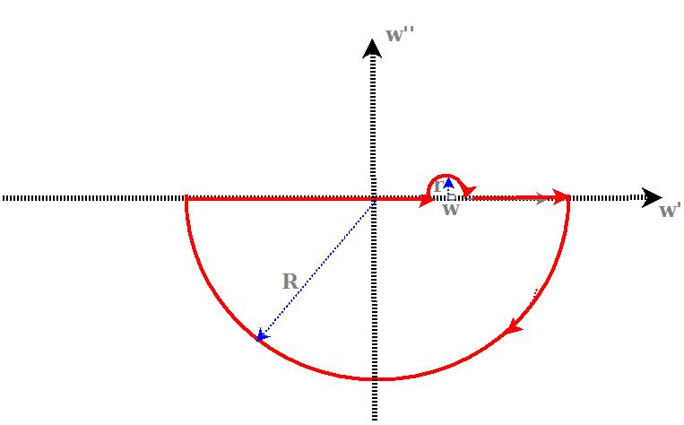
Figure 1: Illustration of the integration path in Region $\mathbb{P}$. The singular point $\omega_{a}=\omega$ is on the real segment inside the half circle indicated. If $r\rightarrow 0$ and $R\rightarrow\infty$, then applying the Cauchy integral gives the Hilbert transform.

According to expression (11), we have

$$\omega~{}\bar{\Delta}\bf{\varepsilon}=\int_{~{}0}^{+\infty}\omega~{}\varepsilon_{o}\bf{\chi}(\vec{x},\tau)~{}e^{-i\omega\tau}d\tau~{}$$ (12)

If we analytically continue the real frequency $\omega$ over the complex plane by setting $\omega=\omega^{\prime}+i\omega^{\prime\prime}$ then the last integral becomes

$$\int_{0}^{+\infty}\varepsilon_{o}\chi(\vec{r},\tau)~{}\omega e^{-i\omega\tau}d\tau~{}=\lim\limits_{\delta\rightarrow 0}\int_{\delta}^{1/\delta}\varepsilon_{o}~{}\bf{\chi}(\vec{r},\tau)~{}~{}[~{}\omega^{\prime}+i~{}(\omega^{\prime\prime}-\delta)~{}]~{}e^{-i\omega^{\prime}\tau}e^{(\omega^{\prime\prime}-\delta)\tau}~{}d\tau$$ (13)

where $\delta>0$. The last integral converges when $\omega^{\prime\prime}\leq 0$ and tends to zero when $\omega^{\prime\prime}\rightarrow-\infty$. It diverges when $\omega^{\prime\prime}>0$. Note that it is because we have applied the causality principle that the integral can converge for $\omega^{\prime\prime}<0$; omitting causality would prevent convergence because one would need to integrate between $-\infty$ and $+\infty$ (see Eq. 5).

Thus, the causality principle has the consequence that the function $\omega\bar{\Delta}\varepsilon$ is holomorphic in the complex inferior half-plane, as well as on the real axis. If we call this Region $\mathcal{P}$ and apply the Cauchy integral of a holomorphic function, which gives

$$\omega~{}\bar{\Delta}\bf{\varepsilon}(\vec{r},\omega)=\frac{1}{2\pi i}\oint\frac{\omega_{a}~{}\bar{\Delta}\bf{\varepsilon}(\vec{r},\omega_{a})}{\omega_{a}-\omega}d\omega_{a}$$ (14)

if the path is closed within Region $\mathcal{P}$, and if all points in this path are all situated at a finite distance from the origin. Note that, under this constraint, the function in the integral has only one singular point at $\omega_{a}=\omega$ because $\omega\bar{\Delta}\varepsilon$ is a holomorphic function inside $\mathcal{P}$. This is not the case for $\bar{\Delta}\bf{\varepsilon}$ in a conductive medium.

An interesting choice of path is a clockwise along the real axis, going around the singularity $\omega_{a}=\omega$ along a half-circle of radius $\delta$ and a large half-circle of radius $R=1/\delta$ (see Fig. 1). In this case, there is only the principal value of the integral on the real axis, and we can write

$$\omega~{}\bar{\Delta}\bf{\varepsilon}(\vec{r},\omega)=-\frac{1}{\pi i}\fint_{-\infty}^{+\infty}\frac{\omega_{a}~{}\bar{\Delta}\bf{\varepsilon}(\vec{r},\omega)}{\omega_{a}-\omega}d\omega_{a}$$ (15)

For $\omega_{a}\in\mathbb{R}$ and $|\omega_{a}|\rightarrow\infty$, we have $|\omega_{a}~{}\bar{\Delta}\bf{\varepsilon}(\vec{r},\omega)|\rightarrow 0$. Note that this condition is equivalent to postulate that $|\bar{\Delta}\bf{\varepsilon}(\vec{r},\omega_{a})|$ tends to 0 faster than $1/\omega_{a}$ when frequency tends to infinity. This insures that the integral in Eq. (15) converges. This is obtained because for $R\rightarrow\infty$ ($\delta\rightarrow 0$), the integral over the large circle is zero (see Eq. 10) while the integral over the small circle is equal to $-\omega~{}\bar{\Delta}\varepsilon(\vec{r},\omega)/2$ when $\delta\rightarrow 0$ (see Fig. 1). We note the principal part of the integral by $\fint$

We can separate the real and imaginary parts of $\omega~{}\bar{\Delta}\bf{\varepsilon}(\vec{r},\omega)$, leading to

$$\left\{\begin{array}[]{ccccc}\omega~{}\bar{\Delta}\bf{\varepsilon}^{\prime\prime}(\vec{r},\omega)=\mathcal{H}~{}(\omega~{}\bar{\Delta}\varepsilon^{\prime})=\frac{1}{\pi}\fint_{-\infty}^{+\infty}\frac{\omega_{a}~{}\bar{\Delta}\varepsilon^{\prime}(\vec{r},\omega_{a})}{\omega_{a}-\omega}d\omega_{a}&(a)\\ \\ \omega~{}\bar{\Delta}\varepsilon^{\prime}(\vec{r},\omega)=-\mathcal{H}~{}(\omega~{}\bar{\Delta}\varepsilon^{\prime\prime})=-\frac{1}{\pi}\fint_{-\infty}^{+\infty}\frac{\omega_{a}~{}\bar{\Delta}\varepsilon^{\prime\prime}.(\vec{r},\omega_{a})}{\omega_{a}-\omega}d\omega_{a}&(b)\end{array}\right.$$ (16)

Note that Eqs. (16a) and (16b) are of opposite sign as the Kramers-Kronig relations as presented by Landau & Lifshitz [11] and Forster & Schwan [13]. The reason for this difference is that our analytic continuation of the electric parameters are holomorphic in the negative half-plane, instead of the positive half-plane [14].

Consequently, the real and imaginary parts of $\omega\bar{\Delta}\varepsilon(\vec{r},\omega)$ are linked by the Hilbert transform. To calculate the real part from the knowledge of the imaginary part, one can apply the inverse Hilbert transform, while the direct transform is used to calculate the imaginary part from the real part. Note that this transform is totally equivalent to the Kramers-Kronig relations

Finally, we can write

$$\omega~{}\bar{\Delta}\bf{\varepsilon}=\omega~{}\bar{\Delta}\bf{\varepsilon}^{\prime}+i~{}\mathcal{H}[\omega\bar{\Delta}\varepsilon^{\prime}]=-\mathcal{H}[\omega~{}\bar{\Delta}\bf{\varepsilon}^{\prime\prime}]+i~{}\omega\bar{\Delta}\varepsilon^{\prime\prime}$$ (17)

We can see that the phase $\phi$ of $\omega~{}\bar{\Delta}\bf{\varepsilon}$ is such that we have: $tan(\phi)=\frac{\mathcal{H}[\omega\bar{\Delta}\varepsilon^{\prime}]}{\omega~{}\bar{\Delta}\bf{\varepsilon}^{\prime}}=-\frac{\omega\bar{\Delta}\varepsilon^{\prime\prime}}{\mathcal{H}[\omega~{}\bar{\Delta}\bf{\varepsilon}^{\prime\prime}]}$.

Thus, the phase is completely determined when either the real or imaginary part of $\omega~{}\bar{\Delta}\bf{\varepsilon}$ is known.

2.3 Electric conductivity within the quasi-static approximation

We now consider the temporal and frequency dependence of the electric conductivity in linear media within the electric quasi-static approximation. In the first section below, we review the constraints that must be satisfied in Fourier frequency space on the electric conductivity to simulate a physically plausible system. We show that the electric conductivity also obeys to a Hilbert transform, similar to that shown above for $\omega\bar{\Delta}\varepsilon$.

2.3.1 Electric conductivity and free-charge current in linear electromagnetism

It is well known that the most general relation between the free-charge current density $\vec{\bf{j}}^{free}(\vec{r},t)$ and the electric field $\vec{\bf{E}}(\vec{r},t)$ in linear electromagnetism is given by the convolution integral:

$$\vec{\bf{j}}^{free}(\vec{x},t)=\int_{-\infty}^{+\infty}\bf{\sigma}_{e}(\vec{r},t-\tau)~{}~{}\vec{\bf{E}}(\vec{r},\tau)~{}d\tau=\int_{-\infty}^{+\infty}\sigma_{e}(\vec{x},\tau)~{}~{}\vec{E}(\vec{x},t-\tau)~{}d\tau$$ (18)

where $\bf{\sigma}_{e}\geq 0$  Expression (1) can be written as:

$$\vec{\bf{j}}^{free}(\vec{r},\omega)=\bf{\sigma}_{e}(\vec{r},\omega)~{}~{}\vec{\bf{E}}(\vec{r},\omega)$$ (19)

in Fourier frequency space. Here, the convolution in temporal space corresponds to a simple product in frequency space. Note that the function $\bf{\sigma}_{e}(\vec{r},\omega)$ depends on the value of the electric field when the relation between the current density and eclectic field is nonlinear, but this dependence vanishes if the system is linear.

Finally, Ohm’s law corresponds to the simplest model expressed by Eqs. (17, 18). In this particular case, we have $\bf{\sigma}_{e}(\vec{x},t-\tau)=\bf{\sigma}(\vec{x})~{}\delta(t-\tau)$ where $\bf{\sigma}$ does not depend on time. $\delta$ is the Dirac distribution. This law corresponds to an idealized physical system without memory (see Section 2), were the work produced by the electric field on the free charges dissipates almost instantaneously in the system. Note we also have in this case $\vec{\bf{j}}^{free}(\vec{r},t)=\bf{\sigma}(\vec{r})~{}\vec{\bf{E}}(\vec{r},t)$ in temporal space, and we have a similar relation $\vec{\bf{j}}^{free}(\vec{r},\omega)=\bf{\sigma}(\vec{r})~{}\vec{\bf{E}}(\vec{r},\omega)$ in frequency space. Thus, we have the same algebraic relation between $\vec{\bf{j}}^{free}$ and $\vec{\bf{E}}$ in both spaces.

2.3.2 Constraints imposed by the causality principle

To be physically plausible, a system must obey the causality principle. This principle determines a constraint on the relation between the free-charge current density $\vec{\bf{j}}^{free}$ and the electric field $\vec{\bf{E}}$ (within the linear electromagnetic theory). According to this principle, the future cannot influence the past, and thus we can write that, at a given time $t$, $\vec{\bf{j}}^{free}$ and $\vec{\bf{E}}$ are related as

$$\vec{\bf{j}}^{free}(\vec{r},t)=\int_{0}^{+\infty}\bf{\sigma}_{e}(\vec{r},\tau)~{}~{}\vec{\bf{E}}(\vec{r},t-\tau)~{}d\tau$$ (20)

because the values of the electric field at times greater than $t$ cannot influence the current density at time $t$. Note that this is equivalent to assume that $\bf{\sigma}_{e}(\vec{r},\tau)=0$ when $\tau<0$ in Eq. (19). This constraint is general and must be included in all mathematical models of conductivity to be physically plausible.

2.3.3 Electrical conductivity in a heterogeneous medium

We now consider the case of a heterogeneous medium composed of different cells and various processes immersed in a conductive fluid, such that the distance between different elements $\delta_{c}$ is always greater than zero. We also assume that the electric conductivity of this medium tends asymptotically to $\bf{\sigma}_{\infty}(\vec{r},t)$ when the frequency $\nu$ tends to infinity. For high frequencies, there is a portion of free charges which does not meet any process, because their mean displacement becomes smaller than $\delta_{c}$. However, for sufficiently low frequencies, the presence of cells will impact all free charges, and the conductivity will be affected and will be different as that of high frequencies. Thus, the conductivity of a heterogeneous medium will necessarily be frequency dependent within some frequency range.

This intuitive explanation can be formulated more quantitatively. The electric conductivity can be expressed as

$$\bf{\sigma}_{e}(\vec{r},t)=\bf{\sigma}_{\infty}(\vec{r},t)[1+\bar{\Delta}_{e}(\vec{r},t)]$$ (21)

where $\bar{\Delta}_{e}(\vec{r},t)\neq 0$. It follows that Expression (5) can be written as

$$\vec{j}^{free}(\vec{r},t)=~{}~{}\int_{0}^{+\infty}\sigma_{\infty}(\vec{x},\tau)~{}~{}[~{}1+\bar{\Delta}_{e}(\vec{x},\tau)~{}~{}]~{}~{}\vec{E}(\vec{x},t-\tau)~{}d\tau~{}$$ (22)

Taking the Fourier transform, we obtain

$$\vec{\bf{j}}^{free}(\vec{r},\omega)={\Big{[}}~{}~{}\bf{\sigma}_{\infty}(\vec{r},\omega)+\int_{0}^{+\infty}\bf{\sigma}_{\infty}(\vec{r},\tau)~{}~{}\bar{\Delta}_{e}(\vec{r},\tau)~{}e^{-i\omega\tau}~{}d\tau~{}{\Big{]}}~{}~{}\vec{\bf{E}}(\vec{r},\omega)$$ (23)

Thus, we can write

$$\bf{\sigma}_{e}(\vec{r},\omega)=\bf{\sigma}_{\infty}(\vec{r},\omega)+\int_{0}^{+\infty}\bf{\sigma}_{\infty}(\vec{r},\tau)~{}~{}\bar{\Delta}_{e}(\vec{r},\tau)~{}~{}e^{-i\omega\tau}~{}d\tau$$ (24)

where the function $\bf{\sigma}_{\infty}(\vec{r},\tau)\bar{\Delta}_{e}(\vec{r},\tau)$ is such that the integral in Expression (24) tends to zero when $\omega\rightarrow\infty$. Thus, $\bf{\sigma}_{e}(\vec{r},\omega\rightarrow\infty)$ tends to $\bf{\sigma}_{\infty}(\vec{r},\omega)$. Note that the integral in the righthand side converges because it is the Fourier transform of $\bar{\Delta}\bf{\sigma}_{e}=\bf{\sigma}_{e}-\bf{\sigma}_{\infty}$.

2.3.4 Similar relations between $\omega\bar{\Delta}\bf{\varepsilon}$ and $\bar{\Delta}\bf{\sigma}_{e}$

We know that the imaginary part of $\bar{\Delta}\bf{\sigma}_{e}$ in frequency space is an odd function, while the real part is even, if the model is physically plausible because the time-dependent conductivity is a real function. However, these parts could still be independent of each-other. We now show that if we apply the causality principle, the imaginary part of $\bar{\Delta}\bf{\sigma}_{e}$ (in frequency space) is completely determined by its real part, via a Hilbert transform, exactly like $\omega\bar{\Delta}\bf{\varepsilon}$.

If we analytically continue the frequency $\omega$ over the complex plane by taking $\omega=\omega^{\prime}+i\omega^{\prime\prime}$, then the integral in Expression (23) becomes

$$\int_{0}^{+\infty}\bf{\sigma}_{\infty}(\vec{r},\tau)\bar{\Delta}_{e}(\vec{r},\tau)~{}~{}e^{-i\omega\tau}~{}d\tau=\lim\limits_{\delta\rightarrow 0}\int_{\delta}^{1/\delta}\sigma_{\infty}(\vec{r},\tau)\bar{\Delta}_{e}(\vec{r},\tau)~{}~{}e^{-i\omega^{\prime}\tau}e^{(\omega^{\prime\prime}-\delta)\tau}~{}d\tau$$ (25)

where $\delta>0$. This integral converges when $\omega^{\prime\prime}<0$ and tends to 0 for $\omega^{\prime\prime}\rightarrow-\infty$. On the other hand, it diverges when $\omega^{\prime\prime}>0$. Note that the principle of causality allows the convergence of this integral when the imaginary part of $\omega$ is smaller than zero. This would not be the case if the causality principle is not used, because one would need to integrate between $-\infty$ and $+\infty$

Thus, the situation is completely analogous to the analytic continuation of $\omega\bar{\Delta}\varepsilon$, and we can write:

$$\left\{\begin{array}[]{ccccc}\bar{\Delta}\bf{\sigma}_{e}^{\prime\prime}=\mathcal{H}~{}(~{}\bar{\Delta}\bf{\sigma}_{e}^{\prime})=\frac{1}{\pi}\fint_{-\infty}^{+\infty}\frac{\bar{\Delta}\bf{\sigma}_{e}^{\prime}(\vec{r},\omega_{a})}{\omega_{a}-\omega}d\omega_{a}{}&(a)\\ \\ \bar{\Delta}\bf{\sigma}_{e}^{\prime}=-\mathcal{H}~{}(~{}\bar{\Delta}\bf{\sigma}_{e}^{\prime\prime})=-\frac{1}{\pi}\fint_{-\infty}^{+\infty}\frac{\bar{\Delta}\bf{\sigma}_{e}^{\prime\prime}(\vec{r},\omega_{a})}{\omega_{a}-\omega}d\omega_{a}{}&(b)\end{array}\right.$$ (26)

$\bf{\sigma}_{e}(\vec{r},\omega)=\bf{\sigma}_{e}^{\prime}(\vec{r},\omega)+i\bf{\sigma}_{e}^{\prime\prime}(\vec{r},\omega)$ and $\bf{\sigma}_{\infty}=\bf{\sigma}_{\infty}^{\prime}+i\bf{\sigma}_{\infty}^{\prime\prime}$. $\bf{\sigma}_{e}^{\prime}(\vec{r},\omega)$ and $\bf{\sigma}_{\infty}^{\prime}$ are respectively the real part of $\bf{\sigma}_{e}$ and $\bf{\sigma}_{\infty}$, while $\bf{\sigma}_{e}^{\prime\prime}(\vec{r},\omega)$ and $\bf{\sigma}_{\infty}^{\prime\prime}$ are respectively their imaginary part. Consequently, if we know the conductivity at very high frequencies and the real part of its frequency dependence, then we can determine the corresponding imaginary part using the Hilbert transform, and vice et versa. Finally, note that we apply here the Hilbert transform to the variation of conductivity relative to $\sigma_{e}(\vec{r},\infty)$ to make sure that the integral converges when the frequency tends to infinity.

2.4 Apparent conductivity and permittivity between two isopotential surfaces

Within the electric quasi-static approximation, the electric field can be expressed as the gradient of the potential, $\vec{\bf{E}}=-\nabla\bf{V}$. We also know that the free-charge current is not conserved in general in a heterogeneous medium, for example because charge accumulation can occur The density of the generalized current is such that $\nabla\cdot\vec{\bf{j}}^{g}=0$, where $\vec{\bf{j}}^{g}=\vec{\bf{j}}^{~{}free}+\frac{\partial\vec{\bf{D}}}{\partial t}$. Note that this does not represent a stationary law, because $\vec{\bf{j}}^{g}$ is time dependent, but it is rather a conservation law [19]. The generalized current entering a given domain is always equal to the generalized current exiting that domain, even if charge accumulation occurs.

Thus, according to these laws, the generalized current density between two close-by equipotential surfaces is given by:

$$\vec{\bf{j}}^{g}(\vec{r},\omega)=-\gamma(\vec{r},\omega)\nabla\bf{V}(\vec{r},\omega)=-(\bf{\sigma}_{e}+i\omega\bf{\varepsilon})\nabla\bf{V}(\vec{r},\omega)$$ (27)

where $\bf{\gamma}$ is the admittance of the medium. $\bf{\sigma}_{e}$ is the link between $\vec{\bf{j}}^{free}$ and $\vec{\bf{E}}$ in frequency space, while$\bf{\varepsilon}$ is the link between $\vec{\bf{E}}$ and $\vec{\bf{D}}$. The latter link allows one to calculate the induced charge in a given region of the medium by a given electric field, expressed in Fourier frequency space. Note that these links are all complex numbers in general because there can be a non-zero phase, similar to a capacitance.

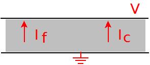
Figure 2: Capacitance with a leak current $I_{f}$. In Fourier frequency space, the voltage difference $V$ and the current density $j$ obey $\vec{j}=[\sigma_{e}+i\omega\varepsilon]~{}\frac{V}{d}$ when the electric parameters do not depend on frequency. $d$ is the distance between the arms of the capacitor. The density of the leak current is given by $j_{f}=\sigma_{e}V$ that of the capacitive current is $j_{c}=i\omega\varepsilon V$ . We also have $I_{f}=j_{f}A$ and $I_{c}=j_{c}A$ where $A$ is the area of the arms.

If we now assume the following equalities:

$$\bf{\gamma}(\vec{r},\infty)=\bf{\sigma}(\vec{r},\infty)+i\omega\bf{\varepsilon}(\vec{r},\infty)~{}~{}et~{}~{}\bar{\Delta}\bf{\gamma}=\bf{\gamma}(\vec{r},\omega)-\bf{\gamma}_{\infty}$$ (28)

Applying Equations (16) and (25), we can write:

$$\bar{\Delta}\bf{\gamma}=\bar{\Delta}\bf{\gamma}^{\prime}+i\bar{\Delta}\gamma^{\prime\prime}=[\bar{\Delta}\bf{\sigma}_{e}^{\prime}-\mathcal{H}(\omega\bar{\Delta}\bf{\varepsilon}^{\prime})]+i~{}[\omega\bar{\Delta}\bf{\varepsilon}^{\prime}+\mathcal{H}(\bar{\Delta}\bf{\sigma}_{e}^{\prime})]$$ (29)

It follows that

$$\left\{\begin{array}[]{ccccc}\bar{\Delta}\bf{\gamma}^{\prime\prime}=\mathcal{H}~{}(\bar{\Delta}\bf{\gamma}^{\prime})&(a)\\ \\ \bar{\Delta}\bf{\gamma}^{\prime}=-\mathcal{H}~{}(\bar{\Delta}\bf{\gamma}^{\prime\prime})&(b)\end{array}\right.$$ (30)

because the Hilbert transform obeys $-\mathcal{H}^{2}~{}(F)=F$. We can also write

$$\bar{\Delta}\bf{\gamma}=\bf{\bar{\Delta}\gamma}^{\prime}+i~{}\mathcal{H}~{}(\bf{\bar{\Delta}\gamma^{\prime}})~{}~{}$$ (31)

such that the phase $\phi$ obeys

$$tan(\phi)=\frac{\mathcal{H}(\bf{\bar{\Delta}\gamma^{\prime}})}{\bf{\bar{\Delta}\gamma}^{\prime}}$$ (32)

For a sufficiently large base volume, we can always assume that the conductivity and permittivity do not depend on position. In this particular case, we can write

$$\left\{\begin{array}[]{cccccc}I^{g}&=&\iint\limits_{\mathcal{S}_{eq}}\vec{j}\cdot\hat{n}~{}dS&=&<\parallel\vec{j}\parallel>_{\mathcal{S}}S&(a)\\ \\ \Delta V&=&\int_{a}^{b}\nabla V\cdot\hat{n}~{}ds&=&\frac{<\parallel\vec{j}\parallel>_{l}}{\gamma(\omega)}l&(b)\end{array}\right.$$ (33)

where the current $I^{g}$ is conserved. $<\parallel\vec{j}\parallel>_{\mathcal{S}}$ is the mean current density over an equipotential surface and $<\parallel\vec{j}\parallel>_{l}$ is the mean current density along a current line between two equipotential surfaces. These two means are different in general, but if we take the curve that goes through the mean current density $<\parallel\vec{j}\parallel>_{\mathcal{S}}$ over each equipotential surface, then we can say that this curve is a current line. Consequently, there exists an equipotential surface and a current line such that $<\parallel\vec{j}\parallel>_{\mathcal{S}}=<\parallel\vec{j}\parallel>_{l}$. It follows that, if $A_{\mathcal{C}}$ is the area of this surface, and $l_{\mathcal{C}}$ is the distance between two isopotential surfaces, then we can write

$$\frac{I^{g}}{\Delta V}=\gamma(\omega)~{}\frac{A_{\mathcal{C}}}{l_{\mathcal{C}}}$$ (34)

This form is identical to that of a plane capacitor which possesses a leak current, because the real part is non-zero, or a conductance with a non-negligible capacitive effect, because the imaginary part is also non-zero.

If we define the apparent conductivity as $\sigma_{\mathcal{A}}$ as the real part of $\bf{\gamma}$

$$\sigma_{\mathcal{A}}=\gamma^{\prime}=\sigma_{e}^{\prime}-\omega\varepsilon^{\prime\prime}$$ (35)

and the apparent permittivity $\varepsilon_{\mathcal{A}}$ times the angular frequency $\omega$ as the imaginary part of $\bf{\gamma}$

$$\omega\varepsilon_{\mathcal{A}}=\gamma^{\prime\prime}=\omega\varepsilon^{\prime}+\sigma_{e}^{\prime\prime}~{},$$ (36)

we can then write where these apparent parameters are real and linked by a Hilbert transform . We have $\omega\bar{\Delta}\varepsilon_{\mathcal{A}}=\mathcal{H}(\bar{\Delta}\sigma_{\mathcal{A}})$ and $\bar{\Delta}\sigma_{\mathcal{A}}=-\mathcal{H}(\omega\bar{\Delta}\varepsilon_{\mathcal{A}})$.

Thus, the knowledge of one parameter is sufficient to deduce the other. For a given frequency, it is always possible to simulate the current-voltage relation between two isopotential surfaces as a plane capacitor (see Fig. 2). The leak current of this capacitor is determined by the Hilbert transform of its admittance, or by a conductance possessing a capacitive effect determined by Hilbert transform of the admittance. Finally, $\sigma_{\mathcal{A}}$ and $\varepsilon_{\mathcal{A}}$ are an even function (see Eqs. 35) and 36) relative to $\omega$.

It is important to note that, for the apparent parameters, as defined in Eqs. 35 and 36, we have the following properties. First, the apparent conductivity is equal to the electric conductivity when $\omega=0$, or when the imaginary part of the electric permittivity is zero. Second, the apparent permittivity becomes infinitely large for $\omega=0$ when the imaginary part of the electric conductivity is different from zero. Third, if the imaginary parts of both electric conductivity and permittivity are zero, then the apparent parameters are identical to electric parameters. Finally, if the physical effects associated to the electric permittivity (density of induced charges) are negligible compared to that of electric conductivity, then the apparent conductivity is approximately given by the real part of electric conductivity, and the apparent permittivity is approximately to the imaginary part of electric conductivity divided by $\omega$.

3 Applications

In this section, we consider models of different known media to illustrate the consequences of the relations outlined in the theoretical part. All models considered are built within the quasistatic approximation of the linear electromagnetic theory of Maxwell-Heaviside. In other words, we do not consider physical phenomena associated to electromagnetic induction ($\nabla\times\vec{\bf{E}}=0$). In such conditions, we can apply the Kramers-Kronig relations (or Hilbert transform) over the approximated electric parameters .

3.1 Constraints on the conductivity given by the Kramers-Kronig relations

3.1.1 First example

As a first example, we consider an isotropic medium where the base volume of the mean-field does not depend on position. We suppose that the medium is such that $\sigma_{e}$ depends on frequency with a null imaginary part, and that $\lim\limits_{\omega\rightarrow\infty}\sigma_{e}=k$ is real and frequency independent. This model would correspond to a heterogeneous and isotropic medium where the conductivity depends on frequency $\nu$ according to a law $\sigma_{e}(\omega=2\pi\nu)=\sigma_{e}^{\prime}(\omega)+i\sigma_{e}^{\prime\prime}(\omega)=\sigma_{e}^{\prime}(\omega)$.

In this case, according to Eq. (26b), we must have

$$\sigma_{e}^{\prime}(\omega)=\sigma(\infty)=k$$ (37)

because $\bar{\Delta}\sigma_{e}^{\prime}=0$ when $\bar{\Delta}\sigma_{e}^{\prime\prime}=0$. Therefore, according to Kramers-Kronig relations, $\sigma_{e}^{\prime}$ would not depend on frequency, which is contradictory with the initial hypothesis.

Thus, a model of this kind is not acceptable, because we have a contradiction with the causality principle because the Kramers-Kronig relations are a direct consequence of this principle in a linear system.

For example, it is impossible to have a conductivity law of the form $\sigma_{e}=\omega^{x}e^{-\omega/c}+k$ where x is arbitrary. One must add an imaginary part, which implies that the phase is non-zero. Thus, a model with a frequency-dependent conductivity but a null phase is physically impossible in a model where conductivity becomes resistive or if the phase becomes zero at high frequencies . Note that, in general, the electric conductivity is not necessarily real for large frequencies. It was shown before that the linear approximation of a physical system with ionic diffusion gives an electric conductance of the form $\sqrt{\omega}(a+ib)$ [10]. Thus, the asymptotic behavior of the electric conductivity at high frequencies is very different from the electric permittivity, because the latter tends to the permittivity of vacuum, which is real.

For example, let us consider the model examined by Miceli et al. [5] of a medium in which the electric conductivity is frequency-dependent, but the permittivity is constant. According to above, such a medium is physically impossible, because it would violate the principle of causality. It is important to note that the standard model of a resistive extracellular medium, the capacitive effects are neglected.

The Miceli model is asymptotically resistive at high frequencies ($\lim\limits_{\omega\rightarrow\infty}\sigma_{e}=k$), and thus, we can conclude that, if the conductivity depends on frequency, one must necessarily have both real and imaginary parts different from zero for the model to be physically plausible.

3.1.2 Second example

In this section, we suppose that the apparent macroscopic permittivity $\varepsilon_{\mathcal{A}}$ between two equipotential surfaces is given by

$$\begin{array}[]{cccccc}\varepsilon_{\mathcal{A}}&=&\varepsilon_{o}+\frac{\kappa}{|\omega|^{2+x}}\end{array}$$ (38)

where $x,\kappa\in\mathbb{R}$ and $x\geq-1$, and $\kappa\geq 0$ and frequency-independent. Note that this model respects the parity of $\varepsilon_{\mathcal{A}}$ (see Eq. 36) because we have $\varepsilon_{\mathcal{A}}(+\omega)=\varepsilon_{\mathcal{A}}(-\omega)$. This simple model corresponds to a physical situation where the apparent permittivity diminishes for increasing frequency, and approaches that of vacuum for very high frequencies. This situation is often encountered in heterogeneous media such as biological tissues (see for example, the experimental measurements of Gabriel et al. [2]).

Note that if the apparent permittivity $\varepsilon_{\mathcal{A}}$ tends to that of vacuum, then the electric conductivity $\sigma_{e}$ must necessarily have a zero phase when frequency tends to infinity (see Eq. 36) because the real part of the electric permittivity $\varepsilon$ tends to that of vacuum.

By applying Eq. (30b) and assuming that $y=\frac{\omega_{a}}{w}$, we obtain:

$$\bar{\Delta}\sigma_{\mathcal{A}}(\omega)=-\mathcal{H}~{}(\bar{\Delta}\omega\varepsilon_{\mathcal{A}})=-\frac{2~{}\kappa}{\pi\omega^{1+x}}\fint_{~{}0}^{+\infty}\frac{1}{(y^{2}-1)y^{x}}dy=-\frac{\kappa_{1}}{\omega^{1+x}}$$ (39)

where we have

$$\kappa_{1}=\frac{2~{}\kappa}{\pi}\fint_{~{}0}^{+\infty}\frac{1}{(y^{2}-1)y^{x}}dy$$ (40)

Consequently, the phase of the admittance variation is such that

$$tan{(\phi)}=\frac{\bar{\Delta}(\omega\varepsilon_{\mathcal{A}})}{\bar{\Delta}(\sigma_{\mathcal{A}})}=-\frac{\kappa}{\kappa_{1}}$$ (41)

when $\omega>0$ and $+\frac{\kappa}{\kappa_{1}}$ for $\omega<0$. Note that $\kappa_{1}$ depends on the value of the exponent $x$. Also note that the phase of the admittance variation $\Delta\gamma$ does not depend on frequency in this type of model.

We now calculate the phase for different values of the exponent $x$. The principal part of the integral in expression (40) is explicitly given by the following expression:

$$\kappa_{1}=\lim\limits_{\delta\rightarrow 0}~{}{\Big{[}}\int_{\delta}^{1-\delta}\frac{1}{(y^{2}-1)y^{x}}dy+\int_{1+\delta}^{1/\delta}\frac{1}{(y^{2}-1)y^{x}}dy~{}{\Big{]}}$$ (42)

where $\delta>0$.

Case x=0.

For $x=0$, Eq. (42) becomes

$$\kappa_{1}=\frac{2~{}\kappa}{\pi}~{}\lim\limits_{\delta\rightarrow 0}~{}In~{}{\Big{[}}\frac{-\delta}{2-\delta}\cdot\frac{\delta+1}{\delta-1}\cdot\frac{1-\delta}{1+\delta}\cdot\frac{2+\delta}{\delta}{\Big{]}}=0$$ (43)

It follows that the phase of the admittance variation is given by $\phi=-\frac{\pi}{2}$ for ($\omega>0$, and $\phi=\frac{\pi}{2}$ for ($\omega<0$.

Moreover, we see that the variations of apparent conductivity with frequency are such that $\bar{\Delta}\sigma_{\mathcal{A}}=0$. Thus, in this model, the apparent conductivity is equal to the real part of the electric conductivity because, for infinite frequencies, the imaginary part of electric permittivity $\varepsilon"$ tends to zero and $\varepsilon^{\prime}$ tends to that of vacuum. Thus, we have $\varepsilon_{\mathcal{A}}=\varepsilon_{o}+\frac{\kappa}{|\omega|^{2}}$ and $\sigma_{\mathcal{A}}=\sigma_{e}^{\prime}(\omega\rightarrow\infty)$. Consequently, if we assume that the medium is resistive for very high frequencies, then we see that the phase is necessarily frequency-dependent because the phase of the admittance $\gamma$ is given by $tan(\phi)=\frac{\omega\varepsilon_{0}+\frac{\kappa}{\omega}}{\sigma_{e}^{\prime}}$ for $\omega>0$.

Case $x=\pm 1/2$ .

In this case, the primitives of the integrals in expression (42) are:

$$\frac{1}{2}In~{}{\Big{[}}\frac{1-\sqrt{y}}{1+\sqrt{y}}{\Big{]}}\mp tg^{-1}\sqrt{y}$$ (44)

It follows that

$$\kappa_{1}=\frac{2~{}\kappa}{\pi}~{}\lim\limits_{\delta\rightarrow 0}~{}In~{}{\Big{[}}\frac{1-\sqrt{1-\delta}}{1+\sqrt{1+\delta}}\cdot\frac{1+\sqrt{\delta}}{1-\sqrt{\delta}}\cdot\frac{1-\sqrt{1/\delta}}{1+\sqrt{1/\delta}}\cdot\frac{1+\sqrt{1+\delta}}{1-\sqrt{1+\delta}}{\Big{]}}+t=t$$ (45)

where

$$t=\mp\frac{2~{}\kappa}{\pi}\lim\limits_{\delta\rightarrow 0}~{}[tg^{-1}\sqrt{1-\delta}-tg^{-1}\sqrt{\delta}+tg^{-1}\sqrt{1/\delta}-tg^{-1}\sqrt{1+\delta}]=\mp\kappa$$

Thus, the phase (Eq. 41) of the admittance variation is given by $\phi=\pm\frac{\pi}{4}$, because we have

$$tan{(\phi)}=\frac{\bar{\Delta}(\omega\varepsilon_{\mathcal{A}})}{\bar{\Delta}(\sigma_{\mathcal{A}})}=\pm 1$$ (46)

Consequently, the admittance variation $\bar{\Delta}\gamma_{\mathcal{A}}$ is such that $\bar{\Delta}\gamma_{\mathcal{A}}=\bar{\Delta}(\sigma_{\mathcal{A}})(1-i)$ and $\bar{\Delta}\gamma_{\mathcal{A}}=\bar{\Delta}(\sigma_{\mathcal{A}})(1+i)$ when we have, respectively, $\varepsilon_{\mathcal{A}}=\varepsilon_{o}+\frac{\kappa}{|\omega|^{3/2}}$ and $\varepsilon_{\mathcal{A}}=\varepsilon_{o}+\frac{\kappa}{|\omega|^{5/2}}$

This result is interesting for the following reason: we note that if we consider the case where the exponent equals $-3/2$ for $\bar{\Delta}\varepsilon_{\mathcal{A}}$, then we have $\bar{\Delta}\sigma_{\mathcal{A}}<0$. This corresponds to a situation where conductivity increases with frequency. On the other hand, if the exponent equals $-5/2$, then the apparent conductivity decreases with frequency. The first case seems in agreement with experimental measurements (see [2]).

It follows that, for the first case (exponent of -3/2), we can write:

$$\gamma_{\mathcal{A}}=\bar{\Delta}\gamma_{\mathcal{A}}+\gamma_{\mathcal{A}}(\omega=\infty)=\bar{\Delta}(\sigma_{\mathcal{A}})(1-i)+\gamma_{\mathcal{A}}(\omega=\infty)$$ (47)

We see that if the apparent admittance tends asymptotically to a constant $C$ (independent of frequency) for high frequencies, then we have $C\approx\bar{\Delta}(\sigma_{\mathcal{A}})$, so there will be a non-negligible phase at low frequencies. We recall that, by definition, we have $\lim\limits_{\omega\rightarrow\infty}\bar{\Delta}(\sigma_{\mathcal{A}})=0$ (see Eq. 28).

We also see that if the product $\omega\varepsilon$ is negligible compared to electric conductivity, and if the latter tends to a Warburg impedance for high frequencies (as in ref. [21]), then, according to the definition of apparent parameters (Eqs. 35 and 36), we can write:

$$\gamma_{\mathcal{A}}=\gamma_{e}=(\bar{\Delta}(\sigma_{\mathcal{A}})+k)\sqrt{\omega}~{}(1\pm i)$$ (48)

where $\gamma_{e}$ is the electric admittance.

Case x arbitrary and greater than -1.

For an arbitrary value of $x$, we can write

$$tan{(\phi)}=\frac{\bar{\Delta}(\omega\varepsilon_{\mathcal{A}})}{\bar{\Delta}(\sigma_{\mathcal{A}})}=cst~{}$$ (49)

such that we can write

$$\gamma_{\mathcal{A}}=\bar{\Delta}\gamma_{\mathcal{A}}+\gamma_{\mathcal{A}}(\omega=\infty)=\bar{\Delta}(\sigma_{\mathcal{A}})(1+tan{(\phi)}~{}i)+\gamma_{\mathcal{A}}(\omega=\infty)$$ (50)

where the phase $\gamma_{\mathcal{A}}$ is frequency dependent because $\bar{\Delta}(\sigma_{\mathcal{A}})$ depends on frequency.

Finally, we see that if the electric permittivity varies according to the following law:

$$\begin{array}[]{cccccc}\varepsilon_{\mathcal{A}}&=&\varepsilon_{o}+\sum\limits_{j=1}^{N}\frac{\kappa_{j}}{|\omega|^{2+x_{j}}}\end{array}$$ (51)

where $x_{j}>-1$, then we can calculate the phase of the apparent electric admittance, by fitting the expression (51) to the measured electric permittivity. Note that in these examples, this phase is non-negligible when the electric or apparent parameters (admittance, conductivity, permittivity) are frequency dependent.

4 Discussion

In this paper, we have re-examined electromagnetism theory in heterogeneous media, in particular focusing on the Kramers-Kronig relations, following the Landau & Lifshitz formalism [11]. Our main finding is that, similar to the well-known Kramers-Kronig relations linking the real and imaginary parts of the electric permittivity [11], one can also derive similar relations for electric conductivity. Thus, in heterogeneous media, the two electric parameters obey symmetric dependencies in Fourier frequency space. This finding is general, and also applies to a homogeneous medium (which is a particular case of heterogeneous media). We discuss below the significance of these results.

As a first example, we considered the model of a medium where electric conductivity was assumed to be frequency-dependent, but with a constant permittivity [5]. We showed that, according to Kramers-Kronig relations, this model is physically impossible, as it would violate the principle of causality. This models is also asymptotically resistive at high frequencies ($\lim\limits_{\omega\rightarrow\infty}\sigma_{e}=k$), and thus, we can conclude that, if the conductivity depends on frequency, one must necessarily have both real and imaginary parts different from zero for such a model to be physically plausible. It is important to note that the NEURON simulator [7] used for such simulations cannot deal with complex electric parameters (non-negligible phase), so cannot be used to simulate physically-plausible non-resistive situations.

In a second example, we considered experimental measurements suggesting that the extracellular medium around neurons is non-resistive [4, 6]. We showed here that these measurements are consistent with Kramers-Kronig relations, and the principle of causality. However, other measurements suggesting resistive media [3, 5], are also consistent with Kramers-Kronig relations. All these experimental measurements are thus physically plausible and self-consistent. On the modeling point of view, the models of non-resistive media [4, 9, 10, 19], as well as those of resistive media [5], are all consistent with Kramers-Kronig relations as well. One notable exception is the non-resisistive models examined in [5], which are non-plausible, as discussed above. Note that ionic diffusion was proposed as a mechanism to explain the non-resistive measurements [4, 6, 9], and according to this mechanism, the phase of the apparent admittance should tend to $\pi/4$ at high frequencies (Warburg impedance). This value seems in agreement with phase measurements in cerebral cortex [4, 8] and retina [21], and is also consistent with Kramers-Kronig relations.

A further interesting property, developed Section 2.4, is that the apparent permittivity is far from negligible at very low frequencies when the imaginary part of the electric conductivity is non zero, even if it is very small. This property must be related to the difficulty of measuring the impedance (or admittance) at low frequencies [2, 3, 4, 8]. This difficulty could be the sign that the apparent permittivity increases rapidly at low frequencies (lower than $\sim$10 Hz). This phenomenon should not appear in a resistive medium.

We conclude that, given the constraints imposed by Kramers-Kronig relations, the previous experimental measurements seems internally consistent for frequencies larger than 10 Hz, either for resistive [3, 5] or non-resistive media [2, 4]. Further experiments are needed to distinguish between these two alternatives, as reviewed in detail previously [6].

References

- [1]
- [2] Gabriel, S., Lau, R.W. and Gabriel, C., Phys. Med. Biol. 41, 2251 (1996).
- [3] Logothetis NK, Kayser C, Oeltermann A., Neuron 55, 809 (2007).
- [4] Gomes JM, Bédard C, Valtcheva S, Nelson M, Khokhlova V, Pouget P, Venance L, Bal T and Destexhe, A. Biophys. J. 110, 234 (2016)
- [5] Miceli S, Ness TV, Einevoll, GT and Schubert D., eNeuro 4, e0291 (2017)
- [6] Bédard C., Gomes, J-M., Bal, T. and Destexhe A., J. Integrative Neurosci. 16, 3 (2017).
- [7] Hines M.L. and Carnevale N.T. Neural Computation 9, 1179 (1997).
- [8] Bédard C., Destexhe A., Biophys J. 113 7, 1639 (2017)
- [9] Bédard, C. and Destexhe, A. Biophys. J. 96, 2589 (2009)
- [10] Bédard, C. and Destexhe, A., Physical Review E 84: 041909 (2011)
- [11] Landau, L.D. and E.M. Lifshitz Electrodynamics of Continuous Media. Pergamon Press, Moscow, Russia, (1981).
- [12] Kronig, R.D.L., J. Opt. Soc. Am.. 12, 547 (1926)
- [13] Foster, KR. and HP. Schwan, Crit. Reviews Biomed. Engineering. 17: 25 (1989).
- [14] Appel, W. Mathematics for Physics and Physisics, Princeton University Press (2007)
- [15] M. Schönleber, D. Klotz and E. Ivers-Tiffée, Electrochimica Acta 131, pp. 20 (2014).
- [16] Le Bellac M. and Levy-Leblond J.-M., Nuevo Cimento 14B, N.2 (aprile), 1973.
- [17] Rousseaux, G. Europhysics Letters, European Physical Society/EDP Sciences/Società Italiana di Fisica/IOP Publishing, 71 (1), p. 15 (2005).
- [18] Bedard, C. and Destexhe, A., Modeling local field potentials and their interaction with the extracellular medium. In: Handbook of Neural Activity Measurement, Edited by Brette R. and Destexhe A., Cambridge University Press, Cambridge, UK, pp. 136 (2012).
- [19] Bédard, C. and Destexhe, A., Physical Review E, 88, 022709 (2013)
- [20] Bédard, C. and Destexhe A., Physical Review E 90, 042723 (2014)
- [21] Pham P, Roux S, Matonti F, Dupont F, Agache V and Chavane F., J. Neural Eng. 10, 046002 (2013)