Phase Diagrams of Antiferromagnetic Spin-1 Bosons on Square Optical Lattice with the Quadratic Zeeman Effect

Abstract

We study the quadratic Zeeman effect (QZE) in a system of antiferromagnetic spin-1 bosons on a square lattice and derive the ground-state phase diagrams by means of quantum Monte Carlo simulations and mean field treatment. The QZE imbalances the populations of the magnetic sublevels $\sigma=\pm 1$ and $\sigma=0$, and therefore affects the magnetic and mobility properties of the phases. Both methods show that the tip of the even Mott lobes, stabilized by singlet state, is destroyed when turning on the QZE, thus leaving the space to the superfluid phase. Contrariwise, the tips of odd Mott lobes remain unaffected. Therefore, the Mott-superfluid transition with even filling strongly depends on the strength of the QZE, and we show that the QZE can act as a control parameter for this transition at fixed hopping. Using quantum Monte Carlo simulations, we elucidate the nature of the phase transitions and examine in detail the nematic order: the first-order Mott-superfluid transition with even filling observed in the absence of QZE becomes second order for weak QZE, in contradistinction to our mean field results which predict a first-order transition in a larger range of QZE. Furthermore, a spin nematic order with director along the $z$ axis is found in the odd Mott lobes and in the superfluid phase for energetically favored $\sigma=\pm 1$ states. In the superfluid phase with even filling, the $xy$ components of the nematic director remain finite only for moderate QZE.

I Introduction

The use of ultracold bosonic systems as simulators for the Bose-Hubbard model, proposed in 1998,Jaksch_1998 quickly led to an experimental realization of the Mott-superfluid transition in 2002.Greiner02 For the first time, ultracold gases experiments allowed the simulation of well-known condensed-matter systemsFisher_1989 and strongly correlated states – e.g., Mott insulating state – thus connecting two so far distinct fields: atomic physics and condensed-matter physics. Since then, ultracold atoms in optical lattices are referred to as quantum simulators, i.e., highly tunable systems suitable for the exploration of quantum statistical lattice models,bloch08 such as the Bose Greiner02 and Fermi Chin_2006 ; Schneider08 ; Jordens08 Hubbard models.

Since the seminal work of Jaksch et al. in 1998,Jaksch_1998 the motivation for considering many species of atoms, or internal degree of freedom, has emerged from the promising perspectives of observing coexisting phases, quantum magnetism, and spin dynamics. Dalibard_Gerbier_2011 ; Gerbier_2006_qnegatif ; Stamper_Kurn_2013 ; Zhao_2015 ; Lewenstein_Sanpera_1998 ; Kawaguchi_Ueda_2012 ; Krutitsky_2016 ; Kuklov_Svistunov_2003 ; Chang_2005 ; Lamacraft_2010 Indeed, mutlicomponent Bose-Einstein condensates, also called spinor condensates, are ideal systems for engineering quantum phase transitions,Liu_2016 entanglement, metrology,Esteve_2008 thermometry,Weld_Lingua and have possible applications in astrophysicsAlpar_1984_Lattimer_2004 and in quantum chromodynamics.Son_2001_2002_Tylutki_2016 The spin degrees of freedom allow the study of multi band condensed matter Hamiltonians and the interplay between magnetism and superfluidity.Vengalattore08 ; Vengalattore10 Contrary to the standard Bose-Hubbard model with U(1) symmetry, spinor condensates in optical lattice are described by the extended Bose-Hubbard model where spin-spin interactions introduce an additional symmetry.Ho_1998 ; ohmi98 The spontaneous breaking of this additional symmetry leads to the establishment of quantum magnetism in the Mott insulating and superfluid phases, and to multiple transitions. Imambekov_2004 ; snoek04 ; Capogrosso_Sansone_2010 ; Deforges_2013 ; deforges2014 ; deforges2015 ; deforges2016 The on-site spin-spin interaction can be tuned by using Feshbach resonance Theis and the nature of the spin-spin interaction can be either ferromagnetic (e.g., ${}^{87}{\rm Rb}$) or antiferromagnetic (e.g., ${}^{23}{\rm Na}$) depending on the relative magnitudes of the scattering lengths in the singlet and quintuplet channels.Stamperbook

The ground-state phase diagram has been intensively investigated using many methods: static and dynamical mean-field theory,pai08 ; tsuchiya05 ; kruti04 ; Li_2016 variational Monte Carlo,toga analytical,Imambekov_2004 ; demler02 ; Katsura strong coupling expansion, Kimura13 density matrix renormalization group, Rizzi05_dmrg ; Bergkvist06_dmrg and quantum Monte Carlo simulations.apaja06 ; batrouni2009 ; Deforges_2013 Similar to the standard Bose-Hubbard model, the system adopts Mott-insulating (MI) phases, when the filling is commensurate with the lattice size and for large enough repulsion between particles, and a superfluid phase (SF) otherwise. The richness of these systems comes from the magnetic behavior of these phases. The two-dimensional case with antiferromagnetic spin-spin interactions is particularly interesting: a singlet state, with vanishing local magnetic moment, is observed in the MI phases with even filling and a nematic state, i.e. a non trivial state breaking spin-rotation symmetry without magnetic order, is observed otherwise. These magnetic properties are well described by the bilinear-biquadratic Heisenberg model in the strong-coupling limit at integer filling.Imambekov_2004 ; Kawashima02 ; Tsuchiya04 ; DeChiara_2011 ; Zhou_2004 In the weak-coupling limit, the magnetic properties of the superfluidity can be investigated within the single mode approximation, where spin and spatial degree of freedom are decoupled.Jacob_2012 ; Zibold_2016 ; Black_2007 ; Liu_PRL_2009 Moreover, the phase transitions are affected by the spin-spin interactions: the MI-SF transition is first order for even densities (second order otherwise),Liu_2016 ; kruti05 ; pai08 ; tsuchiya05 ; toga ; Deforges_2013 and a singlet-nematic transition occurs inside the MI phases with even densities for small spin-spin interactions.Imambekov_2004 ; snoek04 ; Deforges_2013 ; deforges2014

The addition of an external magnetic field completely changes the picture: the square of the external magnetic field $B^{2}$, coupled with the square of the local magnetic moment $S_{z}^{2}$, lifts the degeneracy between the magnetic sublevels $\sigma=\pm 1$ and $\sigma=0$, and thus constraints the populations of these sublevels. This effect, called the quadratic Zeeman effect in the literature, does not lift the degeneracy between the states $\sigma=+1$ and $\sigma=-1$, contrary to the Zeeman effect. Therefore, the square of the magnetic field in the QZE is equivalent to the impurities in the Blume-Capel model in condensed-matter physics.Blume_Capel This QZE, which has been mostly studied in dilute gas within the single mode approximation, acts as a control parameter for the magnetic structure of the superfluidity.Jacob_2012 ; Zibold_2016 ; Jiang_2014 ; Zhao_2015 Our study completes the picture for strong interacting particles in optical lattices. As shown below, the QZE not only affects the spin degrees of freedom, but also impacts the mobility of the particles and, therefore, the phase coherence. Furthermore, it was experimentally observed that the nature of the MI-SF transition with even densities is strongly affected by the QZE.Liu_2016

The purpose of this paper is to extend our preliminary studyDeforges_2013 by considering the QZE in the antiferromagnetic spin-1 system at zero temperature. We derive the phase diagrams and investigate the magnetic structure, thanks to the correlations functions accessible with the QMC method. The paper is organized as follows: In Sec. II, we introduce the model and the methods used to study it. The mean-field and QMC phase diagrams are discussed in Sec. III and Sec. IV, respectively. The results obtained by both methods are compared in Sec. IV. In Sec. V, we summarize these results and give some final remarks.

II Hamiltonian and Methods

II.1 Spin-1 Bose-Hubbard model with the quadratic Zeeman energy

We consider a system of bosonic atoms in the hyperfine state $F=1$ characterized by the magnetic quantum number $F_{z}=\{\pm 1,0\}$. When these atoms are loaded in an optical lattice, the system is governed by the extended Bose-Hubbard Hamiltonian:Mahmud_2013 ; Imambekov_2004 ; Ho_1998

$$\mathcal{\hat{H}} = -t\sum_{\sigma,\langle\bf r,\bf r^{\prime}\rangle}\left(a^{\dagger}_{\sigma\bf r}a^{\phantom{\dagger}}_{\sigma\bf r^{\prime}}+{\rm h.c.}\right)+\frac{U_{0}}{2}\sum_{\bf r}{\hat{n}}_{\bf r}\left({\hat{n}}_{\bf r}-1\right)$$ (1)

$$+\frac{U_{2}}{2}\sum_{\bf r}\left({\bf{\hat{S}}}_{\bf r}^{2}-2{\hat{n}}_{\bf r}\right)-q\sum_{\bf r}{\hat{n}}_{0\bf r},$$

where operator $a^{\phantom{\dagger}}_{\sigma{\bf r}}$ ($a^{\dagger}_{\sigma{\bf r}}$) annihilates (creates) a boson in the Zeeman state $\sigma=\{\pm 1,0\}$ (or $\sigma=\{\downarrow,0,\uparrow\}$) on site ${\bf r}$ of a periodic square lattice of size $L\times L$.

The first term in the Hamiltonian is the kinetic term which allows particles to hop between neighboring sites $\langle{\bf r,r^{\prime}}\rangle$ with strength $t$. The number operator $\hat{n}_{{\bf r}}\equiv\sum_{\sigma}{\hat{n}}_{\sigma\bf r}=\sum_{\sigma}a^{\dagger}_{\sigma{\bf r}}a^{\phantom{\dagger}}_{\sigma{\bf r}}$ counts the total number of bosons on site $\bf r$. $N_{\sigma}\equiv\sum_{\bf r}\langle{\hat{n}}_{\sigma{\bf r}}\rangle$ will denote the total number of $\sigma$ bosons, $\rho_{\sigma}\equiv N_{\sigma}/L^{2}$ the corresponding density, and $\rho\equiv\sum_{\sigma}\rho_{\sigma}$ the total density. The operator ${\bf{\hat{S}}}_{\bf r}=({\hat{S}}_{x,{\bf r}},{\hat{S}}_{y,{\bf r}},{\hat{S}}_{z,{\bf r}})$ is the spin operator where ${\hat{S}}_{\alpha,{\bf r}}=\sum_{\sigma,\sigma^{\prime}}a^{\dagger}_{\sigma\bf r}J_{\alpha,\sigma\sigma^{\prime}}a_{\sigma^{\prime}\bf r}$, $\alpha=\{x,y,z\}$ and the $J_{\alpha,\sigma\sigma^{\prime}}$ are standard spin-1 matrices; hence

$$\left\{\begin{array}[]{lll}\vspace*{0.2 cm}{\hat{S}}_{x,{\bf r}}&=&\frac{1}{\sqrt{2}}\left(({a}^{\dagger}_{\downarrow{\bf r}}+{a}^{\dagger}_{\uparrow{\bf r}}){a}_{0{\bf r}}^{\phantom{\dagger}}+{a}^{\dagger}_{0{\bf r}}({a}_{\downarrow{\bf r}}^{\phantom{\dagger}}+{a}_{\uparrow{\bf r}}^{\phantom{\dagger}})\right)~{},\\ \vspace*{0.2 cm}{\hat{S}}_{y,{\bf r}}&=&\frac{\textrm{1}}{\sqrt{2}}\left(({a}^{\dagger}_{\downarrow{\bf r}}-{a}^{\dagger}_{\uparrow{\bf r}}){a}_{0{\bf r}}^{\phantom{\dagger}}-{a}^{\dagger}_{0{\bf r}}({a}_{\downarrow{\bf r}}^{\phantom{\dagger}}-{a}_{\uparrow{\bf r}}^{\phantom{\dagger}})\right)~{},\\ {\hat{S}}_{z,{\bf r}}&=&{\hat{n}}_{\uparrow{\bf r}}-{\hat{n}}_{\downarrow{\bf r}}~{}.\end{array}\right.$$ (2)

The parameters $U_{0}$ and $U_{2}$ are the on-site spin-independent and spin-dependent interaction terms. The nature of the bosons determines the sign of $U_{2}$ and consequently the nature of the on-site spin-spin interaction, whereas the spin-independent part is always repulsive, $U_{0}>0$. The $U_{2}<0$ case (e.g., ${}^{87}{\rm Rb}$Kempen_2002 ) maximizes the local magnetic moment

$$S^{2}(0)\equiv\frac{1}{L^{2}}\sum_{\bf r}\langle{\hat{\bf S}}_{{\bf r}}^{2}\rangle.$$ (3)

Therefore, this is referred to as the “ferromagnetic” case, whereas the $U_{2}>0$ case (e.g. ${}^{23}{\rm Na}$Burke_1998 ; Imambekov_2004 ), which favors minimum local magnetic moment, is referred to as “antiferromagnetic”. In this article, the hopping parameter sets the energy scale $t=1$ and we focus on ${}^{23}{\rm Na}$ atoms, i.e., $U_{2}=0.036U_{0}$.Burke_1998 ; Imambekov_2004

The fourth term in Eq. (1) corresponds to the Zeeman energy shift between the sublevels $\sigma=\pm 1$ and $\sigma=0$ with amplitude $q$. The parameter $q$ arises either from an applied magnetic field $B$, which leads to the quadratic Zeeman energy with $q\sim B^{2}$, or from a microwave field, which in this case leads to a positive or negative $q$ value.Jiang_2014 ; Gerbier_2006_qnegatif

In the absence of Zeeman shift, i.e., $q=0$, the Hamiltonian $\mathcal{\hat{H}}$ Eq. (1) has the symmetry U(1)$\times$SU(2), associated with the total mass conservation [U(1) symmetry], times the SU(2) symmetry of the spin rotation invariance on the Bloch sphere. For $q\neq 0$, the SU(2) symmetry is reduced to U(1), leading to a model with global symmetry U(1)$\times$U(1).

Once developed, the ${\bf{\hat{S}}}^{2}_{\bf r}$ operator exhibits contact interaction terms and conversion terms between the Zeeman states, i.e., $a^{\dagger}_{0\bf r}a^{\dagger}_{0\bf r}a_{\downarrow\bf r}a_{\uparrow\bf r}+{\rm h.c.}$, which destroys a pair of particles respectively in the Zeeman states $\uparrow$ and $\downarrow$ and creates two bosons in the state $\sigma=0$, and vice-versa. Therefore, only the total number of atoms $N_{\rm tot}=\sum_{\bf r,\sigma}\langle{\hat{n}}_{\sigma{\bf r}}\rangle$, associated to the U(1) symmetry, is conserved.

II.2 Mean-Field Approximation and quantum Monte Carlo Simulations

We use a combined approach based on mean-field theory, supplemented with numerically exact quantum Monte Carlo (QMC) simulations.

Although the mean field approximation does not give quantitatively accurate values for the phase boundaries, it is a practical method which allows for the rapid reconstruction of phase diagrams.pai08 ; Imambekov_2004 ; Deforges_2011 We use a mean-field formulation based on a decoupling approximation which decouples the hopping term to obtain an effective one-site problem. Introducing the superfluid order parameter $\psi_{\sigma}\equiv\langle a^{\dagger}_{\sigma\bf r}\rangle=\langle a_{\sigma\bf r}\rangle$, we replace the creation and destruction operators on site $\bf r$ by their mean values $\psi_{\sigma}$. Since we are interested in equilibrium states of spatially uniform superfluids, the order parameters can be chosen to be real. Using this ansatz, the kinetic-energy terms, which are nondiagonal in boson creation and destruction operators, are decoupled as

$$a^{\dagger}_{\sigma\bf r}a^{\phantom{\dagger}}_{\sigma\bf r^{\prime}}\simeq(a^{\dagger}_{\sigma\bf r}+a^{\phantom{\dagger}}_{\sigma\bf r^{\prime}})\psi_{\sigma}-\psi_{\sigma}^{2}~{}.$$

The Hamiltonian Eq. (1) is rewritten as a sum over local terms $\mathcal{\hat{H}}=\sum_{\bf r}\mathcal{\hat{H}}^{MF}_{\bf r}$, where

$$\mathcal{\hat{H}}^{MF}_{\bf r} = -zt\sum_{\sigma}\left[(a^{\dagger}_{\sigma{\bf r}}+a^{\phantom{\dagger}}_{\sigma{\bf r}})\psi_{\sigma}-\psi_{\sigma}^{2}\right]+\frac{U_{0}}{2}{\hat{n}}_{\bf r}\left({\hat{n}}_{\bf r}-1\right)$$ (4)

$$+\frac{U_{2}}{2}\left({\bf{\hat{S}}}_{\bf r}^{2}-2{\hat{n}}_{\bf r}\right)-q{\hat{n}}_{0\bf r},$$

where $z=4$ is the number of nearest neighbors in a square lattice. The mean-field Hamiltonian Eq. (4) can be easily diagonalized numerically in a finite occupation-number basis $\{|n_{-},n_{0},n_{+}\rangle\}$, with the truncation $n_{max}=10$, and the lowest eigenenergy is minimized with respect to $\psi_{\sigma}$. This gives the order parameters of the ground state and its eigenvector $|\Psi_{GS}^{MF}\rangle$. At zero temperature, the system is in a Bose-Einstein condensed phase if at least one of the order parameters is nonzero and is, otherwise, in an insulating phase. The condensate fractions and densities are respectively defined by

$$C^{MF}_{\sigma}\equiv|\psi_{\sigma}|^{2}~{},$$ (5)

$$\rho_{\sigma} \equiv \langle\Psi_{GS}^{MF}|a_{\sigma}^{\dagger}a_{\sigma}|\Psi_{GS}^{MF}\rangle,$$ (6)

with $C^{MF}=\sum_{\sigma}C^{MF}_{\sigma}$ the total condensate fraction.

Our QMC simulations are based on the Stochastic Green Function algorithmSGF with directed updates,directedSGF an exact quantum Monte Carlo technique that allows canonical or grand canonical simulations of the system as well as measurements of many-particle Green functions. In particular, this algorithm can simulate efficiently the conversion terms.

In this work, we used the canonical formulation where the total number of bosons $N_{\rm tot}$, is conserved whereas the individual number of bosons $N_{\sigma}$ fluctuate. The QMC algorithm also conserves the total spin along $z$, $S_{{\rm tot},z}=N_{+}-N_{-}$, which adds a constraint to the canonical one. The value of $S_{{\rm tot},z}$ in a given canonical simulation is then fixed by the choice of the initial numbers of particles. In this paper, we work in the spin sector $S_{{\rm tot},z}=0$. Due to this constraint, the magnetic physical quantities, involving $S_{\alpha,{\bf r}}$ operators, are identical for the $x$ and $y$ axes but may be different for the $z$ axis. The initial symmetry, where all three axes should behave identically, is broken in our simulations. Using this algorithm we were able to simulate the system reliably for clusters going up to $L=12$ with $N=288$ particles. A large enough inverse temperature of $\beta=2L/t$ allows one to eliminate thermal effects.

In particular, we calculate the averaged densities $\rho_{\sigma}=\sum_{\bf r}\langle{\hat{n}}_{\sigma{\bf r}}\rangle/L^{2}$ and the singlet density

$$\rho_{sg}\equiv\frac{1}{L^{2}}\langle{\hat{A}}_{sg}^{\dagger}{\hat{A}}_{sg}^{\phantom{\dagger}}\rangle~{},$$ (7)

where ${\hat{A}}_{sg}^{\dagger}=\frac{1}{\sqrt{6}}(2{\hat{a}}_{\uparrow}^{\dagger}{\hat{a}}_{\downarrow}^{\dagger}-{\hat{a}}_{0}^{\dagger}{\hat{a}}_{0}^{\dagger})$, which measures the number of pairs of bosons with a vanishing magnetic local moment. The chemical potential is defined as the discrete difference of the energy

$$\mu(N_{\rm tot})=E(N_{\rm tot}+1)-E(N_{\rm tot}),$$ (8)

which is valid in the ground state where the free energy is equal to the internal energy $E=\langle\mathcal{\hat{H}}\rangle$.

The analysis of the magnetic structure requires the calculation of the local magnetic moment $S^{2}(0)=S_{x}^{2}(0)+S_{y}^{2}(0)+S_{z}^{2}(0)$, where

$$S_{\alpha}^{2}(0)\equiv\frac{1}{L^{2}}\sum_{\bf r}\langle{{\hat{S}}}_{\alpha,{\bf r}}^{2}\rangle~{},$$ (9)

with components

$$\left\{\begin{array}[]{lll}\vspace*{0.2 cm}{\hat{S}}^{2}_{x,y,{\bf r}}&=&a_{0{\bf r}}^{\dagger}a_{0{\bf r}}^{\dagger}a_{\uparrow{\bf r}}^{\phantom{\dagger}}a_{\downarrow{\bf r}}^{\phantom{\dagger}}+a_{\downarrow{\bf r}}^{\dagger}a_{\uparrow{\bf r}}^{\dagger}a_{0{\bf r}}^{\phantom{\dagger}}a_{0{\bf r}}^{\phantom{\dagger}}\\ &+&({\hat{n}}_{0{\bf r}}+\frac{1}{2})({\hat{n}}_{\downarrow{\bf r}}+{\hat{n}}_{\uparrow{\bf r}})+{\hat{n}}_{0{\bf r}}\pm\mathcal{O}\vspace*{0.2 cm}\\ \vspace*{0.2 cm}{\hat{S}}^{2}_{z,{\bf{\bf r}}}&=&{\hat{n}}_{\uparrow{\bf r}}^{2}+{\hat{n}}_{\downarrow{\bf r}}^{2}-2{\hat{n}}_{\downarrow{\bf r}}{\hat{n}}_{\uparrow{\bf r}}\end{array}\right.$$ (10)

and $\langle\mathcal{O}\rangle=0$, $S_{x}^{2}(0)=S_{y}^{2}(0)$ using our algorithm. Since local quantities are insufficient for indicating a long range magnetic order, one needs to calculate the equal-time spin-spin correlation functions

$$S_{\alpha\alpha}({\bf R})\equiv\frac{1}{L^{2}}\sum_{\bf r}\langle{\hat{S}}_{\alpha,{\bf r}}{\hat{S}}_{\alpha,{\bf r+R}}\rangle~{},$$ (11)

and the magnetic structure factor

$$\mathcal{S}_{\alpha\alpha}({\bf k})\equiv\frac{1}{L^{2}}\sum_{\bf R}e^{i{\bf k\cdot R}}S_{\alpha\alpha}({\bf R})~{},$$ (12)

where ${\bf k}=(k_{x},k_{y})$ and $k_{x,y}$ are integer multiples of $2\pi/L$. The total global magnetization is given by $M^{2}_{\rm tot}=2M_{x}^{2}+M_{z}^{2}$ with $M_{\alpha}^{2}=\mathcal{S}_{\alpha\alpha}({\bf k=0})$. Additionally, we calculate the order parameter of the nematic phase associated to a director along the $z$ axis defined by

$$\Theta_{zz}\equiv\frac{1}{L^{4}}\sum_{\bf r,R}\langle{\hat{S}}^{2}_{z,{\bf r}}{\hat{S}}^{2}_{z,{\bf r+R}}\rangle~{}.$$ (13)

The quantity $\Theta_{zz}$ is maximized when the spins align or (randomly) antialign along the $z$ axis.

We also calculate the one body Green functions

$$G_{\sigma}({\bf R})=\frac{1}{2L^{2}}\sum_{\bf r}\langle a^{\dagger}_{\sigma{\bf r+R}}a^{\phantom{\dagger}}_{\sigma{\bf r}}+a^{\dagger}_{\sigma{\bf r}}a^{\phantom{\dagger}}_{\sigma{\bf r+R}}\rangle~{},$$ (14)

which measure the phase coherence of particles in Zeeman state $\sigma$. The density of $\sigma$ bosons with zero momentum – here after called the condensate – is defined by

$$C_{\sigma}=\frac{1}{L^{2}}\sum_{\bf R}G_{\sigma}({\bf R})~{}.$$ (15)

Finally, the superfluid density is given by Ceperley_1989

$$\rho_{s}=\frac{\langle W^{2}\rangle}{4t\beta},$$ (16)

where the total winding number $W=W_{-}+W_{0}+W_{+}$ is a topological quantity.

III Mean-Field Phase Diagrams

The minimization of the free energy of Hamiltonian Eq. (1) leads to a competition between the local magnetic moment $S^{2}(0)$ (dominant at low $|q|$) and the Zeeman term (dominant at large $|q|$). At large $|q|$, the minimization of the Zeeman term leads to an occupation of state $\sigma=0$ ($\sigma=\{\downarrow,\uparrow\}$) for positive (negative) $q$. As we will show, this competition leads to interesting effects for filling $\rho=2$ for which the local magnetic moment Eq. (9) could be fully minimized, i.e., $S^{2}(0)=0$.

III.1 Phase Diagrams

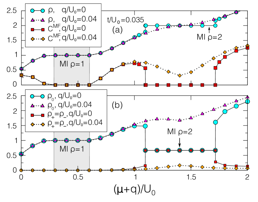
Figure 1: (Color online) Mean field data at fixed $t/U_{0}=0.035$ for $q=0$ and $q/U_{0}=0.04$. (a) The Mott phase, indicated by the $\rho=2$ plateau with $C^{MF}=0$ observed for $q=0$, disappears for $q/U_{0}=0.04$. (b) The density $\rho_{0}$ increases with $q$. The jumps in the densities and in the condensate fraction indicate first-order MI-SF transitions.

In the no-hopping limit, $t/U_{0}\to 0$, the charge gap is easily calculated: the Mott phase with one boson per site has an energy $\varepsilon(\rho=1)=0$ for $q\leq 0$ and $\varepsilon(\rho=1)=-q$ for $q>0$, whereas the Mott phase with two bosons per site has an energy

$$\varepsilon(\rho=2) = U_{0}\left(1-\frac{1}{2}\sqrt{4\left(\frac{q}{U_{0}}\right)^{2}-4q\frac{U_{2}}{U_{0}^{2}}+9\left(\frac{U_{2}}{U_{0}}\right)^{2}}\right)$$ (17)

$$- q-\frac{U_{2}}{2}~{},$$

associated to the non-degenerate wave function

$$|\Phi_{\rho=2}\rangle = \alpha|1,0,1\rangle$$ (18)

$$- \alpha\left(\frac{\sqrt{4q^{2}-4qU_{2}+9U_{2}^{2}}+2q-U_{2}}{2\sqrt{2}U_{2}}\right)|0,2,0\rangle,\ \ \ \ \ \ \$$

obtained by diagonalizing Eq. (1) in the Fock basis $|n_{-},n_{0},n_{+}\rangle=\{|1,0,1\rangle,|0,2,0\rangle\}$ with $t=0$, and $\alpha$ ensuring the normalization of the wave function.

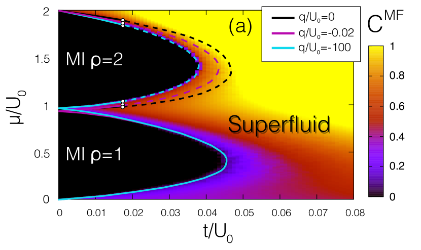
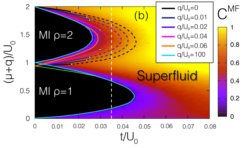
Figure 2: (Color online) Mean-field phase diagrams for $U_{2}/U_{0}=0.036$ with (a) negative $q$ and (b) positive $q$ values. Contrary to the $\rho=1$ Mott lobe, $q$ strongly affects the tip of the $\rho=2$ Mott lobe. The dashed (plain) lines indicate a first- (second-) order transition, and white dots are tricritical points. The vertical dashed line in (b) at $t/U_{0}=0.035$ corresponds to the cut shown in Fig. 1. False colors show the condensate fraction $C^{MF}$ for (a) $q/U_{0}=-100$ and (b) $q/U_{0}=100$.

For $q=0$, the on-site energy $\varepsilon(\rho=2,q=0)=U_{0}-2U_{2}$ is minimized by minimizing $S^{2}(0)=0$, that is by adopting a the singlet state given by $|\Phi_{\rho=2,q=0}\rangle=\frac{1}{\sqrt{3}}\left(\sqrt{2}|1,0,1\rangle-|0,2,0\rangle\right)$. In the limits $q\to\pm\infty$, the wave function reads $|\Phi_{\rho=2,q\to-\infty}\rangle=|1,0,1\rangle$ with energy $\varepsilon(\rho=2)=U_{0}-U_{2}$ and $|\Phi_{\rho=2,q\to+\infty}\rangle=-|0,2,0\rangle$ with energy $\varepsilon(\rho=2)=U_{0}-2q$. Therefore, for $q=0$, the base of the Mott lobes for odd filling is $\Delta\mu/U_{0}=1-2U_{2}/U_{0}$, whereas it is $\Delta\mu/U_{0}=1+2U_{2}/U_{0}$ for even filling. The even lobes grow at the expense of the odd ones, which disappear entirely for $U_{2}/U_{0}=0.5$. In the limit $q\to-\infty$, the base of the Mott lobes for odd filling is $\Delta\mu/U_{0}=1-U_{2}/U_{0}$ which disappear entirely for $U_{2}=U_{0}$, whereas it is $\Delta\mu/U_{0}=1+U_{2}/U_{0}$ for even filling. For $q\to\infty$, we recover the standard single-species Bose-Hubbard model where the base of the Mott lobes is $(\Delta\mu+q)/U_{0}=1$ for all filling ($q$ is absorbed in the chemical potential).

When turning on the hopping $t\neq 0$, the phase diagram is calculated by plotting the total density $\rho$ and the total condensate fraction $C^{MF}$ versus $\mu/U_{0}$ for many hopping $t/U_{0}$ with fixed $q/U_{0}$ value. An example of such a vertical slice in the phase diagram is plotted in Fig. 1(a) for $t/U_{0}=0.035$. We see that all compressible regions, $\kappa\equiv\partial\rho/\partial\mu\neq 0$, are superfluid with $C^{MF}\neq 0$ while the incompressible plateaus, $\kappa=0$, are not superfluid, they are the Mott insulators. Figure 1(a) also shows that increasing $q/U_{0}$ has a strong effect for $\rho>1$: the charge gap of the MI with $\rho=2$, clearly observed for $q=0$, vanishes for $q/U_{0}=0.04$. Furthermore, the population $\rho_{\pm}$ and $\rho_{0}$ are sensitive to $q$: the population of state $\sigma=0$ ($\sigma=\{\downarrow,\uparrow\}$) increases (decreases) with $q$, as expected [Fig. 1(b)]. The jump in the densities and in the condensate fraction indicate a first-order Mott-superfluid transition.pai08 ; Deforges_2013

As $t/U_{0}$ increases, the MI regions are reduced and eventually disappear. Outside the MI the system is superfluid. The evolution of the mean-field phase diagrams with respect to $q/U_{0}$ is plotted in Fig. 2.

In the $\rho=1$ Mott lobe, the local magnetic moment is fixed at $S^{2}(0)=2$ and the densities are $\rho_{-}=1$ or $\rho_{+}=1$ for $q<0$ and $\rho_{0}=1$ for $q>0$. Clearly, the tip of the $\rho=1$ Mott lobe, which ends at $t_{c}/U_{0}\simeq 0.043$, does not vary with $q$. The situation is very different for $\rho=2$, where the possible minimization of $S^{2}(0)$ competes with both the QZE and the kinetic term. For $q=0$, the tip of the $\rho=2$ Mott lobe is stabilized by the creation of the singlet state with $S^{2}(0)=0$. Since the QZE destroys the singlet state, hence $S^{2}(0)\neq 0$, we expect the superfluid region for $q\neq 0$ to grow at the expense of the $\rho=2$ Mott region. This effect is clearly observed for both negative and positive $q$ values in Fig. 2(a) and 2(b). Furthermore, the nature of the Mott-superfluid transition varies with $q$ for $\rho>1$: first- (second-) order transitions are denoted by dashed (plain) lines.

III.2 MI-SF transition versus QZE

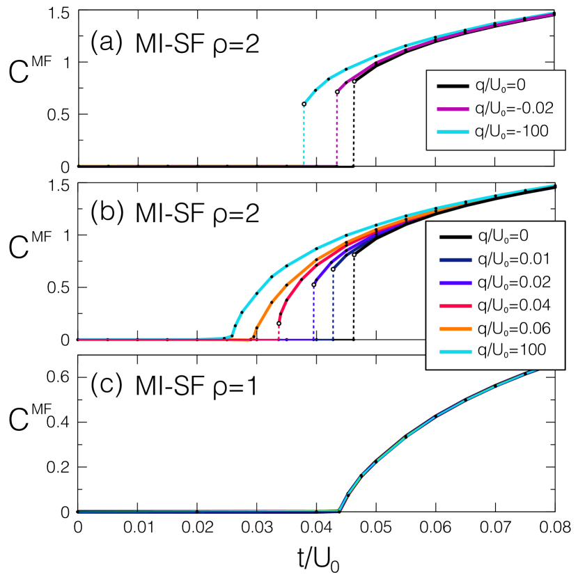
Figure 3: (Color online) Mean-field Mott-superfluid transition for (a), (b) $\rho=2$ and (c) $\rho=1$. The jump in $C^{MF}$ (vertical dashed lines) indicates a first-order transition. The transition is second order otherwise.

We first focus on the Mott-superfluid transition at fixed integer filling; see Fig. 3. As discussed before, the cases $\rho=1,2$ exhibit different behaviors, since the singlet state is destroyed by $q$ for $\rho=2$. Clearly, $q$ has no quantitative effect on the total condensate fraction $C^{MF}$ for $\rho=1$ since the local magnetic moment is fixed to $S^{2}(0)=2$ and is insensitive to $q$; see Fig. 3(c). Nevertheless, $q$ affects the distribution of the condensate populations: $C_{0}^{MF}=0$ for $q<0$, whereas $C_{\pm}^{MF}=0$ for $q>0$ (not shown). Similar to the standard single species Bose-Hubbard model using the same mean field formulation, the transition takes place at $t_{c}/U_{0}\simeq 0.043$. For $\rho=2$, the destruction of the singlet state for $q\neq 0$ leads to a shift of $t_{c}/U_{0}$ toward smaller values and the superfluid region grows at the expense of the Mott phase; see Figs. 3(a) and 3(b). We recover the single species Bose-Hubbard model with second order phase transition at $t_{c}/U_{0}\simeq 0.025$ for $q\to\infty$; see Fig. 3(b). The transition remains first-order for $q<0$, whereas the transition becomes continuous for $q/U_{0}>0.04$. Here also, $q$ affects the distribution of the condensate populations for which $C_{0}^{MF}=0$ for $q<0$, whereas $C_{\pm}^{MF}=0$ for $q>0$ (not shown).

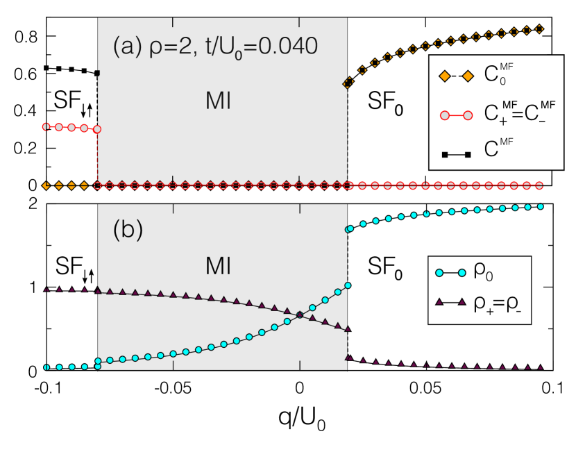
Figure 4: (Color online) Mean-field data: $q$ acts as a control parameter for the $\rho=2$ MI-SF transition at fixed hopping $t/U_{0}=0.04$. For $q\to-\infty$ the system is in the SF_↓↑ with $C_{0}^{MF}=0$ and enters in the MI phase at $q/U_{0}=-0.08$ when increasing $q$. Then, the system suddenly adopts a SF₀ phase in which $C_{\pm}^{MF}=0$ at $q/U_{0}=0.018$. Both transitions are first order.

These results are in qualitative agreement with recent observations in three-dimensional lattice.Liu_2016

The Mott-superfluid transition is also controlled by the Zeeman parameter $q$ when keeping $t/U_{0}$ fixed.Liu_2016 Figure 4 shows the successive MI-SF transitions for $t/U_{0}=0.04$ when increasing $q/U_{0}$. For $q\to-\infty$, the superfluid phase SF_↓↑ is only composed by $\sigma=\{\downarrow,\uparrow\}$ bosons [Fig. 4(a)] with balanced populations $\rho_{+}=\rho_{-}=1$ [Fig. 4(b)], whereas for $q\to\infty$, the superfluid phase SF₀ is only composed by $\sigma=0$ bosons. Interestingly enough, the system is in the $\rho=2$ MI phase for $q/U_{0}\in[-0.08,0.018]$ with non-integer densities $\rho_{\sigma}$. This effect is very similar to the one observed for molecular and atomic mixtures with species conversions for which the gap of the Mott phase is tuned by an extended term in the Hamiltonian.deforges2015 In Fig. 4, both densities and condensate fractions jump at the transitions, indicating first-order transitions.

For $q>0$, the nature of the MI-SF₀ transition depends on the ratio $t/U_{0}$; see Fig. 5. We still observe a first order transition for $t/U_{0}=0.035$, but the transition becomes second order for $t/U_{0}=0.030$. The first order appears at the tip of the Mott lobe where the charge gap is mainly stabilized by the formation of the singlet, i.e., for $t/U_{0}>0.03$. Furthermore, the critical $q_{c}/U_{0}$ observed in Fig. 5 increases with $U_{0}/t$ since the Zeeman term has to destroy the energy gap $\Delta\sim U_{0}$ of the Mott phase.

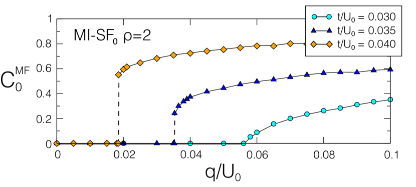
Figure 5: (Color online) Mean-field MI-SF₀ transition controlled by the $q$. Only the $\sigma=0$ component is condensed in the SF₀ phase. The jump in $C^{MF}_{0}$ is the signal of a first-order transition for $t/U_{0}=0.040$ and $t/U_{0}=0.035$, whereas the transition is second order for $t/U_{0}=0.030$.

IV Quantum Monte Carlo Phase Diagrams

We first discuss the phase diagrams, the properties of the phases with respect to the QZE, and then we focus on the quantum phase transitions.

IV.1 Phase Diagrams

For a fixed hopping $t/U_{0}$, the boundaries of the $\rho$ Mott lobe are calculated with $\mu^{+}(\rho)=E(\rho L^{2}+1)-E(\rho L^{2})$ and $\mu^{-}(\rho)=E(\rho L^{2})-E(\rho L^{2}-1)$. The charge gap $\Delta\equiv\mu^{+}-\mu^{-}$ vanishes at the tip of the Mott lobe in the thermodynamic limit.

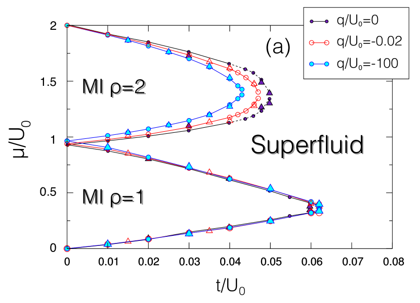
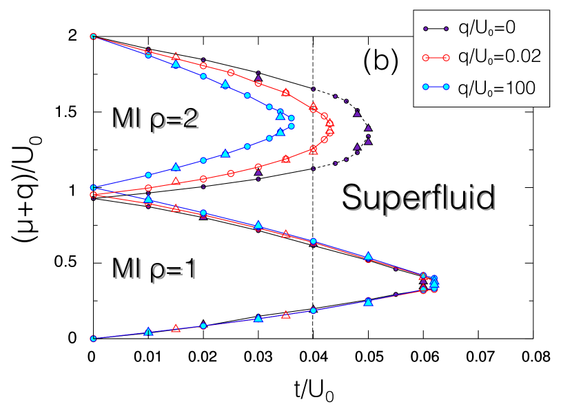
Figure 6: (Color online) QMC phase diagrams with $U_{2}/U_{0}=0.036$ for (a) negative $q$ and (b) positive $q$ values (circles: $L=8$; triangles: $L=12$). Contrary to the $\rho=1$ Mott lobe, $q$ strongly affects the tip of the $\rho=2$ Mott lobe. The dashed (plain) lines indicate a first- (second-) order transition. Contrary to the mean-field results Fig. 2, all the transitions are continuous for $q\neq 0$. The vertical dashed line in (b) at $t/U_{0}=0.04$ corresponds to the cut shown in Fig. 18.

The QMC phase diagrams are plotted in Fig. 6 for positive and negative $q$. Similar to the mean-field phase diagrams, Fig. 2, the tip of the $\rho=1$ Mott lobe does not vary with $q$, contrary to the one of the $\rho=2$ MI phase. This is because the charge gap at the tip of the $\rho=2$ Mott lobe – stabilized by the creation of pairs of bosons in the singlet state – is destroyed by $q$, thus leaving the space to the superfluid phase when increasing $|q|$. As compared to the mean field, which underestimates the quantum fluctuations, the MI lobes end at larger $t_{c}/U_{0}$ values, for all $\rho$ and $q$. Therefore, the MI regions are much bigger than the mean field ones, as expected, and the $\rho=1$ Mott phase ends at $t_{c}/U_{0}\simeq 0.06$, in agreement with the single-species Bose-Hubbard model.Capogrosso_Sansone_2008 In all the phases, we observe neither ferromagnetism, nor Néel order, i.e., no peak in magnetic structure factor $\mathcal{S}_{\alpha\alpha}({\bf k})$ [Eq. (12)] for $k=0$ and $k_{x,y}=\pi$. Nevertheless, we do observe a signal of nematic order, as discussed below.

IV.2 Densities, nematic order and MI-SF transition vs. QZE

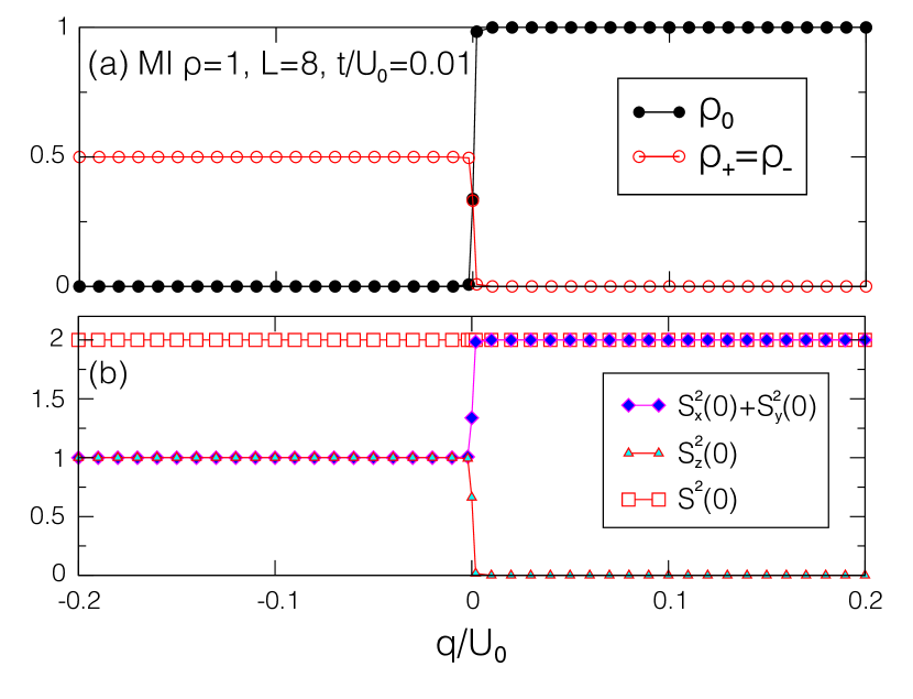
Figure 7: (Color online) QMC data in the $\rho=1$ MI phase. (a) The Zeeman term $q$ allows one to tune the populations from a state fully composed by $\sigma=\{\downarrow,\uparrow\}$ particles for $q<0$ to a full $\sigma=0$ state for $q>0$. (b) As a consequence, $q$ affects the components of the magnetic local moment, whereas its amplitude remains fixed $S^{2}(0)=2$.

We first focus on the magnetic properties of the $\rho=1$ Mott phase when varying $q$. Figure 7(a) shows the effect of the Zeeman term on the populations at fixed $t/U_{0}=0.01$. As expected, for $q<0$, the system is only composed by particles in states $\sigma=\{\downarrow,\uparrow\}$ ($\rho_{\pm}=1/2$), whereas the system is fully composed by particles in state $\sigma=0$ ($\rho_{0}=1$) for $q>0$. For $q=0$, the populations are balanced $\rho_{0}=\rho_{\pm}\simeq 1/3$. Nevertheless, for all $q$, the local magnetic moment remains fixed at $S^{2}(0)=2$; see Fig. 7(b). Therefore, the magnetic term in the Hamiltonian is constant and does not compete with the Zeeman term. Since $q$ affects the populations, the components of the local magnetic moment are also affected, see Eq. (10), such that $S^{2}_{x,y}(0)=\rho_{\pm},~{}S^{2}_{z}(0)=2\rho_{\pm}$ for $q<0$, and $S^{2}_{x,y}(0)=\rho_{0},S^{2}_{z}(0)=0$ for $q>0$, and the local magnetic moment saturates to its maximal value $S^{2}(0)=2\rho,\forall q$.deforges2014 A finite local magnetic moment is a necessary but not sufficient condition for the establishment of a magnetic ordering, and we should carefully look at the nematic correlation functions.DeChiara_2011

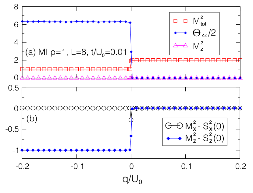
Figure 8: (Color online) QMC data in the $\rho=1$ MI phase. (a) $\Theta_{zz}\neq 0$ and $M^{2}_{z}=0$ are indicators of a nematic order along $z$. (b) The nematic order along $z$ implies $M^{2}_{z}-S_{z}^{2}(0)<0$. In the $xy$ plane, we observe nonvanishing correlation $M^{2}_{x,y}-S_{x,y}^{2}(0)\neq 0$ only for $q=0$.

The magnetic correlation functions are plotted in Fig. 8. The nematic order parameter $\Theta_{zz}\neq 0$ is non zero for $q\leq 0$; see Fig. 8(a). Indeed, a nematic order along $z$ is consistent with a vanishing magnetization $M^{2}_{z}=0$,deforges2014 ; Katsura and non vanishing correlation $M^{2}_{z}-S_{z}^{2}(0)=\frac{1}{L^{4}}\sum_{\bf r,R\neq 0}\langle{\hat{S}}_{z,{\bf r}}{\hat{S}}_{z,{\bf r+R}}\rangle\neq 0$ observed in Fig. 8(b). In the $xy$ plane, we only observe non vanishing correlation functions for $q=0$ for which $M^{2}_{x,y}-S_{x,y}^{2}(0)\neq 0$. In conclusion, we observe a nematic phase for $q\leq 0$.

The situation is very different in the $\rho=2$ Mott phase since the local magnetic moment is fully minimized, i.e., $S^{2}(0)=0$, in the $t/U_{0}\to 0$ limit. Therefore, the local magnetic moment $S^{2}(0)$ and the Zeeman term are in competition for minimizing the free energy of Hamiltonian Eq. (1). Similarto Fig. 7(a), the system is only composed by particles in states $\sigma=\{\downarrow,\uparrow\}$ ($\rho_{\pm}=1$) for $q/U_{0}\to-\infty$, whereas the system is fully composed by particles in state $\sigma=0$ ($\rho_{0}=2$) for $q/U_{0}\to+\infty$; see Fig. 9(a). Nevertheless, contrary to the $\rho=1$ case plotted in Fig. 7(a), we observe a smooth crossover at $q=0$ for which the system adopts a singlet state such that $\rho_{sg}=1$ and $S^{2}(0)=0$; see Fig. 9(b).

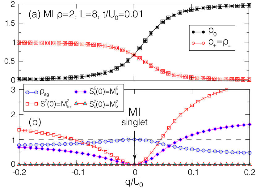
Figure 9: (Color online) QMC data in the $\rho=2$ MI phase. (a) The Zeeman term $q$ tunes the populations from a state fully composed by $\sigma=\{\downarrow,\uparrow\}$ particles for $q\to-\infty$ to a full $\sigma=0$ state for $q\to+\infty$. For $q=0$, the system adopts a singlet state with balanced populations. Squares are the densities calculated using the local wave function Eq. (18). (b) The magnetic correlations are absent since $M^{2}_{\rm tot}-S^{2}(0)=0,\forall q$.

For $q\neq 0$, the minimization of the Zeeman term breaks the singlet state which leads to a non vanishing local moment $S^{2}(0)\neq 0$ in the plane $xy$, i.e., $S_{x,y}^{2}(0)\neq 0$, but with $S_{z}^{2}(0)=0$. These local quantities are well described by the on-site wave function Eq. (18). Clearly, $|\Phi_{\rho=2,q\to-\infty}\rangle=|1,0,1\rangle$ leads to $\rho_{\pm}=1$, and $|\Phi_{\rho=2,q\to+\infty}\rangle=-|0,2,0\rangle$ leads to $\rho_{0}=2$. For $q=0$, the singlet state $|\Phi_{\rho=2,q=0}\rangle=\frac{1}{\sqrt{3}}\left(\sqrt{2}|1,0,1\rangle-|0,2,0\rangle\right)$ leads to $\rho_{\pm}=\rho_{0}=2/3$ and $\langle a_{0{\bf r}}^{\dagger}a_{0{\bf r}}^{\dagger}a_{\uparrow{\bf r}}^{\phantom{\dagger}}a_{\downarrow{\bf r}}^{\phantom{\dagger}}\rangle=-2/3$ from Eq. (10). The finite local moment obtained for $q\neq 0$ may suggest a magnetic ordering in the $xy$ plane, since $S^{2}_{x,y}(0)-\frac{1}{3}S^{2}(0)\neq 0$.Imambekov_2004 ; demler02 In fact, the contribution of the spin-spin correlation functions, when removing the auto-correlation contribution, vanishes, i.e., $M^{2}_{\rm tot}-S^{2}(0)=\frac{1}{L^{4}}\sum_{\sigma,\bf r,R\neq 0}\langle{\hat{S}}_{\sigma,{\bf r}}{\hat{S}}_{\sigma,{\bf r+R}}\rangle=0$. Therefore, there is no magnetic order for $t/U_{0}=0.01$ in the $\rho=2$ Mott phase $\forall q$.

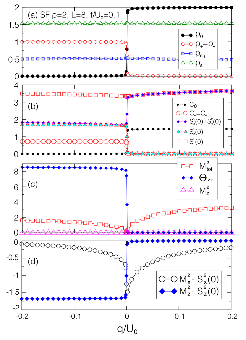
Figure 10: (Color online) QMC data in the $\rho=2$ SF phase with $L=8$: (a) the superfluid and singlet densities $\rho_{s}$, $\rho_{sg}$ are insensitive to $q$. (b) The condensate is supported by $\sigma=\{\downarrow,\uparrow\}$ ($\sigma=0$) bosons for $q<0$ ($q>0$) and the $z$ component of local magnetic moment $S_{z}^{2}(0)$ vanishes for $q>0$ due to $\rho_{\pm}=0$. (c),(d) The magnetic moment $M^{2}_{\rm tot}$ vanishes for $q=0$ and we observe a nematic order along $z$ only for $q\leq 0$ ($\Theta_{zz}\neq 0$) associated with negative correlations $M^{2}_{z}-S_{z}^{2}(0)<0$. In the $xy$ plane, the amplitude of the spin-spin correlations $|M^{2}_{x,y}-S_{x,y}^{2}(0)|$ reaches its maximum for $q=0$ and vanishes for $q\to\pm\infty$.

We now focus on the $\rho=2$ superfluid phase, in which the kinetic term is dominant: the Bose-Einstein condensation – associated with the spontaneous U(1) symmetry breaking – occurs; hence $\rho_{s}\neq 0$ and $C_{\sigma}\neq 0$. Therefore, the QZE also affects the condensate populations $C_{\sigma}$. As an example, we focus on the case with $t/U_{0}=0.1$; see Fig. 10. The superfluid density $\rho_{s}$ and singlet density $\rho_{sg}$ do not significantly vary with $q$, whereas the populations evolve from a state fully composed by $\sigma=\{\downarrow,\uparrow\}$ particles for $q\to-\infty$ to a full $\sigma=0$ state for $q\to+\infty$ [Fig. 10(a)]. Note that the redistribution of the population at $q=0$ is sharp – similar to the $\rho=1$ MI phase in Fig. 7(a). This is because the spin-spin interaction term in Eq. (1) is now in competition with a dominant kinetic term and has a smaller effective strength. The condensates $C_{\sigma}$ naturally follow the densities $\rho_{\sigma}$ [Fig. 10(b)]. The components of the local magnetic moment behave qualitatively in the same way as in the $\rho=1$ Mott phase, Fig. 10(b), but do not reach their maximal values since a small fraction of particles remains in the singlet state for $t/U_{0}=0.1$, that is $S^{2}_{x,y}(0)<\rho_{\pm},~{}S^{2}_{z}(0)<2\rho_{\pm}$ for $q<0$, and $S^{2}_{x,y}(0)<\rho_{0}$ for $q>0$; hence $S^{2}(0)<2\rho,\forall q$deforges2014 (or equivalently $\langle a_{0{\bf r}}^{\dagger}a_{0{\bf r}}^{\dagger}a_{\uparrow{\bf r}}^{\phantom{\dagger}}a_{\downarrow{\bf r}}^{\phantom{\dagger}}\rangle<0$). Compared to the $\rho=1$ Mott phase, the director of the nematic order in the $\rho=2$ superfluid can belong to the three axes in a larger range of $q$: the signal of a nematic phase along $z$ is clearly observed in Fig. 10(c) where $\Theta_{zz}\neq 0$ for $q\leq 0$. This statement is strengthened by the non vanishing correlation function $M^{2}_{z}-S_{z}^{2}(0)<0$ in Fig. 10(d). Nevertheless, $\Theta_{zz}=0$ for $q>0$ indicates a vanishing nematic order along $z$. Furthermore, in the $xy$ plane, the amplitude of the spin-spin correlations $|M^{2}_{x,y}-S_{x,y}^{2}(0)|$ reaches its maximum for $q\simeq 0$ and vanishes for $q\to\pm\infty$. Interestingly enough, the nematic correlations $|M^{2}_{\rm tot}-S^{2}(0)|$ are maximized when the global magnetism $M^{2}_{\rm tot}$ vanishes at $q=0$ [Fig. 10(c)]. Our results are in good agreement with previous studiesKatsura ; Deforges_2013 ; deforges2014 which have predicted a nematic order in the superfluid phase with broken SU(2) symmetry. In the limit $U_{2}\ll t$, with $U_{0}=q=0$ and $\rho=2$, the nematic correlations take the exact value $M^{2}_{\rm tot}-S^{2}(0)=-2\rho=-4$.deforges2014 With the data of Fig. 10, we obviously find a smaller value $|M^{2}_{\rm tot}-S^{2}(0)|\simeq 3.3$ because of the non-negligible interactions $U_{0}=10~{}t$ which allow the formation of a small fraction of particles in the singlet state, hence $\langle a_{0{\bf r}}^{\dagger}a_{0{\bf r}}^{\dagger}a_{\uparrow{\bf r}}^{\phantom{\dagger}}a_{\downarrow{\bf r}}^{\phantom{\dagger}}\rangle<0$ from Eq. (10), thus partially destroying the nematic order. In conclusion, the director of the nematic order evolves form a director along $z$ for $q\to-\infty$ to a director with finite $xyz$ components at $q\simeq 0$. For $q>0$, the director belongs to the $xy$ plane and the nematic order disappears as $q$ is increased.

For intermediate $t/U_{0}$, the QZE can act as a control parameter of the Mott-superfluid transition as shown at the mean field level in Fig. 4. This effect is confirmed by our QMC simulations for $t/U_{0}=0.045$, where the system adopts a Mott phase for $q/U_{0}\in[-0.045,0.01]$ with $\rho_{s}=0$ and is superfluid $\rho_{s}\neq 0$ otherwise; see Fig. 11(a).

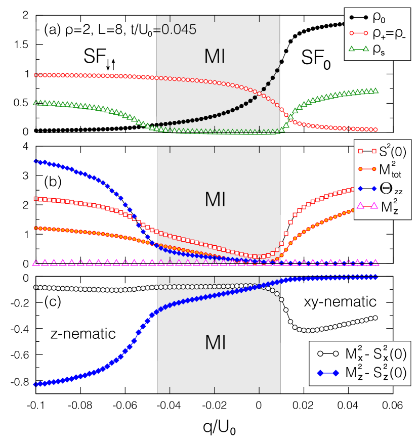
Figure 11: (Color online) QMC data for $\rho=2$ and $L=8$ at fixed hopping $t/U_{0}=0.045$: $q$ acts as a control parameter for the MI-SF transition. For $q\to-\infty$ the system is in the SF_↓↑ with a nematic director along $z$ axis and enters in the MI phase at $q/U_{0}\simeq-0.045$ when increasing $q$. Then, the system continuously adopts a SF₀ phase with a nematic director belonging to the $xy$ plane at $q/U_{0}\simeq 0.01$. Both transitions are second order.

In agreement with the mean-field results, the densities evolve from $\rho_{\pm}=1$ for $q/U_{0}\to-\infty$ to $\rho_{0}=2$ for $q/U_{0}\to+\infty$, and $\rho_{\pm}=\rho_{0}=2/3$ at $q/U_{0}=0$ where the local magnetic moment $S^{2}(0)$ and the magnetization $M^{2}_{\rm tot}$ are minimized; see Fig. 11(b). Although the magnetization is strictly zero along the $z$ axis, i.e., $M^{2}_{z}=0$, we observe a clear signal of a nematic order along the $z$ axis in the SF_↓↑ phase, i.e., $\Theta_{zz}\neq 0$; see Fig. 11(b). Furthermore, we observe nematic correlation $M^{2}_{z}-S_{z}^{2}(0)<0$ in the SF_↓↑ phase, Fig. 11(c). In the SF₀ phase for $q/U_{0}>0.01$, the nematic order is developed in the $xy$ plane, where $M^{2}_{x,y}-S_{x,y}^{2}(0)<0$; see Fig. 11(c). Therefore, the QZE allows one to control both the phase coherence and the director of the nematic order. Contrary to the mean-field predictions, our data for $L=8,10$ show continuous transitions.

IV.3 Nature of the $\rho=1,2$ MI-SF transitions

Our mean-field results, Fig. 3, suggest that the nature of the MI-SF transition varies with $q$ for $\rho=2$, whereas it remains second order for $\rho=1$. We now use the QMC method for investigating this effect.

Similar to Fig. 3, the critical hopping $t_{c}/U_{0}$ at the transition is highly sensitive to $q$ for $\rho=2$, but does not change for $\rho=1$; see Fig. 12.

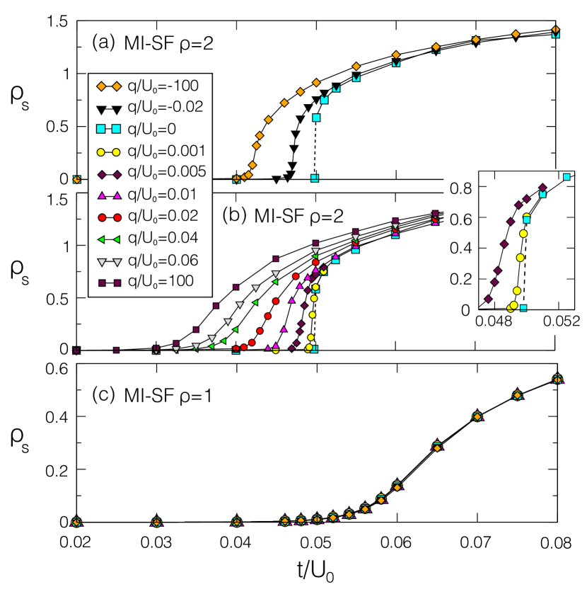
Figure 12: (Color online) QMC data of the superfluid density $\rho_{s}$ at the MI-SF transition with $L=8$ for $\rho=2$ with (a) negative $q$ and (b) positive $q$, and (c) for $\rho=1$, $\forall q$. Contrary to the $\rho=2$ case, $\rho_{s}$ does not depend on $q$ for $\rho=1$. We only observe a discontinuity in $\rho_{s}$ for $\rho=2$ and $q=0$, and the transition is first order; see zoom inset panel (b).

These different behavior comes from the possible minimization of $S^{2}(0)$ for $\rho=2$, whereas $S^{2}(0)=2,\forall q$ for $\rho=1$. Therefore, the minimization of the free energy of the Hamiltonian Eq. (1) leads to a competition between the Zeeman term and the minimization of $S^{2}(0)$ only for $\rho=2$. However, the QMC and mean-field predictions are in contradictions: our QMC simulations explicitly indicate a first-order transition – signaled by a jump in $\rho_{s}$ in Figs. 12(a) and 12(b) – only for $q/U_{0}=0$. Indeed, even for very small $q$ values, e.g., $q/U_{0}=0.001$, the jump in $\rho_{s}$ vanishes, suggesting a second order transition.

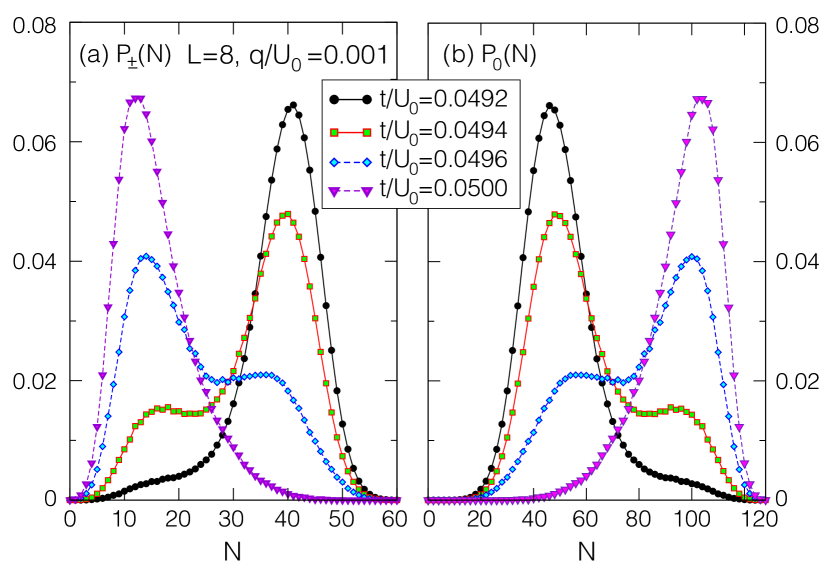
Figure 13: (Color online) QMC data with $L=8$, $\rho=2$, and $q/U_{0}=0.001$. The density histograms (a) $P_{\pm}(N)$ and (b) $P_{0}(N)$ show a double peak structure close to the transition at $t/U_{0}=0.0494$ and $t/U_{0}=0.0496$, thus indicating a weak first-order transition.

Nevertheless, the density histograms plotted in Fig. 13 show double peaks at the transition ($t_{c}/U_{0}\simeq 0.0494$), thus indicating a weak first-order transition for $q/U_{0}=0.001$. A similar signal is observed for $q/U_{0}=-0.005$ but disappears for $q/U_{0}<-0.005$ and $q/U_{0}>0.001$. Therefore, the transition is found to be first-order only for $q/U_{0}\in[-0.005,0.001]$.

The nature of the $\rho=2$ MI-SF transition is also determined by using finite-size scaling analysis; see Fig. 14.

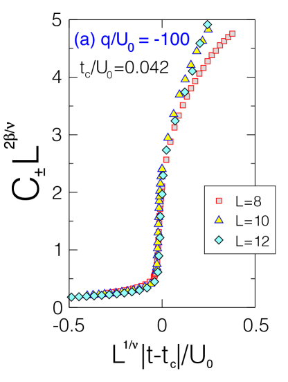
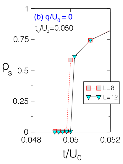
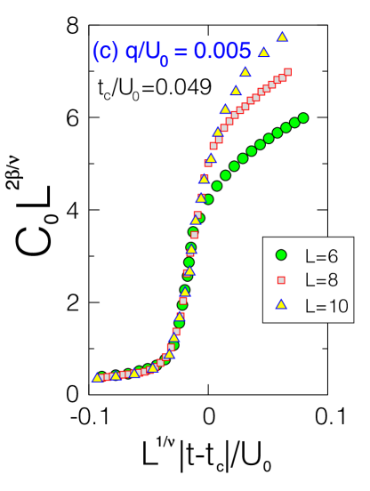
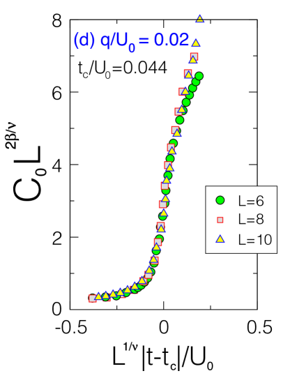
Figure 14: (Color online) QMC scaling plots of the $\rho=2$ MI-SF transition for (a) $q/U_{0}=-100$, (b) $q/U_{0}=0$, (c) $q/U_{0}=0.005$, and (d) $q/U_{0}=0.02$. For $q\neq 0$, the scaling of the condensate fractions $C_{0},C_{\pm}$ are consistent with a transition of the 3D XY nature, even for small $q/U_{0}$ (c). Critical exponents of the 3D XY universality classes are used for the scaling, i.e., $\beta=0.3479$ and $\nu=0.6706$.Pelissetto_2002 The jump observed in $\rho_{s}$ for $q=0$ (b) indicates a first-order transition.Deforges_2013 ; pai08

For $q=0$, the jump in $\rho_{s}$ remains finite for many sizes; see Fig. 14(b), strengthening the conclusion of a first-order transition associated with the symmetry breaking of both U(1) and SU(2). This transition has been previously investigatedDeforges_2013 ; pai08 and other signatures of a first-order transition have been found using QMC simulations (e.g., see Fig. 16 of Ref. Deforges_2013 ). For $q/U_{0}\notin[-0.005,0.001]$, the transition is found to be of the 3D XY nature; see Figs. 14(a), 14(c), and 14(d). This result is not surprising in the limit $q/U_{0}\to+\infty$ since only the component $\sigma=0$ is populated, thus leading to a single species Bose-Hubbard model. However, this result is more surprising for small positive $q/U_{0}$ and for large negative $q/U_{0}$, since a nematic order is established at the MI-SF transition, thus potentially changing the nature of the transition, as observed for $q/U_{0}=0$.

IV.4 Nematic order at the $\rho=2$ MI-SF transition with fixed $q/U_{0}$

We now investigate the establishment of the nematic order at the $\rho=2$ MI-SF transition for large and zero $|q|$ values. To fix the idea, we begin with the simplest case, $q\to+\infty$, for which we recover the single species Bose-Hubbard model with $\rho_{0}=2$ and $\rho_{\pm}=0$; see Fig. 15 for which $q/U_{0}=100$.

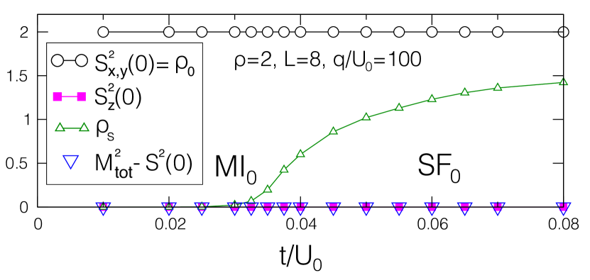
Figure 15: (Color online) QMC data of the $\rho=2$ MI-SF transition with $L=8$ and $q/U_{0}=100$. The system behaves like the standard single species Bose-Hubbard model with $\rho_{0}=2$, for which the transition belongs to the 3D XY universality class,Fisher_1989 without magnetic order $M^{2}_{\rm tot}-S^{2}(0)=0$.

Since $\rho_{\pm}=0$, the local magnetic moment along $z$ trivially vanishes, $S_{z}^{2}(0)=0$, whereas $S_{x,y}^{2}(0)=\rho_{0}$ is saturated; see Eq. (10). Obviously, there is no magnetic order, $M^{2}_{\rm tot}-S^{2}(0)=0,\forall q$.Blume_Capel

In the other limit, $q/U_{0}\to-\infty$, the situation is very different since the establishment of the phase coherence leads to the establishment of the nematic order. In this limit, the densities read $\rho_{\pm}=1$ and $\rho_{0}=0$, $\forall q$, and the system undergoes a phase transition from a MI_↑↓ to a SF_↑↓. According to Eq. (10), this leads to a saturated local magnetic moment in the $xy$ plane such that $S^{2}_{x,y}(0)=\rho_{\pm}$, whereas a spin degree of freedom remains along the $z$ axis. In this case, the magnetic SU(2) symmetry reduces to the $\mathbb{Z}_{2}$ Ising symmetry. For $t/U_{0}\to 0$, the Mott phase is described by the on-site wave function $|\Phi_{\rho=2,q\to-\infty}\rangle=|1,0,1\rangle$ ensuring $S_{z}^{2}(0)=0$. These results are observed for $q/U_{0}=-100$ in Fig. 16 (a).

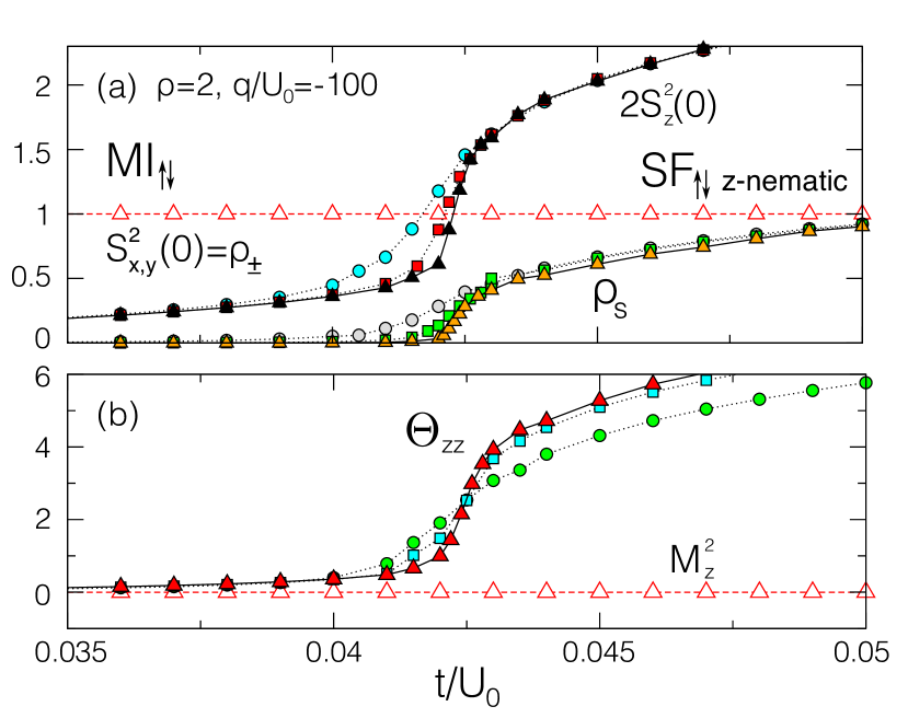
Figure 16: (Color online) QMC data for the $\rho=2$ MI-SF transition for $q/U_{0}=-100$ with $L=6$ (circles), 8 (squares), and 10 (triangles). We observe a continuous transition at $t_{c}/U_{0}=0.042$ from a MI_↑↓ ($\rho_{s}=0,\Theta_{zz}=0$) to a nematic SF_↑↓ with a director along $z$ ($\rho_{s}\neq 0,\Theta_{zz}\neq 0$).

When increasing $t/U_{0}$, the $z$ component of the magnetic local moment $S^{2}_{z}(0)$ significantly increases when the phase coherence is established $\rho_{s}\neq 0$, at $t_{c}/U_{0}=0.042$. Indeed, the phase coherence involves density fluctuations which prevents the full minimization of $S^{2}_{z}(0)$. Nevertheless, the magnetization $M^{2}_{z}$ remains zero for all $t/U_{0}$; see Fig. 16(b). Furthermore, the nematic order parameters $\Theta_{zz}$ becomes finite at $t_{c}/U_{0}\simeq 0.042$, thus indicating the establishment of a nematic order along $z$ associated with nematic correlations $M^{2}_{z}-S_{z}^{2}(0)=\frac{1}{L^{4}}\sum_{\bf r,R\neq 0}\langle{\hat{S}}_{z,{\bf r}}{\hat{S}}_{z,{\bf r+R}}\rangle\neq 0$ in the superfluid phase. We observe a scaling of $\Theta_{zz}$ consistent with the 3D Ising universality class, using exponents $\beta=0.3265$ and $\nu=0.6301$Pelissetto_2002 (not shown). In conclusion, we observe a continuous transition with broken U(1)$\times\mathbb{Z}_{2}$ symmetries from a MI phase to a nematic SF with a director along $z$.

Finally, we discuss the case $q=0$. The main difference with the previous cases is that the nematic order could be established along the three axes in the superfluid phase. In the $t/U_{0}\to 0$ limit, the singlet MI is described by the singlet wave function $|\Phi_{\rho=2,q=0}\rangle=\frac{1}{\sqrt{3}}\left(\sqrt{2}|1,0,1\rangle-|0,2,0\rangle\right)$ with $\rho_{\rm sg}=1$, $\rho_{\pm}=\rho_{0}=2/3$, and $S_{\alpha}^{2}(0)=0$; see Fig. 17.

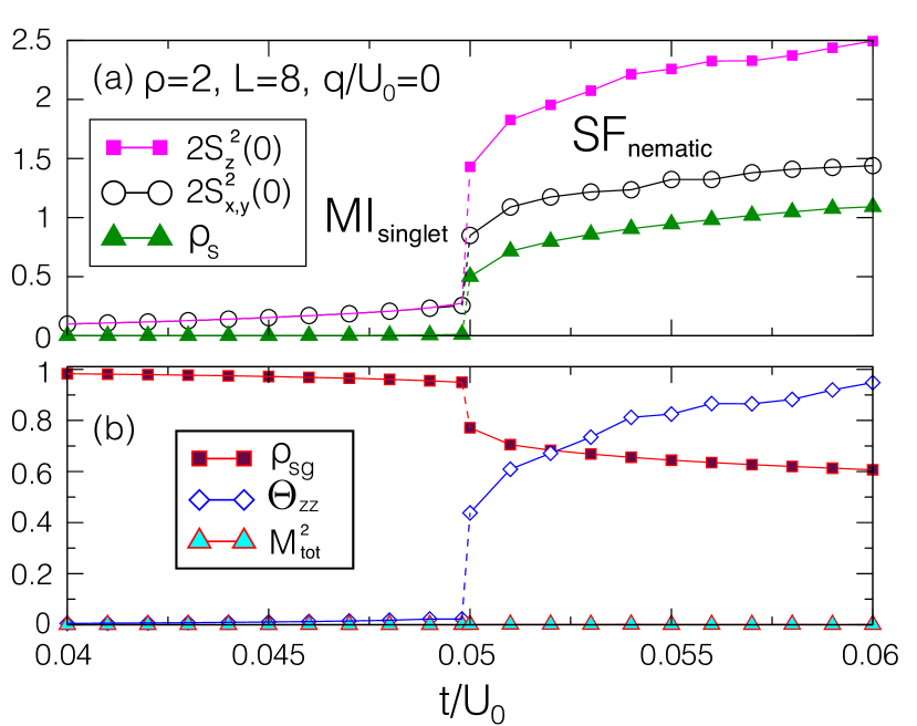
Figure 17: (Color online) QMC data for the $\rho=2$ MI-SF transition for $q/U_{0}=0$ and $L=8$. The system undergoes a first-order transition – indicated by a jump in the quantities – from a singlet Mott insulator to a fully nematic superfluid.

The jump in $\rho_{s}$ discussed in Fig. 14(b) is also observed in the component of the local magnetic moment $S^{2}_{\alpha}(0)$, which becomes finite in the three axes $x,y,z$ at the transition at $t_{c}/U_{0}\simeq 0.05$ [Fig. 17(a)]. Furthermore, the singlet density $\rho_{\rm sg}$ and the nematic order parameter $\Theta_{zz}$ also jump at the transition, whereas the global magnetization $M^{2}_{\rm tot}$ remains zero; see Fig. 17(b). Therefore, the nematic order and the phase coherence are simultaneously established when the hopping $t/U_{0}$ is strong enough to destroy the singlet state. Since $M^{2}_{\rm tot}=0$ and $S^{2}_{\alpha}(0)\neq 0$ $\forall\alpha$ in the superfluid phase, it is clear that the nematic correlations are finite along the three axes, $M^{2}_{\alpha}-S_{\alpha}^{2}(0)<0$ with $\alpha=\{x,y,z\}$. In conclusion, the system undergoes a first-order transition from a singlet MI to a fully nematic SF.

IV.5 Vertical slice of the phase diagram

To complete the picture, we discuss a vertical slice in the phase diagram Fig. 6(b). Figure 18 shows such a slice at $t/U_{0}=0.04$ for three values of $q/U_{0}$. For $q=0$, the first and second Mott lobes are indicated by the plateaus $\rho=1,2$, with a vanishing superfluid density $\rho_{s}=0$; see Fig. 18(a).

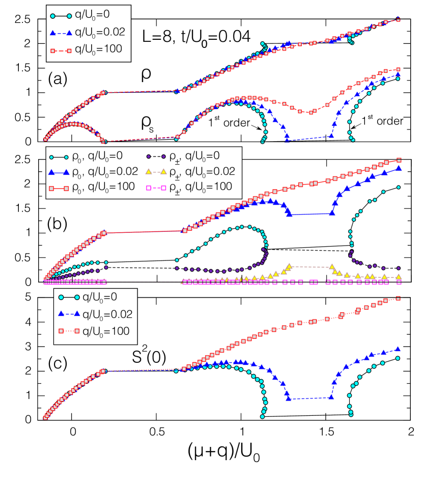
Figure 18: (Color online) QMC data of the vertical slice of phase diagram Fig. 6(b) at fixed hopping $t/U_{0}=0.04$ for $q/U_{0}=\{0,0.02,100\}$. (a) Total density $\rho$, and superfluid density $\rho_{s}$, (b) densities of each Zeeman state $\rho_{\sigma}$, and (c) total magnetic local moment $S^{2}(0)$ as function of $\mu$.

When turning on the QZE, the $\rho=2$ Mott gap reduces (e.g., $q/U_{0}=0.02$) and disappears for strong enough $q$ (e.g., $q/U_{0}=100$), thus leaving space to a superfluid phase $\rho_{s}\neq 0$. This effect is not observed for the $\rho=1$ Mott gap. The density $\rho_{0}$ increases with $q$ and saturates at $\rho_{0}=\rho$ for very large $q$ (e.g., $q/U_{0}=100$); see Fig. 18(b). Nevertheless, for $q/U_{0}=0.02$, we still observe a mixing in the populations close to the $\rho=2$ Mott plateau due to the minimization of $S^{2}(0)$ which forms singlet state pairs, and therefore populates the $\sigma=\{\downarrow,\uparrow\}$ states. Furthermore, the competition between the QZE and the spin-spin interaction is shown in Fig. 18 (c): for $\rho>1$, the formation of singlet states is activated for $q=0$, thus leading to the minimization of the local magnetic moment such that $S^{2}(0)\sim 0$ in the $\rho=2$ Mott phase [$S^{2}(0)$ does not strictly vanish for $t/U_{0}=0.04$ since the hopping term destroys a small fraction of singlet pairs]. For $q/U_{0}=0.02$, the singlet pairs are partially destroyed by the QZE and $S^{2}(0)$ takes a non vanishing value in the $\rho=2$ Mott phase. For very large $q$ (e.g., $q/U_{0}=100$), for which $\rho_{0}=\rho$, it is not possible to form singlet state anymore and the magnetic local moment saturates $S^{2}(0)=2\rho$; see Eq. (10).

Concerning the quantum phase transitions, our QMC simulations predict continuous transitions, except for the $\rho=2$ MI-SF transitions with $q=0$: the negative slope in $\rho$ versus $\mu$ indicates a negative compressibility since $\kappa=\partial\rho/\partial\mu<0$, thus indicating a metastable region. This signal, which is a well-know signature of a first-order transition in the canonical ensemble, batrouni2000 ; Deforges_2013 ; Deforges_2011 is also observed in other quantities, e.g., $\rho_{\alpha},\rho_{s}$, and $S^{2}(0)$. These QMC results for $q=0$ are in good qualitative agreement with mean field results of Fig. 1. Nevertheless, these two approaches give incompatible predictions concerning the nature of the $\rho=2$ MI-SF transition for finite $q$: According to the mean-field approach, the $\rho=2$ MI-SF transition should be first order for $q/U_{0}=0.02$. However, the first-order signature is not observed for $q/U_{0}=0.02$ with QMC simulation, for which the $\rho=2$ MI-SF transition is continuous; see Fig. 18.

V Conclusions

Employing quantum Monte Carlo simulations and mean-field theory, we derived the phase diagram of interacting lattice spin-1 bosons subject to the QZE. The interactions are among the simplest possible for such a system: an on-site repulsion independent of spin and an on-site antiferromagnetic coupling between spins on the same site. The QZE splits the energy of the sublevels $\sigma=\pm 1$ and $\sigma=0$.

We have particularly focused on the magnetic properties of the Mott and superfluid phases, and on the Mott-superfluid transition when varying the Zeeman splitting. In the absence of QZE, the antiferromagnetic interactions lead to the establishment of a nematic state – i.e., a state breaking spin-rotation symmetry without magnetic order – in the superfluid phase and in the Mott phases with odd filling, whereas the system adopts a singlet state with zero magnetic local moment in even Mott lobes.Deforges_2013 Both quantum Monte Carlo simulations and mean-field theory show that the QZE, which directly impacts the populations of $\sigma=\{\pm 1,0\}$ states, destroys the singlet state at the tip of the even Mott lobes, thus leaving the space to the superfluid phase. This effect is not observed in the Mott lobes with one particle per site since the system cannot form a singlet state. Therefore, the QZE acts as a control parameter for the MI-SF transition with even filling and fixed hopping, as observed in a cubic lattice.Liu_2016 Our present study goes beyond the mean-field approximation since quantum Monte Carlo simulations give access to magnetic correlation functions required for a reliable definition of a nematic order parameter. We found a spin nematic order with director along the $z$ axis in the odd Mott lobes and in the superfluid phase for favored $\sigma=\pm 1$ states, whereas the $xy$ components of the nematic director remain finite for moderate QZE in the superfluid phase with even filling. We also elucidate the nature of the quantum phase transitions: the Mott-superfluid transition with even filling is found to be first order for $q/U_{0}\in[-0.005,0.001]$ and is 3D XY otherwise, contrary to the mean field approach which predicts a first-order transition in a larger range, for $q/U_{0}\leq 0.04$. Our study clearly shows that the QZE is a control parameter for both the nematic structure and for the MI-SF transition. This phenomenology sets the stage for future experiments on spinor condensates in optical lattices, using state-of-the-art techniques.Zibold_2016 ; Trotzky_2010 ; Liu_2016

- (1) D. Jaksch, C. Bruder, J. I. Cirac, C. W. Gardiner, and P. Zoller, Phys. Rev. Lett. 81, 3108 (1998).
- (2) M. Greiner, O. Mandel, T. Esslinger, T.W. Hänsch, and I. Bloch, Nature 415, 39 (2002).
- (3) M. P. A. Fisher, P. B. Weichman, G. Grinstein, and D. S. Fisher, Phys. Rev. B 40, 546 (1989).
- (4) I. Bloch, J. Dalibard, and W. Zwerger, Rev. Mod. Phys. 80, 885 (2008).
- (5) J. K. Chin, D. E. Miller, Y. Liu, C. Stan, W. Setiawan, C. Sanner, K. Xu, and W. Ketterle, Nature 443, 961 (2006).
- (6) U. Schneider, L. Hackermüller, S. Will, Th. Best, I. Bloch, T. A. Costi, R. W. Helmes, D. Rasch, and A. Rosch, Science 322, 1520 (2008).
- (7) R. Jördens, N. Strohmaier, K. Günter, H. Moritz, and T. Esslinger, Nature 455, 204 (2008).
- (8) J. Dalibard, F. Gerbier, G. Juzeliunas, and P. Öhberg, Rev. Mod. Phys. 83, 1523 (2011).
- (9) D. M. Stamper-Kurn and M. Ueda, Rev. Mod. Phys. 85, 1191 (2013).
- (10) F. Gerbier, A. Widera, S. Fölling, O. Mandel, and I. Bloch, Phys. Rev. A 73, 041602(R) (2006).
- (11) L. Zhao, J. Jiang, T. Tang, M. Webb, and Y. Liu, Phys. Rev. Lett. 114, 225302 (2015).
- (12) Y. Kawaguchi and M. Ueda, Rep. Prog. Phys. 77, 122401 (2014).
- (13) K. V. Krutitsky, Physics Reports 607, 1-101 (2016).
- (14) M. Lewenstein and A. Sanpera, Science 319, 292 (2008).
- (15) M.-S. Chang, Q. Qin, W. Zhang, L. You, and M. S. Chapman, Nature Physics 1, 111-116 (2005).
- (16) A. B. Kuklov and B.V. Svistunov, Phys. Rev. Lett. 90, 100401 (2003).
- (17) A. Lamacraft, Phys. Rev. B 81, 184526 (2010).
- (18) J. Jiang, L. Zhao, S.-T. Wang, Z. Chen, T. Tang, L.-M. Duan, and Y. Liu, Phys. Rev. A 93, 063607 (2016).
- (19) J. Estève, C. Gross, A. Weller, S. Giovanazzi, and M. K. Oberthaler, Nature 455, 1216-1219 (2008).
- (20) D. M. Weld, P. Medley, H. Miyake, D. Hucul, D. E. Pritchard, and W. Ketterle, Phys. Rev. Lett. 103, 245301 (2009); F. Lingua, B. Capogrosso-Sansone, F. Minardi, and V. Penna, Sci. Rep. 7, 5105 (2017).
- (21) M. A. Alpar, S. A. Langer, and J. A. Sauls, Astrophys. J. 282, 533-541 (1984); M. Lattimer and M. Prakash, Science 304, 536 (2004).
- (22) M. Tylutki, L. P. Pitaevskii, A. Recati, and S. Stringari, Phys. Rev. A 93, 043623 (2016); D. T. Son, M. A. Stephanov, and A. R. Zhitnitsky, Phys. Rev. Lett. 86, 3955 (2001); D. T. Son and M. A. Stephanov, Phys. Rev. A 65, 063621 (2002).
- (23) M. Vengalattore, S. R. Leslie, J. Guzman, and D. M. Stamper-Kurn, Phys. Rev. Lett. 100, 170403 (2008).
- (24) M. Vengalattore, J. Guzman, S. R. Leslie, F. Serwane, and D. M. Stamper-Kurn, Phys. Rev. A 81, 053612 (2010).
- (25) T. Ohmi and K. Machida, J. Phys. Soc. Jpn. 67, 1822 (1998).
- (26) T.-L. Ho, Phys. Rev. Lett. 81, 742 (1998).
- (27) B. Capogrosso-Sansone, S. G. Söyler, N. V. Prokofév and B. V. Svistunov, Phys. Rev. A 81, 053622 (2010).
- (28) A. Imambekov, M. Lukin, and E. Demler, Phys. Rev. A 68, 063602 (2003) and Phys. Rev. Lett. 93, 120405 (2004).
- (29) M. Snoek and F. Zhou, Phys. Rev. B 69, 094410 (2004).
- (30) L. de Forges de Parny, F. Hébert, V. G. Rousseau, and G. G. Batrouni, Phys. Rev. B 88, 104509 (2013).
- (31) L. de Forges de Parny, H-Y. Yang, and F. Mila, Phys. Rev. Lett. 113, 200402 (2014).
- (32) L. de Forges de Parny, V.G. Rousseau, and T. Roscilde, Phys. Rev. Lett. 114, 195302 (2015).
- (33) L. de Forges de Parny, A. Rançon, and T. Roscilde. Phys. Rev. A 93, 023639 (2016).
- (34) M. Theis, G. Thalhammer, K. Winkler, M. Hellwig, G. Ruff, R. Grimm, and J. H. Denschlag, Phys. Rev. Lett. 93, 123001 (2004); C. Chin, R. Grimm, P. Julienne, and E. Tiesinga Rev. Mod. Phys. 82, 1225 (2010).
- (35) D. M. Stamper-Kurn and W. Ketterle, in Coherent Atomic Matter Waves, edited by R. Kaiser, C. Westbrook, and F. David (Springer, Berlin, 2001), p. 137.
- (36) R. V. Pai, K. Sheshadri, and R. Pandit, Phys. Rev. B 77, 014503 (2008).
- (37) T. Kimura, S. Tsuchiya, and S. Kurihara, Phys. Rev. Lett. 94, 110403 (2005).
- (38) K. V. Krutitsky and R. Graham, Phys. Rev. A 70, 063610 (2004).
- (39) Y. Li, L. He, and W. Hofstetter, Phys. Rev. A 93, 033622 (2016).
- (40) Y. Toga, H. Tsuchiura, M. Yamashita, K. Inaba, and H. Yokoyama, J. Phys. Soc. Jpn. 81, 063001 (2012).
- (41) H. Katsura and H. Tasaki, Phys. Rev. Lett. 110, 130405 (2013).
- (42) E. Demler and F. Zhou, Phys. Rev. Lett. 88, 163001 (2002).
- (43) T. Kimura, Phys. Rev. A 87, 043624 (2013).
- (44) M. Rizzi, D. Rossini, G. De Chiara, S. Montangero, and R. Fazio, Phys. Rev. Lett. 95, 240404 (2005).
- (45) S. Bergkvist, I. P. McCulloch, and A. Rosengren, Phys. Rev. A 74, 053419 (2006).
- (46) V. Apaja and O. F. Syljuåsen, Phys. Rev. A 74, 035601 (2006).
- (47) G. G. Batrouni, V. G. Rousseau, and R. T. Scalettar, Phys. Rev. Lett. 102, 140402 (2009).
- (48) N. Kawashima, Prog. Theor. Phys. Suppl. 145, 138 (2002).
- (49) S. Tsuchiya, S. Kurihara, and T. Kimura, Phys. Rev. A 70, 043628 (2004).
- (50) G. De Chiara, M. Lewenstein, and A. Sanpera, Phys. Rev. B 84, 054451 (2011).
- (51) F. Zhou, M. Snoek, J. Wiemer, and I. Affleck, Phys. Rev. B 70, 184434 (2004).
- (52) T. Zibold, V. Corre, C. Frapolli, A. Invernizzi, J. Dalibard, and F Gerbier, Phys. Rev. A, 93, 023614 (2016).
- (53) D. Jacob, L. Shao, V. Corre, T. Zibold, L. De Sarlo, E. Mimoun, J. Dalibard, and F. Gerbier, Phys. Rev. A 86, 061601(R) (2012).
- (54) A. T. Black, E. Gomez, L. D. Turner, S. Jung, and P. D. Lett, Phys. Rev. Lett. 99, 070403 (2007).
- (55) Y. Liu, S. Jung, S. E. Maxwell, L. D. Turner, E. Tiesinga, and P. D. Lett, Phys. Rev. Lett. 102, 125301 (2009).
- (56) K. V. Krutitsky, M. Timmer, and R. Graham, Phys. Rev. A 71, 033623 (2005).
- (57) M. Blume, Phys. Rev. 141, 517 (1966); H. W. Capel, Physica 32, 966 (1966).
- (58) J. Jiang, L. Zhao, M. Webb, and Y. Liu, Phys. Rev. A 90, 023610 (2014).
- (59) K. W. Mahmud and E. Tiesinga, Phys. Rev. A 88, 023602 (2013).
- (60) E. G. M. van Kempen, S. J. J. M. F. Kokkelmans, D. J. Heinzen, and B. J. Verhaar, Phys. Rev. Lett. 88, 093201 (2002).
- (61) J. P. Burke, Jr., C. H. Greene, and J. L. Bohn, Phys. Rev. Lett. 81, 3355 (1998).
- (62) L. de Forges de Parny, F. Hébert, V. G. Rousseau, R .T. Scalettar, and G. G. Batrouni, Phys. Rev. B 84, 064529 (2011).
- (63) V. G. Rousseau, Phys. Rev. E 77, 056705 (2008).
- (64) V. G. Rousseau, Phys. Rev. E 78, 056707 (2008).
- (65) D. M. Ceperley and E. L. Pollock, Phys. Rev. B 39, 2084 (1989).
- (66) B. Capogrosso-Sansone, N. V. Prokofév and B. V. Svistunov, Phys. Rev. A 77, 015602 (2008).
- (67) A. Pelissetto and E. Vicari, Phys. Rep. 368, 549 (2002).
- (68) G. G. Batrouni and R. T. Scalettar, Phys. Rev. Lett. 84, 1599 (2000).
- (69) S. Trotzky, Y.-A. Chen, U. Schnorrberger, P. Cheinet, and I. Bloch, Phys. Rev. Lett. 105, 265303 (2010).