Inference on Weibull Parameters Under a Balanced Two Sample Type-II Progressive Censoring Scheme

Abstract

The progressive censoring scheme has received considerable amount of attention in the last fifteen years. During the last few years joint progressive censoring scheme has gained some popularity. Recently, the authors Mondal and Kundu (“A new two sample Type-II progressive censoring scheme”, arXiv:1609.05805) introduced a balanced two sample Type-II progressive censoring scheme and provided the exact inference when the two populations are exponentially distributed. In this article we consider the case when the two populations follow Weibull distributions with the common shape parameter and different scale parameters. We obtain the maximum likelihood estimators of the unknown parameters. It is observed that the maximum likelihood estimators cannot be obtained in explicit forms, hence, we propose approximate maximum likelihood estimators, which can be obtained in explicit forms. We construct the asymptotic and bootstrap confidence intervals of the population parameters. Further we derive an exact joint confidence region of the unknown parameters. We propose an objective function based on the expected volume of this confidence set and using that we obtain the optimum progressive censoring scheme. Extensive simulations have been performed to see the performances of the proposed method, and one real data set has been analyzed for illustrative purposes.

Key Words and Phrases: Type-II censoring; progressive censoring; joint progressive censoring; maximum likelihood estimator; approximate maximum likelihood estimator; joint confidence region; optimum censoring scheme.

AMS Subject Classifications: 62N01, 62N02, 62F10.

¹ Department of Mathematics and Statistics, Indian Institute of Technology Kanpur, Pin 208016, India.

${1,2}$ Corresponding author. E-mail: kundu@iitk.ac.in, Phone no. 91-512-2597141, Fax no. 91-512-2597500.

1 Introduction

In any life testing experiment censoring in inevitable. Different censoring schemes have been introduced in the literature to optimize time, cost and efficiency. Among different censoring schemes, Type-I and Type-II are the two most popular censoring schemes. But none of these censoring schemes allows removal of units during life testing experiment. Progressive censoring scheme incorporates this flexibility in a life testing experiment. Progressive Type-II censoring scheme allows removal of experimental units during the experiment as well as ensures a certain number of failure to be observed during the experiment to make it efficient. Extensive work had been done on the different aspects of the progressive censoring since the introduction of the book by Balakrishnan and Aggarwala [2]. A comprehensive collection of different work related to progressive censoring scheme can be found in a recent book by Balakrishnan and Cramer [3].

But all these development are mainly based on a single population. Recently two sample joint censoring schemes are becoming popular for a life testing experiment mainly to optimize time and cost. In a Type-II joint censoring scheme two samples are put on a life testing experiment simultaneously and the experiment is continued until a certain number of failures are observed. Balakrishnan and Rasouli [7] first considered the likelihood inference for two exponential populations under joint a Type-II censoring scheme. Ashour and Eraki [1] extended the results for multiple populations and when the lifetime of different populations follow Weibull distributions.

Recently, Rasouli and Balakrishnan [20] introduced a joint progressive Type-II censoring (JPC) scheme and provided the exact likelihood inference for two exponential populations under this censoring scheme. Parsi and Ganjali [16] extended the results of Rasouli and Balakrishnan [20] for two Weibull populations. Doostparast and Ahmadi et al. [12] provided the Bayesian inference of the unknown parameters based on the data obtained from a JPC scheme under LINEX loss function. Balakrishnan and Su et al. [8] extended the JPC model to general $K$ populations and studied exact likelihood inference of the unknown parameters for exponential distributions.

Mondal and Kundu [13] recently introduced a balanced joint progressive Type-II censoring (BJPC) scheme and it is observed that it has certain advantages over the JPC scheme originally introduced by Rasouli and Balakrishnan [20]. The scheme proposed by Mondal and Kundu [13] has a close connection with the self relocating design proposed by Srivastava [21]. Mondal and Kundu [13] provided the exact likelihood inference for the two exponential populations under a BJPC scheme. The main aim of this paper is to study likelihood inference of two Weibull populations under this new scheme. We provide the maximum likelihood estimators (MLEs) of the unknown parameters, and it is observed that the MLEs of the unknown parameters cannot be obtained in explicit form. Due to this reason we propose to use approximate maximum likelihood estimators (AMLEs) of the unknown parameters, which can be obtained in explicit forms. We propose to use the asymptotic distribution of the MLEs and bootstrap method to construct confidence intervals (CI) of the unknown parameters. We have also provided an exact joint confidence region of the parameter set. Further, we propose an objective function based on the expected volume of this confidence set and this has been used to find the optimum censoring scheme (OCS). Extensive simulations have been performed to see the effectiveness of the different methods, and one real data set has been analyzed for illustrative purposes.

Rest of the paper is organized as follows. In Section 2 we briefly describe the model and provide necessary assumptions. The MLEs and AMLEs are derived in Section 3. In Section 4 we provide the joint confidence region of the unknown parameters. Next we propose the objective function in Section 5. In Section 6 we provide the simulation results and the analysis of a real data set. Finally we conclude the paper in Section 7.

2 Model Description and Model Assumption

The balanced joint Type-II progressive censoring scheme proposed by Mondal and Kundu [13] can be briefly described as follows. Suppose there are two lines of similar products and it is important to study the relative merits of these two products. A sample of size $m$ is drawn from one product line (say A) and another sample of size $m$ is drawn from the other product line (say B). Let $k$ be the total number of failures to be observed from the life testing experiment and $R_{1}$,…,$R_{k-1}$ are pre-specified non-negative integers satisfying $\sum_{i=1}^{k-1}(R_{i}+1)<m$. Under the BJPC scheme, two sets of samples from these two products are simultaneously put on a test. Suppose the first failure is coming from the product line A and the first failure time is denoted by $W_{1}$, then at $W_{1}$, $R_{1}$ units are removed randomly from the remaining $m-1$ surviving units of the product line A as well as $R_{1}+1$ units are chosen randomly from the remaining $m$ surviving units of product line B and they are removed from the experiment. Next, if the second failure is coming from the product line B at time point $W_{2}$, $R_{2}+1$ units are withdrawn from the remaining $m-R_{1}-1$ units from the product line A and $R_{2}$ units withdrawn from the remaining $m-R_{1}-2$ units from the product line B randomly at $W_{2}$. The test is continued until $k$ failures are observed with removal of all the remaining surviving units from both the product lines at the $k-$th failure. In this life testing experiment a new set of random variable $Z_{1}$,…,$Z_{k}$ is introduced where $Z_{i}=1$ or $0$ if $i$th failure comes from the product line A or B respectively. Under the BJPC, the data consists of $(\mathbb{W},\mathbb{Z})$ where ${\mathbb{W}}=(W_{1},\ldots W_{k})$ and ${\mathbb{Z}}=(Z_{1},\ldots,Z_{k})$. A schematic diagram of the BJPC is provided in Figure 2 and Figure 2.

Figure 1: $k$th failure comes from Population 1

Figure 2: $k$th failure comes from Population 2

A random variable $X$ is said to follow Weibull distribution with the shape parameter $\alpha>0$ and the scale parameter $\lambda>0$ if it has the following probability density function (PDF)

$$f(x;\alpha,\lambda)=\left\{\begin{array}[]{lll}\alpha\lambda x^{\alpha-1}e^{-\lambda x^{\alpha}}&\hbox{if}&x>0\cr 0&\hbox{if}&x\leq 0,\end{array}\right.$$ (1)

and it will be denoted by WE($\alpha,\lambda$). We assume the lifetimes of $m$ units of product line A, say $X_{1},\ldots,X_{m}$, are independent identically distributed (i.i.d) random variables from WE($\alpha,\lambda_{1}$) and the lifetimes of $m$ units of product line B, say $Y_{1},\ldots,Y_{m}$ are i.i.d random variables from WE($\alpha,\lambda_{2}$).

3 Point Estimations

3.1 Maximum Likelihood Estimators (MLEs)

The likelihood function of the unknown parameters $(\alpha,\lambda_{1},\lambda_{2})$ based on the observed data $(\mathbb{W},\mathbb{Z})$, is given by

$$L(\alpha,\lambda_{1},\lambda_{2}|\mathbb{w},\mathbb{z}) = C{\alpha}^{k}{\lambda_{1}}^{k_{1}}{\lambda_{2}}^{k_{2}}\prod_{i=1}^{k}{w_{i}}^{\alpha-1}e^{-(\lambda_{1}+\lambda_{2})A(\alpha)}$$ (2)

where

$$A(\alpha) = \sum_{i=1}^{k}c_{i}w^{\alpha}_{i},\ \ \ c_{i}=R_{i}+1;i=1,\ldots,k-1,$$

$$c_{k} = m-\sum_{i=1}^{k-1}(R_{i}+1),\ \ \ k_{1}=\sum_{i=1}^{k}z_{i},\ \ \ k_{2}=\sum_{i=1}^{k}(1-z_{i})=k-k_{1};$$

$$C = \prod_{i=1}^{k}(m-\sum_{j=1}^{i-1}(R_{j}+1)).$$

The log-likelihood function without the normalizing constant is given by

$$l(\alpha,\lambda_{1},\lambda_{2}|\mathbb{w},\mathbb{z})=k\ln(\alpha)+k_{1}\ln(\lambda_{1})+k_{2}\ln(\lambda_{2})-(\lambda_{1}+\lambda_{2})A(\alpha)+(\alpha-1)\sum_{i=1}^{k}\ln(w_{i}).$$ (3)

Hence, the normal equations can be obtained by taking partial derivatives of the log-likelihood function (3) and equating them to zero as given below

$$\frac{\partial l}{\partial\lambda_{1}} = \frac{k_{1}}{\lambda_{1}}-\sum_{i=1}^{k}c_{i}{w_{i}}^{\alpha}=0,$$ (4)

$$\frac{\partial l}{\partial\lambda_{2}} = \frac{k_{2}}{\lambda_{2}}-\sum_{i=1}^{k}c_{i}{w_{i}}^{\alpha}=0,$$ (5)

$$\frac{\partial l}{\partial\alpha} = \frac{k}{\alpha}-(\lambda_{1}+\lambda_{2})\sum_{i=1}^{k}c_{i}\ln(w_{i}){w_{i}}^{\alpha}+\sum_{i=1}^{k}\ln{w_{i}}=0.$$ (6)

For a given $\alpha$, when $k_{1}>0$ and $k_{2}>0$ the MLEs of $\lambda_{1}$ and $\lambda_{2}$ can be obtained from (4) and (5) as follows:

$$\widehat{\lambda}_{1}(\alpha)=\frac{k_{1}}{A(\alpha)}\ \ \ \hbox{and}\ \ \ \ \widehat{\lambda}_{2}(\alpha)=\frac{k_{2}}{A(\alpha)}.$$

When $\alpha$ is also unknown, it is possible to obtain the MLE of $\alpha$ from (6) by substituting $\lambda_{1}$ and $\lambda_{2}$ with $\displaystyle\widehat{\lambda}_{1}(\alpha)$ and $\displaystyle\widehat{\lambda}_{2}(\alpha)$, respectively. Alternatively, the MLE of $\alpha$ can be obtained by maximizing the profile log-likelihood function of $\alpha$, $\displaystyle l(\alpha,\widehat{\lambda}_{1}(\alpha),\widehat{\lambda}_{2}(\alpha))=P(\alpha)$ (say), where

$$P(\alpha)=k\ln(\alpha)-k\ln A(\alpha)+(\alpha-1)\sum_{i=1}^{k}\ln(w_{i}).$$ (7)

We need the following result for further development.

Lemma 1: The function $P(\alpha)$ as defined in (7) attains a unique maximum at some $\alpha^{*}$ $\in$ $(0,\infty)$ where $\alpha^{*}$ is the unique solution of

$$\frac{1}{\alpha}-H(\alpha)+\frac{1}{k}\sum_{i=1}^{k}\ln(w_{i})=0,$$ (8)

where  $\displaystyle H(\alpha)=\frac{A^{\prime}(\alpha)}{A(\alpha)}=\frac{\sum_{i=1}^{k}c_{i}\ln(w_{i})w^{\alpha}_{i}}{\sum_{i=1}^{k}c_{i}w^{\alpha}_{i}}$.

Proof: See in the Appendix.  

Once the unique MLE of $\alpha$, say $\widehat{\alpha}_{MLE}$, is obtained as a solution of (8), then the MLEs of $\lambda_{1}$ and $\lambda_{2}$ also can be obtained uniquely as $\displaystyle\widehat{\lambda}_{1_{MLE}}=\widehat{\lambda}_{1}(\widehat{\alpha}_{MLE})$ and $\displaystyle\widehat{\lambda}_{2_{MLE}}=\widehat{\lambda}_{2}(\widehat{\alpha}_{MLE})$, respectively, provided $k_{1}>0$ and $k_{2}>0$.

3.2 Approximate Maximum Likelihood Estimators

Since the MLEs cannot be obtained in explicit forms, we propose to use approximate MLEs (AMLEs) of the unknown parameters which can be obtained in explicit forms. They are obtained by expanding the normal equations using Taylor series expansion of first order. It can be easily seen that for $i=1,2,\ldots,k$, the distribution of $(\lambda_{1}+\lambda_{2}){W_{i}}^{\alpha}$ is independent of the parameters $\alpha$, $\lambda_{1}$, $\lambda_{2}$ (see Lemma 2 in Section 4). Let us define the following random variables:

$$U_{i}=\ln\ ((\lambda_{1}+\lambda_{2}){W_{i}}^{\alpha})\ \ \ \hbox{and}\ \ \ \ V_{i}=\ln W_{i};\ \ \ i=1,2,\ldots,k.$$

Therefore, if $\theta=\ln\ (\lambda_{1}+\lambda_{2})$, then $\displaystyle U_{i}=\alpha V_{i}+\theta$, and the distribution of $U_{i}$ is free from $\alpha$, $\lambda_{1}$, $\lambda_{2}$, for $i=1,2,\ldots k$.

Now from (4) and (5) using $u_{i}$ and $v_{i}$ as defined above, we obtain

$$\sum_{i=1}^{k}c_{i}e^{u_{i}}=k,$$ (9)

and from (6) we have

$$\sum_{i=1}^{k}c_{i}v_{i}e^{u_{i}}=\frac{k}{\alpha}+\sum_{i=1}^{k}v_{i}.$$ (10)

Using Taylor series expansion of order 1 of $e^{u_{i}}$, we obtain the AMLEs of the unknown parameters as follows. The AMLE of $\alpha$, say ${\widehat{\alpha}}_{AMLE}$, is the positive root of

$${\alpha}^{2}\left(E_{1}-\frac{D_{1}E_{2}}{D_{2}}\right)+\alpha\left(E_{3}+\frac{D_{3}E_{2}}{D_{2}}\right)=k,$$ (11)

and the AMLEs of $\lambda_{1}$, $\lambda_{2}$ are given by

$$\widehat{\lambda}_{1,AMLE}=\frac{k_{1}}{A({\widehat{\alpha}}_{AMLE})},\ \ \ \widehat{\lambda}_{2,AMLE}=\frac{k_{2}}{A({\hat{\alpha}}_{AMLE})},$$

respectively. Here,

$$E_{1}=\sum_{i=1}^{k}c_{i}A_{i}{v_{i}}^{2},\ \ \ E_{2}=\sum_{i=1}^{k}c_{i}A_{i}v_{i},\ \ \ \ E_{3}=\sum_{i=1}^{k}(c_{i}B_{i}-1)v_{i},$$

$$D_{1}=\sum_{i=1}^{k}c_{i}A_{i}v_{i},\ \ \ D_{2}=\sum_{i=1}^{k}c_{i}A_{i},\ \ \ \ D_{3}=k-\sum_{i=1}^{k}c_{i}B_{i},$$

and for $\displaystyle\xi_{i}=E(U_{i})$,

$$A_{i}=e^{\xi_{i}}\ \ \ \ B_{i}=e^{\xi_{i}}(1-\xi_{i});\ \ \ i=1,2,\ldots,k.$$

4 Exact Confidence Set

In this section we provide a methodology to construct an exact 100$(1-\gamma)$% confidence set of $\alpha$, $\lambda_{1}$ and $\lambda_{2}$. We need the following results for further development.

Lemma 2: Suppose $G_{1},G_{2},\ldots,G_{k}$ are independent exponential random variables and

$$E(G_{j})=\frac{1}{(\lambda_{1}+\lambda_{2})(m-\sum_{l=1}^{j-1}(R_{l}+1))};\ \ \ j=1,2,\ldots,k.$$

Then $\displaystyle W_{i}^{\alpha}\overset{d}{=}\sum_{j=1}^{i}G_{j}$ for $i=1,2,\ldots,k$, where $W_{i}$’s are same as defined before, and $`\overset{d}{=}$’ means equal in distribution.

Proof: See in the Appendix.  

Let us use the following transformation:

$$S_{1} = m(\lambda_{1}+\lambda_{2}){W_{1}}^{\alpha}$$

$$S_{2} = (m-(R_{1}+1))(\lambda_{1}+\lambda_{2})({W_{2}}^{\alpha}-{W_{1}}^{\alpha})$$

$$\vdots$$

$$S_{k} = (m-\sum_{i=1}^{k-1}(R_{i}+1))(\lambda_{1}+\lambda_{2})({W_{k}}^{\alpha}-{W_{k-1}}^{\alpha}).$$

From Lemma 2, it is evident that $S_{1},S_{2},\ldots,S_{k}$ are independent identically distributed (i.i.d.) exponential random variables with mean one. Let us define

$$U=2\sum_{i=2}^{k}S_{i},\ \ \ V=2S_{1},\ \ \ T_{1}=\frac{U}{(k-1)V},\ \ \ T_{2}=U+V.$$

Observe that $U$ and $V$ are independent, $U\sim{\chi}_{2k-2}^{2}$, $V\sim{\chi}_{2}^{2}$, $T_{1}\sim F_{2k-2,2}$ and $T_{2}\sim\chi^{2}_{(2k)}$. Using Basu’s theorem it follows that $T_{1}$ and $T_{2}$ are independently distributed. Note that

$$T_{1} = \frac{U}{(k-1)V}=\frac{\sum_{i=1}^{k}S_{i}}{S_{1}(k-1)}-\frac{1}{k-1}=\frac{\sum_{i=1}^{k}c_{i}W_{i}^{\alpha}}{(k-1)mW_{1}^{\alpha}}-\frac{1}{k-1}.$$ (12)

$$T_{2} = =2(\lambda_{1}+\lambda_{2})\sum_{i=1}^{k}c_{i}W^{\alpha}_{i}.$$ (13)

From (12) it is clear that $T_{1}$ is a function $\alpha$, and from now on we denote it by $T_{1}(\alpha)$. We have the following result.

Lemma 3: Let $0<w_{1}<w_{2}<\ldots<w_{k}$, and

$$t_{1}(\alpha)=\frac{\sum_{i=1}^{k}c_{i}w_{i}^{\alpha}}{(k-1)mw_{1}^{\alpha}}-\frac{1}{k-1},$$

then $t_{1}(\alpha)$ is a strictly increasing function in $\alpha$ and $\lim_{\alpha\rightarrow 0}t_{1}(\alpha)$ = 0, $\lim_{\alpha\rightarrow\infty}t_{1}(\alpha)$ = $\infty$. Hence, the equation $t_{1}(\alpha)=t$ has a unique solution for $\alpha>0$ and for all $t>0$.

Proof: See Lemma 1 in Wu and Shuo-Jye [23].  

We introduce the following notations. Let $\varphi(\cdot)=t_{1}^{-1}(\cdot)$ and note that $\varphi(\cdot)$ is an increasing function. $F_{\gamma,\delta_{1},\delta_{2}}$ denotes the upper $\gamma$-th quantile of $F$ distribution with degrees of freedom $\delta_{1}$, $\delta_{2}$ and $\chi^{2}_{\gamma,\delta}$ denotes the upper $\gamma$-th quantile of $\chi^{2}$ distribution with degrees of freedom $\delta$.

Theorem 4.1

• A $100(1-\gamma)\%$ confidence interval of $\alpha$ is given by

  $$\left[\varphi(F_{1-\gamma/2,2k-2,2}),\ \ \varphi(F_{\gamma/2,2k-2,2})\right]=B({\gamma})\ \ \ \ (\hbox{say}).$$

• For a given $\alpha$, a $100(1-\gamma)\%$ confidence set of $(\lambda_{1},\lambda_{2})$ is given by

  $$\left\{(\lambda_{1},\lambda_{2});\lambda_{1}\geq 0,\lambda_{2}\geq 0,\frac{\large\chi^{2}_{1-\gamma/2,2k}}{2\sum_{i=1}^{k}c_{i}w_{i}^{\alpha}}<\lambda_{1}+\lambda_{2}<\frac{\large\chi^{2}_{\gamma/2,2k}}{2\sum_{i=1}^{k}c_{i}w_{i}^{\alpha}}\right\}=C(\gamma;\alpha)\ \ \ \ (\hbox{say}).$$

Proof:

• Since $T_{1}(\alpha)\sim F_{2k-2,2}$, we have $P(F_{1-\gamma/2,2k-2,2}<T_{1}(\alpha)<F_{\gamma/2,2k-2,2})=1-\gamma$. As $t_{1}(\alpha)$ is an increasing function of $\alpha$ and $\varphi(t)$ is the unique solution of $t_{1}(\alpha)=t$ we also have

  $$P(\varphi(F_{1-\gamma/2,2k-2,2})<\alpha<\varphi(F_{\gamma/2,2k-2,2}))=1-\gamma.$$

• Since $T_{2}\sim\chi^{2}_{2k}$, using (13), we obtain

  $$P(\chi^{2}_{1-\gamma/2,2k}<2(\lambda_{1}+\lambda_{2})\sum_{i=1}^{k}c_{i}W_{i}^{\alpha}<\chi^{2}_{\gamma/2,2k})=1-\gamma.$$

  Hence,

  $$P\left((\lambda_{1},\lambda_{2});\lambda_{1}\geq 0,\lambda_{2}\geq 0,\frac{\large\chi^{2}_{1-\gamma/2,2k}}{2\sum_{i=1}^{k}c_{i}w_{i}^{\alpha}}<\lambda_{1}+\lambda_{2}<\frac{\large\chi^{2}_{\gamma/2,2k}}{2\sum_{i=1}^{k}c_{i}w_{i}^{\alpha}}\right)=1-\gamma.$$

 

Note that $C(\gamma;\alpha)$ is a trapezoid enclosed by four straight lines

$$i)\ \lambda_{1}=0,\ \ \ \ ii)\ \lambda_{2}=0,\ \ \ \ \ \ iii)\ \lambda_{1}+\lambda_{2}=\frac{\large\chi^{2}_{1-\gamma/2,2k}}{2\sum_{i=1}^{k}c_{i}w_{i}^{\alpha}}\ \ \ \ iv)\ \lambda_{1}+\lambda_{2}=\frac{\large\chi^{2}_{\gamma/2,2k}}{2\sum_{i=1}^{k}c_{i}w_{i}^{\alpha}}.$$

Corollary 4.2

A $100(1-\gamma)\%$ joint confidence region of $\alpha$, $\lambda_{1}$, $\lambda_{2}$ is given by

$$D(\gamma)=\Big{\{}(\alpha,\lambda_{1},\lambda_{2});\alpha\in B(\gamma_{1}),\hskip 5.69054pt(\lambda_{1},\lambda_{2})\in C(\gamma_{2};\alpha)\Big{\}},$$

here $\gamma_{1}$ and $\gamma_{2}$ are such that $1-\gamma=(1-\gamma_{1})(1-\gamma_{2})$.

5 Optimum Censoring Scheme

Finding an optimum censoring scheme is an important problem in any life testing experiment. In this section we propose a new objective function and based on which we provide an algorithm to find the optimum censoring scheme.

In a progressive censoring scheme for fixed sample size ($m$) and for fixed effective sample size ($k$), the efficiency of the estimators depends on the censoring scheme $\{R_{1},\ldots,R_{k-1}\}$. In practical situation out of all possible set of censoring schemes it is important to find out the optimal censoring scheme (OCS) i.e. the censoring scheme which provides maximum information about the unknown parameters. In this case, for fixed $m$ and $k$, the possible set of censoring schemes consists of $R_{i}$’s, $i=1,\ldots,k-1$ such that $\sum_{i=1}^{k-1}(R_{i}+1)<m$.

In case of Weibull and other lifetime distributions most of the available criteria to find the optimum censoring scheme, are based on the expected Fisher information matrix, i.e. the asymptotic variance covariance matrix of the MLEs, see for example Ng et al. [14], Pradhan and Kundu [17], Pradhan and Kundu [18], Balakrishnan and Cramer [3] and the references cited therein. In this paper we propose a new objective function based on the volume of the exact confidence set of the unknown parameters, which is more reasonable than the asymptotic variance covariance matrix.

In this case first we will show that it is possible to determine the volume of the exact joint confidence set of $\alpha$, $\lambda_{1}$ and $\lambda_{2}$. From the Theorem 4.1 the area $Area(C(\gamma_{2};\alpha)$ of the trapezoid $C(\gamma_{2};\alpha)$ is

$$Area(C(\gamma_{2};\alpha)=\frac{(\chi^{2}_{\gamma_{2}/2,2k})^{2}-(\chi^{2}_{1-\gamma_{2}/2,2k})^{2}}{8A(\alpha)^{2}}.$$

The volume $V(D(\gamma))$ of the confidence region $D(\gamma)$ as in Corollary 4.2, becomes

$$V(D(\gamma))=\frac{1}{8}((\chi^{2}_{\gamma_{2}/2,2k})^{2}-(\chi^{2}_{1-\gamma_{2}/2,2k})^{2})\int_{B(\gamma_{1})}\frac{1}{A(\alpha)^{2}}\,d\alpha.$$ (14)

Based on (14), we propose the objective function as $E_{data}(V(D(\gamma)))$. Therefore, for fixed $m$ and $k$ if ${\cal R}_{1}=(R_{1,1},R_{2,1},\ldots,R_{k-1,1})$ and ${\cal R}_{2}=(R_{1,2},R_{2,2},\ldots,R_{k-1,2})$ are two censoring plans then ${\cal R}_{1}$ is better than ${\cal R}_{2}$ if ${\cal R}_{1}$ provides smaller $E_{data}(V(D(\gamma)))$ than ${\cal R}_{2}$. The following algorithm can be used to compute $E_{data}(V(D(\gamma)))$, for fixed $m$, $k$ and $R_{1},\ldots,R_{k-1}$.

Algorithm:

• Step1: Given $m$, $k$ and $R_{1},\dots,R_{k-1}$ generate the data $(\mathbb{W},\mathbb{Z})$ under BJPC from two Weibull populations, $WE(\alpha,\lambda_{1})$ and $WE(\alpha,\lambda_{2})$ .

• Step2: Compute $V(D(\gamma))$ based on the data, this can be done by various numerical method like trapezoidal rule.

• Step3: Repeat Step 1 to 2 say $B$ times, and take their average which approximates $E_{data}(V(D(\gamma)))$.

6 Simulation Study And Data Analysis

6.1 Simulation Study

In this section we compare the performance of the MLEs and AMLEs based on an extensive simulation experiment. We have taken the sample size $m=25$ and different effective sample size namely, $k=15,20$. For different censoring schemes and for different parameter values we compute the average estimate (AE) and mean square error (MSE) of the MLEs and AMLEs based on 10,000 replications. We have also computed the 90% asymptotic and percentile bootstrap confidence intervals, and we have reported the average length (AL) and the coverage percentages (CP) in each case. Bootstrap confidence intervals are obtained based on 1000 bootstrap samples. The results are reported in Tables 1 to 6. We have used the following notations denoting different censoring scheme. For example, the progressive censoring scheme $R_{1}=2,R_{2}=0,R_{3}=0,R_{4}=0$, has been denoted by $R=(2,0_{(3)})$.

Some of the points are quite clear from this simulation experiment. It is observed that for fixed $m$ (sample size) as $k$ (effective sample size) increases the biases and MSEs decrease for both MLEs and AMLEs as expected. The performances of the MLEs and AMLEs are very close to each other in all cases considered both in terms of biases and MSEs. Hence we recommend to use AMLEs in this case as they have explicit forms. Now comparing the bootstrap and asymptotic confidence intervals in terms of the average lengths and coverage percentages, it is observed the performance of the bootstrap confidence intervals are not very satisfactory. Most of the times it cannot maintain the nominal level of the coverage percentages. Where as even for small sample sizes the performances of the asymptotic confidence intervals are quite satisfactory. In most of the cases considered the coverage percentages are very close to the nominal level. Hence, we recommend to use asymptotic confidence interval in this case.

We have further studied the relation between $E(V(D(\gamma)))$ and the expected time of test (ETOT) for different censoring schemes and for different parameter values. $E(V(D(\gamma))$ is computed as described in Section 5 based on $B=50,000$ samples with $\gamma=0.1$ and $\gamma_{1}=\gamma_{2}$. The ETOT i.e. $E(W_{k})$ is computed by Monte-Carlo simulation based on 10,000 samples. The results are reported in Tables 7 to 9 for different parameter values and for different censoring schemes. We have also provided a scatter plot of ETOT vs. $E(V(D(\gamma)))$ for different censoring schemes in Figure 4. It is evident that as the ETOT increases, $E(V(D(\gamma)))$ decreases as expected.

Table 1: $m=25,n=25,\alpha=0.5,\lambda_{1}=0.5,\lambda_{2}=1$

Censoring scheme	Parameter	MLE		AMLE
		AE	MSE	AE	MSE
k=15,R=(7,0(13))	$\alpha$	0.550	0.017	0.534	0.015
	$\lambda_{1}$	0.576	0.109	0.568	0.101
	$\lambda_{2}$	1.149	0.279	1.132	0.253
k=15,R=(0(6),7,0(7))	$\alpha$	0.552	0.019	0.547	0.018
	$\lambda_{1}$	0.601	0.143	0.595	0.137
	$\lambda_{2}$	1.198	0.371	1.187	0.352
k=15,R=(0(13),7)	$\alpha$	0.564	0.024	0.559	0.023
	$\lambda_{1}$	0.628	0.184	0.622	0.176
	$\lambda_{2}$	1.248	0.514	1.236	0.491
k=20,R=(3,0(18))	$\alpha$	0.537	0.012	0.529	0.011
	$\lambda_{1}$	0.547	0.056	0.544	0.054
	$\lambda_{2}$	1.079	0.123	1.074	0.118
k=20,R=(0(9),3,0(9))	$\alpha$	0.539	0.013	0.534	0.012
	$\lambda_{1}$	0.548	0.062	0.546	0.061
	$\lambda_{2}$	1.097	0.147	1.093	0.143
k=20,R=(0(18),3)	$\alpha$	0.538	0.012	0.529	0.011
	$\lambda_{1}$	0.542	0.055	0.539	0.054
	$\lambda_{2}$	1.083	0.130	1.078	0.125

Table 2: $m=25,n=25,\alpha=1,\lambda_{1}=0.5,\lambda_{2}=1$

Censoring scheme	Parameter	MLE		AMLE
		AE	MSE	AE	MSE
k=15,R=(7,0(13))	$\alpha$	1.096	.071	1.064	0.063
	$\lambda_{1}$	0.575	0.103	0.566	0.095
	$\lambda_{2}$	1.154	0.292	1.136	0.264
k=15,R=(0(6),7,0(7))	$\alpha$	1.107	0.078	1.096	0.074
	$\lambda_{1}$	0.602	0.155	0.597	0.148
	$\lambda_{2}$	1.204	0.446	1.193	0.426
k=15,R=(0(13),7)	$\alpha$	1.126	0.101	1.116	0.097
	$\lambda_{1}$	0.620	0.210	0.614	0.201
	$\lambda_{2}$	1.244	0.660	1.232	0.625
k=20,R=(3,0(18))	$\alpha$	1.082	0.057	1.073	0.055
	$\lambda_{1}$	0.557	0.066	0.554	0.064
	$\lambda_{2}$	1.109	0.162	1.105	0.158
k=20,R=(0(9),3,0(9))	$\alpha$	1.080	0.052	1.071	0.050
	$\lambda_{1}$	0.550	0.060	0.548	0.059
	$\lambda_{2}$	1.093	0.139	1.089	0.135
k=20,R=(0(18),3)	$\alpha$	1.085	0.058	1.076	0.056
	$\lambda_{1}$	0.555	0.066	0.553	0.065
	$\lambda_{2}$	1.113	0.172	1.109	0.167

Table 3: $m=25,n=25,\alpha=2,\lambda_{1}=0.5,\lambda_{2}=1$

Censoring scheme	Parameter	MLE		AMLE
		AE	MSE	AE	MSE
k=15,R=(7,0(13))	$\alpha$	2.209	0.294	2.147	0.259
	$\lambda_{1}$	0.578	0.110	0.569	0.101
	$\lambda_{2}$	1.150	0.289	1.132	0.258
k=15,R=(0(6),7,0(7))	$\alpha$	2.220	0.319	2.197	0.304
	$\lambda_{1}$	0.597	0.132	0.592	0.126
	$\lambda_{2}$	1.192	0.388	1.181	0.365
k=15,R=(0(13),7)	$\alpha$	2.261	0.414	2.240	0.397
	$\lambda_{1}$	0.630	0.193	0.624	0.184
	$\lambda_{2}$	1.253	0.531	1.241	0.504
k=20,R=(3,0(18))	$\alpha$	2.148	0.191	2.113	0.178
	$\lambda_{1}$	0.545	0.055	0.542	0.054
	$\lambda_{2}$	1.087	0.131	1.081	0.125
k=20,R=(0(9),3,0(9))	$\alpha$	2.158	0.207	2.140	0.199
	$\lambda_{1}$	0.548	0.060	0.546	0.059
	$\lambda_{2}$	1.098	0.141	1.094	0.137
k=20,R=(0(18),3)	$\alpha$	2.164	0.227	2.145	0.218
	$\lambda_{1}$	0.552	0.063	0.549	0.062
	$\lambda_{2}$	1.108	0.155	1.103	0.151

Table 4: AL and CP of CI’s,$m=25,n=25,\alpha=0.5,\lambda_{1}=0.5,\lambda_{2}=1$

Censoring scheme	Parameter	Bootstrap 90% CI		Asymptotic 90%CI
		AL	CP	AL	CP
k=15,R=(7,0(13))	$\alpha$	0.435	83.1%	0.378	90.1%
	$\lambda_{1}$	1.141	87.8%	0.882	90.1%
	$\lambda_{2}$	1.812	84.5%	1.296	92.1%
k=15,R=(0(6) ,7,0(7))	$\alpha$	0.457	78.8%	0.378	89.8%
	$\lambda_{1}$	1.374	86.8%	0.937	90.6%
	$\lambda_{2}$	2.245	83.8%	1.430	92.9%
k=15,R=(0(13),7)	$\alpha$	0.519	79.2%	0.431	89.7%
	$\lambda_{1}$	1.809	84.1%	1.049	91.1%
	$\lambda_{2}$	3.084	82.2%	1.667	93.8%
k=20,R=(3,0(18))	$\alpha$	0.365	82.9%	0.323	89.6%
	$\lambda_{1}$	0.811	88.6%	0.700	88.3%
	$\lambda_{2}$	1.241	86.4%	1.018	90.5%
k=20,R=(0(9),3,0(9))	$\alpha$	0.366	83.2%	0.323	89.3%
	$\lambda_{1}$	0.836	89.6%	0.711	88.8%
	$\lambda_{2}$	1.285	87.5%	1.044	90.5%
k=20,R=(0(18),3)	$\alpha$	0.392	84.7%	0.343	90.3%
	$\lambda_{1}$	0.852	88.7%	0.724	89.3%
	$\lambda_{2}$	1.355	85.7%	1.065	90.8%

Table 5: AL and CP of CI’s,$m=25,n=25,\alpha=1,\lambda_{1}=0.5,\lambda_{2}=1$

Censoring scheme	Parameter	Bootstrap 90% CI		Asymptotic 90%CI
		AL	CP	AL	CP
k=15,R=(7,0(13))	$\alpha$	0.866	83.6%	0.759	89.9%
	$\lambda_{1}$	1.089	89.7%	0.869	89.4%
	$\lambda_{2}$	1.745	86.2%	1.293	92.0%
k=15,R=(0(6) ,7,0(7))	$\alpha$	0.914	78.4%	0.758	90.0%
	$\lambda_{1}$	1.525	86.8%	0.947	90.5%
	$\lambda_{2}$	2.683	82.8%	1.451	93.5%
k=15,R=(0(13),7)	$\alpha$	1.027	81.7%	0.862	90.1%
	$\lambda_{1}$	1.639	88.4%	1.053	91.4%
	$\lambda_{2}$	2.810	84.4%	1.667	93.7%
k=20,R=(3,0(18))	$\alpha$	0.726	82.3%	0.643	90.3%
	$\lambda_{1}$	0.808	87.2%	0.697	88.5%
	$\lambda_{2}$	1.222	86.1%	1.012	90.3%
k=20,R=(0(9),3,0(9))	$\alpha$	0.7355	82.5%	0.648	89.9%
	$\lambda_{1}$	0.835	88.9%	0.712	89.2%
	$\lambda_{2}$	1.292	86.0%	1.039	90.7%
k=20,R=(0(18),3)	$\alpha$	0.789	81.9%	0.684	90.2%
	$\lambda_{1}$	0.920	86.7%	0.723	89.7%
	$\lambda_{2}$	1.419	84.8%	1.063	90.7%

Table 6: AL and CP of CI’s,$m=25,n=25,\alpha=2,\lambda_{1}=0.5,\lambda_{2}=1$

Censoring scheme	Parameter	Bootstrap 90% CI		Asymptotic 90%CI
		AL	CP	AL	CP
k=15,R=(7,0(13))	$\alpha$	1.774	81.4%	1.515	90.1%
	$\lambda_{1}$	1.169	87.6%	0.873	89.8%
	$\lambda_{2}$	1.875	85.7%	1.300	91.9%
k=15,R=(0(6) ,7,0(7))	$\alpha$	1.813	79.7%	1.521	89.1%
	$\lambda_{1}$	1.332	88.1%	0.948	90.0%
	$\lambda_{2}$	2.227	83.1%	1.440	93.0%
k=15,R=(0(13),7)	$\alpha$	2.101	78.6%	1.722	90.0%
	$\lambda_{1}$	1.765	86.4%	1.074	91.2%
	$\lambda_{2}$	3.010	83.5%	1.708	93.7%
k=20,R=(3,0(18))	$\alpha$	1.461	80.9%	1.294	89.8%
	$\lambda_{1}$	0.821	88.0%	0.699	88.9%
	$\lambda_{2}$	1.237	86.6%	1.014	90.0%
k=20,R=(0(9),3,0(9))	$\alpha$	1.478	81.0%	1.296	89.8%
	$\lambda_{1}$	0.844	88.7%	0.713	89.0%
	$\lambda_{2}$	1.294	86.2%	1.044	90.5%
k=20,R=(0(18),3)	$\alpha$	1.555	83.3%	1.374	89.3%
	$\lambda_{1}$	0.883	89.6%	0.724	89.3%
	$\lambda_{2}$	1.386	86.0%	1.066	91.5%

Table 7: $\alpha=0.5,\lambda_{1}=0.5,\lambda_{2}=1$

Censoring scheme	$E(Vol_{0.1})$	$ETOT$
m=25,k=20,R=(5,0(18))	12.463	6.420
m=25,k=20,R=(0,5,0(17))	12.583	6.383
m=25,k=20,R=(0(2),5,0(16))	12.845	6.369
m=25,k=20,R=(0(3),5,0(15))	13.032	6.245
m=25,k=20,R=(0(4),5,0(14))	13.243	6.181
m=25,k=20,R=(0(8),5,0(10))	14.614	6.043
m=25,k=20,R=(0(14),5,0(4))	17.319	5.092
m=25,k=20,R=(0(16),5,0(2))	20.768	4.458
m=25,k=20,R=(0(17),5,0)	20.918	3.884
m=25,k=20,R=((18),5)	22.883	3.023
m=30,k=25,R=(5,0(23))	9.616	7.181
m=30,k=25,R=(0,5,0(22))	9.718	7.145
m=30,k=25,R=(0(2),5,0(21))	9.743	7.081
m=30,k=25,R=(0(3),5,0(20))	9.834	7.074
m=30,k=25,R=(0(5),5,0(18))	9.908	6.986
m=30,k=25,R=(0(8),5,0(15))	10.304	6.954
m=30,k=25,R=(0(12),5,0(11))	10.680	6.675
m=30,k=25,R=(0(15),5,0(8))	11.217	6.454
m=30,k=25,R=(0(18),5,0(5))	12.045	5.934
m=30,k=25,R=(0(23),5)	14.197	3.451

Table 8: $\alpha=1,\lambda_{1}=0.5,\lambda_{2}=1$

Censoring scheme	$E(Vol_{0.1})$	$ETOT$
m=25,k=20,R=(5,0(18))	24.360	2.393
m=25,k=20,R=(0,5,0(17))	25.214	2.384
m=25,k=20,R=(0(2),5,0(16))	25.524	2.374
m=25,k=20,R=(0(3),5,0(15))	26.034	2.366
m=25,k=20,R=(0(4),5,0(14))	26.513	2.359
m=25,k=20,R=(0(8),5,0(10))	28.065	2.300
m=25,k=20,R=(0(14),5,0(4))	36.513	2.120
m=25,k=20,R=(0(16),5,0(2))	38.831	1.963
m=25,k=20,R=(0(17),5,0)	40.552	1.816
m=25,k=20,R=($0_{(18)}$,5)	46.317	1.582
m=30,k=25,R=(5,0(23))	19.331	2.549
m=30,k=25,R=(0,5,0(22))	19.414	2.536
m=30,k=25,R=(0(2),5,0(21))	19.538	2.524
m=30,k=25,R=(0(3),5,0(20))	19.895	2.523
m=30,k=25,R=(0(5),5,0(18))	20.094	2.522
m=30,k=25,R=(0(8),5,0(15))	20.665	2.488
m=30,k=25,R=(0(12),5,0(11))	21.478	2.445
m=30,k=25,R=(0(15),5,0(8))	22.538	2.374
m=30,k=25,R=(0(18),5,0(5))	23.846	2.274
m=30,k=25,R=(0(23),5)	28.662	1.692

Table 9: $\alpha=2,\lambda_{1}=0.5,\lambda_{2}=1$

Censoring scheme	$E(Vol_{0.1})$	$ETOT$
m=25,k=20,R=(5,0(18))	49.927	1.523
m=25,k=20,R=(0,5,0(17))	50.653	1.522
m=25,k=20,R=(0(2),5,0(16))	51.265	1.515
m=25,k=20,R=(0(3),5,0(15))	51.578	1.512
m=25,k=20,R=(0(4),5,0(14))	52.719	1.508
m=25,k=20,R=(0(8),5,0(10))	57.245	1.492
m=25,k=20,R=(0(14),5,0(4))	67.359	1.424
m=25,k=20,R=(0(16),5,0(2))	77.601	1.365
m=25,k=20,R=(0(17),5,0)	88.436	1.322
m=25,k=20,R=(0(18),5)	89.061	1.229
m=30,k=25,R=(5,0(23))	38.486	1.572
m=30,k=25,R=(0,5,0(22))	38.571	1.572
m=30,k=25,R=(0(2),5,0(21))	38.781	1.569
m=30,k=25,R=(0(3),5,0(20))	39.411	1.568
m=30,k=25,R=(0(5),5,0(18))	40.220	1.561
m=30,k=25,R=(0(8),5,0(15))	41.074	1.560
m=30,k=25,R=(0(12),5,0(11))	43.549	1.538
m=30,k=25,R=(0(15),5,0(8))	45.367	1.517
m=30,k=25,R=(0(18),5,0(5))	48.084	1.486
m=30,k=25,R=(0(23),5)	55.966	1.277

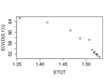
Figure 3: The ETOT and $E(D(\gamma))$ for $m=22,k=20,\alpha=2,\lambda_{1}=0.5,\lambda_{2}=1$

6.2 Data Analysis

In this section we perform the analysis of a real data set to illustrate how the propose methods can be used in practice. We have used the following data set originally obtained from Proschan [19] and here the data indicate the failure times (in hour) of air-conditioning system of two airplanes. The data are provided below.

Plane 7914: 3, 5, 5, 13, 14, 15, 22, 22, 23, 30, 36, 39, 44, 46, 50, 72, 79, 88, 97, 102, 139, 188, 197, 210.
Plane 7913: 1, 4, 11, 16, 18,18, 24, 31, 39, 46, 51, 54, 63, 68, 77, 80, 82, 97, 106, 141, 163, 191, 206, 216.

From the above data sets we have generated two different jointly progressively censored samples with the censoring schemes Scheme 1: $k$ = 20 and $R=(14,0_{(8)})$ and Scheme 2: $k=10$, $R=(2_{(7)},0_{(2)})$. The generated data sets are provided below.

Scheme 1:

$${\bf w}=(1,4,5,13,15,16,22,36,80,97)\ \ \ \ {\bf z}=(0,0,1,1,1,0,1,1,0,0);$$

For the above data set the MLEs, AMLEs, and the two different 90% confidence intervals are provided in Tables 10 and 11. In Figure 4 we have provided the profile log-likelihood function $P(\alpha)$ of the shape parameter $\alpha$ and it is clear that $P(\alpha)$ attains a unique maximum. To get an idea about the joint confidence region of $\alpha$, $\lambda_{1}$, $\lambda_{2}$, we have provided the confidence set of $(\lambda_{1},\lambda_{2})$ for different values of $\alpha$ in Figure 5.

Table 10: real data analysis(scheme-1)

Parameter	MLE	AMLE
$\alpha$	0.983459	0.982218
$\lambda_{1}$	0.017541	0.017622
$\lambda_{2}$	0.017541	0.017622

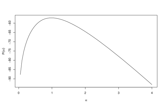
Figure 4: profile-loglikelihood function of shape parameter $\alpha$ for scheme-1

Table 11: real data analysis (90% CI)(scheme-1)

Parameter	90% Asymptotic CI		90% Bootstrap CI
	LL	UL	LL	UL
$\alpha$	0.6508	1.3160	0.7253	1.5900
$\lambda_{1}$	0	0.0426	0.001641	0.05592
$\lambda_{2}$	0	0.0426	0.001644	0.05623

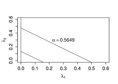
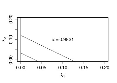
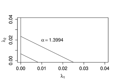
Figure 5: Confidence region of $\lambda_{1}$ and $\lambda_{2}$ for different values $\alpha$ for scheme-1

Scheme 2:

$${\bf w}=(1,3,4,5,5,13,14,31,44,51),{\bf z}=(0,1,0,1,1,1,1,0,1,0);$$

In this case the estimates and the associated confidence intervals are reported in Tables 12 and 13. The profile log-likelihood function $P(\alpha)$ has been provided in Figure 6 and it indicates that it attains a unique maximum. The confidence set of $(\lambda_{1},\lambda_{2})$ for different values of $\alpha$ is provided in Figure 7.

Table 12: real data analysis(scheme-2)

Parameter	MLE	AMLE
$\alpha$	1.1740	1.1612
$\lambda_{1}$	0.01367	0.01421
$\lambda_{2}$	0.009116	0.009479

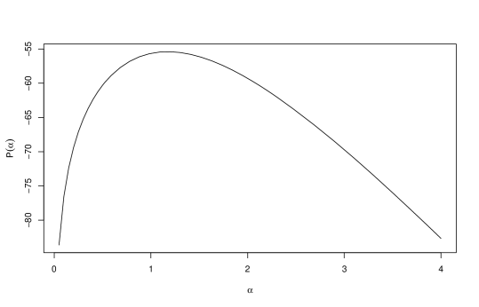
Figure 6: profile-loglikelihood function of shape parameter $\alpha$ for scheme-2

Table 13: real data analysis (90% CI)(scheme-2)

Parameter	90% Asymptotic CI		90% Bootstrap CI
	LL	UL	LL	UL
$\alpha$	0.7533	1.5947	0.91046	2.036402
$\lambda_{1}$	0	0.03351	0.001241	0.03696
$\lambda_{2}$	0	0.02303	0.0007122	0.02532

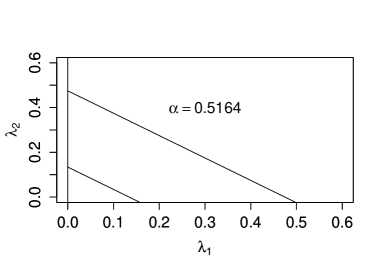
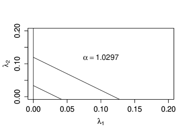
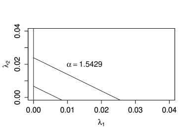
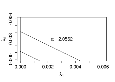
Figure 7: Confidence region of $\lambda_{1}$ and $\lambda_{2}$ for different values of $\alpha$ for Scheme-2

7 Conclusion

In this paper we analyze the new joint progressive censoring (BJPC) for two populations. It is assumed that the lifetimes of the two populations follow Weibull distribution with the same shape parameter but different scale parameters. We obtained the MLEs of the unknown parameters and since they cannot be obtained in explicit forms we have proposed to use AMLEs which can be obtained explicitly. Based on extensive simulation experiments it is observed that the performances of MLEs and AMLEs are very similar in nature. We obtained asymptotic and bootstrap confidence intervals and it is observed that the asymptotic confidence intervals perform quite well even for small sample sizes. We further construct an exact joint confidence set of the unknown parameters and based on the expected volume of the joint confidence set we have proposed an objective function and it has been used to obtain optimum censoring scheme. Note that all the developments in this paper are mainly based on the classical approach. It will be important to develop the necessary Bayesian inference. It may be mentioned that in this paper we have considered the sample sizes to be equal from both the populations, although most of the results can be extended even when they are not equal.

Appendix

proof of Lemma 1:

$P(\alpha)\rightarrow-\infty\hskip 14.22636pt\mbox{as}\hskip 14.22636pt\alpha\rightarrow 0$

$$\lim_{\alpha\to\infty}P(\alpha) = -k\lim{\alpha\to\infty}\frac{(\sum_{i=1}^{k-1}(R_{i}+1)\ln(w_{i}){w_{i}}^{\alpha}+(m-\sum_{i=1}^{k-1}(R_{i}+1))\ln(w_{i}){w_{k}}^{\alpha}))}{(\sum_{i=1}^{k-1}(R_{i}+1){w_{i}}^{\alpha}+(m-\sum_{i=1}^{k-1}(R_{i}+1)){w_{k}}^{\alpha}))}+\sum_{i=1}^{k}\ln(w_{i})$$

$$= -k\ln(w_{k})+\sum_{i=1}^{k}\ln(w_{i})$$

$$= \sum_{i=1}^{k}\ln(\frac{w_{i}}{w_{k}})<0$$

$\Rightarrow P(\alpha)\rightarrow-\infty\hskip 14.22636ptas\hskip 14.22636pt\alpha\rightarrow\infty$ This concludes mle ${\alpha}^{*}$ is attained in $(0,\infty)$.

According to Balakrishnan and Kateri [6] $H(\alpha)$ is increasing function of $\alpha$ and $\frac{1}{\alpha}$ is decreasing in $\alpha$ resulting unique solution of equation of equation$(5)$.

proof of Lemma 2: The proof can be obtained similarly as the proof of Lemma 2 of Mondal and Kundu [13] using $m=n$.

References

- [1] Ashour, S. and Eraki, O. (2014), “Parameter estimation for multiple Weibull populations under joint type-II censoring”, International Journal of Advanced Statistics and Probability, vol 2, 2, pp 102–107.
- [2] Balakrishnan, N. and Aggarwala, R. (2000), Progressive censoring: theory, methods, and applications, Birkhauser, Boston, U.S.A.
- [3] Balakrishnan, N. and Cramer, E. (2014), The art of progressive censoring, Springer, New York.
- [4] Balakrishnan, N. and Kannan, N. and Lin, C. T. and Ng, H. K. T. (2003), “Point and interval estimation for Gaussian distribution, based on progressively Type-II censored samples”, IEEE Transactions on Reliability, vol 52, 1, pp 90–95.
- [5] Balakrishnan, N. and Kannan, N. and Lin, C. T. and Wu, S. J. S. (2004), “Inference for the extreme value distribution under progressive Type-II censoring”, Journal of Statistical Computation and Simulation, vol 74, 1, pp 25–45.
- [6] Balakrishnan, N. and Kateri, M. (2008), “On the maximum likelihood estimation of parameters of Weibull distribution based on complete and censored data”, Statistics & Probability Letters, vol 78, 17, pp 2971–2975.
- [7] Balakrishnan, N. and Rasouli, A. (2008), “Exact likelihood inference for two exponential populations under joint Type-II censoring”, Computational Statistics & Data Analysis, vol 52, 5, pp 2725–2738,
- [8] Balakrishnan, N. and Su, F. and Liu, K. Y. (2015), “Exact likelihood inference for exponential populations under joint progressive Type-II censoring”, Communications in Statistics-Simulation and Computation, vol 44, 4, pp 902–923.
- [9] Balakrishnan, N. and Varadan, J. (1991), “Approximate MLEs for the location and scale parameters of the extreme value distribution with censoring”, IEEE Transactions on Reliability, vol 40, 2,pp 146–151.
- [10] Burkschat, M. and Cramer, E. and Kamps, U. (2006), “On optimal schemes in progressive censoring”, Statistics & probability letters, vol 76, 10, pp 1032–1036.
- [11] Burkschat, M. and Cramer, E. and Kamps, U. (2007), “Optimality criteria and optimal schemes in progressive censoring”, Communications in Statistics—Theory and Methods, vol 36, 7, pp 1419–1431.
- [12] Doostparast, M. and Ahmadi, M. V. and Ahmadi, J. (2013), “Bayes Estimation Based on Joint Progressive Type II Censored Data Under LINEX Loss Function”, Communications in Statistics-Simulation and Computation, vol 42, 8,pp 1865–1886.
- [13] Mondal, S. and Kundu, D. (2016), “A new two sample Type-II progressive censoring scheme”, arXiv:1609.05805.
- [14] Ng, H. K. T. and Chan, P. S. and Balakrishnan, N. (2004), “Optimal progressive censoring plans for the Weibull distribution”, Technometrics, vol 46, 4, pp 470–481.
- [15] Pareek, B. and Kundu, D. and Kumar, S. (2009), “On progressively censored competing risks data for Weibull distributions”,Computational Statistics & Data Analysis, vol 53, 12, pp 4083–4094.
- [16] Parsi, S. and Ganjali, M. and Farsipour, N. S. (2011), “Conditional maximum likelihood and interval estimation for two Weibull populations under joint Type-II progressive censoring”, Communications in Statistics-Theory and Methods, vol 40, 12, pp 2117–2135.
- [17] Pradhan, B. and Kundu, D. (2009), “On progressively censored generalized exponential distribution” , Test, vol 18, 3, pp 497–515.
- [18] Pradhan, B. and Kundu, D. (2013), “Inference and optimal censoring schemes for progressively censored Birnbaum–Saunders distribution”, Journal of Statistical Planning and Inference, vol 143, 6, pp 1098–1108,
- [19] Proschan, F. (1963), “Theoretical explanation of observed decreasing failure rate”, Technometrics, vol 15, 375 - 383.
- [20] Rasouli, A. and Balakrishnan, N. (2010), “Exact likelihood inference for two exponential populations under joint progressive type-II censoring”, Communications in Statistics—Theory and Methods, vol 39, 12, pp 2172–2191.
- [21] Srivastava, J.N. (1987), “More efficient and less time consuming censoring design for life testing”, Journal of Statistical Planning and Inference, vol. 16, 389 - 413.
- [22] Wang, B. X. and Yu, K. and Jones, M. C. (2010), “Inference under progressively type II right-censored sampling for certain lifetime distributions”, Technometrics, vol 52, 4, pp 453–460.
- [23] Wu, S. J. (2002), “Estimations of the parameters of the Weibull distribution with progressively censored data”, Journal of the Japan Statistical Society, vol 32, 2, pp 155–163.