Butterfly Counting in Bipartite Networks

Abstract

We consider the problem of counting motifs in bipartite affiliation networks, such as author-paper, user-product, and actor-movie relations. We focus on counting the number of occurrences of a “butterfly”, a complete $2\times 2$ biclique, the simplest cohesive higher-order structure in a bipartite graph. Our main contribution is a suite of randomized algorithms that can quickly approximate the number of butterflies in a graph with a provable guarantee on accuracy. An experimental evaluation on large real-world networks shows that our algorithms return accurate estimates within a few seconds, even for networks with trillions of butterflies and hundreds of millions of edges.

1 Introduction

Graph motifs are used to model and examine interactions among small sets of vertices in networks. Finding frequent patterns of interactions can reveal functions of participating entities Seshadhri et al. (2014); Jha et al. (2015); Pinar et al. (2017); Ahmed et al. (2016); Bressan et al. (2017); Jain and Seshadhri (2017) and help characterize the network. Also known as graphlets or higher-order structures, motifs are regarded as basic building blocks of complex networks in domains such as social networks, food webs, and neural networks Milo et al. (2002). For this reason, finding and counting motifs are among the most important and widely used network analysis procedures. The triangle is the most basic motif in a unipartite network, and graph mining literature is abundant with triangle counting algorithms for stationary networks Seshadhri et al. (2014); Tsourakakis et al. (2009) as well as dynamic networks Lim and Kang (2015); De Stefani et al. (2016); Pavan et al. (2013). There are also studies that consider structures with more than 3 vertices Jha et al. (2015); Pinar et al. (2017); Jain and Seshadhri (2017), but these primarily focus on cliques, such as 4-cliques and 5-cliques.

In this work, we focus on bipartite (affiliation) networks, an important type of network for many applications Borgatti and Everett (1997); Latapy et al. (2008). For example, relationships between authors and papers can be modeled as a bipartite graph, where authors form one vertex partition, papers form the other vertex partition, and an author has an edge to each paper that she published. Other examples include user-product relations, word-document affiliations, and actor-movie networks. Bipartite graphs can represent hypergraphs that capture many-to-many relations among entities. A hypergraph $H=(V_{H},E_{H})$ with vertex set $V_{H}$ and edge set $E_{H}$, where each hyper-edge $h\in E_{H}$ is a set of vertices, can be represented as a bipartite graph with vertex set $V_{H}\cup E_{H}$ with one partition for $V_{H}$ and another for $E_{H}$, and an edge from a vertex $v\in V_{H}$ to an edge $h\in E_{H}$ if $v$ is a part of $h$ in $H$. For example, a hypergraph corresponding to an author-paper relation where each paper is associated with a set of authors can be represented using a bipartite graph with one partition for authors and one for papers.

A common approach to handle a bipartite network is to reduce it to a unipartite co-occurrence network by a projection Newman (2001b, a). A projection selects a vertex partition as the set of entities, and creates a unipartite network whose vertex set is the set of all entities and where two entities are connected if they share an affiliation in the bipartite network. For the author-paper network, a projection on the authors creates a unipartite co-authorship network. However, such a projection causes the number of edges in the graph to explode, artificially boosts the number of triangles and clustering coefficients, and results in information loss. For instance, we observed up to 4 orders of magnitude increase in size when the bipartite network between wikipedia articles and their editors in French is projected onto a unipartite network of articles – number of edges goes from $22$M to more than $200$B. As a result, it is preferable to analyze bipartite networks directly.

While there is extensive work on motif counting in unipartite networks, these do not apply to bipartite networks. Motifs in bipartite networks are very different from motifs in a unipartite network. The most commonly studied motifs in a unipartite network are cliques of small sizes, but a bipartite graph does not have any cliques with more than two vertices, not even a triangle! Instead, natural motifs in a bipartite network are bicliques of small size.

The most basic motif that models cohesion in a bipartite network is the complete $2\times 2$ biclique, also known as a butterfly Aksoy et al. (2017); Sarıyüce and Pinar (2018) or a rectangle Wang et al. (2014). Although there have been attempts at defining other cohesive motifs in bipartite networks, such as the complete $3\times 3$ biclique Borgatti and Everett (1997) and $4$-path Opsahl (2013), the butterfly remains the smallest unit of cohesion, and has been used in defining basic metrics such as the clustering coefficient in a bipartite graph Robins and Alexander (2004); Lind et al. (2005). In particular, it is the smallest subgraph that has multiple vertices on each side with multiple common neighbors. It can be considered as playing the same role in bipartite networks as the triangle did in unipartite networks – a building block for community structure. We aim to derive methods which can accurately estimate the number of butterflies in a given large bipartite graph. We view butterfly counting as a first, but important step towards general methods for motif counting and analysis of bipartite affiliation networks.

Contributions: We present fast algorithms to accurately estimate the number of butterflies in a bipartite network. Our algorithms are simple to implement, backed up by theoretical guarantees, and have good practical performance.

• Exact Butterfly Counting: We first present an efficient exact algorithm, ExactBFC, for counting the number of butterflies in a network. We use a simple measure, the sum of the squares of vertex degrees, to choose which vertex partition of the bipartite graph to start the algorithm from. Leveraging the imbalance between vertex partitions yields significant speedups over the state-of-the-art Wang et al. (2014).

• Randomized Approximate Butterfly Counting: We introduce the first randomized algorithms to find the approximate number of butterflies in a network by sampling. Our algorithms are able to derive accurate estimates with error as low as $1$% within a few seconds, are much faster than the exact algorithms, and have an insignificant memory print. We present two types of randomized algorithms.

  • One-shot Sparsification techniques assume that the entire graph is available for processing. They thin-down the graph to a much smaller sparsified graph through choosing each edge of the original graph with a certain randomized procedure. Exact butterfly counting is then applied on the sparsified graph to estimate the number of butterflies in the original graph. We present two such algorithms – ESpar  and ClrSpar.

  • Local Sampling algorithms, on the other hand, can work under limited access to the input graph. They randomly sample small subgraphs local to an element of the graph, and use them to compute an estimate. This is in contrast to sparsification, which needs a global view of the graph. We investigate sampling of subgraphs localized around a vertex (VSamp), edge (ESamp), and a wedge (WSamp). Sampling algorithms are especially useful when there is a rate-limited API that provides random samples, such as the GNIP framework for Twitter gni (2017) and the Graph API of Facebook fbg (2017). In the rest of this paper, when we say “sampling algorithms”, we mean local sampling algorithms.

• Provable Guarantees: We prove that the randomized algorithms yield estimates that are equal to the actual number of butterflies in the graph, in expectation. Through a careful analysis of their variance, we show that it is possible to reduce the estimation error to any desired level, through independent repetitions (sampling) or through an appropriate choice of parameters (sparsification).

• Experiments on real-world networks: We present results of an evaluation of our algorithms on large real-world networks. These results show that the algorithms can handle massive graphs with hundreds of millions of edges and trillions of butterflies. Our most efficient sampling algorithm, which we call ESamp+Fast-eBFC, gives estimates with a relative error less than $1$ percent within $5$ seconds, even for large graphs with trillions of butterflies. On such large graphs, (exact) algorithms from prior work took tens of thousands of seconds. We observed a similar behavior with our best one-shot sparsification algorithm, ESpar, which typically yields estimates with error less than $1$ percent, within $4$ secs.

2 Preliminaries

We consider simple, unweighted, bipartite graphs, where there are no self-loops or multiple edges between vertices. Let $G=(V,E)$ be a simple bipartite graph with $n=|V|$ vertices and $m=|E|$ edges. Vertex set $V$ is partitioned into two sets $L$ and $R$ such that $V=L\cup R$ and $L\cap R=\emptyset$. The edge set $E\subseteq L\times R$. For $v\in V$, $\Gamma_{v}=\{u|(v,u)\in E\}$ denotes the set of vertices adjacent to $v$ (neighbors) and $d_{v}=|\Gamma_{v}|$ is the degree of $v$. $\Delta$ denotes the maximum degree of a vertex in the graph. In addition, $\Gamma^{2}_{v}=\{w|(w,u)\in E\land w\neq v,\leavevmode\nobreak\ \forall\leavevmode\nobreak\ u\in\Gamma_{v}\}$ is the set of vertices that are exactly in distance 2 from $v$, i.e., neighbors of the neighbors of $v$ (excluding $v$ itself). A wedge in $G$ is a path of length two.

A biclique is a complete bipartite subgraph, and is parameterized by the number of vertices in each partition; for integers $\alpha,\beta$, an $\alpha\times\beta$ biclique in a bipartite graph is a complete subgraph with $\alpha$ vertices in $L$ and $\beta$ vertices in $R$. A butterfly in $G$ is a $2\times 2$ biclique and consists of four vertices $\{a,b,x,y\}\subset V$ where $a,b\in L$ and $x,y\in R$ such that edges $(a,x)$, $(a,y)$, $(b,x)$, and $(b,y)$ all exist in $E$. Let $\mathbin{\mathchoice{\vbox{\hbox{\hskip 1.29167pt\begin{picture}(1.0,1.0)\roundcap\put(0.0,0.27){\line(1,0){1.0}} \put(1.0,0.27){\line(-1,1){1.0}} \put(0.0,1.27){\line(1,0){1.0}} \put(0.0,0.27){\line(1,1){1.0}} \end{picture}\hskip 1.29167pt\vspace{-0.6ex} }}}{\vbox{\hbox{\hskip 1.29167pt\begin{picture}(1.0,1.0)\roundcap\put(0.0,0.27){\line(1,0){1.0}} \put(1.0,0.27){\line(-1,1){1.0}} \put(0.0,1.27){\line(1,0){1.0}} \put(0.0,0.27){\line(1,1){1.0}} \end{picture}\hskip 1.29167pt\vspace{-0.6ex} }}}{\vbox{\hbox{\hskip 1.29167pt\begin{picture}(1.0,1.0)\roundcap\put(0.0,0.27){\line(1,0){1.0}} \put(1.0,0.27){\line(-1,1){1.0}} \put(0.0,1.27){\line(1,0){1.0}} \put(0.0,0.27){\line(1,1){1.0}} \end{picture}\hskip 1.29167pt\vspace{-0.6ex} }}}{\vbox{\hbox{\hskip 1.29167pt\begin{picture}(1.0,1.0)\roundcap\put(0.0,0.27){\line(1,0){1.0}} \put(1.0,0.27){\line(-1,1){1.0}} \put(0.0,1.27){\line(1,0){1.0}} \put(0.0,0.27){\line(1,1){1.0}} \end{picture}\hskip 1.29167pt\vspace{-0.6ex} }}}}(G)$ denote the number of butterflies in $G$ (we use notation $\mathbin{\mathchoice{\vbox{\hbox{\hskip 1.29167pt\begin{picture}(1.0,1.0)\roundcap\put(0.0,0.27){\line(1,0){1.0}} \put(1.0,0.27){\line(-1,1){1.0}} \put(0.0,1.27){\line(1,0){1.0}} \put(0.0,0.27){\line(1,1){1.0}} \end{picture}\hskip 1.29167pt\vspace{-0.6ex} }}}{\vbox{\hbox{\hskip 1.29167pt\begin{picture}(1.0,1.0)\roundcap\put(0.0,0.27){\line(1,0){1.0}} \put(1.0,0.27){\line(-1,1){1.0}} \put(0.0,1.27){\line(1,0){1.0}} \put(0.0,0.27){\line(1,1){1.0}} \end{picture}\hskip 1.29167pt\vspace{-0.6ex} }}}{\vbox{\hbox{\hskip 1.29167pt\begin{picture}(1.0,1.0)\roundcap\put(0.0,0.27){\line(1,0){1.0}} \put(1.0,0.27){\line(-1,1){1.0}} \put(0.0,1.27){\line(1,0){1.0}} \put(0.0,0.27){\line(1,1){1.0}} \end{picture}\hskip 1.29167pt\vspace{-0.6ex} }}}{\vbox{\hbox{\hskip 1.29167pt\begin{picture}(1.0,1.0)\roundcap\put(0.0,0.27){\line(1,0){1.0}} \put(1.0,0.27){\line(-1,1){1.0}} \put(0.0,1.27){\line(1,0){1.0}} \put(0.0,0.27){\line(1,1){1.0}} \end{picture}\hskip 1.29167pt\vspace{-0.6ex} }}}}$ when $G$ is clear from the context). For vertex $v\in V$, let $\mathbin{\mathchoice{\vbox{\hbox{\hskip 1.29167pt\begin{picture}(1.0,1.0)\roundcap\put(0.0,0.27){\line(1,0){1.0}} \put(1.0,0.27){\line(-1,1){1.0}} \put(0.0,1.27){\line(1,0){1.0}} \put(0.0,0.27){\line(1,1){1.0}} \end{picture}\hskip 1.29167pt\vspace{-0.6ex} }}}{\vbox{\hbox{\hskip 1.29167pt\begin{picture}(1.0,1.0)\roundcap\put(0.0,0.27){\line(1,0){1.0}} \put(1.0,0.27){\line(-1,1){1.0}} \put(0.0,1.27){\line(1,0){1.0}} \put(0.0,0.27){\line(1,1){1.0}} \end{picture}\hskip 1.29167pt\vspace{-0.6ex} }}}{\vbox{\hbox{\hskip 1.29167pt\begin{picture}(1.0,1.0)\roundcap\put(0.0,0.27){\line(1,0){1.0}} \put(1.0,0.27){\line(-1,1){1.0}} \put(0.0,1.27){\line(1,0){1.0}} \put(0.0,0.27){\line(1,1){1.0}} \end{picture}\hskip 1.29167pt\vspace{-0.6ex} }}}{\vbox{\hbox{\hskip 1.29167pt\begin{picture}(1.0,1.0)\roundcap\put(0.0,0.27){\line(1,0){1.0}} \put(1.0,0.27){\line(-1,1){1.0}} \put(0.0,1.27){\line(1,0){1.0}} \put(0.0,0.27){\line(1,1){1.0}} \end{picture}\hskip 1.29167pt\vspace{-0.6ex} }}}}_{v}$ denote the number of butterflies that contain $v$. Similarly, for edge $e\in E$, let $\mathbin{\mathchoice{\vbox{\hbox{\hskip 1.29167pt\begin{picture}(1.0,1.0)\roundcap\put(0.0,0.27){\line(1,0){1.0}} \put(1.0,0.27){\line(-1,1){1.0}} \put(0.0,1.27){\line(1,0){1.0}} \put(0.0,0.27){\line(1,1){1.0}} \end{picture}\hskip 1.29167pt\vspace{-0.6ex} }}}{\vbox{\hbox{\hskip 1.29167pt\begin{picture}(1.0,1.0)\roundcap\put(0.0,0.27){\line(1,0){1.0}} \put(1.0,0.27){\line(-1,1){1.0}} \put(0.0,1.27){\line(1,0){1.0}} \put(0.0,0.27){\line(1,1){1.0}} \end{picture}\hskip 1.29167pt\vspace{-0.6ex} }}}{\vbox{\hbox{\hskip 1.29167pt\begin{picture}(1.0,1.0)\roundcap\put(0.0,0.27){\line(1,0){1.0}} \put(1.0,0.27){\line(-1,1){1.0}} \put(0.0,1.27){\line(1,0){1.0}} \put(0.0,0.27){\line(1,1){1.0}} \end{picture}\hskip 1.29167pt\vspace{-0.6ex} }}}{\vbox{\hbox{\hskip 1.29167pt\begin{picture}(1.0,1.0)\roundcap\put(0.0,0.27){\line(1,0){1.0}} \put(1.0,0.27){\line(-1,1){1.0}} \put(0.0,1.27){\line(1,0){1.0}} \put(0.0,0.27){\line(1,1){1.0}} \end{picture}\hskip 1.29167pt\vspace{-0.6ex} }}}}_{e}$ denote the number of butterflies containing $e$ (See Figure 1). Our goal is to compute $\mathbin{\mathchoice{\vbox{\hbox{\hskip 1.29167pt\begin{picture}(1.0,1.0)\roundcap\put(0.0,0.27){\line(1,0){1.0}} \put(1.0,0.27){\line(-1,1){1.0}} \put(0.0,1.27){\line(1,0){1.0}} \put(0.0,0.27){\line(1,1){1.0}} \end{picture}\hskip 1.29167pt\vspace{-0.6ex} }}}{\vbox{\hbox{\hskip 1.29167pt\begin{picture}(1.0,1.0)\roundcap\put(0.0,0.27){\line(1,0){1.0}} \put(1.0,0.27){\line(-1,1){1.0}} \put(0.0,1.27){\line(1,0){1.0}} \put(0.0,0.27){\line(1,1){1.0}} \end{picture}\hskip 1.29167pt\vspace{-0.6ex} }}}{\vbox{\hbox{\hskip 1.29167pt\begin{picture}(1.0,1.0)\roundcap\put(0.0,0.27){\line(1,0){1.0}} \put(1.0,0.27){\line(-1,1){1.0}} \put(0.0,1.27){\line(1,0){1.0}} \put(0.0,0.27){\line(1,1){1.0}} \end{picture}\hskip 1.29167pt\vspace{-0.6ex} }}}{\vbox{\hbox{\hskip 1.29167pt\begin{picture}(1.0,1.0)\roundcap\put(0.0,0.27){\line(1,0){1.0}} \put(1.0,0.27){\line(-1,1){1.0}} \put(0.0,1.27){\line(1,0){1.0}} \put(0.0,0.27){\line(1,1){1.0}} \end{picture}\hskip 1.29167pt\vspace{-0.6ex} }}}}(G)$ for a graph $G$. We summarize our notation in Table 1.

When estimating the number of butterflies, we look for provable guarantees on the estimates computed using the following notion of randomized approximation. For parameters $\epsilon,\delta\in[0,1]$, an $(\epsilon,\delta)-{}$approximation of a number $Z$ is a random variable $\hat{Z}$ such that $\Pr[|\hat{Z}-Z|>\epsilon Z]\leq\delta$.

Figure 1: There are 4 butterflies in the entire graph, and the number of per-vertex and per-edge butterflies are shown for some vertices/edges.

$G=(V,E)$	simple bipartite graph with vertices $V$ and edges $E$
$V=L\cup R$	vertex partitions $L$ and $R$
$\Gamma_{v}$	set of vertices adjacent to $v$, i.e., $\{u|(v,u)\in E\}$
$d_{v}$	degree of vertex $v$, i.e., $|\Gamma_{v}|$
$n,m,\land$	number of vertices ($|V|$), edges ($|E|$), and wedges ($\sum_{v\in V}{{d_{v}\choose{2}}}$)
$\Delta$	maximum degree of a vertex in the graph
$\Gamma^{2}_{v}$	distance-2 neighbors of $v$ (excluding itself)
$\mathbin{\mathchoice{\vbox{\hbox{\hskip 1.29167pt\begin{picture}(1.0,1.0)\roundcap\put(0.0,0.27){\line(1,0){1.0}} \put(1.0,0.27){\line(-1,1){1.0}} \put(0.0,1.27){\line(1,0){1.0}} \put(0.0,0.27){\line(1,1){1.0}} \end{picture}\hskip 1.29167pt\vspace{-0.6ex} }}}{\vbox{\hbox{\hskip 1.29167pt\begin{picture}(1.0,1.0)\roundcap\put(0.0,0.27){\line(1,0){1.0}} \put(1.0,0.27){\line(-1,1){1.0}} \put(0.0,1.27){\line(1,0){1.0}} \put(0.0,0.27){\line(1,1){1.0}} \end{picture}\hskip 1.29167pt\vspace{-0.6ex} }}}{\vbox{\hbox{\hskip 1.29167pt\begin{picture}(1.0,1.0)\roundcap\put(0.0,0.27){\line(1,0){1.0}} \put(1.0,0.27){\line(-1,1){1.0}} \put(0.0,1.27){\line(1,0){1.0}} \put(0.0,0.27){\line(1,1){1.0}} \end{picture}\hskip 1.29167pt\vspace{-0.6ex} }}}{\vbox{\hbox{\hskip 1.29167pt\begin{picture}(1.0,1.0)\roundcap\put(0.0,0.27){\line(1,0){1.0}} \put(1.0,0.27){\line(-1,1){1.0}} \put(0.0,1.27){\line(1,0){1.0}} \put(0.0,0.27){\line(1,1){1.0}} \end{picture}\hskip 1.29167pt\vspace{-0.6ex} }}}}(G)$ (or $\mathbin{\mathchoice{\vbox{\hbox{\hskip 1.29167pt\begin{picture}(1.0,1.0)\roundcap\put(0.0,0.27){\line(1,0){1.0}} \put(1.0,0.27){\line(-1,1){1.0}} \put(0.0,1.27){\line(1,0){1.0}} \put(0.0,0.27){\line(1,1){1.0}} \end{picture}\hskip 1.29167pt\vspace{-0.6ex} }}}{\vbox{\hbox{\hskip 1.29167pt\begin{picture}(1.0,1.0)\roundcap\put(0.0,0.27){\line(1,0){1.0}} \put(1.0,0.27){\line(-1,1){1.0}} \put(0.0,1.27){\line(1,0){1.0}} \put(0.0,0.27){\line(1,1){1.0}} \end{picture}\hskip 1.29167pt\vspace{-0.6ex} }}}{\vbox{\hbox{\hskip 1.29167pt\begin{picture}(1.0,1.0)\roundcap\put(0.0,0.27){\line(1,0){1.0}} \put(1.0,0.27){\line(-1,1){1.0}} \put(0.0,1.27){\line(1,0){1.0}} \put(0.0,0.27){\line(1,1){1.0}} \end{picture}\hskip 1.29167pt\vspace{-0.6ex} }}}{\vbox{\hbox{\hskip 1.29167pt\begin{picture}(1.0,1.0)\roundcap\put(0.0,0.27){\line(1,0){1.0}} \put(1.0,0.27){\line(-1,1){1.0}} \put(0.0,1.27){\line(1,0){1.0}} \put(0.0,0.27){\line(1,1){1.0}} \end{picture}\hskip 1.29167pt\vspace{-0.6ex} }}}}$)	number of butterflies in graph $G$
$\mathbin{\mathchoice{\vbox{\hbox{\hskip 1.29167pt\begin{picture}(1.0,1.0)\roundcap\put(0.0,0.27){\line(1,0){1.0}} \put(1.0,0.27){\line(-1,1){1.0}} \put(0.0,1.27){\line(1,0){1.0}} \put(0.0,0.27){\line(1,1){1.0}} \end{picture}\hskip 1.29167pt\vspace{-0.6ex} }}}{\vbox{\hbox{\hskip 1.29167pt\begin{picture}(1.0,1.0)\roundcap\put(0.0,0.27){\line(1,0){1.0}} \put(1.0,0.27){\line(-1,1){1.0}} \put(0.0,1.27){\line(1,0){1.0}} \put(0.0,0.27){\line(1,1){1.0}} \end{picture}\hskip 1.29167pt\vspace{-0.6ex} }}}{\vbox{\hbox{\hskip 1.29167pt\begin{picture}(1.0,1.0)\roundcap\put(0.0,0.27){\line(1,0){1.0}} \put(1.0,0.27){\line(-1,1){1.0}} \put(0.0,1.27){\line(1,0){1.0}} \put(0.0,0.27){\line(1,1){1.0}} \end{picture}\hskip 1.29167pt\vspace{-0.6ex} }}}{\vbox{\hbox{\hskip 1.29167pt\begin{picture}(1.0,1.0)\roundcap\put(0.0,0.27){\line(1,0){1.0}} \put(1.0,0.27){\line(-1,1){1.0}} \put(0.0,1.27){\line(1,0){1.0}} \put(0.0,0.27){\line(1,1){1.0}} \end{picture}\hskip 1.29167pt\vspace{-0.6ex} }}}}_{v(e)}$	number of butterflies that contain vertex $v$ (edge $e$)

Table 1: Notations

Networks and Experimental Setup.

Since we frequently present evaluation results close to the algorithm descriptions, we give some details about the data used for evaluation. We used massive real-world bipartite networks, selected from the publicly available KONECT network repository . The graphs that we have used are summarized in Table 2. We converted all graphs to simple, undirected graphs by removing edge directions (if graph was directed), and by removing all self-loops, multiple edges, and vertices with degree zero. We implemented all algorithms in C++, compiled with Visual C++ 2015 compiler (Version 14.0), and report the runtimes on a machine equipped with a $3.50$ GHz Intel(R) Xeon(R) CPU E3-1241 v3 and $16.0$ GB memory.

Bipartite graph	$|L|$	$|R|$	$|E|$	$\sum_{\ell\in{}L}{d_{\ell}^{2}}$	$\sum_{r\in{}R}{d_{r}^{2}}$	$\mathbin{\mathchoice{\vbox{\hbox{\hskip 1.29167pt\begin{picture}(1.0,1.0)\roundcap\put(0.0,0.27){\line(1,0){1.0}} \put(1.0,0.27){\line(-1,1){1.0}} \put(0.0,1.27){\line(1,0){1.0}} \put(0.0,0.27){\line(1,1){1.0}} \end{picture}\hskip 1.29167pt\vspace{-0.6ex} }}}{\vbox{\hbox{\hskip 1.29167pt\begin{picture}(1.0,1.0)\roundcap\put(0.0,0.27){\line(1,0){1.0}} \put(1.0,0.27){\line(-1,1){1.0}} \put(0.0,1.27){\line(1,0){1.0}} \put(0.0,0.27){\line(1,1){1.0}} \end{picture}\hskip 1.29167pt\vspace{-0.6ex} }}}{\vbox{\hbox{\hskip 1.29167pt\begin{picture}(1.0,1.0)\roundcap\put(0.0,0.27){\line(1,0){1.0}} \put(1.0,0.27){\line(-1,1){1.0}} \put(0.0,1.27){\line(1,0){1.0}} \put(0.0,0.27){\line(1,1){1.0}} \end{picture}\hskip 1.29167pt\vspace{-0.6ex} }}}{\vbox{\hbox{\hskip 1.29167pt\begin{picture}(1.0,1.0)\roundcap\put(0.0,0.27){\line(1,0){1.0}} \put(1.0,0.27){\line(-1,1){1.0}} \put(0.0,1.27){\line(1,0){1.0}} \put(0.0,0.27){\line(1,1){1.0}} \end{picture}\hskip 1.29167pt\vspace{-0.6ex} }}}}$
$\left(10^{4},10\right)$-biclique	10000	10	100000	1000000	1000000000	2249775000
DBPedia-Location	172079	53407	293697	629983	245744643	3761594
Wikipedia (fr)	288275	3992426	22090703	2186560482259	795544489	601291038864
Twitter	175214	530418	1890661	74184693	1943171143	206508691
Amazon	2146057	1230915	5743258	828704126	437163474	35849304
Journal	3201203	7489073	112307385	9565595799	5398290985343	3297158439527
Wiki-en	3819691	21416395	122075170	12576726351444	23256846234	2036443879822
Deli	833081	33778221	101798957	85945241607	52787267117	56892252403
Orkut	2783196	8730857	327037487	156580049011	4900153043329	22131701213295
Web	27665730	12756244	140613762	1733678094524	211149951033914	20067567209850

Table 2: Bipartite network datasets. $L$ and $R$ are vertex partitions, $E$ is the edge set. The sum of degree squares for $L$ and $R$, and the number of butterflies are shown.

3 Related Work

Bipartite graph motifs: Modeling the smallest unit of cohesion enables a principled way to analyze networks. While the literature is quite rich with the studies on counting triangles and small cliques in unipartite graphs Seshadhri et al. (2014); Jha et al. (2015); Pinar et al. (2017); Ahmed et al. (2016); Pavan et al. (2013); Tangwongsan et al. (2013); Bressan et al. (2017); Jain and Seshadhri (2017), these works are not applicable to bipartite networks. To the best of our knowledge, Borgatti and Everett Borgatti and Everett (1997) are the first to consider cohesive structures in bipartite networks to analyze social networks. They proposed to use the $3\times 3$ biclique as the smallest cohesive structure, motivated by the fact that a triangle in a unipartite graph has three vertices, and the same should be considered for both vertex sets of the bipartite graph. Opsahl also proposed a similar approach to define the clustering coefficient in affiliation networks Opsahl (2013). Robins and Alexander argued that the smallest structure with multiple vertices on both vertex sets is a better model for measuring cohesion in bipartite networks Robins and Alexander (2004), as also discussed in a later work Lind et al. (2005). They used the ratio of the number of $2\times 2$ bicliques (butterflies) to the number of $3$-paths (a path of three edges) to define the clustering coefficient in bipartite graphs. The butterfly is also adopted in a recent work by Aksoy et al. Aksoy et al. (2017) to generate bipartite graphs with community structure. Butterfly counting is also applicable to the study of graphical codes (Halford and Chugg Halford and Chugg (2006)). The numbers of cycles of length $g$, $g+2$, and $g+4$ in bipartite graphs, where $g$ is the girth, characterize the decoding complexity – note that the butterfly is the simplest non-trivial cycle in a bipartite graph.

Random Sampling for Motif Counting: There has been much interest in recent years for counting motifs via random sampling, mostly focused on unipartite graphs and triangles. Works on triangle counting include edge sampling Tsourakakis et al. (2009), subsequently improved by colorful sampling Pagh and Tsourakakis (2012), on vertex and edge sampling Wu et al. (2016); Itai and Rodeh (1978), wedge sampling Seshadhri et al. (2014), a hybrid scheme that considers the edge and wedge sampling Turkoglu and Turk (2017), neighborhood sampling Pavan et al. (2013), and a recent space-efficient algorithm De Stefani et al. (2016) based on reservoir-sampling. To the best of our knowledge, random sampling for butterfly counting in bipartite networks has not been studied in the past.

Butterfly Counting: The closest work to ours is by Wang et al. Wang et al. (2014), who presented exact algorithms for butterfly (rectangle) counting. Their algorithms outperform generic matrix-multiplication based methods for counting cycles in a graph Alon et al. (1997). We present an improved algorithm for exact butterfly counting, and then present more efficient randomized algorithms for approximate butterfly counting.

4 Exact Butterfly Counting

We first present the basic equation for the number of butterflies in a bipartite graph $G$ and the base (state-of-the-art) algorithm by Wang et al. Wang et al. (2014) that implements the equation.

Lemma 1.

For a bipartite graph $G=(V=(L\cup R),E)$,
$(1)\leavevmode\nobreak\ \mathbin{\mathchoice{\vbox{\hbox{\hskip 1.29167pt\begin{picture}(1.0,1.0)\roundcap\put(0.0,0.27){\line(1,0){1.0}} \put(1.0,0.27){\line(-1,1){1.0}} \put(0.0,1.27){\line(1,0){1.0}} \put(0.0,0.27){\line(1,1){1.0}} \end{picture}\hskip 1.29167pt\vspace{-0.6ex} }}}{\vbox{\hbox{\hskip 1.29167pt\begin{picture}(1.0,1.0)\roundcap\put(0.0,0.27){\line(1,0){1.0}} \put(1.0,0.27){\line(-1,1){1.0}} \put(0.0,1.27){\line(1,0){1.0}} \put(0.0,0.27){\line(1,1){1.0}} \end{picture}\hskip 1.29167pt\vspace{-0.6ex} }}}{\vbox{\hbox{\hskip 1.29167pt\begin{picture}(1.0,1.0)\roundcap\put(0.0,0.27){\line(1,0){1.0}} \put(1.0,0.27){\line(-1,1){1.0}} \put(0.0,1.27){\line(1,0){1.0}} \put(0.0,0.27){\line(1,1){1.0}} \end{picture}\hskip 1.29167pt\vspace{-0.6ex} }}}{\vbox{\hbox{\hskip 1.29167pt\begin{picture}(1.0,1.0)\roundcap\put(0.0,0.27){\line(1,0){1.0}} \put(1.0,0.27){\line(-1,1){1.0}} \put(0.0,1.27){\line(1,0){1.0}} \put(0.0,0.27){\line(1,1){1.0}} \end{picture}\hskip 1.29167pt\vspace{-0.6ex} }}}}(G)=\frac{1}{2}\sum_{v\in L}{\mathbin{\mathchoice{\vbox{\hbox{\hskip 1.29167pt\begin{picture}(1.0,1.0)\roundcap\put(0.0,0.27){\line(1,0){1.0}} \put(1.0,0.27){\line(-1,1){1.0}} \put(0.0,1.27){\line(1,0){1.0}} \put(0.0,0.27){\line(1,1){1.0}} \end{picture}\hskip 1.29167pt\vspace{-0.6ex} }}}{\vbox{\hbox{\hskip 1.29167pt\begin{picture}(1.0,1.0)\roundcap\put(0.0,0.27){\line(1,0){1.0}} \put(1.0,0.27){\line(-1,1){1.0}} \put(0.0,1.27){\line(1,0){1.0}} \put(0.0,0.27){\line(1,1){1.0}} \end{picture}\hskip 1.29167pt\vspace{-0.6ex} }}}{\vbox{\hbox{\hskip 1.29167pt\begin{picture}(1.0,1.0)\roundcap\put(0.0,0.27){\line(1,0){1.0}} \put(1.0,0.27){\line(-1,1){1.0}} \put(0.0,1.27){\line(1,0){1.0}} \put(0.0,0.27){\line(1,1){1.0}} \end{picture}\hskip 1.29167pt\vspace{-0.6ex} }}}{\vbox{\hbox{\hskip 1.29167pt\begin{picture}(1.0,1.0)\roundcap\put(0.0,0.27){\line(1,0){1.0}} \put(1.0,0.27){\line(-1,1){1.0}} \put(0.0,1.27){\line(1,0){1.0}} \put(0.0,0.27){\line(1,1){1.0}} \end{picture}\hskip 1.29167pt\vspace{-0.6ex} }}}}_{v}}$.
$(2)\leavevmode\nobreak\ \mathbin{\mathchoice{\vbox{\hbox{\hskip 1.29167pt\begin{picture}(1.0,1.0)\roundcap\put(0.0,0.27){\line(1,0){1.0}} \put(1.0,0.27){\line(-1,1){1.0}} \put(0.0,1.27){\line(1,0){1.0}} \put(0.0,0.27){\line(1,1){1.0}} \end{picture}\hskip 1.29167pt\vspace{-0.6ex} }}}{\vbox{\hbox{\hskip 1.29167pt\begin{picture}(1.0,1.0)\roundcap\put(0.0,0.27){\line(1,0){1.0}} \put(1.0,0.27){\line(-1,1){1.0}} \put(0.0,1.27){\line(1,0){1.0}} \put(0.0,0.27){\line(1,1){1.0}} \end{picture}\hskip 1.29167pt\vspace{-0.6ex} }}}{\vbox{\hbox{\hskip 1.29167pt\begin{picture}(1.0,1.0)\roundcap\put(0.0,0.27){\line(1,0){1.0}} \put(1.0,0.27){\line(-1,1){1.0}} \put(0.0,1.27){\line(1,0){1.0}} \put(0.0,0.27){\line(1,1){1.0}} \end{picture}\hskip 1.29167pt\vspace{-0.6ex} }}}{\vbox{\hbox{\hskip 1.29167pt\begin{picture}(1.0,1.0)\roundcap\put(0.0,0.27){\line(1,0){1.0}} \put(1.0,0.27){\line(-1,1){1.0}} \put(0.0,1.27){\line(1,0){1.0}} \put(0.0,0.27){\line(1,1){1.0}} \end{picture}\hskip 1.29167pt\vspace{-0.6ex} }}}}_{v}=\sum_{u\in\Gamma_{v}}\sum_{\tiny\textnormal{(unique)}\leavevmode\nobreak\ w\in\Gamma_{u}\setminus{v}}{|\Gamma_{v}\cap\Gamma_{w}|\choose 2}=\sum_{w\in\Gamma^{2}_{v}}{|\Gamma_{v}\cap\Gamma_{w}|\choose 2}$.
$(3)\leavevmode\nobreak\ \mathbin{\mathchoice{\vbox{\hbox{\hskip 1.29167pt\begin{picture}(1.0,1.0)\roundcap\put(0.0,0.27){\line(1,0){1.0}} \put(1.0,0.27){\line(-1,1){1.0}} \put(0.0,1.27){\line(1,0){1.0}} \put(0.0,0.27){\line(1,1){1.0}} \end{picture}\hskip 1.29167pt\vspace{-0.6ex} }}}{\vbox{\hbox{\hskip 1.29167pt\begin{picture}(1.0,1.0)\roundcap\put(0.0,0.27){\line(1,0){1.0}} \put(1.0,0.27){\line(-1,1){1.0}} \put(0.0,1.27){\line(1,0){1.0}} \put(0.0,0.27){\line(1,1){1.0}} \end{picture}\hskip 1.29167pt\vspace{-0.6ex} }}}{\vbox{\hbox{\hskip 1.29167pt\begin{picture}(1.0,1.0)\roundcap\put(0.0,0.27){\line(1,0){1.0}} \put(1.0,0.27){\line(-1,1){1.0}} \put(0.0,1.27){\line(1,0){1.0}} \put(0.0,0.27){\line(1,1){1.0}} \end{picture}\hskip 1.29167pt\vspace{-0.6ex} }}}{\vbox{\hbox{\hskip 1.29167pt\begin{picture}(1.0,1.0)\roundcap\put(0.0,0.27){\line(1,0){1.0}} \put(1.0,0.27){\line(-1,1){1.0}} \put(0.0,1.27){\line(1,0){1.0}} \put(0.0,0.27){\line(1,1){1.0}} \end{picture}\hskip 1.29167pt\vspace{-0.6ex} }}}}(G)=\frac{1}{2}\sum_{v\in L}\sum_{w\in\Gamma^{2}_{v}}{|\Gamma_{v}\cap\Gamma_{w}|\choose 2}$.

Proof.

As each butterfly has exactly two vertices in the set $L$, Equation (1) holds. For a vertex $v$ in $L$, each butterfly it participates has one other vertex $w\in L\leavevmode\nobreak\ (w\neq v$) and two vertices $u,x\in R$. By definition, $w\in\Gamma^{2}_{v}$. In order to find the number of $u,x$ pairs that $v$ and $w$ form a butterfly, we compute the intersection of the neighbor sets of $v$ and $w$. Number of the pairs in the intersection is defined by $|\Gamma_{v}\cup\Gamma_{w}|\choose 2$, as in Equation (2). Replacing $\mathbin{\mathchoice{\vbox{\hbox{\hskip 1.29167pt\begin{picture}(1.0,1.0)\roundcap\put(0.0,0.27){\line(1,0){1.0}} \put(1.0,0.27){\line(-1,1){1.0}} \put(0.0,1.27){\line(1,0){1.0}} \put(0.0,0.27){\line(1,1){1.0}} \end{picture}\hskip 1.29167pt\vspace{-0.6ex} }}}{\vbox{\hbox{\hskip 1.29167pt\begin{picture}(1.0,1.0)\roundcap\put(0.0,0.27){\line(1,0){1.0}} \put(1.0,0.27){\line(-1,1){1.0}} \put(0.0,1.27){\line(1,0){1.0}} \put(0.0,0.27){\line(1,1){1.0}} \end{picture}\hskip 1.29167pt\vspace{-0.6ex} }}}{\vbox{\hbox{\hskip 1.29167pt\begin{picture}(1.0,1.0)\roundcap\put(0.0,0.27){\line(1,0){1.0}} \put(1.0,0.27){\line(-1,1){1.0}} \put(0.0,1.27){\line(1,0){1.0}} \put(0.0,0.27){\line(1,1){1.0}} \end{picture}\hskip 1.29167pt\vspace{-0.6ex} }}}{\vbox{\hbox{\hskip 1.29167pt\begin{picture}(1.0,1.0)\roundcap\put(0.0,0.27){\line(1,0){1.0}} \put(1.0,0.27){\line(-1,1){1.0}} \put(0.0,1.27){\line(1,0){1.0}} \put(0.0,0.27){\line(1,1){1.0}} \end{picture}\hskip 1.29167pt\vspace{-0.6ex} }}}}_{v}$ in Equation (1) by the right-most hand side of Equation (2), we obtain Equation (3). ∎

Input : Graph $G=(V=(L,R),E)$

Output : $\mathbin{\mathchoice{\vbox{\hbox{\hskip 1.29167pt\begin{picture}(1.0,1.0)\roundcap\put(0.0,0.27){\line(1,0){1.0}} \put(1.0,0.27){\line(-1,1){1.0}} \put(0.0,1.27){\line(1,0){1.0}} \put(0.0,0.27){\line(1,1){1.0}} \end{picture}\hskip 1.29167pt\vspace{-0.6ex} }}}{\vbox{\hbox{\hskip 1.29167pt\begin{picture}(1.0,1.0)\roundcap\put(0.0,0.27){\line(1,0){1.0}} \put(1.0,0.27){\line(-1,1){1.0}} \put(0.0,1.27){\line(1,0){1.0}} \put(0.0,0.27){\line(1,1){1.0}} \end{picture}\hskip 1.29167pt\vspace{-0.6ex} }}}{\vbox{\hbox{\hskip 1.29167pt\begin{picture}(1.0,1.0)\roundcap\put(0.0,0.27){\line(1,0){1.0}} \put(1.0,0.27){\line(-1,1){1.0}} \put(0.0,1.27){\line(1,0){1.0}} \put(0.0,0.27){\line(1,1){1.0}} \end{picture}\hskip 1.29167pt\vspace{-0.6ex} }}}{\vbox{\hbox{\hskip 1.29167pt\begin{picture}(1.0,1.0)\roundcap\put(0.0,0.27){\line(1,0){1.0}} \put(1.0,0.27){\line(-1,1){1.0}} \put(0.0,1.27){\line(1,0){1.0}} \put(0.0,0.27){\line(1,1){1.0}} \end{picture}\hskip 1.29167pt\vspace{-0.6ex} }}}}(G)$

1

2$\mathcal{A}\leftarrow L,\mathbin{\mathchoice{\vbox{\hbox{\hskip 1.29167pt\begin{picture}(1.0,1.0)\roundcap\put(0.0,0.27){\line(1,0){1.0}} \put(1.0,0.27){\line(-1,1){1.0}} \put(0.0,1.27){\line(1,0){1.0}} \put(0.0,0.27){\line(1,1){1.0}} \end{picture}\hskip 1.29167pt\vspace{-0.6ex} }}}{\vbox{\hbox{\hskip 1.29167pt\begin{picture}(1.0,1.0)\roundcap\put(0.0,0.27){\line(1,0){1.0}} \put(1.0,0.27){\line(-1,1){1.0}} \put(0.0,1.27){\line(1,0){1.0}} \put(0.0,0.27){\line(1,1){1.0}} \end{picture}\hskip 1.29167pt\vspace{-0.6ex} }}}{\vbox{\hbox{\hskip 1.29167pt\begin{picture}(1.0,1.0)\roundcap\put(0.0,0.27){\line(1,0){1.0}} \put(1.0,0.27){\line(-1,1){1.0}} \put(0.0,1.27){\line(1,0){1.0}} \put(0.0,0.27){\line(1,1){1.0}} \end{picture}\hskip 1.29167pt\vspace{-0.6ex} }}}{\vbox{\hbox{\hskip 1.29167pt\begin{picture}(1.0,1.0)\roundcap\put(0.0,0.27){\line(1,0){1.0}} \put(1.0,0.27){\line(-1,1){1.0}} \put(0.0,1.27){\line(1,0){1.0}} \put(0.0,0.27){\line(1,1){1.0}} \end{picture}\hskip 1.29167pt\vspace{-0.6ex} }}}}\leftarrow 0$

3 if $\sum_{u\in L}{(d_{u})^{2}}<\sum_{v\in R}{(d_{v})^{2}}$ then

4       $\mathcal{A}\leftarrow R$

5      

6 for $v\in\mathcal{A}$ do

       $\mathcal{C}\leftarrow hashmap$ 

        // initialized with zero

7       for $u\in\Gamma_{v}$ do

8             for $w\in\Gamma_{u}\leavevmode\nobreak\$: $w\prec v$ do

                   $\mathcal{C}[w]\leftarrow\mathcal{C}[w]+1$ 

                    // dist-2 multiplicities

9                  

10            

11      for $w\in\mathcal{C}:\mathcal{C}[w]>0$ do

12             $\mathbin{\mathchoice{\vbox{\hbox{\hskip 1.29167pt\begin{picture}(1.0,1.0)\roundcap\put(0.0,0.27){\line(1,0){1.0}} \put(1.0,0.27){\line(-1,1){1.0}} \put(0.0,1.27){\line(1,0){1.0}} \put(0.0,0.27){\line(1,1){1.0}} \end{picture}\hskip 1.29167pt\vspace{-0.6ex} }}}{\vbox{\hbox{\hskip 1.29167pt\begin{picture}(1.0,1.0)\roundcap\put(0.0,0.27){\line(1,0){1.0}} \put(1.0,0.27){\line(-1,1){1.0}} \put(0.0,1.27){\line(1,0){1.0}} \put(0.0,0.27){\line(1,1){1.0}} \end{picture}\hskip 1.29167pt\vspace{-0.6ex} }}}{\vbox{\hbox{\hskip 1.29167pt\begin{picture}(1.0,1.0)\roundcap\put(0.0,0.27){\line(1,0){1.0}} \put(1.0,0.27){\line(-1,1){1.0}} \put(0.0,1.27){\line(1,0){1.0}} \put(0.0,0.27){\line(1,1){1.0}} \end{picture}\hskip 1.29167pt\vspace{-0.6ex} }}}{\vbox{\hbox{\hskip 1.29167pt\begin{picture}(1.0,1.0)\roundcap\put(0.0,0.27){\line(1,0){1.0}} \put(1.0,0.27){\line(-1,1){1.0}} \put(0.0,1.27){\line(1,0){1.0}} \put(0.0,0.27){\line(1,1){1.0}} \end{picture}\hskip 1.29167pt\vspace{-0.6ex} }}}}\leftarrow\mathbin{\mathchoice{\vbox{\hbox{\hskip 1.29167pt\begin{picture}(1.0,1.0)\roundcap\put(0.0,0.27){\line(1,0){1.0}} \put(1.0,0.27){\line(-1,1){1.0}} \put(0.0,1.27){\line(1,0){1.0}} \put(0.0,0.27){\line(1,1){1.0}} \end{picture}\hskip 1.29167pt\vspace{-0.6ex} }}}{\vbox{\hbox{\hskip 1.29167pt\begin{picture}(1.0,1.0)\roundcap\put(0.0,0.27){\line(1,0){1.0}} \put(1.0,0.27){\line(-1,1){1.0}} \put(0.0,1.27){\line(1,0){1.0}} \put(0.0,0.27){\line(1,1){1.0}} \end{picture}\hskip 1.29167pt\vspace{-0.6ex} }}}{\vbox{\hbox{\hskip 1.29167pt\begin{picture}(1.0,1.0)\roundcap\put(0.0,0.27){\line(1,0){1.0}} \put(1.0,0.27){\line(-1,1){1.0}} \put(0.0,1.27){\line(1,0){1.0}} \put(0.0,0.27){\line(1,1){1.0}} \end{picture}\hskip 1.29167pt\vspace{-0.6ex} }}}{\vbox{\hbox{\hskip 1.29167pt\begin{picture}(1.0,1.0)\roundcap\put(0.0,0.27){\line(1,0){1.0}} \put(1.0,0.27){\line(-1,1){1.0}} \put(0.0,1.27){\line(1,0){1.0}} \put(0.0,0.27){\line(1,1){1.0}} \end{picture}\hskip 1.29167pt\vspace{-0.6ex} }}}}+{\mathcal{C}[w]\choose 2}$

13            

14      

15return $\mathbin{\mathchoice{\vbox{\hbox{\hskip 1.29167pt\begin{picture}(1.0,1.0)\roundcap\put(0.0,0.27){\line(1,0){1.0}} \put(1.0,0.27){\line(-1,1){1.0}} \put(0.0,1.27){\line(1,0){1.0}} \put(0.0,0.27){\line(1,1){1.0}} \end{picture}\hskip 1.29167pt\vspace{-0.6ex} }}}{\vbox{\hbox{\hskip 1.29167pt\begin{picture}(1.0,1.0)\roundcap\put(0.0,0.27){\line(1,0){1.0}} \put(1.0,0.27){\line(-1,1){1.0}} \put(0.0,1.27){\line(1,0){1.0}} \put(0.0,0.27){\line(1,1){1.0}} \end{picture}\hskip 1.29167pt\vspace{-0.6ex} }}}{\vbox{\hbox{\hskip 1.29167pt\begin{picture}(1.0,1.0)\roundcap\put(0.0,0.27){\line(1,0){1.0}} \put(1.0,0.27){\line(-1,1){1.0}} \put(0.0,1.27){\line(1,0){1.0}} \put(0.0,0.27){\line(1,1){1.0}} \end{picture}\hskip 1.29167pt\vspace{-0.6ex} }}}{\vbox{\hbox{\hskip 1.29167pt\begin{picture}(1.0,1.0)\roundcap\put(0.0,0.27){\line(1,0){1.0}} \put(1.0,0.27){\line(-1,1){1.0}} \put(0.0,1.27){\line(1,0){1.0}} \put(0.0,0.27){\line(1,1){1.0}} \end{picture}\hskip 1.29167pt\vspace{-0.6ex} }}}}/2$ ($\mathbin{\mathchoice{\vbox{\hbox{\hskip 1.29167pt\begin{picture}(1.0,1.0)\roundcap\put(0.0,0.27){\line(1,0){1.0}} \put(1.0,0.27){\line(-1,1){1.0}} \put(0.0,1.27){\line(1,0){1.0}} \put(0.0,0.27){\line(1,1){1.0}} \end{picture}\hskip 1.29167pt\vspace{-0.6ex} }}}{\vbox{\hbox{\hskip 1.29167pt\begin{picture}(1.0,1.0)\roundcap\put(0.0,0.27){\line(1,0){1.0}} \put(1.0,0.27){\line(-1,1){1.0}} \put(0.0,1.27){\line(1,0){1.0}} \put(0.0,0.27){\line(1,1){1.0}} \end{picture}\hskip 1.29167pt\vspace{-0.6ex} }}}{\vbox{\hbox{\hskip 1.29167pt\begin{picture}(1.0,1.0)\roundcap\put(0.0,0.27){\line(1,0){1.0}} \put(1.0,0.27){\line(-1,1){1.0}} \put(0.0,1.27){\line(1,0){1.0}} \put(0.0,0.27){\line(1,1){1.0}} \end{picture}\hskip 1.29167pt\vspace{-0.6ex} }}}{\vbox{\hbox{\hskip 1.29167pt\begin{picture}(1.0,1.0)\roundcap\put(0.0,0.27){\line(1,0){1.0}} \put(1.0,0.27){\line(-1,1){1.0}} \put(0.0,1.27){\line(1,0){1.0}} \put(0.0,0.27){\line(1,1){1.0}} \end{picture}\hskip 1.29167pt\vspace{-0.6ex} }}}}$)

Algorithm 1 ExactBFC (V, E): Exact Butterfly Counting

An efficient implementation of Equation (3) is given in Algorithm 1 ExactBFC (ignore the colored lines). Instead of performing set intersection at each step, we count and store the number of paths from a vertex $v\in L$ to each of its distance-2 neighbor $w\in L$ by using a hash map $\mathcal{C}$ (in Algorithm 1 to Algorithm 1). Additional space complexity of ExactBFC is $\mathcal{O}(|V|)$, which is used by the hash map $\mathcal{C}$. Computational complexity of ExactBFC (without colored lines) is given by the following.

Lemma 2.

On input graph $G=(V=(L\cup R),E)$, time complexity of ExactBFC (without colored lines) is $\mathcal{O}(\sum_{u\in R}{d_{u}^{2}})$.

Proof.

For each $v\in L$, we find a distance-2 neighbor vertex $w\in L$ such that there exists a $u\in R$ where $(v,u)\in E$ and $(w,u)\in E$. In Algorithm 1 to Algorithm 1, the nested for loop performs $\mathcal{O}(1)$ computation for each tuple $(v,u,w)$ where $v\in L,u\in\Gamma_{v},$ and $w\in\Gamma_{u}$. The number of such triples is exactly the number of paths in the graph of length two, with the midpoint ($u$) in $R$, which is equal to $\sum_{u\in R}{d_{u}\choose 2}=\mathcal{O}(\sum_{u\in R}(d_{u})^{2})$. ∎

We have two observations about Equation (3) and Algorithm 1. First, the intersection operation need not be performed for each ordered pair $v,w$ in $L$, but instead can be performed for all (ordered) pairs $w\prec v$, thus preventing double counting of a butterfly.

Second, instead of iterating over the vertex set $L$ in Equation (3), we can also use other vertex set, $R$;
$(4)\leavevmode\nobreak\ \mathbin{\mathchoice{\vbox{\hbox{\hskip 1.29167pt\begin{picture}(1.0,1.0)\roundcap\put(0.0,0.27){\line(1,0){1.0}} \put(1.0,0.27){\line(-1,1){1.0}} \put(0.0,1.27){\line(1,0){1.0}} \put(0.0,0.27){\line(1,1){1.0}} \end{picture}\hskip 1.29167pt\vspace{-0.6ex} }}}{\vbox{\hbox{\hskip 1.29167pt\begin{picture}(1.0,1.0)\roundcap\put(0.0,0.27){\line(1,0){1.0}} \put(1.0,0.27){\line(-1,1){1.0}} \put(0.0,1.27){\line(1,0){1.0}} \put(0.0,0.27){\line(1,1){1.0}} \end{picture}\hskip 1.29167pt\vspace{-0.6ex} }}}{\vbox{\hbox{\hskip 1.29167pt\begin{picture}(1.0,1.0)\roundcap\put(0.0,0.27){\line(1,0){1.0}} \put(1.0,0.27){\line(-1,1){1.0}} \put(0.0,1.27){\line(1,0){1.0}} \put(0.0,0.27){\line(1,1){1.0}} \end{picture}\hskip 1.29167pt\vspace{-0.6ex} }}}{\vbox{\hbox{\hskip 1.29167pt\begin{picture}(1.0,1.0)\roundcap\put(0.0,0.27){\line(1,0){1.0}} \put(1.0,0.27){\line(-1,1){1.0}} \put(0.0,1.27){\line(1,0){1.0}} \put(0.0,0.27){\line(1,1){1.0}} \end{picture}\hskip 1.29167pt\vspace{-0.6ex} }}}}(G)=\frac{1}{2}\sum_{u\in R}\sum_{x\in\Gamma^{2}_{u}}{|\Gamma_{u}\cap\Gamma_{x}|\choose 2}$

Clearly, Equations (3) and (4) give the same answer overall, but their computational costs can be significantly different. We show (Lemma 2) that the runtime of the algorithm is $\mathcal{O}(\sum_{u\in R}(d_{u})^{2})$ if we use $\mathcal{A}=L$. Based on this analysis, we propose to use an $\mathcal{O}(n)$ time pre-computation step that compares the sum of degrees in $L$ and $R$ to choose the cheaper option. If $\sum_{v\in L}(d_{v})^{2}<\sum_{u\in R}(d_{u})^{2}$, then we choose the right side, $R$; otherwise we choose the left side, $L$. This is done in the Algorithms 1 and 1 (in red).

ExactBFC algorithm (including colored lines) has the complexity of $\mathcal{O}(min(\sum_{u\in R}{(d_{u})^{2}},\sum_{v\in L}{(d_{v})^{2}})$ and improves upon the time complexity of the algorithm due to Wang et al. Wang et al. (2014), which is $\mathcal{O}\left(\sum_{u\in R}{(d_{u})^{2}}\right)$. The main difference is that their algorithm always starts from the left vertex set $L$, while we choose the cheaper option depending on the sum of degrees in each side.

4.1 Performance of Exact Butterfly Counting

We compare the runtime of our algorithm (ExactBFC) with Wang et al. Wang et al. (2014) (WFC). From our theoretical analysis in Section 4, our algorithm is expected to be faster than WFC. Figure 2 shows a comparison of the runtimes of the two algorithms. We note the following points. (1) ExactBFC is always faster than WFC. This also shows that the $O(n)$ pre-processing step in ExactBFC to choose which side to proceed from is effective. (2) In many cases, ExactBFC achieves significant speedup when compared with WFC. This is especially true in cases where $\sum_{\ell\in L}{d_{\ell}^{2}}$ and $\sum_{r\in R}{d_{r}^{2}}$ differ significantly. In particular, ExactBFC is 700 times faster than WFC on Journal network and $35$ times faster on Orkut. For the Web network, WFC  did not complete in $40,000$ seconds while ExactBFC completed in $\approx 9,000$ secs.

Input: A vertex $v\in V$ in $G=(V=(L\cup R),E)$

Output: $\mathbin{\mathchoice{\vbox{\hbox{\hskip 1.29167pt\begin{picture}(1.0,1.0)\roundcap\put(0.0,0.27){\line(1,0){1.0}} \put(1.0,0.27){\line(-1,1){1.0}} \put(0.0,1.27){\line(1,0){1.0}} \put(0.0,0.27){\line(1,1){1.0}} \end{picture}\hskip 1.29167pt\vspace{-0.6ex} }}}{\vbox{\hbox{\hskip 1.29167pt\begin{picture}(1.0,1.0)\roundcap\put(0.0,0.27){\line(1,0){1.0}} \put(1.0,0.27){\line(-1,1){1.0}} \put(0.0,1.27){\line(1,0){1.0}} \put(0.0,0.27){\line(1,1){1.0}} \end{picture}\hskip 1.29167pt\vspace{-0.6ex} }}}{\vbox{\hbox{\hskip 1.29167pt\begin{picture}(1.0,1.0)\roundcap\put(0.0,0.27){\line(1,0){1.0}} \put(1.0,0.27){\line(-1,1){1.0}} \put(0.0,1.27){\line(1,0){1.0}} \put(0.0,0.27){\line(1,1){1.0}} \end{picture}\hskip 1.29167pt\vspace{-0.6ex} }}}{\vbox{\hbox{\hskip 1.29167pt\begin{picture}(1.0,1.0)\roundcap\put(0.0,0.27){\line(1,0){1.0}} \put(1.0,0.27){\line(-1,1){1.0}} \put(0.0,1.27){\line(1,0){1.0}} \put(0.0,0.27){\line(1,1){1.0}} \end{picture}\hskip 1.29167pt\vspace{-0.6ex} }}}}_{v}$, number of butterflies in $G$ that contain $v$

$\mathbin{\mathchoice{\vbox{\hbox{\hskip 1.29167pt\begin{picture}(1.0,1.0)\roundcap\put(0.0,0.27){\line(1,0){1.0}} \put(1.0,0.27){\line(-1,1){1.0}} \put(0.0,1.27){\line(1,0){1.0}} \put(0.0,0.27){\line(1,1){1.0}} \end{picture}\hskip 1.29167pt\vspace{-0.6ex} }}}{\vbox{\hbox{\hskip 1.29167pt\begin{picture}(1.0,1.0)\roundcap\put(0.0,0.27){\line(1,0){1.0}} \put(1.0,0.27){\line(-1,1){1.0}} \put(0.0,1.27){\line(1,0){1.0}} \put(0.0,0.27){\line(1,1){1.0}} \end{picture}\hskip 1.29167pt\vspace{-0.6ex} }}}{\vbox{\hbox{\hskip 1.29167pt\begin{picture}(1.0,1.0)\roundcap\put(0.0,0.27){\line(1,0){1.0}} \put(1.0,0.27){\line(-1,1){1.0}} \put(0.0,1.27){\line(1,0){1.0}} \put(0.0,0.27){\line(1,1){1.0}} \end{picture}\hskip 1.29167pt\vspace{-0.6ex} }}}{\vbox{\hbox{\hskip 1.29167pt\begin{picture}(1.0,1.0)\roundcap\put(0.0,0.27){\line(1,0){1.0}} \put(1.0,0.27){\line(-1,1){1.0}} \put(0.0,1.27){\line(1,0){1.0}} \put(0.0,0.27){\line(1,1){1.0}} \end{picture}\hskip 1.29167pt\vspace{-0.6ex} }}}}_{v}\leftarrow 0$, $\mathcal{C}\leftarrow hashmap$ 

  // initialized with zero

1 for $u\in\Gamma_{v}$ do

2       for $w\in\Gamma_{u}\leavevmode\nobreak\$ do  if $w\neq v$ then $\mathcal{C}[w]\leftarrow\mathcal{C}[w]+1$

3      

4for $w\in\mathcal{C}:\mathcal{C}[w]>0$ do  $\mathbin{\mathchoice{\vbox{\hbox{\hskip 1.29167pt\begin{picture}(1.0,1.0)\roundcap\put(0.0,0.27){\line(1,0){1.0}} \put(1.0,0.27){\line(-1,1){1.0}} \put(0.0,1.27){\line(1,0){1.0}} \put(0.0,0.27){\line(1,1){1.0}} \end{picture}\hskip 1.29167pt\vspace{-0.6ex} }}}{\vbox{\hbox{\hskip 1.29167pt\begin{picture}(1.0,1.0)\roundcap\put(0.0,0.27){\line(1,0){1.0}} \put(1.0,0.27){\line(-1,1){1.0}} \put(0.0,1.27){\line(1,0){1.0}} \put(0.0,0.27){\line(1,1){1.0}} \end{picture}\hskip 1.29167pt\vspace{-0.6ex} }}}{\vbox{\hbox{\hskip 1.29167pt\begin{picture}(1.0,1.0)\roundcap\put(0.0,0.27){\line(1,0){1.0}} \put(1.0,0.27){\line(-1,1){1.0}} \put(0.0,1.27){\line(1,0){1.0}} \put(0.0,0.27){\line(1,1){1.0}} \end{picture}\hskip 1.29167pt\vspace{-0.6ex} }}}{\vbox{\hbox{\hskip 1.29167pt\begin{picture}(1.0,1.0)\roundcap\put(0.0,0.27){\line(1,0){1.0}} \put(1.0,0.27){\line(-1,1){1.0}} \put(0.0,1.27){\line(1,0){1.0}} \put(0.0,0.27){\line(1,1){1.0}} \end{picture}\hskip 1.29167pt\vspace{-0.6ex} }}}}_{v}\leftarrow\mathbin{\mathchoice{\vbox{\hbox{\hskip 1.29167pt\begin{picture}(1.0,1.0)\roundcap\put(0.0,0.27){\line(1,0){1.0}} \put(1.0,0.27){\line(-1,1){1.0}} \put(0.0,1.27){\line(1,0){1.0}} \put(0.0,0.27){\line(1,1){1.0}} \end{picture}\hskip 1.29167pt\vspace{-0.6ex} }}}{\vbox{\hbox{\hskip 1.29167pt\begin{picture}(1.0,1.0)\roundcap\put(0.0,0.27){\line(1,0){1.0}} \put(1.0,0.27){\line(-1,1){1.0}} \put(0.0,1.27){\line(1,0){1.0}} \put(0.0,0.27){\line(1,1){1.0}} \end{picture}\hskip 1.29167pt\vspace{-0.6ex} }}}{\vbox{\hbox{\hskip 1.29167pt\begin{picture}(1.0,1.0)\roundcap\put(0.0,0.27){\line(1,0){1.0}} \put(1.0,0.27){\line(-1,1){1.0}} \put(0.0,1.27){\line(1,0){1.0}} \put(0.0,0.27){\line(1,1){1.0}} \end{picture}\hskip 1.29167pt\vspace{-0.6ex} }}}{\vbox{\hbox{\hskip 1.29167pt\begin{picture}(1.0,1.0)\roundcap\put(0.0,0.27){\line(1,0){1.0}} \put(1.0,0.27){\line(-1,1){1.0}} \put(0.0,1.27){\line(1,0){1.0}} \put(0.0,0.27){\line(1,1){1.0}} \end{picture}\hskip 1.29167pt\vspace{-0.6ex} }}}}_{v}+{\mathcal{C}[w]\choose 2}$

5 return $\mathbin{\mathchoice{\vbox{\hbox{\hskip 1.29167pt\begin{picture}(1.0,1.0)\roundcap\put(0.0,0.27){\line(1,0){1.0}} \put(1.0,0.27){\line(-1,1){1.0}} \put(0.0,1.27){\line(1,0){1.0}} \put(0.0,0.27){\line(1,1){1.0}} \end{picture}\hskip 1.29167pt\vspace{-0.6ex} }}}{\vbox{\hbox{\hskip 1.29167pt\begin{picture}(1.0,1.0)\roundcap\put(0.0,0.27){\line(1,0){1.0}} \put(1.0,0.27){\line(-1,1){1.0}} \put(0.0,1.27){\line(1,0){1.0}} \put(0.0,0.27){\line(1,1){1.0}} \end{picture}\hskip 1.29167pt\vspace{-0.6ex} }}}{\vbox{\hbox{\hskip 1.29167pt\begin{picture}(1.0,1.0)\roundcap\put(0.0,0.27){\line(1,0){1.0}} \put(1.0,0.27){\line(-1,1){1.0}} \put(0.0,1.27){\line(1,0){1.0}} \put(0.0,0.27){\line(1,1){1.0}} \end{picture}\hskip 1.29167pt\vspace{-0.6ex} }}}{\vbox{\hbox{\hskip 1.29167pt\begin{picture}(1.0,1.0)\roundcap\put(0.0,0.27){\line(1,0){1.0}} \put(1.0,0.27){\line(-1,1){1.0}} \put(0.0,1.27){\line(1,0){1.0}} \put(0.0,0.27){\line(1,1){1.0}} \end{picture}\hskip 1.29167pt\vspace{-0.6ex} }}}}_{v}$

6

Algorithm 2 vBFC (v, G): Per Vertex Butterfly Counting

Figure 2: Runtimes for Exact Butterfly Counting, showing speedups up to 3 orders of magnitude for ExactBFC over WFC. For the Web graph, WFC did not finish in 40000 sec

4.2 Local Butterfly Counting

We present two algorithms for local butterfly counting, vBFC (Algorithm 2) for counting the number of butterflies $\mathbin{\mathchoice{\vbox{\hbox{\hskip 1.29167pt\begin{picture}(1.0,1.0)\roundcap\put(0.0,0.27){\line(1,0){1.0}} \put(1.0,0.27){\line(-1,1){1.0}} \put(0.0,1.27){\line(1,0){1.0}} \put(0.0,0.27){\line(1,1){1.0}} \end{picture}\hskip 1.29167pt\vspace{-0.6ex} }}}{\vbox{\hbox{\hskip 1.29167pt\begin{picture}(1.0,1.0)\roundcap\put(0.0,0.27){\line(1,0){1.0}} \put(1.0,0.27){\line(-1,1){1.0}} \put(0.0,1.27){\line(1,0){1.0}} \put(0.0,0.27){\line(1,1){1.0}} \end{picture}\hskip 1.29167pt\vspace{-0.6ex} }}}{\vbox{\hbox{\hskip 1.29167pt\begin{picture}(1.0,1.0)\roundcap\put(0.0,0.27){\line(1,0){1.0}} \put(1.0,0.27){\line(-1,1){1.0}} \put(0.0,1.27){\line(1,0){1.0}} \put(0.0,0.27){\line(1,1){1.0}} \end{picture}\hskip 1.29167pt\vspace{-0.6ex} }}}{\vbox{\hbox{\hskip 1.29167pt\begin{picture}(1.0,1.0)\roundcap\put(0.0,0.27){\line(1,0){1.0}} \put(1.0,0.27){\line(-1,1){1.0}} \put(0.0,1.27){\line(1,0){1.0}} \put(0.0,0.27){\line(1,1){1.0}} \end{picture}\hskip 1.29167pt\vspace{-0.6ex} }}}}_{v}$ that contain a given vertex $v$, and eBFC (Algorithm 3) for counting the number of butterflies $\mathbin{\mathchoice{\vbox{\hbox{\hskip 1.29167pt\begin{picture}(1.0,1.0)\roundcap\put(0.0,0.27){\line(1,0){1.0}} \put(1.0,0.27){\line(-1,1){1.0}} \put(0.0,1.27){\line(1,0){1.0}} \put(0.0,0.27){\line(1,1){1.0}} \end{picture}\hskip 1.29167pt\vspace{-0.6ex} }}}{\vbox{\hbox{\hskip 1.29167pt\begin{picture}(1.0,1.0)\roundcap\put(0.0,0.27){\line(1,0){1.0}} \put(1.0,0.27){\line(-1,1){1.0}} \put(0.0,1.27){\line(1,0){1.0}} \put(0.0,0.27){\line(1,1){1.0}} \end{picture}\hskip 1.29167pt\vspace{-0.6ex} }}}{\vbox{\hbox{\hskip 1.29167pt\begin{picture}(1.0,1.0)\roundcap\put(0.0,0.27){\line(1,0){1.0}} \put(1.0,0.27){\line(-1,1){1.0}} \put(0.0,1.27){\line(1,0){1.0}} \put(0.0,0.27){\line(1,1){1.0}} \end{picture}\hskip 1.29167pt\vspace{-0.6ex} }}}{\vbox{\hbox{\hskip 1.29167pt\begin{picture}(1.0,1.0)\roundcap\put(0.0,0.27){\line(1,0){1.0}} \put(1.0,0.27){\line(-1,1){1.0}} \put(0.0,1.27){\line(1,0){1.0}} \put(0.0,0.27){\line(1,1){1.0}} \end{picture}\hskip 1.29167pt\vspace{-0.6ex} }}}}_{e}$ that contain an edge $e$. Both algorithms employ procedures similar to the inner loop (Algorithm 1 to Algorithm 1) of ExactBFC. We will use vBFC and eBFC  as building blocks in our sampling algorithms (Section 5).

Input: An edge $e=(u,v)\in E$ in $G=(V,E)$

Output: $\mathbin{\mathchoice{\vbox{\hbox{\hskip 1.29167pt\begin{picture}(1.0,1.0)\roundcap\put(0.0,0.27){\line(1,0){1.0}} \put(1.0,0.27){\line(-1,1){1.0}} \put(0.0,1.27){\line(1,0){1.0}} \put(0.0,0.27){\line(1,1){1.0}} \end{picture}\hskip 1.29167pt\vspace{-0.6ex} }}}{\vbox{\hbox{\hskip 1.29167pt\begin{picture}(1.0,1.0)\roundcap\put(0.0,0.27){\line(1,0){1.0}} \put(1.0,0.27){\line(-1,1){1.0}} \put(0.0,1.27){\line(1,0){1.0}} \put(0.0,0.27){\line(1,1){1.0}} \end{picture}\hskip 1.29167pt\vspace{-0.6ex} }}}{\vbox{\hbox{\hskip 1.29167pt\begin{picture}(1.0,1.0)\roundcap\put(0.0,0.27){\line(1,0){1.0}} \put(1.0,0.27){\line(-1,1){1.0}} \put(0.0,1.27){\line(1,0){1.0}} \put(0.0,0.27){\line(1,1){1.0}} \end{picture}\hskip 1.29167pt\vspace{-0.6ex} }}}{\vbox{\hbox{\hskip 1.29167pt\begin{picture}(1.0,1.0)\roundcap\put(0.0,0.27){\line(1,0){1.0}} \put(1.0,0.27){\line(-1,1){1.0}} \put(0.0,1.27){\line(1,0){1.0}} \put(0.0,0.27){\line(1,1){1.0}} \end{picture}\hskip 1.29167pt\vspace{-0.6ex} }}}}_{e}$, number of butterflies in $G$ that contain $e$

$\mathbin{\mathchoice{\vbox{\hbox{\hskip 1.29167pt\begin{picture}(1.0,1.0)\roundcap\put(0.0,0.27){\line(1,0){1.0}} \put(1.0,0.27){\line(-1,1){1.0}} \put(0.0,1.27){\line(1,0){1.0}} \put(0.0,0.27){\line(1,1){1.0}} \end{picture}\hskip 1.29167pt\vspace{-0.6ex} }}}{\vbox{\hbox{\hskip 1.29167pt\begin{picture}(1.0,1.0)\roundcap\put(0.0,0.27){\line(1,0){1.0}} \put(1.0,0.27){\line(-1,1){1.0}} \put(0.0,1.27){\line(1,0){1.0}} \put(0.0,0.27){\line(1,1){1.0}} \end{picture}\hskip 1.29167pt\vspace{-0.6ex} }}}{\vbox{\hbox{\hskip 1.29167pt\begin{picture}(1.0,1.0)\roundcap\put(0.0,0.27){\line(1,0){1.0}} \put(1.0,0.27){\line(-1,1){1.0}} \put(0.0,1.27){\line(1,0){1.0}} \put(0.0,0.27){\line(1,1){1.0}} \end{picture}\hskip 1.29167pt\vspace{-0.6ex} }}}{\vbox{\hbox{\hskip 1.29167pt\begin{picture}(1.0,1.0)\roundcap\put(0.0,0.27){\line(1,0){1.0}} \put(1.0,0.27){\line(-1,1){1.0}} \put(0.0,1.27){\line(1,0){1.0}} \put(0.0,0.27){\line(1,1){1.0}} \end{picture}\hskip 1.29167pt\vspace{-0.6ex} }}}}_{e}\leftarrow 0$, $\mathcal{C}\leftarrow hashmap$ 

  // initialized with zero

1 for $w\in\Gamma_{u}$ do

2       for $x\in\Gamma_{w}$ do  if $x\in\Gamma_{v}\setminus\{u\}$ then $\mathcal{C}[x]\leftarrow\mathcal{C}[x]+1$

3      

4for $x\in\mathcal{C}$ do  $\mathbin{\mathchoice{\vbox{\hbox{\hskip 1.29167pt\begin{picture}(1.0,1.0)\roundcap\put(0.0,0.27){\line(1,0){1.0}} \put(1.0,0.27){\line(-1,1){1.0}} \put(0.0,1.27){\line(1,0){1.0}} \put(0.0,0.27){\line(1,1){1.0}} \end{picture}\hskip 1.29167pt\vspace{-0.6ex} }}}{\vbox{\hbox{\hskip 1.29167pt\begin{picture}(1.0,1.0)\roundcap\put(0.0,0.27){\line(1,0){1.0}} \put(1.0,0.27){\line(-1,1){1.0}} \put(0.0,1.27){\line(1,0){1.0}} \put(0.0,0.27){\line(1,1){1.0}} \end{picture}\hskip 1.29167pt\vspace{-0.6ex} }}}{\vbox{\hbox{\hskip 1.29167pt\begin{picture}(1.0,1.0)\roundcap\put(0.0,0.27){\line(1,0){1.0}} \put(1.0,0.27){\line(-1,1){1.0}} \put(0.0,1.27){\line(1,0){1.0}} \put(0.0,0.27){\line(1,1){1.0}} \end{picture}\hskip 1.29167pt\vspace{-0.6ex} }}}{\vbox{\hbox{\hskip 1.29167pt\begin{picture}(1.0,1.0)\roundcap\put(0.0,0.27){\line(1,0){1.0}} \put(1.0,0.27){\line(-1,1){1.0}} \put(0.0,1.27){\line(1,0){1.0}} \put(0.0,0.27){\line(1,1){1.0}} \end{picture}\hskip 1.29167pt\vspace{-0.6ex} }}}}_{e}\leftarrow\mathbin{\mathchoice{\vbox{\hbox{\hskip 1.29167pt\begin{picture}(1.0,1.0)\roundcap\put(0.0,0.27){\line(1,0){1.0}} \put(1.0,0.27){\line(-1,1){1.0}} \put(0.0,1.27){\line(1,0){1.0}} \put(0.0,0.27){\line(1,1){1.0}} \end{picture}\hskip 1.29167pt\vspace{-0.6ex} }}}{\vbox{\hbox{\hskip 1.29167pt\begin{picture}(1.0,1.0)\roundcap\put(0.0,0.27){\line(1,0){1.0}} \put(1.0,0.27){\line(-1,1){1.0}} \put(0.0,1.27){\line(1,0){1.0}} \put(0.0,0.27){\line(1,1){1.0}} \end{picture}\hskip 1.29167pt\vspace{-0.6ex} }}}{\vbox{\hbox{\hskip 1.29167pt\begin{picture}(1.0,1.0)\roundcap\put(0.0,0.27){\line(1,0){1.0}} \put(1.0,0.27){\line(-1,1){1.0}} \put(0.0,1.27){\line(1,0){1.0}} \put(0.0,0.27){\line(1,1){1.0}} \end{picture}\hskip 1.29167pt\vspace{-0.6ex} }}}{\vbox{\hbox{\hskip 1.29167pt\begin{picture}(1.0,1.0)\roundcap\put(0.0,0.27){\line(1,0){1.0}} \put(1.0,0.27){\line(-1,1){1.0}} \put(0.0,1.27){\line(1,0){1.0}} \put(0.0,0.27){\line(1,1){1.0}} \end{picture}\hskip 1.29167pt\vspace{-0.6ex} }}}}_{e}+{\mathcal{C}[x]\choose 2}$

5 return $\mathbin{\mathchoice{\vbox{\hbox{\hskip 1.29167pt\begin{picture}(1.0,1.0)\roundcap\put(0.0,0.27){\line(1,0){1.0}} \put(1.0,0.27){\line(-1,1){1.0}} \put(0.0,1.27){\line(1,0){1.0}} \put(0.0,0.27){\line(1,1){1.0}} \end{picture}\hskip 1.29167pt\vspace{-0.6ex} }}}{\vbox{\hbox{\hskip 1.29167pt\begin{picture}(1.0,1.0)\roundcap\put(0.0,0.27){\line(1,0){1.0}} \put(1.0,0.27){\line(-1,1){1.0}} \put(0.0,1.27){\line(1,0){1.0}} \put(0.0,0.27){\line(1,1){1.0}} \end{picture}\hskip 1.29167pt\vspace{-0.6ex} }}}{\vbox{\hbox{\hskip 1.29167pt\begin{picture}(1.0,1.0)\roundcap\put(0.0,0.27){\line(1,0){1.0}} \put(1.0,0.27){\line(-1,1){1.0}} \put(0.0,1.27){\line(1,0){1.0}} \put(0.0,0.27){\line(1,1){1.0}} \end{picture}\hskip 1.29167pt\vspace{-0.6ex} }}}{\vbox{\hbox{\hskip 1.29167pt\begin{picture}(1.0,1.0)\roundcap\put(0.0,0.27){\line(1,0){1.0}} \put(1.0,0.27){\line(-1,1){1.0}} \put(0.0,1.27){\line(1,0){1.0}} \put(0.0,0.27){\line(1,1){1.0}} \end{picture}\hskip 1.29167pt\vspace{-0.6ex} }}}}_{e}$

Algorithm 3 eBFC (e, G): Per Edge Butterfly Counting

Lemma 3.

Time complexity for vBFC$(v,G)$ is $\mathcal{O}(|\Gamma^{2}(v)|)=\mathcal{O}(\Delta\leavevmode\nobreak\ d_{v})$ where $\Delta$ is the maximum degree in $G$, and for eBFC$(e$=$(u,v),G)$ is $\mathcal{O}(|\Gamma^{2}(u)|+|\Gamma_{v}|)=\mathcal{O}(\Delta\leavevmode\nobreak\ d_{u}+d_{v})$ where $d_{u}<d_{v}$ w.l.o.g..

Proof.

vBFC iterates through each vertex in $\Gamma^{2}(v)$ spending $\mathcal{O}(1)$ time per iteration. Since $|\Gamma^{2}(v)|$ is bounded by $\Delta\leavevmode\nobreak\ d_{v}$, the time complexity follows. For eBFC, the only extra work is to check whether an $x\in\Gamma^{2}_{u}$ also exists in $\Gamma_{v}$ and it can be done by a hash map which requires $d_{v}$ preprocessing time. ∎

5 Approximation by Local Sampling

In this section, we present approaches to approximating $\mathbin{\mathchoice{\vbox{\hbox{\hskip 1.29167pt\begin{picture}(1.0,1.0)\roundcap\put(0.0,0.27){\line(1,0){1.0}} \put(1.0,0.27){\line(-1,1){1.0}} \put(0.0,1.27){\line(1,0){1.0}} \put(0.0,0.27){\line(1,1){1.0}} \end{picture}\hskip 1.29167pt\vspace{-0.6ex} }}}{\vbox{\hbox{\hskip 1.29167pt\begin{picture}(1.0,1.0)\roundcap\put(0.0,0.27){\line(1,0){1.0}} \put(1.0,0.27){\line(-1,1){1.0}} \put(0.0,1.27){\line(1,0){1.0}} \put(0.0,0.27){\line(1,1){1.0}} \end{picture}\hskip 1.29167pt\vspace{-0.6ex} }}}{\vbox{\hbox{\hskip 1.29167pt\begin{picture}(1.0,1.0)\roundcap\put(0.0,0.27){\line(1,0){1.0}} \put(1.0,0.27){\line(-1,1){1.0}} \put(0.0,1.27){\line(1,0){1.0}} \put(0.0,0.27){\line(1,1){1.0}} \end{picture}\hskip 1.29167pt\vspace{-0.6ex} }}}{\vbox{\hbox{\hskip 1.29167pt\begin{picture}(1.0,1.0)\roundcap\put(0.0,0.27){\line(1,0){1.0}} \put(1.0,0.27){\line(-1,1){1.0}} \put(0.0,1.27){\line(1,0){1.0}} \put(0.0,0.27){\line(1,1){1.0}} \end{picture}\hskip 1.29167pt\vspace{-0.6ex} }}}}(G)$ using random sampling. The intuition behind sampling is to examine a randomly sampled subgraph of $G$ and compute the number of butterflies in the subgraph to derive an estimate of $\mathbin{\mathchoice{\vbox{\hbox{\hskip 1.29167pt\begin{picture}(1.0,1.0)\roundcap\put(0.0,0.27){\line(1,0){1.0}} \put(1.0,0.27){\line(-1,1){1.0}} \put(0.0,1.27){\line(1,0){1.0}} \put(0.0,0.27){\line(1,1){1.0}} \end{picture}\hskip 1.29167pt\vspace{-0.6ex} }}}{\vbox{\hbox{\hskip 1.29167pt\begin{picture}(1.0,1.0)\roundcap\put(0.0,0.27){\line(1,0){1.0}} \put(1.0,0.27){\line(-1,1){1.0}} \put(0.0,1.27){\line(1,0){1.0}} \put(0.0,0.27){\line(1,1){1.0}} \end{picture}\hskip 1.29167pt\vspace{-0.6ex} }}}{\vbox{\hbox{\hskip 1.29167pt\begin{picture}(1.0,1.0)\roundcap\put(0.0,0.27){\line(1,0){1.0}} \put(1.0,0.27){\line(-1,1){1.0}} \put(0.0,1.27){\line(1,0){1.0}} \put(0.0,0.27){\line(1,1){1.0}} \end{picture}\hskip 1.29167pt\vspace{-0.6ex} }}}{\vbox{\hbox{\hskip 1.29167pt\begin{picture}(1.0,1.0)\roundcap\put(0.0,0.27){\line(1,0){1.0}} \put(1.0,0.27){\line(-1,1){1.0}} \put(0.0,1.27){\line(1,0){1.0}} \put(0.0,0.27){\line(1,1){1.0}} \end{picture}\hskip 1.29167pt\vspace{-0.6ex} }}}}(G)$. Since the subgraph is typically much smaller than $G$, it is less expensive to perform an exact computation. The size of the chosen subgraph, the cost of computing on it, and the accuracy of the estimate vary according to the method by which we choose the random subgraph. This sampling process can be repeated multiple times, and averaged, in order to get a better accuracy.

We consider three natural sampling methods: vertex sampling (VSamp), edge sampling (ESamp), and wedge sampling (WSamp). In VSamp, the subgraph is chosen by first choosing a vertex uniformly at random, followed by the induced subgraph on the distance-2 neighborhood of the vertex. In ESamp, a random edge is chosen, followed by the induced subgraph on the union of the immediate neighborhoods of the two endpoints of the edge. In WSamp, a random wedge (path of length two) is chosen, followed by the induced subgraph on the intersection of the immediate neighborhoods of the two endpoints of the wedge. While the methods themselves are simple, the analysis of their accuracy involves having to deal carefully with the interactions of different butterflies being sampled together.

(a)

(b)

(c)

(d)

(e)

Figure 3: A pair of butterflies in $G$ can be of one of the above five types.

5.1 Vertex Sampling (Algorithm VSamp)

The idea in VSamp is to sample a random vertex $v$ and count the number of butterflies that contain $v$ – this is accomplished by counting the number of butterflies in the induced subgraph consisting of the distance-2 neighborhood of $v$ in the graph. We show that the algorithm, described in Algorithm 4, yields an unbiased estimate of $\mathbin{\mathchoice{\vbox{\hbox{\hskip 1.29167pt\begin{picture}(1.0,1.0)\roundcap\put(0.0,0.27){\line(1,0){1.0}} \put(1.0,0.27){\line(-1,1){1.0}} \put(0.0,1.27){\line(1,0){1.0}} \put(0.0,0.27){\line(1,1){1.0}} \end{picture}\hskip 1.29167pt\vspace{-0.6ex} }}}{\vbox{\hbox{\hskip 1.29167pt\begin{picture}(1.0,1.0)\roundcap\put(0.0,0.27){\line(1,0){1.0}} \put(1.0,0.27){\line(-1,1){1.0}} \put(0.0,1.27){\line(1,0){1.0}} \put(0.0,0.27){\line(1,1){1.0}} \end{picture}\hskip 1.29167pt\vspace{-0.6ex} }}}{\vbox{\hbox{\hskip 1.29167pt\begin{picture}(1.0,1.0)\roundcap\put(0.0,0.27){\line(1,0){1.0}} \put(1.0,0.27){\line(-1,1){1.0}} \put(0.0,1.27){\line(1,0){1.0}} \put(0.0,0.27){\line(1,1){1.0}} \end{picture}\hskip 1.29167pt\vspace{-0.6ex} }}}{\vbox{\hbox{\hskip 1.29167pt\begin{picture}(1.0,1.0)\roundcap\put(0.0,0.27){\line(1,0){1.0}} \put(1.0,0.27){\line(-1,1){1.0}} \put(0.0,1.27){\line(1,0){1.0}} \put(0.0,0.27){\line(1,1){1.0}} \end{picture}\hskip 1.29167pt\vspace{-0.6ex} }}}}(G)$, and also analyze the variance of the estimate. The variance is reduced by taking the mean of multiple independent runs of the estimator.

Input: A bipartite graph $G=(V,E)$

Output: An estimate of $\mathbin{\mathchoice{\vbox{\hbox{\hskip 1.29167pt\begin{picture}(1.0,1.0)\roundcap\put(0.0,0.27){\line(1,0){1.0}} \put(1.0,0.27){\line(-1,1){1.0}} \put(0.0,1.27){\line(1,0){1.0}} \put(0.0,0.27){\line(1,1){1.0}} \end{picture}\hskip 1.29167pt\vspace{-0.6ex} }}}{\vbox{\hbox{\hskip 1.29167pt\begin{picture}(1.0,1.0)\roundcap\put(0.0,0.27){\line(1,0){1.0}} \put(1.0,0.27){\line(-1,1){1.0}} \put(0.0,1.27){\line(1,0){1.0}} \put(0.0,0.27){\line(1,1){1.0}} \end{picture}\hskip 1.29167pt\vspace{-0.6ex} }}}{\vbox{\hbox{\hskip 1.29167pt\begin{picture}(1.0,1.0)\roundcap\put(0.0,0.27){\line(1,0){1.0}} \put(1.0,0.27){\line(-1,1){1.0}} \put(0.0,1.27){\line(1,0){1.0}} \put(0.0,0.27){\line(1,1){1.0}} \end{picture}\hskip 1.29167pt\vspace{-0.6ex} }}}{\vbox{\hbox{\hskip 1.29167pt\begin{picture}(1.0,1.0)\roundcap\put(0.0,0.27){\line(1,0){1.0}} \put(1.0,0.27){\line(-1,1){1.0}} \put(0.0,1.27){\line(1,0){1.0}} \put(0.0,0.27){\line(1,1){1.0}} \end{picture}\hskip 1.29167pt\vspace{-0.6ex} }}}}(G)$

1 Choose a vertex $v$ from $V$ uniformly at random.

$\mathbin{\mathchoice{\vbox{\hbox{\hskip 1.29167pt\begin{picture}(1.0,1.0)\roundcap\put(0.0,0.27){\line(1,0){1.0}} \put(1.0,0.27){\line(-1,1){1.0}} \put(0.0,1.27){\line(1,0){1.0}} \put(0.0,0.27){\line(1,1){1.0}} \end{picture}\hskip 1.29167pt\vspace{-0.6ex} }}}{\vbox{\hbox{\hskip 1.29167pt\begin{picture}(1.0,1.0)\roundcap\put(0.0,0.27){\line(1,0){1.0}} \put(1.0,0.27){\line(-1,1){1.0}} \put(0.0,1.27){\line(1,0){1.0}} \put(0.0,0.27){\line(1,1){1.0}} \end{picture}\hskip 1.29167pt\vspace{-0.6ex} }}}{\vbox{\hbox{\hskip 1.29167pt\begin{picture}(1.0,1.0)\roundcap\put(0.0,0.27){\line(1,0){1.0}} \put(1.0,0.27){\line(-1,1){1.0}} \put(0.0,1.27){\line(1,0){1.0}} \put(0.0,0.27){\line(1,1){1.0}} \end{picture}\hskip 1.29167pt\vspace{-0.6ex} }}}{\vbox{\hbox{\hskip 1.29167pt\begin{picture}(1.0,1.0)\roundcap\put(0.0,0.27){\line(1,0){1.0}} \put(1.0,0.27){\line(-1,1){1.0}} \put(0.0,1.27){\line(1,0){1.0}} \put(0.0,0.27){\line(1,1){1.0}} \end{picture}\hskip 1.29167pt\vspace{-0.6ex} }}}}_{v}\leftarrow{\textsc{vBFC}}\leavevmode\nobreak\ (v,G)$ 

  // Algorithm 2

return $\mathbin{\mathchoice{\vbox{\hbox{\hskip 1.29167pt\begin{picture}(1.0,1.0)\roundcap\put(0.0,0.27){\line(1,0){1.0}} \put(1.0,0.27){\line(-1,1){1.0}} \put(0.0,1.27){\line(1,0){1.0}} \put(0.0,0.27){\line(1,1){1.0}} \end{picture}\hskip 1.29167pt\vspace{-0.6ex} }}}{\vbox{\hbox{\hskip 1.29167pt\begin{picture}(1.0,1.0)\roundcap\put(0.0,0.27){\line(1,0){1.0}} \put(1.0,0.27){\line(-1,1){1.0}} \put(0.0,1.27){\line(1,0){1.0}} \put(0.0,0.27){\line(1,1){1.0}} \end{picture}\hskip 1.29167pt\vspace{-0.6ex} }}}{\vbox{\hbox{\hskip 1.29167pt\begin{picture}(1.0,1.0)\roundcap\put(0.0,0.27){\line(1,0){1.0}} \put(1.0,0.27){\line(-1,1){1.0}} \put(0.0,1.27){\line(1,0){1.0}} \put(0.0,0.27){\line(1,1){1.0}} \end{picture}\hskip 1.29167pt\vspace{-0.6ex} }}}{\vbox{\hbox{\hskip 1.29167pt\begin{picture}(1.0,1.0)\roundcap\put(0.0,0.27){\line(1,0){1.0}} \put(1.0,0.27){\line(-1,1){1.0}} \put(0.0,1.27){\line(1,0){1.0}} \put(0.0,0.27){\line(1,1){1.0}} \end{picture}\hskip 1.29167pt\vspace{-0.6ex} }}}}_{v}\cdot n/4$

Algorithm 4 VSamp (single iteration)

Let $Y_{V}$ denote the return value of Algorithm 4. Let $p_{V}$ denote the number of pairs of butterflies in $G$ that share a single vertex.

Lemma 4.

${\mathbb{E}}\left[Y_{V}\right]=\mathbin{\mathchoice{\vbox{\hbox{\hskip 1.29167pt\begin{picture}(1.0,1.0)\roundcap\put(0.0,0.27){\line(1,0){1.0}} \put(1.0,0.27){\line(-1,1){1.0}} \put(0.0,1.27){\line(1,0){1.0}} \put(0.0,0.27){\line(1,1){1.0}} \end{picture}\hskip 1.29167pt\vspace{-0.6ex} }}}{\vbox{\hbox{\hskip 1.29167pt\begin{picture}(1.0,1.0)\roundcap\put(0.0,0.27){\line(1,0){1.0}} \put(1.0,0.27){\line(-1,1){1.0}} \put(0.0,1.27){\line(1,0){1.0}} \put(0.0,0.27){\line(1,1){1.0}} \end{picture}\hskip 1.29167pt\vspace{-0.6ex} }}}{\vbox{\hbox{\hskip 1.29167pt\begin{picture}(1.0,1.0)\roundcap\put(0.0,0.27){\line(1,0){1.0}} \put(1.0,0.27){\line(-1,1){1.0}} \put(0.0,1.27){\line(1,0){1.0}} \put(0.0,0.27){\line(1,1){1.0}} \end{picture}\hskip 1.29167pt\vspace{-0.6ex} }}}{\vbox{\hbox{\hskip 1.29167pt\begin{picture}(1.0,1.0)\roundcap\put(0.0,0.27){\line(1,0){1.0}} \put(1.0,0.27){\line(-1,1){1.0}} \put(0.0,1.27){\line(1,0){1.0}} \put(0.0,0.27){\line(1,1){1.0}} \end{picture}\hskip 1.29167pt\vspace{-0.6ex} }}}}$, and $\mathbb{V}\mathrm{ar}\left[Y_{V}\right]\leq\frac{n}{4}(\mathbin{\mathchoice{\vbox{\hbox{\hskip 1.29167pt\begin{picture}(1.0,1.0)\roundcap\put(0.0,0.27){\line(1,0){1.0}} \put(1.0,0.27){\line(-1,1){1.0}} \put(0.0,1.27){\line(1,0){1.0}} \put(0.0,0.27){\line(1,1){1.0}} \end{picture}\hskip 1.29167pt\vspace{-0.6ex} }}}{\vbox{\hbox{\hskip 1.29167pt\begin{picture}(1.0,1.0)\roundcap\put(0.0,0.27){\line(1,0){1.0}} \put(1.0,0.27){\line(-1,1){1.0}} \put(0.0,1.27){\line(1,0){1.0}} \put(0.0,0.27){\line(1,1){1.0}} \end{picture}\hskip 1.29167pt\vspace{-0.6ex} }}}{\vbox{\hbox{\hskip 1.29167pt\begin{picture}(1.0,1.0)\roundcap\put(0.0,0.27){\line(1,0){1.0}} \put(1.0,0.27){\line(-1,1){1.0}} \put(0.0,1.27){\line(1,0){1.0}} \put(0.0,0.27){\line(1,1){1.0}} \end{picture}\hskip 1.29167pt\vspace{-0.6ex} }}}{\vbox{\hbox{\hskip 1.29167pt\begin{picture}(1.0,1.0)\roundcap\put(0.0,0.27){\line(1,0){1.0}} \put(1.0,0.27){\line(-1,1){1.0}} \put(0.0,1.27){\line(1,0){1.0}} \put(0.0,0.27){\line(1,1){1.0}} \end{picture}\hskip 1.29167pt\vspace{-0.6ex} }}}}+p_{V})$

Proof.

Consider that the butterflies in $G$ are numbered from $1$ to $\mathbin{\mathchoice{\vbox{\hbox{\hskip 1.29167pt\begin{picture}(1.0,1.0)\roundcap\put(0.0,0.27){\line(1,0){1.0}} \put(1.0,0.27){\line(-1,1){1.0}} \put(0.0,1.27){\line(1,0){1.0}} \put(0.0,0.27){\line(1,1){1.0}} \end{picture}\hskip 1.29167pt\vspace{-0.6ex} }}}{\vbox{\hbox{\hskip 1.29167pt\begin{picture}(1.0,1.0)\roundcap\put(0.0,0.27){\line(1,0){1.0}} \put(1.0,0.27){\line(-1,1){1.0}} \put(0.0,1.27){\line(1,0){1.0}} \put(0.0,0.27){\line(1,1){1.0}} \end{picture}\hskip 1.29167pt\vspace{-0.6ex} }}}{\vbox{\hbox{\hskip 1.29167pt\begin{picture}(1.0,1.0)\roundcap\put(0.0,0.27){\line(1,0){1.0}} \put(1.0,0.27){\line(-1,1){1.0}} \put(0.0,1.27){\line(1,0){1.0}} \put(0.0,0.27){\line(1,1){1.0}} \end{picture}\hskip 1.29167pt\vspace{-0.6ex} }}}{\vbox{\hbox{\hskip 1.29167pt\begin{picture}(1.0,1.0)\roundcap\put(0.0,0.27){\line(1,0){1.0}} \put(1.0,0.27){\line(-1,1){1.0}} \put(0.0,1.27){\line(1,0){1.0}} \put(0.0,0.27){\line(1,1){1.0}} \end{picture}\hskip 1.29167pt\vspace{-0.6ex} }}}}$. Let $X=\mathbin{\mathchoice{\vbox{\hbox{\hskip 1.29167pt\begin{picture}(1.0,1.0)\roundcap\put(0.0,0.27){\line(1,0){1.0}} \put(1.0,0.27){\line(-1,1){1.0}} \put(0.0,1.27){\line(1,0){1.0}} \put(0.0,0.27){\line(1,1){1.0}} \end{picture}\hskip 1.29167pt\vspace{-0.6ex} }}}{\vbox{\hbox{\hskip 1.29167pt\begin{picture}(1.0,1.0)\roundcap\put(0.0,0.27){\line(1,0){1.0}} \put(1.0,0.27){\line(-1,1){1.0}} \put(0.0,1.27){\line(1,0){1.0}} \put(0.0,0.27){\line(1,1){1.0}} \end{picture}\hskip 1.29167pt\vspace{-0.6ex} }}}{\vbox{\hbox{\hskip 1.29167pt\begin{picture}(1.0,1.0)\roundcap\put(0.0,0.27){\line(1,0){1.0}} \put(1.0,0.27){\line(-1,1){1.0}} \put(0.0,1.27){\line(1,0){1.0}} \put(0.0,0.27){\line(1,1){1.0}} \end{picture}\hskip 1.29167pt\vspace{-0.6ex} }}}{\vbox{\hbox{\hskip 1.29167pt\begin{picture}(1.0,1.0)\roundcap\put(0.0,0.27){\line(1,0){1.0}} \put(1.0,0.27){\line(-1,1){1.0}} \put(0.0,1.27){\line(1,0){1.0}} \put(0.0,0.27){\line(1,1){1.0}} \end{picture}\hskip 1.29167pt\vspace{-0.6ex} }}}}_{v}$, the number of butterflies that contain the vertex $v$, which is sampled uniformly. For $i=1,\ldots,\mathbin{\mathchoice{\vbox{\hbox{\hskip 1.29167pt\begin{picture}(1.0,1.0)\roundcap\put(0.0,0.27){\line(1,0){1.0}} \put(1.0,0.27){\line(-1,1){1.0}} \put(0.0,1.27){\line(1,0){1.0}} \put(0.0,0.27){\line(1,1){1.0}} \end{picture}\hskip 1.29167pt\vspace{-0.6ex} }}}{\vbox{\hbox{\hskip 1.29167pt\begin{picture}(1.0,1.0)\roundcap\put(0.0,0.27){\line(1,0){1.0}} \put(1.0,0.27){\line(-1,1){1.0}} \put(0.0,1.27){\line(1,0){1.0}} \put(0.0,0.27){\line(1,1){1.0}} \end{picture}\hskip 1.29167pt\vspace{-0.6ex} }}}{\vbox{\hbox{\hskip 1.29167pt\begin{picture}(1.0,1.0)\roundcap\put(0.0,0.27){\line(1,0){1.0}} \put(1.0,0.27){\line(-1,1){1.0}} \put(0.0,1.27){\line(1,0){1.0}} \put(0.0,0.27){\line(1,1){1.0}} \end{picture}\hskip 1.29167pt\vspace{-0.6ex} }}}{\vbox{\hbox{\hskip 1.29167pt\begin{picture}(1.0,1.0)\roundcap\put(0.0,0.27){\line(1,0){1.0}} \put(1.0,0.27){\line(-1,1){1.0}} \put(0.0,1.27){\line(1,0){1.0}} \put(0.0,0.27){\line(1,1){1.0}} \end{picture}\hskip 1.29167pt\vspace{-0.6ex} }}}}$, let $X_{i}$ be an indicator random variable equal to $1$ if the $i^{\text{th}}$ butterfly includes the vertex $v$. We have $X=\sum_{i=1}^{\mathbin{\mathchoice{\vbox{\hbox{\hskip 1.29167pt\begin{picture}(1.0,1.0)\roundcap\put(0.0,0.27){\line(1,0){1.0}} \put(1.0,0.27){\line(-1,1){1.0}} \put(0.0,1.27){\line(1,0){1.0}} \put(0.0,0.27){\line(1,1){1.0}} \end{picture}\hskip 1.29167pt\vspace{-0.6ex} }}}{\vbox{\hbox{\hskip 1.29167pt\begin{picture}(1.0,1.0)\roundcap\put(0.0,0.27){\line(1,0){1.0}} \put(1.0,0.27){\line(-1,1){1.0}} \put(0.0,1.27){\line(1,0){1.0}} \put(0.0,0.27){\line(1,1){1.0}} \end{picture}\hskip 1.29167pt\vspace{-0.6ex} }}}{\vbox{\hbox{\hskip 1.29167pt\begin{picture}(1.0,1.0)\roundcap\put(0.0,0.27){\line(1,0){1.0}} \put(1.0,0.27){\line(-1,1){1.0}} \put(0.0,1.27){\line(1,0){1.0}} \put(0.0,0.27){\line(1,1){1.0}} \end{picture}\hskip 1.29167pt\vspace{-0.6ex} }}}{\vbox{\hbox{\hskip 1.29167pt\begin{picture}(1.0,1.0)\roundcap\put(0.0,0.27){\line(1,0){1.0}} \put(1.0,0.27){\line(-1,1){1.0}} \put(0.0,1.27){\line(1,0){1.0}} \put(0.0,0.27){\line(1,1){1.0}} \end{picture}\hskip 1.29167pt\vspace{-0.6ex} }}}}}X_{i}$. Since each butterfly has four vertices, ${\mathbb{E}}\left[X_{i}\right]={\Pr}\left[X_{i}=1\right]=4/n$. Thus ${\mathbb{E}}\left[X\right]=\sum_{i=1}^{\mathbin{\mathchoice{\vbox{\hbox{\hskip 1.29167pt\begin{picture}(1.0,1.0)\roundcap\put(0.0,0.27){\line(1,0){1.0}} \put(1.0,0.27){\line(-1,1){1.0}} \put(0.0,1.27){\line(1,0){1.0}} \put(0.0,0.27){\line(1,1){1.0}} \end{picture}\hskip 1.29167pt\vspace{-0.6ex} }}}{\vbox{\hbox{\hskip 1.29167pt\begin{picture}(1.0,1.0)\roundcap\put(0.0,0.27){\line(1,0){1.0}} \put(1.0,0.27){\line(-1,1){1.0}} \put(0.0,1.27){\line(1,0){1.0}} \put(0.0,0.27){\line(1,1){1.0}} \end{picture}\hskip 1.29167pt\vspace{-0.6ex} }}}{\vbox{\hbox{\hskip 1.29167pt\begin{picture}(1.0,1.0)\roundcap\put(0.0,0.27){\line(1,0){1.0}} \put(1.0,0.27){\line(-1,1){1.0}} \put(0.0,1.27){\line(1,0){1.0}} \put(0.0,0.27){\line(1,1){1.0}} \end{picture}\hskip 1.29167pt\vspace{-0.6ex} }}}{\vbox{\hbox{\hskip 1.29167pt\begin{picture}(1.0,1.0)\roundcap\put(0.0,0.27){\line(1,0){1.0}} \put(1.0,0.27){\line(-1,1){1.0}} \put(0.0,1.27){\line(1,0){1.0}} \put(0.0,0.27){\line(1,1){1.0}} \end{picture}\hskip 1.29167pt\vspace{-0.6ex} }}}}}{\mathbb{E}}\left[X_{i}\right]=\sum_{i=1}^{\mathbin{\mathchoice{\vbox{\hbox{\hskip 1.29167pt\begin{picture}(1.0,1.0)\roundcap\put(0.0,0.27){\line(1,0){1.0}} \put(1.0,0.27){\line(-1,1){1.0}} \put(0.0,1.27){\line(1,0){1.0}} \put(0.0,0.27){\line(1,1){1.0}} \end{picture}\hskip 1.29167pt\vspace{-0.6ex} }}}{\vbox{\hbox{\hskip 1.29167pt\begin{picture}(1.0,1.0)\roundcap\put(0.0,0.27){\line(1,0){1.0}} \put(1.0,0.27){\line(-1,1){1.0}} \put(0.0,1.27){\line(1,0){1.0}} \put(0.0,0.27){\line(1,1){1.0}} \end{picture}\hskip 1.29167pt\vspace{-0.6ex} }}}{\vbox{\hbox{\hskip 1.29167pt\begin{picture}(1.0,1.0)\roundcap\put(0.0,0.27){\line(1,0){1.0}} \put(1.0,0.27){\line(-1,1){1.0}} \put(0.0,1.27){\line(1,0){1.0}} \put(0.0,0.27){\line(1,1){1.0}} \end{picture}\hskip 1.29167pt\vspace{-0.6ex} }}}{\vbox{\hbox{\hskip 1.29167pt\begin{picture}(1.0,1.0)\roundcap\put(0.0,0.27){\line(1,0){1.0}} \put(1.0,0.27){\line(-1,1){1.0}} \put(0.0,1.27){\line(1,0){1.0}} \put(0.0,0.27){\line(1,1){1.0}} \end{picture}\hskip 1.29167pt\vspace{-0.6ex} }}}}}{\Pr}\left[X_{i}=1\right]=\frac{4\mathbin{\mathchoice{\vbox{\hbox{\hskip 1.29167pt\begin{picture}(1.0,1.0)\roundcap\put(0.0,0.27){\line(1,0){1.0}} \put(1.0,0.27){\line(-1,1){1.0}} \put(0.0,1.27){\line(1,0){1.0}} \put(0.0,0.27){\line(1,1){1.0}} \end{picture}\hskip 1.29167pt\vspace{-0.6ex} }}}{\vbox{\hbox{\hskip 1.29167pt\begin{picture}(1.0,1.0)\roundcap\put(0.0,0.27){\line(1,0){1.0}} \put(1.0,0.27){\line(-1,1){1.0}} \put(0.0,1.27){\line(1,0){1.0}} \put(0.0,0.27){\line(1,1){1.0}} \end{picture}\hskip 1.29167pt\vspace{-0.6ex} }}}{\vbox{\hbox{\hskip 1.29167pt\begin{picture}(1.0,1.0)\roundcap\put(0.0,0.27){\line(1,0){1.0}} \put(1.0,0.27){\line(-1,1){1.0}} \put(0.0,1.27){\line(1,0){1.0}} \put(0.0,0.27){\line(1,1){1.0}} \end{picture}\hskip 1.29167pt\vspace{-0.6ex} }}}{\vbox{\hbox{\hskip 1.29167pt\begin{picture}(1.0,1.0)\roundcap\put(0.0,0.27){\line(1,0){1.0}} \put(1.0,0.27){\line(-1,1){1.0}} \put(0.0,1.27){\line(1,0){1.0}} \put(0.0,0.27){\line(1,1){1.0}} \end{picture}\hskip 1.29167pt\vspace{-0.6ex} }}}}}{n}$. Since $Y_{V}=X\cdot\frac{n}{4}$, we have ${\mathbb{E}}\left[Y_{V}\right]=\mathbin{\mathchoice{\vbox{\hbox{\hskip 1.29167pt\begin{picture}(1.0,1.0)\roundcap\put(0.0,0.27){\line(1,0){1.0}} \put(1.0,0.27){\line(-1,1){1.0}} \put(0.0,1.27){\line(1,0){1.0}} \put(0.0,0.27){\line(1,1){1.0}} \end{picture}\hskip 1.29167pt\vspace{-0.6ex} }}}{\vbox{\hbox{\hskip 1.29167pt\begin{picture}(1.0,1.0)\roundcap\put(0.0,0.27){\line(1,0){1.0}} \put(1.0,0.27){\line(-1,1){1.0}} \put(0.0,1.27){\line(1,0){1.0}} \put(0.0,0.27){\line(1,1){1.0}} \end{picture}\hskip 1.29167pt\vspace{-0.6ex} }}}{\vbox{\hbox{\hskip 1.29167pt\begin{picture}(1.0,1.0)\roundcap\put(0.0,0.27){\line(1,0){1.0}} \put(1.0,0.27){\line(-1,1){1.0}} \put(0.0,1.27){\line(1,0){1.0}} \put(0.0,0.27){\line(1,1){1.0}} \end{picture}\hskip 1.29167pt\vspace{-0.6ex} }}}{\vbox{\hbox{\hskip 1.29167pt\begin{picture}(1.0,1.0)\roundcap\put(0.0,0.27){\line(1,0){1.0}} \put(1.0,0.27){\line(-1,1){1.0}} \put(0.0,1.27){\line(1,0){1.0}} \put(0.0,0.27){\line(1,1){1.0}} \end{picture}\hskip 1.29167pt\vspace{-0.6ex} }}}}$.

For the variance of $Y_{V}$, we consider the joint probabilities of different butterflies being sampled together. The set of all pairs of butterflies are partitioned into different types as follows. This partitioning will help not only with analyzing this algorithm, but also in subsequent sampling algorithms. A pair of butterflies is said to be of type:

• $0v$ if they share zero vertices (Figure 3a)

• $1v$ if they share one vertex (Figure 3b)

• $2v$ if they share two vertices but no edge (Figure 3c)

• $1e$ if they share two vertices and exactly one edge (Figure 3d)

• $1w$ if they share three vertices and two edges i.e. share a wedge (Figure 3e)

It can be verified that every pair of distinct butterflies must be one of the above types $\{0v,1v,2v,1e,1w\}$, and other combinations such as three vertices and more than two edges are not possible. For each type $t\in\{0v,1v,2v,1e,1w\}$, let $p_{t}$ denote the number of pairs of butterflies of that type. Thus $p_{0v}+p_{1v}+p_{2v}+p_{1e}+p_{1w}={\mathbin{\mathchoice{\vbox{\hbox{\hskip 1.29167pt\begin{picture}(1.0,1.0)\roundcap\put(0.0,0.27){\line(1,0){1.0}} \put(1.0,0.27){\line(-1,1){1.0}} \put(0.0,1.27){\line(1,0){1.0}} \put(0.0,0.27){\line(1,1){1.0}} \end{picture}\hskip 1.29167pt\vspace{-0.6ex} }}}{\vbox{\hbox{\hskip 1.29167pt\begin{picture}(1.0,1.0)\roundcap\put(0.0,0.27){\line(1,0){1.0}} \put(1.0,0.27){\line(-1,1){1.0}} \put(0.0,1.27){\line(1,0){1.0}} \put(0.0,0.27){\line(1,1){1.0}} \end{picture}\hskip 1.29167pt\vspace{-0.6ex} }}}{\vbox{\hbox{\hskip 1.29167pt\begin{picture}(1.0,1.0)\roundcap\put(0.0,0.27){\line(1,0){1.0}} \put(1.0,0.27){\line(-1,1){1.0}} \put(0.0,1.27){\line(1,0){1.0}} \put(0.0,0.27){\line(1,1){1.0}} \end{picture}\hskip 1.29167pt\vspace{-0.6ex} }}}{\vbox{\hbox{\hskip 1.29167pt\begin{picture}(1.0,1.0)\roundcap\put(0.0,0.27){\line(1,0){1.0}} \put(1.0,0.27){\line(-1,1){1.0}} \put(0.0,1.27){\line(1,0){1.0}} \put(0.0,0.27){\line(1,1){1.0}} \end{picture}\hskip 1.29167pt\vspace{-0.6ex} }}}}\choose{2}}$. Let $p_{V}=p_{1v}+p_{2v}+p_{1e}+p_{1w}$ be the number of pairs of butterflies that share at least one vertex.

$$\mathbb{V}\mathrm{ar}\left[Y_{V}\right] =\mathbb{V}\mathrm{ar}\left[\frac{n}{4}\sum_{i=1}^{\mathbin{\mathchoice{\vbox{\hbox{\hskip 1.29167pt\begin{picture}(1.0,1.0)\roundcap\put(0.0,0.27){\line(1,0){1.0}} \put(1.0,0.27){\line(-1,1){1.0}} \put(0.0,1.27){\line(1,0){1.0}} \put(0.0,0.27){\line(1,1){1.0}} \end{picture}\hskip 1.29167pt\vspace{-0.6ex} }}}{\vbox{\hbox{\hskip 1.29167pt\begin{picture}(1.0,1.0)\roundcap\put(0.0,0.27){\line(1,0){1.0}} \put(1.0,0.27){\line(-1,1){1.0}} \put(0.0,1.27){\line(1,0){1.0}} \put(0.0,0.27){\line(1,1){1.0}} \end{picture}\hskip 1.29167pt\vspace{-0.6ex} }}}{\vbox{\hbox{\hskip 1.29167pt\begin{picture}(1.0,1.0)\roundcap\put(0.0,0.27){\line(1,0){1.0}} \put(1.0,0.27){\line(-1,1){1.0}} \put(0.0,1.27){\line(1,0){1.0}} \put(0.0,0.27){\line(1,1){1.0}} \end{picture}\hskip 1.29167pt\vspace{-0.6ex} }}}{\vbox{\hbox{\hskip 1.29167pt\begin{picture}(1.0,1.0)\roundcap\put(0.0,0.27){\line(1,0){1.0}} \put(1.0,0.27){\line(-1,1){1.0}} \put(0.0,1.27){\line(1,0){1.0}} \put(0.0,0.27){\line(1,1){1.0}} \end{picture}\hskip 1.29167pt\vspace{-0.6ex} }}}}}{X_{i}}\right]=\frac{n^{2}}{16}\mathbb{V}\mathrm{ar}\left[\sum_{i=1}^{\mathbin{\mathchoice{\vbox{\hbox{\hskip 1.29167pt\begin{picture}(1.0,1.0)\roundcap\put(0.0,0.27){\line(1,0){1.0}} \put(1.0,0.27){\line(-1,1){1.0}} \put(0.0,1.27){\line(1,0){1.0}} \put(0.0,0.27){\line(1,1){1.0}} \end{picture}\hskip 1.29167pt\vspace{-0.6ex} }}}{\vbox{\hbox{\hskip 1.29167pt\begin{picture}(1.0,1.0)\roundcap\put(0.0,0.27){\line(1,0){1.0}} \put(1.0,0.27){\line(-1,1){1.0}} \put(0.0,1.27){\line(1,0){1.0}} \put(0.0,0.27){\line(1,1){1.0}} \end{picture}\hskip 1.29167pt\vspace{-0.6ex} }}}{\vbox{\hbox{\hskip 1.29167pt\begin{picture}(1.0,1.0)\roundcap\put(0.0,0.27){\line(1,0){1.0}} \put(1.0,0.27){\line(-1,1){1.0}} \put(0.0,1.27){\line(1,0){1.0}} \put(0.0,0.27){\line(1,1){1.0}} \end{picture}\hskip 1.29167pt\vspace{-0.6ex} }}}{\vbox{\hbox{\hskip 1.29167pt\begin{picture}(1.0,1.0)\roundcap\put(0.0,0.27){\line(1,0){1.0}} \put(1.0,0.27){\line(-1,1){1.0}} \put(0.0,1.27){\line(1,0){1.0}} \put(0.0,0.27){\line(1,1){1.0}} \end{picture}\hskip 1.29167pt\vspace{-0.6ex} }}}}}{X_{i}}\right]$$

$$=\frac{n^{2}}{16}\left[\sum_{i=1}^{\mathbin{\mathchoice{\vbox{\hbox{\hskip 1.29167pt\begin{picture}(1.0,1.0)\roundcap\put(0.0,0.27){\line(1,0){1.0}} \put(1.0,0.27){\line(-1,1){1.0}} \put(0.0,1.27){\line(1,0){1.0}} \put(0.0,0.27){\line(1,1){1.0}} \end{picture}\hskip 1.29167pt\vspace{-0.6ex} }}}{\vbox{\hbox{\hskip 1.29167pt\begin{picture}(1.0,1.0)\roundcap\put(0.0,0.27){\line(1,0){1.0}} \put(1.0,0.27){\line(-1,1){1.0}} \put(0.0,1.27){\line(1,0){1.0}} \put(0.0,0.27){\line(1,1){1.0}} \end{picture}\hskip 1.29167pt\vspace{-0.6ex} }}}{\vbox{\hbox{\hskip 1.29167pt\begin{picture}(1.0,1.0)\roundcap\put(0.0,0.27){\line(1,0){1.0}} \put(1.0,0.27){\line(-1,1){1.0}} \put(0.0,1.27){\line(1,0){1.0}} \put(0.0,0.27){\line(1,1){1.0}} \end{picture}\hskip 1.29167pt\vspace{-0.6ex} }}}{\vbox{\hbox{\hskip 1.29167pt\begin{picture}(1.0,1.0)\roundcap\put(0.0,0.27){\line(1,0){1.0}} \put(1.0,0.27){\line(-1,1){1.0}} \put(0.0,1.27){\line(1,0){1.0}} \put(0.0,0.27){\line(1,1){1.0}} \end{picture}\hskip 1.29167pt\vspace{-0.6ex} }}}}}{\mathbb{V}\mathrm{ar}\left[X_{i}\right]}+\sum_{i\neq{}j}{\mathbb{C}\mathrm{ov}\left(X_{i},X_{j}\right)}\right]$$

$$=\frac{n^{2}}{16}\left[\mathbin{\mathchoice{\vbox{\hbox{\hskip 1.29167pt\begin{picture}(1.0,1.0)\roundcap\put(0.0,0.27){\line(1,0){1.0}} \put(1.0,0.27){\line(-1,1){1.0}} \put(0.0,1.27){\line(1,0){1.0}} \put(0.0,0.27){\line(1,1){1.0}} \end{picture}\hskip 1.29167pt\vspace{-0.6ex} }}}{\vbox{\hbox{\hskip 1.29167pt\begin{picture}(1.0,1.0)\roundcap\put(0.0,0.27){\line(1,0){1.0}} \put(1.0,0.27){\line(-1,1){1.0}} \put(0.0,1.27){\line(1,0){1.0}} \put(0.0,0.27){\line(1,1){1.0}} \end{picture}\hskip 1.29167pt\vspace{-0.6ex} }}}{\vbox{\hbox{\hskip 1.29167pt\begin{picture}(1.0,1.0)\roundcap\put(0.0,0.27){\line(1,0){1.0}} \put(1.0,0.27){\line(-1,1){1.0}} \put(0.0,1.27){\line(1,0){1.0}} \put(0.0,0.27){\line(1,1){1.0}} \end{picture}\hskip 1.29167pt\vspace{-0.6ex} }}}{\vbox{\hbox{\hskip 1.29167pt\begin{picture}(1.0,1.0)\roundcap\put(0.0,0.27){\line(1,0){1.0}} \put(1.0,0.27){\line(-1,1){1.0}} \put(0.0,1.27){\line(1,0){1.0}} \put(0.0,0.27){\line(1,1){1.0}} \end{picture}\hskip 1.29167pt\vspace{-0.6ex} }}}}\left(\frac{4}{n}-\frac{16}{n^{2}}\right)+\sum_{i\neq{}j}{\left({\mathbb{E}}\left[X_{i}X_{j}\right]-{\mathbb{E}}\left[X_{i}\right]{\mathbb{E}}\left[X_{j}\right]\right)}\right]$$

Consider the different types of butterfly pairs $(i,j)$:

• Type $0v$, there is zero probability of $i$ and $j$ being counted within $\mathbin{\mathchoice{\vbox{\hbox{\hskip 1.29167pt\begin{picture}(1.0,1.0)\roundcap\put(0.0,0.27){\line(1,0){1.0}} \put(1.0,0.27){\line(-1,1){1.0}} \put(0.0,1.27){\line(1,0){1.0}} \put(0.0,0.27){\line(1,1){1.0}} \end{picture}\hskip 1.29167pt\vspace{-0.6ex} }}}{\vbox{\hbox{\hskip 1.29167pt\begin{picture}(1.0,1.0)\roundcap\put(0.0,0.27){\line(1,0){1.0}} \put(1.0,0.27){\line(-1,1){1.0}} \put(0.0,1.27){\line(1,0){1.0}} \put(0.0,0.27){\line(1,1){1.0}} \end{picture}\hskip 1.29167pt\vspace{-0.6ex} }}}{\vbox{\hbox{\hskip 1.29167pt\begin{picture}(1.0,1.0)\roundcap\put(0.0,0.27){\line(1,0){1.0}} \put(1.0,0.27){\line(-1,1){1.0}} \put(0.0,1.27){\line(1,0){1.0}} \put(0.0,0.27){\line(1,1){1.0}} \end{picture}\hskip 1.29167pt\vspace{-0.6ex} }}}{\vbox{\hbox{\hskip 1.29167pt\begin{picture}(1.0,1.0)\roundcap\put(0.0,0.27){\line(1,0){1.0}} \put(1.0,0.27){\line(-1,1){1.0}} \put(0.0,1.27){\line(1,0){1.0}} \put(0.0,0.27){\line(1,1){1.0}} \end{picture}\hskip 1.29167pt\vspace{-0.6ex} }}}}_{v}$, hence ${\mathbb{E}}\left[X_{i}X_{j}\right]=0$, $\mathbb{C}\mathrm{ov}\left(X_{i},X_{j}\right)=-{16}/{n^{2}}$

• Type $1v$, $\mathbb{E}[X_{i}X_{j}]=\Pr[X_{i}=1]\Pr[X_{j}=1|X_{i}=1]=({4}/{n})({1}/{4})={1}/{n}$. $\mathbb{C}\mathrm{ov}\left(X_{i},X_{j}\right)={1}/{n}-{16}/{n^{2}}$.

• Type $2v$, $\mathbb{E}[X_{i}X_{j}]=({4}/{n})({1}/{2})={2}/{n}$. $\mathbb{C}\mathrm{ov}\left(X_{i},X_{j}\right)={2}/{n}-{16}/{n^{2}}$

• Type $1e$, $\mathbb{E}[X_{i}X_{j}]=({4}/{n})({1}/{2})={2}/{n}$. $\mathbb{C}\mathrm{ov}\left(X_{i},X_{j}\right)={2}/{n}-{16}/{n^{2}}$

• Type $1w$, $\mathbb{E}[X_{i}X_{j}]=({4}/{n})({3}/{4})={3}/{n}$. $\mathbb{C}\mathrm{ov}\left(X_{i},X_{j}\right)={3}/{n}-{16}/{n^{2}}$.

By adding up the different contributions, we arrive:

$$\mathbb{V}\mathrm{ar}[Y_{V}]\leq\frac{n}{4}\left(\mathbin{\mathchoice{\vbox{\hbox{\hskip 1.29167pt\begin{picture}(1.0,1.0)\roundcap\put(0.0,0.27){\line(1,0){1.0}} \put(1.0,0.27){\line(-1,1){1.0}} \put(0.0,1.27){\line(1,0){1.0}} \put(0.0,0.27){\line(1,1){1.0}} \end{picture}\hskip 1.29167pt\vspace{-0.6ex} }}}{\vbox{\hbox{\hskip 1.29167pt\begin{picture}(1.0,1.0)\roundcap\put(0.0,0.27){\line(1,0){1.0}} \put(1.0,0.27){\line(-1,1){1.0}} \put(0.0,1.27){\line(1,0){1.0}} \put(0.0,0.27){\line(1,1){1.0}} \end{picture}\hskip 1.29167pt\vspace{-0.6ex} }}}{\vbox{\hbox{\hskip 1.29167pt\begin{picture}(1.0,1.0)\roundcap\put(0.0,0.27){\line(1,0){1.0}} \put(1.0,0.27){\line(-1,1){1.0}} \put(0.0,1.27){\line(1,0){1.0}} \put(0.0,0.27){\line(1,1){1.0}} \end{picture}\hskip 1.29167pt\vspace{-0.6ex} }}}{\vbox{\hbox{\hskip 1.29167pt\begin{picture}(1.0,1.0)\roundcap\put(0.0,0.27){\line(1,0){1.0}} \put(1.0,0.27){\line(-1,1){1.0}} \put(0.0,1.27){\line(1,0){1.0}} \put(0.0,0.27){\line(1,1){1.0}} \end{picture}\hskip 1.29167pt\vspace{-0.6ex} }}}}+p_{1v}+p_{2v}+p_{1e}+p_{1w}\right)-{\mathbin{\mathchoice{\vbox{\hbox{\hskip 1.29167pt\begin{picture}(1.0,1.0)\roundcap\put(0.0,0.27){\line(1,0){1.0}} \put(1.0,0.27){\line(-1,1){1.0}} \put(0.0,1.27){\line(1,0){1.0}} \put(0.0,0.27){\line(1,1){1.0}} \end{picture}\hskip 1.29167pt\vspace{-0.6ex} }}}{\vbox{\hbox{\hskip 1.29167pt\begin{picture}(1.0,1.0)\roundcap\put(0.0,0.27){\line(1,0){1.0}} \put(1.0,0.27){\line(-1,1){1.0}} \put(0.0,1.27){\line(1,0){1.0}} \put(0.0,0.27){\line(1,1){1.0}} \end{picture}\hskip 1.29167pt\vspace{-0.6ex} }}}{\vbox{\hbox{\hskip 1.29167pt\begin{picture}(1.0,1.0)\roundcap\put(0.0,0.27){\line(1,0){1.0}} \put(1.0,0.27){\line(-1,1){1.0}} \put(0.0,1.27){\line(1,0){1.0}} \put(0.0,0.27){\line(1,1){1.0}} \end{picture}\hskip 1.29167pt\vspace{-0.6ex} }}}{\vbox{\hbox{\hskip 1.29167pt\begin{picture}(1.0,1.0)\roundcap\put(0.0,0.27){\line(1,0){1.0}} \put(1.0,0.27){\line(-1,1){1.0}} \put(0.0,1.27){\line(1,0){1.0}} \put(0.0,0.27){\line(1,1){1.0}} \end{picture}\hskip 1.29167pt\vspace{-0.6ex} }}}}\choose{2}}\leq\frac{n}{4}\left(\mathbin{\mathchoice{\vbox{\hbox{\hskip 1.29167pt\begin{picture}(1.0,1.0)\roundcap\put(0.0,0.27){\line(1,0){1.0}} \put(1.0,0.27){\line(-1,1){1.0}} \put(0.0,1.27){\line(1,0){1.0}} \put(0.0,0.27){\line(1,1){1.0}} \end{picture}\hskip 1.29167pt\vspace{-0.6ex} }}}{\vbox{\hbox{\hskip 1.29167pt\begin{picture}(1.0,1.0)\roundcap\put(0.0,0.27){\line(1,0){1.0}} \put(1.0,0.27){\line(-1,1){1.0}} \put(0.0,1.27){\line(1,0){1.0}} \put(0.0,0.27){\line(1,1){1.0}} \end{picture}\hskip 1.29167pt\vspace{-0.6ex} }}}{\vbox{\hbox{\hskip 1.29167pt\begin{picture}(1.0,1.0)\roundcap\put(0.0,0.27){\line(1,0){1.0}} \put(1.0,0.27){\line(-1,1){1.0}} \put(0.0,1.27){\line(1,0){1.0}} \put(0.0,0.27){\line(1,1){1.0}} \end{picture}\hskip 1.29167pt\vspace{-0.6ex} }}}{\vbox{\hbox{\hskip 1.29167pt\begin{picture}(1.0,1.0)\roundcap\put(0.0,0.27){\line(1,0){1.0}} \put(1.0,0.27){\line(-1,1){1.0}} \put(0.0,1.27){\line(1,0){1.0}} \put(0.0,0.27){\line(1,1){1.0}} \end{picture}\hskip 1.29167pt\vspace{-0.6ex} }}}}+p_{V}\right)$$

∎

Let $Z$ be the average of $\alpha=\frac{8n}{\epsilon^{2}\mathbin{\mathchoice{\vbox{\hbox{\hskip 1.29167pt\begin{picture}(1.0,1.0)\roundcap\put(0.0,0.27){\line(1,0){1.0}} \put(1.0,0.27){\line(-1,1){1.0}} \put(0.0,1.27){\line(1,0){1.0}} \put(0.0,0.27){\line(1,1){1.0}} \end{picture}\hskip 1.29167pt\vspace{-0.6ex} }}}{\vbox{\hbox{\hskip 1.29167pt\begin{picture}(1.0,1.0)\roundcap\put(0.0,0.27){\line(1,0){1.0}} \put(1.0,0.27){\line(-1,1){1.0}} \put(0.0,1.27){\line(1,0){1.0}} \put(0.0,0.27){\line(1,1){1.0}} \end{picture}\hskip 1.29167pt\vspace{-0.6ex} }}}{\vbox{\hbox{\hskip 1.29167pt\begin{picture}(1.0,1.0)\roundcap\put(0.0,0.27){\line(1,0){1.0}} \put(1.0,0.27){\line(-1,1){1.0}} \put(0.0,1.27){\line(1,0){1.0}} \put(0.0,0.27){\line(1,1){1.0}} \end{picture}\hskip 1.29167pt\vspace{-0.6ex} }}}{\vbox{\hbox{\hskip 1.29167pt\begin{picture}(1.0,1.0)\roundcap\put(0.0,0.27){\line(1,0){1.0}} \put(1.0,0.27){\line(-1,1){1.0}} \put(0.0,1.27){\line(1,0){1.0}} \put(0.0,0.27){\line(1,1){1.0}} \end{picture}\hskip 1.29167pt\vspace{-0.6ex} }}}}}\left(1+\frac{p_{V}}{\mathbin{\mathchoice{\vbox{\hbox{\hskip 1.29167pt\begin{picture}(1.0,1.0)\roundcap\put(0.0,0.27){\line(1,0){1.0}} \put(1.0,0.27){\line(-1,1){1.0}} \put(0.0,1.27){\line(1,0){1.0}} \put(0.0,0.27){\line(1,1){1.0}} \end{picture}\hskip 1.29167pt\vspace{-0.6ex} }}}{\vbox{\hbox{\hskip 1.29167pt\begin{picture}(1.0,1.0)\roundcap\put(0.0,0.27){\line(1,0){1.0}} \put(1.0,0.27){\line(-1,1){1.0}} \put(0.0,1.27){\line(1,0){1.0}} \put(0.0,0.27){\line(1,1){1.0}} \end{picture}\hskip 1.29167pt\vspace{-0.6ex} }}}{\vbox{\hbox{\hskip 1.29167pt\begin{picture}(1.0,1.0)\roundcap\put(0.0,0.27){\line(1,0){1.0}} \put(1.0,0.27){\line(-1,1){1.0}} \put(0.0,1.27){\line(1,0){1.0}} \put(0.0,0.27){\line(1,1){1.0}} \end{picture}\hskip 1.29167pt\vspace{-0.6ex} }}}{\vbox{\hbox{\hskip 1.29167pt\begin{picture}(1.0,1.0)\roundcap\put(0.0,0.27){\line(1,0){1.0}} \put(1.0,0.27){\line(-1,1){1.0}} \put(0.0,1.27){\line(1,0){1.0}} \put(0.0,0.27){\line(1,1){1.0}} \end{picture}\hskip 1.29167pt\vspace{-0.6ex} }}}}}\right)$ independent instances of $Y_{V}$. Using $\mathbb{V}\mathrm{ar}[Z]=\mathbb{V}\mathrm{ar}[Y_{V}]/\alpha$ and Chebyshev’s inequality:

$${\Pr}\left[|Z-\mathbin{\mathchoice{\vbox{\hbox{\hskip 1.29167pt\begin{picture}(1.0,1.0)\roundcap\put(0.0,0.27){\line(1,0){1.0}} \put(1.0,0.27){\line(-1,1){1.0}} \put(0.0,1.27){\line(1,0){1.0}} \put(0.0,0.27){\line(1,1){1.0}} \end{picture}\hskip 1.29167pt\vspace{-0.6ex} }}}{\vbox{\hbox{\hskip 1.29167pt\begin{picture}(1.0,1.0)\roundcap\put(0.0,0.27){\line(1,0){1.0}} \put(1.0,0.27){\line(-1,1){1.0}} \put(0.0,1.27){\line(1,0){1.0}} \put(0.0,0.27){\line(1,1){1.0}} \end{picture}\hskip 1.29167pt\vspace{-0.6ex} }}}{\vbox{\hbox{\hskip 1.29167pt\begin{picture}(1.0,1.0)\roundcap\put(0.0,0.27){\line(1,0){1.0}} \put(1.0,0.27){\line(-1,1){1.0}} \put(0.0,1.27){\line(1,0){1.0}} \put(0.0,0.27){\line(1,1){1.0}} \end{picture}\hskip 1.29167pt\vspace{-0.6ex} }}}{\vbox{\hbox{\hskip 1.29167pt\begin{picture}(1.0,1.0)\roundcap\put(0.0,0.27){\line(1,0){1.0}} \put(1.0,0.27){\line(-1,1){1.0}} \put(0.0,1.27){\line(1,0){1.0}} \put(0.0,0.27){\line(1,1){1.0}} \end{picture}\hskip 1.29167pt\vspace{-0.6ex} }}}}|\geq\epsilon\mathbin{\mathchoice{\vbox{\hbox{\hskip 1.29167pt\begin{picture}(1.0,1.0)\roundcap\put(0.0,0.27){\line(1,0){1.0}} \put(1.0,0.27){\line(-1,1){1.0}} \put(0.0,1.27){\line(1,0){1.0}} \put(0.0,0.27){\line(1,1){1.0}} \end{picture}\hskip 1.29167pt\vspace{-0.6ex} }}}{\vbox{\hbox{\hskip 1.29167pt\begin{picture}(1.0,1.0)\roundcap\put(0.0,0.27){\line(1,0){1.0}} \put(1.0,0.27){\line(-1,1){1.0}} \put(0.0,1.27){\line(1,0){1.0}} \put(0.0,0.27){\line(1,1){1.0}} \end{picture}\hskip 1.29167pt\vspace{-0.6ex} }}}{\vbox{\hbox{\hskip 1.29167pt\begin{picture}(1.0,1.0)\roundcap\put(0.0,0.27){\line(1,0){1.0}} \put(1.0,0.27){\line(-1,1){1.0}} \put(0.0,1.27){\line(1,0){1.0}} \put(0.0,0.27){\line(1,1){1.0}} \end{picture}\hskip 1.29167pt\vspace{-0.6ex} }}}{\vbox{\hbox{\hskip 1.29167pt\begin{picture}(1.0,1.0)\roundcap\put(0.0,0.27){\line(1,0){1.0}} \put(1.0,0.27){\line(-1,1){1.0}} \put(0.0,1.27){\line(1,0){1.0}} \put(0.0,0.27){\line(1,1){1.0}} \end{picture}\hskip 1.29167pt\vspace{-0.6ex} }}}}\right] \leq\frac{\mathbb{V}\mathrm{ar}[Z]}{\epsilon^{2}{}\mathbin{\mathchoice{\vbox{\hbox{\hskip 1.29167pt\begin{picture}(1.0,1.0)\roundcap\put(0.0,0.27){\line(1,0){1.0}} \put(1.0,0.27){\line(-1,1){1.0}} \put(0.0,1.27){\line(1,0){1.0}} \put(0.0,0.27){\line(1,1){1.0}} \end{picture}\hskip 1.29167pt\vspace{-0.6ex} }}}{\vbox{\hbox{\hskip 1.29167pt\begin{picture}(1.0,1.0)\roundcap\put(0.0,0.27){\line(1,0){1.0}} \put(1.0,0.27){\line(-1,1){1.0}} \put(0.0,1.27){\line(1,0){1.0}} \put(0.0,0.27){\line(1,1){1.0}} \end{picture}\hskip 1.29167pt\vspace{-0.6ex} }}}{\vbox{\hbox{\hskip 1.29167pt\begin{picture}(1.0,1.0)\roundcap\put(0.0,0.27){\line(1,0){1.0}} \put(1.0,0.27){\line(-1,1){1.0}} \put(0.0,1.27){\line(1,0){1.0}} \put(0.0,0.27){\line(1,1){1.0}} \end{picture}\hskip 1.29167pt\vspace{-0.6ex} }}}{\vbox{\hbox{\hskip 1.29167pt\begin{picture}(1.0,1.0)\roundcap\put(0.0,0.27){\line(1,0){1.0}} \put(1.0,0.27){\line(-1,1){1.0}} \put(0.0,1.27){\line(1,0){1.0}} \put(0.0,0.27){\line(1,1){1.0}} \end{picture}\hskip 1.29167pt\vspace{-0.6ex} }}}}^{2}}=\frac{\mathbb{V}\mathrm{ar}[Y_{V}]}{\alpha\epsilon^{2}{}\mathbin{\mathchoice{\vbox{\hbox{\hskip 1.29167pt\begin{picture}(1.0,1.0)\roundcap\put(0.0,0.27){\line(1,0){1.0}} \put(1.0,0.27){\line(-1,1){1.0}} \put(0.0,1.27){\line(1,0){1.0}} \put(0.0,0.27){\line(1,1){1.0}} \end{picture}\hskip 1.29167pt\vspace{-0.6ex} }}}{\vbox{\hbox{\hskip 1.29167pt\begin{picture}(1.0,1.0)\roundcap\put(0.0,0.27){\line(1,0){1.0}} \put(1.0,0.27){\line(-1,1){1.0}} \put(0.0,1.27){\line(1,0){1.0}} \put(0.0,0.27){\line(1,1){1.0}} \end{picture}\hskip 1.29167pt\vspace{-0.6ex} }}}{\vbox{\hbox{\hskip 1.29167pt\begin{picture}(1.0,1.0)\roundcap\put(0.0,0.27){\line(1,0){1.0}} \put(1.0,0.27){\line(-1,1){1.0}} \put(0.0,1.27){\line(1,0){1.0}} \put(0.0,0.27){\line(1,1){1.0}} \end{picture}\hskip 1.29167pt\vspace{-0.6ex} }}}{\vbox{\hbox{\hskip 1.29167pt\begin{picture}(1.0,1.0)\roundcap\put(0.0,0.27){\line(1,0){1.0}} \put(1.0,0.27){\line(-1,1){1.0}} \put(0.0,1.27){\line(1,0){1.0}} \put(0.0,0.27){\line(1,1){1.0}} \end{picture}\hskip 1.29167pt\vspace{-0.6ex} }}}}^{2}}\leq\frac{n(\mathbin{\mathchoice{\vbox{\hbox{\hskip 1.29167pt\begin{picture}(1.0,1.0)\roundcap\put(0.0,0.27){\line(1,0){1.0}} \put(1.0,0.27){\line(-1,1){1.0}} \put(0.0,1.27){\line(1,0){1.0}} \put(0.0,0.27){\line(1,1){1.0}} \end{picture}\hskip 1.29167pt\vspace{-0.6ex} }}}{\vbox{\hbox{\hskip 1.29167pt\begin{picture}(1.0,1.0)\roundcap\put(0.0,0.27){\line(1,0){1.0}} \put(1.0,0.27){\line(-1,1){1.0}} \put(0.0,1.27){\line(1,0){1.0}} \put(0.0,0.27){\line(1,1){1.0}} \end{picture}\hskip 1.29167pt\vspace{-0.6ex} }}}{\vbox{\hbox{\hskip 1.29167pt\begin{picture}(1.0,1.0)\roundcap\put(0.0,0.27){\line(1,0){1.0}} \put(1.0,0.27){\line(-1,1){1.0}} \put(0.0,1.27){\line(1,0){1.0}} \put(0.0,0.27){\line(1,1){1.0}} \end{picture}\hskip 1.29167pt\vspace{-0.6ex} }}}{\vbox{\hbox{\hskip 1.29167pt\begin{picture}(1.0,1.0)\roundcap\put(0.0,0.27){\line(1,0){1.0}} \put(1.0,0.27){\line(-1,1){1.0}} \put(0.0,1.27){\line(1,0){1.0}} \put(0.0,0.27){\line(1,1){1.0}} \end{picture}\hskip 1.29167pt\vspace{-0.6ex} }}}}+p_{V})}{4\alpha\epsilon^{2}{}\mathbin{\mathchoice{\vbox{\hbox{\hskip 1.29167pt\begin{picture}(1.0,1.0)\roundcap\put(0.0,0.27){\line(1,0){1.0}} \put(1.0,0.27){\line(-1,1){1.0}} \put(0.0,1.27){\line(1,0){1.0}} \put(0.0,0.27){\line(1,1){1.0}} \end{picture}\hskip 1.29167pt\vspace{-0.6ex} }}}{\vbox{\hbox{\hskip 1.29167pt\begin{picture}(1.0,1.0)\roundcap\put(0.0,0.27){\line(1,0){1.0}} \put(1.0,0.27){\line(-1,1){1.0}} \put(0.0,1.27){\line(1,0){1.0}} \put(0.0,0.27){\line(1,1){1.0}} \end{picture}\hskip 1.29167pt\vspace{-0.6ex} }}}{\vbox{\hbox{\hskip 1.29167pt\begin{picture}(1.0,1.0)\roundcap\put(0.0,0.27){\line(1,0){1.0}} \put(1.0,0.27){\line(-1,1){1.0}} \put(0.0,1.27){\line(1,0){1.0}} \put(0.0,0.27){\line(1,1){1.0}} \end{picture}\hskip 1.29167pt\vspace{-0.6ex} }}}{\vbox{\hbox{\hskip 1.29167pt\begin{picture}(1.0,1.0)\roundcap\put(0.0,0.27){\line(1,0){1.0}} \put(1.0,0.27){\line(-1,1){1.0}} \put(0.0,1.27){\line(1,0){1.0}} \put(0.0,0.27){\line(1,1){1.0}} \end{picture}\hskip 1.29167pt\vspace{-0.6ex} }}}}^{2}}=\frac{1}{32}$$

We can turn the above estimator into an $(\epsilon,\delta)$ estimator by taking the median of $\mathcal{O}(\log(1/\delta))$ estimators, using standard methods.

Lemma 5.

There is an algorithm that uses $\tilde{\mathcal{O}}\left(\frac{n}{\mathbin{\mathchoice{\vbox{\hbox{\hskip 1.29167pt\begin{picture}(1.0,1.0)\roundcap\put(0.0,0.27){\line(1,0){1.0}} \put(1.0,0.27){\line(-1,1){1.0}} \put(0.0,1.27){\line(1,0){1.0}} \put(0.0,0.27){\line(1,1){1.0}} \end{picture}\hskip 1.29167pt\vspace{-0.6ex} }}}{\vbox{\hbox{\hskip 1.29167pt\begin{picture}(1.0,1.0)\roundcap\put(0.0,0.27){\line(1,0){1.0}} \put(1.0,0.27){\line(-1,1){1.0}} \put(0.0,1.27){\line(1,0){1.0}} \put(0.0,0.27){\line(1,1){1.0}} \end{picture}\hskip 1.29167pt\vspace{-0.6ex} }}}{\vbox{\hbox{\hskip 1.29167pt\begin{picture}(1.0,1.0)\roundcap\put(0.0,0.27){\line(1,0){1.0}} \put(1.0,0.27){\line(-1,1){1.0}} \put(0.0,1.27){\line(1,0){1.0}} \put(0.0,0.27){\line(1,1){1.0}} \end{picture}\hskip 1.29167pt\vspace{-0.6ex} }}}{\vbox{\hbox{\hskip 1.29167pt\begin{picture}(1.0,1.0)\roundcap\put(0.0,0.27){\line(1,0){1.0}} \put(1.0,0.27){\line(-1,1){1.0}} \put(0.0,1.27){\line(1,0){1.0}} \put(0.0,0.27){\line(1,1){1.0}} \end{picture}\hskip 1.29167pt\vspace{-0.6ex} }}}}}\left(1+\frac{p_{V}}{\mathbin{\mathchoice{\vbox{\hbox{\hskip 1.29167pt\begin{picture}(1.0,1.0)\roundcap\put(0.0,0.27){\line(1,0){1.0}} \put(1.0,0.27){\line(-1,1){1.0}} \put(0.0,1.27){\line(1,0){1.0}} \put(0.0,0.27){\line(1,1){1.0}} \end{picture}\hskip 1.29167pt\vspace{-0.6ex} }}}{\vbox{\hbox{\hskip 1.29167pt\begin{picture}(1.0,1.0)\roundcap\put(0.0,0.27){\line(1,0){1.0}} \put(1.0,0.27){\line(-1,1){1.0}} \put(0.0,1.27){\line(1,0){1.0}} \put(0.0,0.27){\line(1,1){1.0}} \end{picture}\hskip 1.29167pt\vspace{-0.6ex} }}}{\vbox{\hbox{\hskip 1.29167pt\begin{picture}(1.0,1.0)\roundcap\put(0.0,0.27){\line(1,0){1.0}} \put(1.0,0.27){\line(-1,1){1.0}} \put(0.0,1.27){\line(1,0){1.0}} \put(0.0,0.27){\line(1,1){1.0}} \end{picture}\hskip 1.29167pt\vspace{-0.6ex} }}}{\vbox{\hbox{\hskip 1.29167pt\begin{picture}(1.0,1.0)\roundcap\put(0.0,0.27){\line(1,0){1.0}} \put(1.0,0.27){\line(-1,1){1.0}} \put(0.0,1.27){\line(1,0){1.0}} \put(0.0,0.27){\line(1,1){1.0}} \end{picture}\hskip 1.29167pt\vspace{-0.6ex} }}}}}\right)\right)$ iterations  of VSamp (Algorithm 4) and yields an $(\epsilon,\delta)$-estimator of $\mathbin{\mathchoice{\vbox{\hbox{\hskip 1.29167pt\begin{picture}(1.0,1.0)\roundcap\put(0.0,0.27){\line(1,0){1.0}} \put(1.0,0.27){\line(-1,1){1.0}} \put(0.0,1.27){\line(1,0){1.0}} \put(0.0,0.27){\line(1,1){1.0}} \end{picture}\hskip 1.29167pt\vspace{-0.6ex} }}}{\vbox{\hbox{\hskip 1.29167pt\begin{picture}(1.0,1.0)\roundcap\put(0.0,0.27){\line(1,0){1.0}} \put(1.0,0.27){\line(-1,1){1.0}} \put(0.0,1.27){\line(1,0){1.0}} \put(0.0,0.27){\line(1,1){1.0}} \end{picture}\hskip 1.29167pt\vspace{-0.6ex} }}}{\vbox{\hbox{\hskip 1.29167pt\begin{picture}(1.0,1.0)\roundcap\put(0.0,0.27){\line(1,0){1.0}} \put(1.0,0.27){\line(-1,1){1.0}} \put(0.0,1.27){\line(1,0){1.0}} \put(0.0,0.27){\line(1,1){1.0}} \end{picture}\hskip 1.29167pt\vspace{-0.6ex} }}}{\vbox{\hbox{\hskip 1.29167pt\begin{picture}(1.0,1.0)\roundcap\put(0.0,0.27){\line(1,0){1.0}} \put(1.0,0.27){\line(-1,1){1.0}} \put(0.0,1.27){\line(1,0){1.0}} \put(0.0,0.27){\line(1,1){1.0}} \end{picture}\hskip 1.29167pt\vspace{-0.6ex} }}}}(G)$ using expected time $\tilde{\mathcal{O}}\left(\frac{m\Delta}{\mathbin{\mathchoice{\vbox{\hbox{\hskip 1.29167pt\begin{picture}(1.0,1.0)\roundcap\put(0.0,0.27){\line(1,0){1.0}} \put(1.0,0.27){\line(-1,1){1.0}} \put(0.0,1.27){\line(1,0){1.0}} \put(0.0,0.27){\line(1,1){1.0}} \end{picture}\hskip 1.29167pt\vspace{-0.6ex} }}}{\vbox{\hbox{\hskip 1.29167pt\begin{picture}(1.0,1.0)\roundcap\put(0.0,0.27){\line(1,0){1.0}} \put(1.0,0.27){\line(-1,1){1.0}} \put(0.0,1.27){\line(1,0){1.0}} \put(0.0,0.27){\line(1,1){1.0}} \end{picture}\hskip 1.29167pt\vspace{-0.6ex} }}}{\vbox{\hbox{\hskip 1.29167pt\begin{picture}(1.0,1.0)\roundcap\put(0.0,0.27){\line(1,0){1.0}} \put(1.0,0.27){\line(-1,1){1.0}} \put(0.0,1.27){\line(1,0){1.0}} \put(0.0,0.27){\line(1,1){1.0}} \end{picture}\hskip 1.29167pt\vspace{-0.6ex} }}}{\vbox{\hbox{\hskip 1.29167pt\begin{picture}(1.0,1.0)\roundcap\put(0.0,0.27){\line(1,0){1.0}} \put(1.0,0.27){\line(-1,1){1.0}} \put(0.0,1.27){\line(1,0){1.0}} \put(0.0,0.27){\line(1,1){1.0}} \end{picture}\hskip 1.29167pt\vspace{-0.6ex} }}}}}\left(1+\frac{p_{V}}{\mathbin{\mathchoice{\vbox{\hbox{\hskip 1.29167pt\begin{picture}(1.0,1.0)\roundcap\put(0.0,0.27){\line(1,0){1.0}} \put(1.0,0.27){\line(-1,1){1.0}} \put(0.0,1.27){\line(1,0){1.0}} \put(0.0,0.27){\line(1,1){1.0}} \end{picture}\hskip 1.29167pt\vspace{-0.6ex} }}}{\vbox{\hbox{\hskip 1.29167pt\begin{picture}(1.0,1.0)\roundcap\put(0.0,0.27){\line(1,0){1.0}} \put(1.0,0.27){\line(-1,1){1.0}} \put(0.0,1.27){\line(1,0){1.0}} \put(0.0,0.27){\line(1,1){1.0}} \end{picture}\hskip 1.29167pt\vspace{-0.6ex} }}}{\vbox{\hbox{\hskip 1.29167pt\begin{picture}(1.0,1.0)\roundcap\put(0.0,0.27){\line(1,0){1.0}} \put(1.0,0.27){\line(-1,1){1.0}} \put(0.0,1.27){\line(1,0){1.0}} \put(0.0,0.27){\line(1,1){1.0}} \end{picture}\hskip 1.29167pt\vspace{-0.6ex} }}}{\vbox{\hbox{\hskip 1.29167pt\begin{picture}(1.0,1.0)\roundcap\put(0.0,0.27){\line(1,0){1.0}} \put(1.0,0.27){\line(-1,1){1.0}} \put(0.0,1.27){\line(1,0){1.0}} \put(0.0,0.27){\line(1,1){1.0}} \end{picture}\hskip 1.29167pt\vspace{-0.6ex} }}}}}\right)\right)$. Expected additional space is $\mathcal{O}\left(\frac{m\Delta}{n}\right)$.

Proof.

An iteration of VSamp samples a vertex $v$ and calls vBFC (Algorithm 2) for local butterfly counting once, which takes $\mathcal{O}(|\Gamma^{2}_{v}|)$ time. Hence, the expected runtime of an iteration is $\mathcal{O}\left({\mathbb{E}}\left[|\Gamma^{2}_{v}|\right]\right)$, where the expectation is taken over a uniform random choice of a vertex. We note that $|\Gamma^{2}_{v}|\leq d_{v}\leavevmode\nobreak\ \Delta$ where $d_{v}$ is $v$’s degree and $\Delta$ is the maximum degree in the graph. Thus ${\mathbb{E}}\left[|\Gamma^{2}_{v}|\right]\leq\sum_{v\in V}\frac{1}{n}d_{v}\Delta=\frac{\Delta}{n}\sum_{v\in V}d_{v}=\frac{m\Delta}{n}$. The space of VSamp is same with vBFC (Algorithm 2); $\mathcal{O}(|\Gamma_{v}^{2}|)$ for handling vertex $v$. The expected value is $\mathcal{O}(\frac{m\Delta}{n})$.∎

Input : A bipartite graph $G=(V,E)$

Output: An estimate of $\mathbin{\mathchoice{\vbox{\hbox{\hskip 1.29167pt\begin{picture}(1.0,1.0)\roundcap\put(0.0,0.27){\line(1,0){1.0}} \put(1.0,0.27){\line(-1,1){1.0}} \put(0.0,1.27){\line(1,0){1.0}} \put(0.0,0.27){\line(1,1){1.0}} \end{picture}\hskip 1.29167pt\vspace{-0.6ex} }}}{\vbox{\hbox{\hskip 1.29167pt\begin{picture}(1.0,1.0)\roundcap\put(0.0,0.27){\line(1,0){1.0}} \put(1.0,0.27){\line(-1,1){1.0}} \put(0.0,1.27){\line(1,0){1.0}} \put(0.0,0.27){\line(1,1){1.0}} \end{picture}\hskip 1.29167pt\vspace{-0.6ex} }}}{\vbox{\hbox{\hskip 1.29167pt\begin{picture}(1.0,1.0)\roundcap\put(0.0,0.27){\line(1,0){1.0}} \put(1.0,0.27){\line(-1,1){1.0}} \put(0.0,1.27){\line(1,0){1.0}} \put(0.0,0.27){\line(1,1){1.0}} \end{picture}\hskip 1.29167pt\vspace{-0.6ex} }}}{\vbox{\hbox{\hskip 1.29167pt\begin{picture}(1.0,1.0)\roundcap\put(0.0,0.27){\line(1,0){1.0}} \put(1.0,0.27){\line(-1,1){1.0}} \put(0.0,1.27){\line(1,0){1.0}} \put(0.0,0.27){\line(1,1){1.0}} \end{picture}\hskip 1.29167pt\vspace{-0.6ex} }}}}(G)$

1 Choose an edge $e$ from $E$ uniformly at random.

$\mathbin{\mathchoice{\vbox{\hbox{\hskip 1.29167pt\begin{picture}(1.0,1.0)\roundcap\put(0.0,0.27){\line(1,0){1.0}} \put(1.0,0.27){\line(-1,1){1.0}} \put(0.0,1.27){\line(1,0){1.0}} \put(0.0,0.27){\line(1,1){1.0}} \end{picture}\hskip 1.29167pt\vspace{-0.6ex} }}}{\vbox{\hbox{\hskip 1.29167pt\begin{picture}(1.0,1.0)\roundcap\put(0.0,0.27){\line(1,0){1.0}} \put(1.0,0.27){\line(-1,1){1.0}} \put(0.0,1.27){\line(1,0){1.0}} \put(0.0,0.27){\line(1,1){1.0}} \end{picture}\hskip 1.29167pt\vspace{-0.6ex} }}}{\vbox{\hbox{\hskip 1.29167pt\begin{picture}(1.0,1.0)\roundcap\put(0.0,0.27){\line(1,0){1.0}} \put(1.0,0.27){\line(-1,1){1.0}} \put(0.0,1.27){\line(1,0){1.0}} \put(0.0,0.27){\line(1,1){1.0}} \end{picture}\hskip 1.29167pt\vspace{-0.6ex} }}}{\vbox{\hbox{\hskip 1.29167pt\begin{picture}(1.0,1.0)\roundcap\put(0.0,0.27){\line(1,0){1.0}} \put(1.0,0.27){\line(-1,1){1.0}} \put(0.0,1.27){\line(1,0){1.0}} \put(0.0,0.27){\line(1,1){1.0}} \end{picture}\hskip 1.29167pt\vspace{-0.6ex} }}}}_{e}\leftarrow{\textsc{eBFC}}\leavevmode\nobreak\ (e,G)$ 

  // Algorithm 3

return $\mathbin{\mathchoice{\vbox{\hbox{\hskip 1.29167pt\begin{picture}(1.0,1.0)\roundcap\put(0.0,0.27){\line(1,0){1.0}} \put(1.0,0.27){\line(-1,1){1.0}} \put(0.0,1.27){\line(1,0){1.0}} \put(0.0,0.27){\line(1,1){1.0}} \end{picture}\hskip 1.29167pt\vspace{-0.6ex} }}}{\vbox{\hbox{\hskip 1.29167pt\begin{picture}(1.0,1.0)\roundcap\put(0.0,0.27){\line(1,0){1.0}} \put(1.0,0.27){\line(-1,1){1.0}} \put(0.0,1.27){\line(1,0){1.0}} \put(0.0,0.27){\line(1,1){1.0}} \end{picture}\hskip 1.29167pt\vspace{-0.6ex} }}}{\vbox{\hbox{\hskip 1.29167pt\begin{picture}(1.0,1.0)\roundcap\put(0.0,0.27){\line(1,0){1.0}} \put(1.0,0.27){\line(-1,1){1.0}} \put(0.0,1.27){\line(1,0){1.0}} \put(0.0,0.27){\line(1,1){1.0}} \end{picture}\hskip 1.29167pt\vspace{-0.6ex} }}}{\vbox{\hbox{\hskip 1.29167pt\begin{picture}(1.0,1.0)\roundcap\put(0.0,0.27){\line(1,0){1.0}} \put(1.0,0.27){\line(-1,1){1.0}} \put(0.0,1.27){\line(1,0){1.0}} \put(0.0,0.27){\line(1,1){1.0}} \end{picture}\hskip 1.29167pt\vspace{-0.6ex} }}}}_{e}\cdot m/4$

Algorithm 5 ESamp (single iteration)

5.2 Edge Sampling (Algorithm ESamp)

In this algorithm, the idea is to sample a random edge and count the number of butterflies that contain this edge, using eBFC (Algorithm 3). We present ESamp  in Algorithm 5, and state its properties.

Lemma 6.

Let $Y$ denote the return value of Algorithm 5. Then, ${\mathbb{E}}\left[Y\right]=\mathbin{\mathchoice{\vbox{\hbox{\hskip 1.29167pt\begin{picture}(1.0,1.0)\roundcap\put(0.0,0.27){\line(1,0){1.0}} \put(1.0,0.27){\line(-1,1){1.0}} \put(0.0,1.27){\line(1,0){1.0}} \put(0.0,0.27){\line(1,1){1.0}} \end{picture}\hskip 1.29167pt\vspace{-0.6ex} }}}{\vbox{\hbox{\hskip 1.29167pt\begin{picture}(1.0,1.0)\roundcap\put(0.0,0.27){\line(1,0){1.0}} \put(1.0,0.27){\line(-1,1){1.0}} \put(0.0,1.27){\line(1,0){1.0}} \put(0.0,0.27){\line(1,1){1.0}} \end{picture}\hskip 1.29167pt\vspace{-0.6ex} }}}{\vbox{\hbox{\hskip 1.29167pt\begin{picture}(1.0,1.0)\roundcap\put(0.0,0.27){\line(1,0){1.0}} \put(1.0,0.27){\line(-1,1){1.0}} \put(0.0,1.27){\line(1,0){1.0}} \put(0.0,0.27){\line(1,1){1.0}} \end{picture}\hskip 1.29167pt\vspace{-0.6ex} }}}{\vbox{\hbox{\hskip 1.29167pt\begin{picture}(1.0,1.0)\roundcap\put(0.0,0.27){\line(1,0){1.0}} \put(1.0,0.27){\line(-1,1){1.0}} \put(0.0,1.27){\line(1,0){1.0}} \put(0.0,0.27){\line(1,1){1.0}} \end{picture}\hskip 1.29167pt\vspace{-0.6ex} }}}}$.

Proof.

Consider that the butterflies in $G$ are numbered from $1$ to $\mathbin{\mathchoice{\vbox{\hbox{\hskip 1.29167pt\begin{picture}(1.0,1.0)\roundcap\put(0.0,0.27){\line(1,0){1.0}} \put(1.0,0.27){\line(-1,1){1.0}} \put(0.0,1.27){\line(1,0){1.0}} \put(0.0,0.27){\line(1,1){1.0}} \end{picture}\hskip 1.29167pt\vspace{-0.6ex} }}}{\vbox{\hbox{\hskip 1.29167pt\begin{picture}(1.0,1.0)\roundcap\put(0.0,0.27){\line(1,0){1.0}} \put(1.0,0.27){\line(-1,1){1.0}} \put(0.0,1.27){\line(1,0){1.0}} \put(0.0,0.27){\line(1,1){1.0}} \end{picture}\hskip 1.29167pt\vspace{-0.6ex} }}}{\vbox{\hbox{\hskip 1.29167pt\begin{picture}(1.0,1.0)\roundcap\put(0.0,0.27){\line(1,0){1.0}} \put(1.0,0.27){\line(-1,1){1.0}} \put(0.0,1.27){\line(1,0){1.0}} \put(0.0,0.27){\line(1,1){1.0}} \end{picture}\hskip 1.29167pt\vspace{-0.6ex} }}}{\vbox{\hbox{\hskip 1.29167pt\begin{picture}(1.0,1.0)\roundcap\put(0.0,0.27){\line(1,0){1.0}} \put(1.0,0.27){\line(-1,1){1.0}} \put(0.0,1.27){\line(1,0){1.0}} \put(0.0,0.27){\line(1,1){1.0}} \end{picture}\hskip 1.29167pt\vspace{-0.6ex} }}}}$. Let $X$ denote $\mathbin{\mathchoice{\vbox{\hbox{\hskip 1.29167pt\begin{picture}(1.0,1.0)\roundcap\put(0.0,0.27){\line(1,0){1.0}} \put(1.0,0.27){\line(-1,1){1.0}} \put(0.0,1.27){\line(1,0){1.0}} \put(0.0,0.27){\line(1,1){1.0}} \end{picture}\hskip 1.29167pt\vspace{-0.6ex} }}}{\vbox{\hbox{\hskip 1.29167pt\begin{picture}(1.0,1.0)\roundcap\put(0.0,0.27){\line(1,0){1.0}} \put(1.0,0.27){\line(-1,1){1.0}} \put(0.0,1.27){\line(1,0){1.0}} \put(0.0,0.27){\line(1,1){1.0}} \end{picture}\hskip 1.29167pt\vspace{-0.6ex} }}}{\vbox{\hbox{\hskip 1.29167pt\begin{picture}(1.0,1.0)\roundcap\put(0.0,0.27){\line(1,0){1.0}} \put(1.0,0.27){\line(-1,1){1.0}} \put(0.0,1.27){\line(1,0){1.0}} \put(0.0,0.27){\line(1,1){1.0}} \end{picture}\hskip 1.29167pt\vspace{-0.6ex} }}}{\vbox{\hbox{\hskip 1.29167pt\begin{picture}(1.0,1.0)\roundcap\put(0.0,0.27){\line(1,0){1.0}} \put(1.0,0.27){\line(-1,1){1.0}} \put(0.0,1.27){\line(1,0){1.0}} \put(0.0,0.27){\line(1,1){1.0}} \end{picture}\hskip 1.29167pt\vspace{-0.6ex} }}}}_{e}$, when edge $e$ is chosen randomly from $E$. For $i=1,\ldots,\mathbin{\mathchoice{\vbox{\hbox{\hskip 1.29167pt\begin{picture}(1.0,1.0)\roundcap\put(0.0,0.27){\line(1,0){1.0}} \put(1.0,0.27){\line(-1,1){1.0}} \put(0.0,1.27){\line(1,0){1.0}} \put(0.0,0.27){\line(1,1){1.0}} \end{picture}\hskip 1.29167pt\vspace{-0.6ex} }}}{\vbox{\hbox{\hskip 1.29167pt\begin{picture}(1.0,1.0)\roundcap\put(0.0,0.27){\line(1,0){1.0}} \put(1.0,0.27){\line(-1,1){1.0}} \put(0.0,1.27){\line(1,0){1.0}} \put(0.0,0.27){\line(1,1){1.0}} \end{picture}\hskip 1.29167pt\vspace{-0.6ex} }}}{\vbox{\hbox{\hskip 1.29167pt\begin{picture}(1.0,1.0)\roundcap\put(0.0,0.27){\line(1,0){1.0}} \put(1.0,0.27){\line(-1,1){1.0}} \put(0.0,1.27){\line(1,0){1.0}} \put(0.0,0.27){\line(1,1){1.0}} \end{picture}\hskip 1.29167pt\vspace{-0.6ex} }}}{\vbox{\hbox{\hskip 1.29167pt\begin{picture}(1.0,1.0)\roundcap\put(0.0,0.27){\line(1,0){1.0}} \put(1.0,0.27){\line(-1,1){1.0}} \put(0.0,1.27){\line(1,0){1.0}} \put(0.0,0.27){\line(1,1){1.0}} \end{picture}\hskip 1.29167pt\vspace{-0.6ex} }}}}$, let $X_{i}$ be an indicator random variable equal to $1$ if edge $e$ is contained in butterfly $i$, and $0$ otherwise. We have $X=\sum_{i=1}^{\mathbin{\mathchoice{\vbox{\hbox{\hskip 1.29167pt\begin{picture}(1.0,1.0)\roundcap\put(0.0,0.27){\line(1,0){1.0}} \put(1.0,0.27){\line(-1,1){1.0}} \put(0.0,1.27){\line(1,0){1.0}} \put(0.0,0.27){\line(1,1){1.0}} \end{picture}\hskip 1.29167pt\vspace{-0.6ex} }}}{\vbox{\hbox{\hskip 1.29167pt\begin{picture}(1.0,1.0)\roundcap\put(0.0,0.27){\line(1,0){1.0}} \put(1.0,0.27){\line(-1,1){1.0}} \put(0.0,1.27){\line(1,0){1.0}} \put(0.0,0.27){\line(1,1){1.0}} \end{picture}\hskip 1.29167pt\vspace{-0.6ex} }}}{\vbox{\hbox{\hskip 1.29167pt\begin{picture}(1.0,1.0)\roundcap\put(0.0,0.27){\line(1,0){1.0}} \put(1.0,0.27){\line(-1,1){1.0}} \put(0.0,1.27){\line(1,0){1.0}} \put(0.0,0.27){\line(1,1){1.0}} \end{picture}\hskip 1.29167pt\vspace{-0.6ex} }}}{\vbox{\hbox{\hskip 1.29167pt\begin{picture}(1.0,1.0)\roundcap\put(0.0,0.27){\line(1,0){1.0}} \put(1.0,0.27){\line(-1,1){1.0}} \put(0.0,1.27){\line(1,0){1.0}} \put(0.0,0.27){\line(1,1){1.0}} \end{picture}\hskip 1.29167pt\vspace{-0.6ex} }}}}}X_{i}$. Since each butterfly has exactly four edges in $E$, we have ${\Pr}\left[X_{i}=1\right]=4/m$.

$${\mathbb{E}}\left[X\right]=\sum_{i=1}^{\mathbin{\mathchoice{\vbox{\hbox{\hskip 1.29167pt\begin{picture}(1.0,1.0)\roundcap\put(0.0,0.27){\line(1,0){1.0}} \put(1.0,0.27){\line(-1,1){1.0}} \put(0.0,1.27){\line(1,0){1.0}} \put(0.0,0.27){\line(1,1){1.0}} \end{picture}\hskip 1.29167pt\vspace{-0.6ex} }}}{\vbox{\hbox{\hskip 1.29167pt\begin{picture}(1.0,1.0)\roundcap\put(0.0,0.27){\line(1,0){1.0}} \put(1.0,0.27){\line(-1,1){1.0}} \put(0.0,1.27){\line(1,0){1.0}} \put(0.0,0.27){\line(1,1){1.0}} \end{picture}\hskip 1.29167pt\vspace{-0.6ex} }}}{\vbox{\hbox{\hskip 1.29167pt\begin{picture}(1.0,1.0)\roundcap\put(0.0,0.27){\line(1,0){1.0}} \put(1.0,0.27){\line(-1,1){1.0}} \put(0.0,1.27){\line(1,0){1.0}} \put(0.0,0.27){\line(1,1){1.0}} \end{picture}\hskip 1.29167pt\vspace{-0.6ex} }}}{\vbox{\hbox{\hskip 1.29167pt\begin{picture}(1.0,1.0)\roundcap\put(0.0,0.27){\line(1,0){1.0}} \put(1.0,0.27){\line(-1,1){1.0}} \put(0.0,1.27){\line(1,0){1.0}} \put(0.0,0.27){\line(1,1){1.0}} \end{picture}\hskip 1.29167pt\vspace{-0.6ex} }}}}}{\mathbb{E}}\left[X_{i}\right]=\sum_{i=1}^{\mathbin{\mathchoice{\vbox{\hbox{\hskip 1.29167pt\begin{picture}(1.0,1.0)\roundcap\put(0.0,0.27){\line(1,0){1.0}} \put(1.0,0.27){\line(-1,1){1.0}} \put(0.0,1.27){\line(1,0){1.0}} \put(0.0,0.27){\line(1,1){1.0}} \end{picture}\hskip 1.29167pt\vspace{-0.6ex} }}}{\vbox{\hbox{\hskip 1.29167pt\begin{picture}(1.0,1.0)\roundcap\put(0.0,0.27){\line(1,0){1.0}} \put(1.0,0.27){\line(-1,1){1.0}} \put(0.0,1.27){\line(1,0){1.0}} \put(0.0,0.27){\line(1,1){1.0}} \end{picture}\hskip 1.29167pt\vspace{-0.6ex} }}}{\vbox{\hbox{\hskip 1.29167pt\begin{picture}(1.0,1.0)\roundcap\put(0.0,0.27){\line(1,0){1.0}} \put(1.0,0.27){\line(-1,1){1.0}} \put(0.0,1.27){\line(1,0){1.0}} \put(0.0,0.27){\line(1,1){1.0}} \end{picture}\hskip 1.29167pt\vspace{-0.6ex} }}}{\vbox{\hbox{\hskip 1.29167pt\begin{picture}(1.0,1.0)\roundcap\put(0.0,0.27){\line(1,0){1.0}} \put(1.0,0.27){\line(-1,1){1.0}} \put(0.0,1.27){\line(1,0){1.0}} \put(0.0,0.27){\line(1,1){1.0}} \end{picture}\hskip 1.29167pt\vspace{-0.6ex} }}}}}{\Pr}\left[X_{i}=1\right]=\frac{4\mathbin{\mathchoice{\vbox{\hbox{\hskip 1.29167pt\begin{picture}(1.0,1.0)\roundcap\put(0.0,0.27){\line(1,0){1.0}} \put(1.0,0.27){\line(-1,1){1.0}} \put(0.0,1.27){\line(1,0){1.0}} \put(0.0,0.27){\line(1,1){1.0}} \end{picture}\hskip 1.29167pt\vspace{-0.6ex} }}}{\vbox{\hbox{\hskip 1.29167pt\begin{picture}(1.0,1.0)\roundcap\put(0.0,0.27){\line(1,0){1.0}} \put(1.0,0.27){\line(-1,1){1.0}} \put(0.0,1.27){\line(1,0){1.0}} \put(0.0,0.27){\line(1,1){1.0}} \end{picture}\hskip 1.29167pt\vspace{-0.6ex} }}}{\vbox{\hbox{\hskip 1.29167pt\begin{picture}(1.0,1.0)\roundcap\put(0.0,0.27){\line(1,0){1.0}} \put(1.0,0.27){\line(-1,1){1.0}} \put(0.0,1.27){\line(1,0){1.0}} \put(0.0,0.27){\line(1,1){1.0}} \end{picture}\hskip 1.29167pt\vspace{-0.6ex} }}}{\vbox{\hbox{\hskip 1.29167pt\begin{picture}(1.0,1.0)\roundcap\put(0.0,0.27){\line(1,0){1.0}} \put(1.0,0.27){\line(-1,1){1.0}} \put(0.0,1.27){\line(1,0){1.0}} \put(0.0,0.27){\line(1,1){1.0}} \end{picture}\hskip 1.29167pt\vspace{-0.6ex} }}}}}{m}$$

Since $Y=X\cdot\frac{m}{4}$, it follows that ${\mathbb{E}}\left[Y\right]=\mathbin{\mathchoice{\vbox{\hbox{\hskip 1.29167pt\begin{picture}(1.0,1.0)\roundcap\put(0.0,0.27){\line(1,0){1.0}} \put(1.0,0.27){\line(-1,1){1.0}} \put(0.0,1.27){\line(1,0){1.0}} \put(0.0,0.27){\line(1,1){1.0}} \end{picture}\hskip 1.29167pt\vspace{-0.6ex} }}}{\vbox{\hbox{\hskip 1.29167pt\begin{picture}(1.0,1.0)\roundcap\put(0.0,0.27){\line(1,0){1.0}} \put(1.0,0.27){\line(-1,1){1.0}} \put(0.0,1.27){\line(1,0){1.0}} \put(0.0,0.27){\line(1,1){1.0}} \end{picture}\hskip 1.29167pt\vspace{-0.6ex} }}}{\vbox{\hbox{\hskip 1.29167pt\begin{picture}(1.0,1.0)\roundcap\put(0.0,0.27){\line(1,0){1.0}} \put(1.0,0.27){\line(-1,1){1.0}} \put(0.0,1.27){\line(1,0){1.0}} \put(0.0,0.27){\line(1,1){1.0}} \end{picture}\hskip 1.29167pt\vspace{-0.6ex} }}}{\vbox{\hbox{\hskip 1.29167pt\begin{picture}(1.0,1.0)\roundcap\put(0.0,0.27){\line(1,0){1.0}} \put(1.0,0.27){\line(-1,1){1.0}} \put(0.0,1.27){\line(1,0){1.0}} \put(0.0,0.27){\line(1,1){1.0}} \end{picture}\hskip 1.29167pt\vspace{-0.6ex} }}}}$. ∎

Let $p_{E}$ be the number of pairs of butterflies that share at least one edge. Then, $p_{E}=p_{1e}+p_{1w}$.

Lemma 7.

$\mathbb{V}\mathrm{ar}\left[Y\right]\leq\frac{m}{4}(\mathbin{\mathchoice{\vbox{\hbox{\hskip 1.29167pt\begin{picture}(1.0,1.0)\roundcap\put(0.0,0.27){\line(1,0){1.0}} \put(1.0,0.27){\line(-1,1){1.0}} \put(0.0,1.27){\line(1,0){1.0}} \put(0.0,0.27){\line(1,1){1.0}} \end{picture}\hskip 1.29167pt\vspace{-0.6ex} }}}{\vbox{\hbox{\hskip 1.29167pt\begin{picture}(1.0,1.0)\roundcap\put(0.0,0.27){\line(1,0){1.0}} \put(1.0,0.27){\line(-1,1){1.0}} \put(0.0,1.27){\line(1,0){1.0}} \put(0.0,0.27){\line(1,1){1.0}} \end{picture}\hskip 1.29167pt\vspace{-0.6ex} }}}{\vbox{\hbox{\hskip 1.29167pt\begin{picture}(1.0,1.0)\roundcap\put(0.0,0.27){\line(1,0){1.0}} \put(1.0,0.27){\line(-1,1){1.0}} \put(0.0,1.27){\line(1,0){1.0}} \put(0.0,0.27){\line(1,1){1.0}} \end{picture}\hskip 1.29167pt\vspace{-0.6ex} }}}{\vbox{\hbox{\hskip 1.29167pt\begin{picture}(1.0,1.0)\roundcap\put(0.0,0.27){\line(1,0){1.0}} \put(1.0,0.27){\line(-1,1){1.0}} \put(0.0,1.27){\line(1,0){1.0}} \put(0.0,0.27){\line(1,1){1.0}} \end{picture}\hskip 1.29167pt\vspace{-0.6ex} }}}}+p_{E})$

Proof.

Proceeding similar to proof of Lemma 4:

$$\mathbb{V}\mathrm{ar}\left[Y\right] =\mathbb{V}\mathrm{ar}\left[\frac{m}{4}\sum_{i=1}^{\mathbin{\mathchoice{\vbox{\hbox{\hskip 1.29167pt\begin{picture}(1.0,1.0)\roundcap\put(0.0,0.27){\line(1,0){1.0}} \put(1.0,0.27){\line(-1,1){1.0}} \put(0.0,1.27){\line(1,0){1.0}} \put(0.0,0.27){\line(1,1){1.0}} \end{picture}\hskip 1.29167pt\vspace{-0.6ex} }}}{\vbox{\hbox{\hskip 1.29167pt\begin{picture}(1.0,1.0)\roundcap\put(0.0,0.27){\line(1,0){1.0}} \put(1.0,0.27){\line(-1,1){1.0}} \put(0.0,1.27){\line(1,0){1.0}} \put(0.0,0.27){\line(1,1){1.0}} \end{picture}\hskip 1.29167pt\vspace{-0.6ex} }}}{\vbox{\hbox{\hskip 1.29167pt\begin{picture}(1.0,1.0)\roundcap\put(0.0,0.27){\line(1,0){1.0}} \put(1.0,0.27){\line(-1,1){1.0}} \put(0.0,1.27){\line(1,0){1.0}} \put(0.0,0.27){\line(1,1){1.0}} \end{picture}\hskip 1.29167pt\vspace{-0.6ex} }}}{\vbox{\hbox{\hskip 1.29167pt\begin{picture}(1.0,1.0)\roundcap\put(0.0,0.27){\line(1,0){1.0}} \put(1.0,0.27){\line(-1,1){1.0}} \put(0.0,1.27){\line(1,0){1.0}} \put(0.0,0.27){\line(1,1){1.0}} \end{picture}\hskip 1.29167pt\vspace{-0.6ex} }}}}}{X_{i}}\right]=\frac{m^{2}}{16}\mathbb{V}\mathrm{ar}\left[\sum_{i=1}^{\mathbin{\mathchoice{\vbox{\hbox{\hskip 1.29167pt\begin{picture}(1.0,1.0)\roundcap\put(0.0,0.27){\line(1,0){1.0}} \put(1.0,0.27){\line(-1,1){1.0}} \put(0.0,1.27){\line(1,0){1.0}} \put(0.0,0.27){\line(1,1){1.0}} \end{picture}\hskip 1.29167pt\vspace{-0.6ex} }}}{\vbox{\hbox{\hskip 1.29167pt\begin{picture}(1.0,1.0)\roundcap\put(0.0,0.27){\line(1,0){1.0}} \put(1.0,0.27){\line(-1,1){1.0}} \put(0.0,1.27){\line(1,0){1.0}} \put(0.0,0.27){\line(1,1){1.0}} \end{picture}\hskip 1.29167pt\vspace{-0.6ex} }}}{\vbox{\hbox{\hskip 1.29167pt\begin{picture}(1.0,1.0)\roundcap\put(0.0,0.27){\line(1,0){1.0}} \put(1.0,0.27){\line(-1,1){1.0}} \put(0.0,1.27){\line(1,0){1.0}} \put(0.0,0.27){\line(1,1){1.0}} \end{picture}\hskip 1.29167pt\vspace{-0.6ex} }}}{\vbox{\hbox{\hskip 1.29167pt\begin{picture}(1.0,1.0)\roundcap\put(0.0,0.27){\line(1,0){1.0}} \put(1.0,0.27){\line(-1,1){1.0}} \put(0.0,1.27){\line(1,0){1.0}} \put(0.0,0.27){\line(1,1){1.0}} \end{picture}\hskip 1.29167pt\vspace{-0.6ex} }}}}}{X_{i}}\right]$$

$$=\frac{m^{2}}{16}\left[\sum_{i=1}^{\mathbin{\mathchoice{\vbox{\hbox{\hskip 1.29167pt\begin{picture}(1.0,1.0)\roundcap\put(0.0,0.27){\line(1,0){1.0}} \put(1.0,0.27){\line(-1,1){1.0}} \put(0.0,1.27){\line(1,0){1.0}} \put(0.0,0.27){\line(1,1){1.0}} \end{picture}\hskip 1.29167pt\vspace{-0.6ex} }}}{\vbox{\hbox{\hskip 1.29167pt\begin{picture}(1.0,1.0)\roundcap\put(0.0,0.27){\line(1,0){1.0}} \put(1.0,0.27){\line(-1,1){1.0}} \put(0.0,1.27){\line(1,0){1.0}} \put(0.0,0.27){\line(1,1){1.0}} \end{picture}\hskip 1.29167pt\vspace{-0.6ex} }}}{\vbox{\hbox{\hskip 1.29167pt\begin{picture}(1.0,1.0)\roundcap\put(0.0,0.27){\line(1,0){1.0}} \put(1.0,0.27){\line(-1,1){1.0}} \put(0.0,1.27){\line(1,0){1.0}} \put(0.0,0.27){\line(1,1){1.0}} \end{picture}\hskip 1.29167pt\vspace{-0.6ex} }}}{\vbox{\hbox{\hskip 1.29167pt\begin{picture}(1.0,1.0)\roundcap\put(0.0,0.27){\line(1,0){1.0}} \put(1.0,0.27){\line(-1,1){1.0}} \put(0.0,1.27){\line(1,0){1.0}} \put(0.0,0.27){\line(1,1){1.0}} \end{picture}\hskip 1.29167pt\vspace{-0.6ex} }}}}}{\mathbb{V}\mathrm{ar}\left[X_{i}\right]}+\sum_{i\neq{}j}{\mathbb{C}\mathrm{ov}\left(X_{i},X_{j}\right)}\right]$$

$$=\frac{m^{2}}{16}\left[\mathbin{\mathchoice{\vbox{\hbox{\hskip 1.29167pt\begin{picture}(1.0,1.0)\roundcap\put(0.0,0.27){\line(1,0){1.0}} \put(1.0,0.27){\line(-1,1){1.0}} \put(0.0,1.27){\line(1,0){1.0}} \put(0.0,0.27){\line(1,1){1.0}} \end{picture}\hskip 1.29167pt\vspace{-0.6ex} }}}{\vbox{\hbox{\hskip 1.29167pt\begin{picture}(1.0,1.0)\roundcap\put(0.0,0.27){\line(1,0){1.0}} \put(1.0,0.27){\line(-1,1){1.0}} \put(0.0,1.27){\line(1,0){1.0}} \put(0.0,0.27){\line(1,1){1.0}} \end{picture}\hskip 1.29167pt\vspace{-0.6ex} }}}{\vbox{\hbox{\hskip 1.29167pt\begin{picture}(1.0,1.0)\roundcap\put(0.0,0.27){\line(1,0){1.0}} \put(1.0,0.27){\line(-1,1){1.0}} \put(0.0,1.27){\line(1,0){1.0}} \put(0.0,0.27){\line(1,1){1.0}} \end{picture}\hskip 1.29167pt\vspace{-0.6ex} }}}{\vbox{\hbox{\hskip 1.29167pt\begin{picture}(1.0,1.0)\roundcap\put(0.0,0.27){\line(1,0){1.0}} \put(1.0,0.27){\line(-1,1){1.0}} \put(0.0,1.27){\line(1,0){1.0}} \put(0.0,0.27){\line(1,1){1.0}} \end{picture}\hskip 1.29167pt\vspace{-0.6ex} }}}}\left(\frac{4}{m}-\frac{16}{m^{2}}\right)+\sum_{i\neq{}j}{\left({\mathbb{E}}\left[X_{i}X_{j}\right]-{\mathbb{E}}\left[X_{i}\right]{\mathbb{E}}\left[X_{j}\right]\right)}\right]$$

For a pair of butterflies $(i,j)$ of

• Type $0v$, $1v$, or $2v$: there is zero probability of $i$ and $j$ being counted within $\mathbin{\mathchoice{\vbox{\hbox{\hskip 1.29167pt\begin{picture}(1.0,1.0)\roundcap\put(0.0,0.27){\line(1,0){1.0}} \put(1.0,0.27){\line(-1,1){1.0}} \put(0.0,1.27){\line(1,0){1.0}} \put(0.0,0.27){\line(1,1){1.0}} \end{picture}\hskip 1.29167pt\vspace{-0.6ex} }}}{\vbox{\hbox{\hskip 1.29167pt\begin{picture}(1.0,1.0)\roundcap\put(0.0,0.27){\line(1,0){1.0}} \put(1.0,0.27){\line(-1,1){1.0}} \put(0.0,1.27){\line(1,0){1.0}} \put(0.0,0.27){\line(1,1){1.0}} \end{picture}\hskip 1.29167pt\vspace{-0.6ex} }}}{\vbox{\hbox{\hskip 1.29167pt\begin{picture}(1.0,1.0)\roundcap\put(0.0,0.27){\line(1,0){1.0}} \put(1.0,0.27){\line(-1,1){1.0}} \put(0.0,1.27){\line(1,0){1.0}} \put(0.0,0.27){\line(1,1){1.0}} \end{picture}\hskip 1.29167pt\vspace{-0.6ex} }}}{\vbox{\hbox{\hskip 1.29167pt\begin{picture}(1.0,1.0)\roundcap\put(0.0,0.27){\line(1,0){1.0}} \put(1.0,0.27){\line(-1,1){1.0}} \put(0.0,1.27){\line(1,0){1.0}} \put(0.0,0.27){\line(1,1){1.0}} \end{picture}\hskip 1.29167pt\vspace{-0.6ex} }}}}_{e}$, and hence ${\mathbb{E}}\left[X_{i}X_{j}\right]=0$. $\mathbb{C}\mathrm{ov}\left(X_{i},X_{j}\right)=-{16}/{m^{2}}$

• Type $1e$: $\mathbb{E}[X_{i}X_{j}]=\Pr[X_{i}=1]\Pr[X_{j}=1|X_{i}=1]=({4}/{m})({1}/{4})={1}/{m}$. $\mathbb{C}\mathrm{ov}\left(X_{i},X_{j}\right)={1}/{m}-{16}/{m^{2}}$

• Type $1w$, $\mathbb{E}[X_{i}X_{j}]=\Pr[X_{i}=1]\Pr[X_{j}=1|X_{i}=1]=({4}/{m})({2}/{4})={2}/{m}$. $\mathbb{C}\mathrm{ov}\left(X_{i},X_{j}\right)={2}/{m}-{16}/{m^{2}}$

$$\mathbb{V}\mathrm{ar}[Y] =\frac{m^{2}}{16}\bigg{[}\mathbin{\mathchoice{\vbox{\hbox{\hskip 1.29167pt\begin{picture}(1.0,1.0)\roundcap\put(0.0,0.27){\line(1,0){1.0}} \put(1.0,0.27){\line(-1,1){1.0}} \put(0.0,1.27){\line(1,0){1.0}} \put(0.0,0.27){\line(1,1){1.0}} \end{picture}\hskip 1.29167pt\vspace{-0.6ex} }}}{\vbox{\hbox{\hskip 1.29167pt\begin{picture}(1.0,1.0)\roundcap\put(0.0,0.27){\line(1,0){1.0}} \put(1.0,0.27){\line(-1,1){1.0}} \put(0.0,1.27){\line(1,0){1.0}} \put(0.0,0.27){\line(1,1){1.0}} \end{picture}\hskip 1.29167pt\vspace{-0.6ex} }}}{\vbox{\hbox{\hskip 1.29167pt\begin{picture}(1.0,1.0)\roundcap\put(0.0,0.27){\line(1,0){1.0}} \put(1.0,0.27){\line(-1,1){1.0}} \put(0.0,1.27){\line(1,0){1.0}} \put(0.0,0.27){\line(1,1){1.0}} \end{picture}\hskip 1.29167pt\vspace{-0.6ex} }}}{\vbox{\hbox{\hskip 1.29167pt\begin{picture}(1.0,1.0)\roundcap\put(0.0,0.27){\line(1,0){1.0}} \put(1.0,0.27){\line(-1,1){1.0}} \put(0.0,1.27){\line(1,0){1.0}} \put(0.0,0.27){\line(1,1){1.0}} \end{picture}\hskip 1.29167pt\vspace{-0.6ex} }}}}\left(\frac{4}{m}-\frac{16}{m^{2}}\right)-p_{0v}\frac{16}{m^{2}}-p_{1v}\frac{16}{m^{2}}$$

$$-p_{2v}\frac{16}{m^{2}}+p_{1e}\left(\frac{1}{m}-\frac{16}{m^{2}}\right)+p_{1w}\left(\frac{2}{m}-\frac{16}{m^{2}}\right)\bigg{]}$$

$$\leq\frac{m^{2}}{16}\left[\frac{4}{m}\left(\mathbin{\mathchoice{\vbox{\hbox{\hskip 1.29167pt\begin{picture}(1.0,1.0)\roundcap\put(0.0,0.27){\line(1,0){1.0}} \put(1.0,0.27){\line(-1,1){1.0}} \put(0.0,1.27){\line(1,0){1.0}} \put(0.0,0.27){\line(1,1){1.0}} \end{picture}\hskip 1.29167pt\vspace{-0.6ex} }}}{\vbox{\hbox{\hskip 1.29167pt\begin{picture}(1.0,1.0)\roundcap\put(0.0,0.27){\line(1,0){1.0}} \put(1.0,0.27){\line(-1,1){1.0}} \put(0.0,1.27){\line(1,0){1.0}} \put(0.0,0.27){\line(1,1){1.0}} \end{picture}\hskip 1.29167pt\vspace{-0.6ex} }}}{\vbox{\hbox{\hskip 1.29167pt\begin{picture}(1.0,1.0)\roundcap\put(0.0,0.27){\line(1,0){1.0}} \put(1.0,0.27){\line(-1,1){1.0}} \put(0.0,1.27){\line(1,0){1.0}} \put(0.0,0.27){\line(1,1){1.0}} \end{picture}\hskip 1.29167pt\vspace{-0.6ex} }}}{\vbox{\hbox{\hskip 1.29167pt\begin{picture}(1.0,1.0)\roundcap\put(0.0,0.27){\line(1,0){1.0}} \put(1.0,0.27){\line(-1,1){1.0}} \put(0.0,1.27){\line(1,0){1.0}} \put(0.0,0.27){\line(1,1){1.0}} \end{picture}\hskip 1.29167pt\vspace{-0.6ex} }}}}+p_{1e}+p_{1w}\right)-{\mathbin{\mathchoice{\vbox{\hbox{\hskip 1.29167pt\begin{picture}(1.0,1.0)\roundcap\put(0.0,0.27){\line(1,0){1.0}} \put(1.0,0.27){\line(-1,1){1.0}} \put(0.0,1.27){\line(1,0){1.0}} \put(0.0,0.27){\line(1,1){1.0}} \end{picture}\hskip 1.29167pt\vspace{-0.6ex} }}}{\vbox{\hbox{\hskip 1.29167pt\begin{picture}(1.0,1.0)\roundcap\put(0.0,0.27){\line(1,0){1.0}} \put(1.0,0.27){\line(-1,1){1.0}} \put(0.0,1.27){\line(1,0){1.0}} \put(0.0,0.27){\line(1,1){1.0}} \end{picture}\hskip 1.29167pt\vspace{-0.6ex} }}}{\vbox{\hbox{\hskip 1.29167pt\begin{picture}(1.0,1.0)\roundcap\put(0.0,0.27){\line(1,0){1.0}} \put(1.0,0.27){\line(-1,1){1.0}} \put(0.0,1.27){\line(1,0){1.0}} \put(0.0,0.27){\line(1,1){1.0}} \end{picture}\hskip 1.29167pt\vspace{-0.6ex} }}}{\vbox{\hbox{\hskip 1.29167pt\begin{picture}(1.0,1.0)\roundcap\put(0.0,0.27){\line(1,0){1.0}} \put(1.0,0.27){\line(-1,1){1.0}} \put(0.0,1.27){\line(1,0){1.0}} \put(0.0,0.27){\line(1,1){1.0}} \end{picture}\hskip 1.29167pt\vspace{-0.6ex} }}}}\choose{2}}\frac{16}{m^{2}}\right]$$

$$=\frac{m}{4}\left(\mathbin{\mathchoice{\vbox{\hbox{\hskip 1.29167pt\begin{picture}(1.0,1.0)\roundcap\put(0.0,0.27){\line(1,0){1.0}} \put(1.0,0.27){\line(-1,1){1.0}} \put(0.0,1.27){\line(1,0){1.0}} \put(0.0,0.27){\line(1,1){1.0}} \end{picture}\hskip 1.29167pt\vspace{-0.6ex} }}}{\vbox{\hbox{\hskip 1.29167pt\begin{picture}(1.0,1.0)\roundcap\put(0.0,0.27){\line(1,0){1.0}} \put(1.0,0.27){\line(-1,1){1.0}} \put(0.0,1.27){\line(1,0){1.0}} \put(0.0,0.27){\line(1,1){1.0}} \end{picture}\hskip 1.29167pt\vspace{-0.6ex} }}}{\vbox{\hbox{\hskip 1.29167pt\begin{picture}(1.0,1.0)\roundcap\put(0.0,0.27){\line(1,0){1.0}} \put(1.0,0.27){\line(-1,1){1.0}} \put(0.0,1.27){\line(1,0){1.0}} \put(0.0,0.27){\line(1,1){1.0}} \end{picture}\hskip 1.29167pt\vspace{-0.6ex} }}}{\vbox{\hbox{\hskip 1.29167pt\begin{picture}(1.0,1.0)\roundcap\put(0.0,0.27){\line(1,0){1.0}} \put(1.0,0.27){\line(-1,1){1.0}} \put(0.0,1.27){\line(1,0){1.0}} \put(0.0,0.27){\line(1,1){1.0}} \end{picture}\hskip 1.29167pt\vspace{-0.6ex} }}}}+p_{1e}+p_{1w}\right)-{\mathbin{\mathchoice{\vbox{\hbox{\hskip 1.29167pt\begin{picture}(1.0,1.0)\roundcap\put(0.0,0.27){\line(1,0){1.0}} \put(1.0,0.27){\line(-1,1){1.0}} \put(0.0,1.27){\line(1,0){1.0}} \put(0.0,0.27){\line(1,1){1.0}} \end{picture}\hskip 1.29167pt\vspace{-0.6ex} }}}{\vbox{\hbox{\hskip 1.29167pt\begin{picture}(1.0,1.0)\roundcap\put(0.0,0.27){\line(1,0){1.0}} \put(1.0,0.27){\line(-1,1){1.0}} \put(0.0,1.27){\line(1,0){1.0}} \put(0.0,0.27){\line(1,1){1.0}} \end{picture}\hskip 1.29167pt\vspace{-0.6ex} }}}{\vbox{\hbox{\hskip 1.29167pt\begin{picture}(1.0,1.0)\roundcap\put(0.0,0.27){\line(1,0){1.0}} \put(1.0,0.27){\line(-1,1){1.0}} \put(0.0,1.27){\line(1,0){1.0}} \put(0.0,0.27){\line(1,1){1.0}} \end{picture}\hskip 1.29167pt\vspace{-0.6ex} }}}{\vbox{\hbox{\hskip 1.29167pt\begin{picture}(1.0,1.0)\roundcap\put(0.0,0.27){\line(1,0){1.0}} \put(1.0,0.27){\line(-1,1){1.0}} \put(0.0,1.27){\line(1,0){1.0}} \put(0.0,0.27){\line(1,1){1.0}} \end{picture}\hskip 1.29167pt\vspace{-0.6ex} }}}}\choose{2}}\leq\frac{m}{4}\left(\mathbin{\mathchoice{\vbox{\hbox{\hskip 1.29167pt\begin{picture}(1.0,1.0)\roundcap\put(0.0,0.27){\line(1,0){1.0}} \put(1.0,0.27){\line(-1,1){1.0}} \put(0.0,1.27){\line(1,0){1.0}} \put(0.0,0.27){\line(1,1){1.0}} \end{picture}\hskip 1.29167pt\vspace{-0.6ex} }}}{\vbox{\hbox{\hskip 1.29167pt\begin{picture}(1.0,1.0)\roundcap\put(0.0,0.27){\line(1,0){1.0}} \put(1.0,0.27){\line(-1,1){1.0}} \put(0.0,1.27){\line(1,0){1.0}} \put(0.0,0.27){\line(1,1){1.0}} \end{picture}\hskip 1.29167pt\vspace{-0.6ex} }}}{\vbox{\hbox{\hskip 1.29167pt\begin{picture}(1.0,1.0)\roundcap\put(0.0,0.27){\line(1,0){1.0}} \put(1.0,0.27){\line(-1,1){1.0}} \put(0.0,1.27){\line(1,0){1.0}} \put(0.0,0.27){\line(1,1){1.0}} \end{picture}\hskip 1.29167pt\vspace{-0.6ex} }}}{\vbox{\hbox{\hskip 1.29167pt\begin{picture}(1.0,1.0)\roundcap\put(0.0,0.27){\line(1,0){1.0}} \put(1.0,0.27){\line(-1,1){1.0}} \put(0.0,1.27){\line(1,0){1.0}} \put(0.0,0.27){\line(1,1){1.0}} \end{picture}\hskip 1.29167pt\vspace{-0.6ex} }}}}+p_{E}\right)$$

∎

Let $Z$ be the average of $\alpha=({8m}\left(1+{p_{E}}/{\mathbin{\mathchoice{\vbox{\hbox{\hskip 1.29167pt\begin{picture}(1.0,1.0)\roundcap\put(0.0,0.27){\line(1,0){1.0}} \put(1.0,0.27){\line(-1,1){1.0}} \put(0.0,1.27){\line(1,0){1.0}} \put(0.0,0.27){\line(1,1){1.0}} \end{picture}\hskip 1.29167pt\vspace{-0.6ex} }}}{\vbox{\hbox{\hskip 1.29167pt\begin{picture}(1.0,1.0)\roundcap\put(0.0,0.27){\line(1,0){1.0}} \put(1.0,0.27){\line(-1,1){1.0}} \put(0.0,1.27){\line(1,0){1.0}} \put(0.0,0.27){\line(1,1){1.0}} \end{picture}\hskip 1.29167pt\vspace{-0.6ex} }}}{\vbox{\hbox{\hskip 1.29167pt\begin{picture}(1.0,1.0)\roundcap\put(0.0,0.27){\line(1,0){1.0}} \put(1.0,0.27){\line(-1,1){1.0}} \put(0.0,1.27){\line(1,0){1.0}} \put(0.0,0.27){\line(1,1){1.0}} \end{picture}\hskip 1.29167pt\vspace{-0.6ex} }}}{\vbox{\hbox{\hskip 1.29167pt\begin{picture}(1.0,1.0)\roundcap\put(0.0,0.27){\line(1,0){1.0}} \put(1.0,0.27){\line(-1,1){1.0}} \put(0.0,1.27){\line(1,0){1.0}} \put(0.0,0.27){\line(1,1){1.0}} \end{picture}\hskip 1.29167pt\vspace{-0.6ex} }}}}}\right))/{(\epsilon^{2}\mathbin{\mathchoice{\vbox{\hbox{\hskip 1.29167pt\begin{picture}(1.0,1.0)\roundcap\put(0.0,0.27){\line(1,0){1.0}} \put(1.0,0.27){\line(-1,1){1.0}} \put(0.0,1.27){\line(1,0){1.0}} \put(0.0,0.27){\line(1,1){1.0}} \end{picture}\hskip 1.29167pt\vspace{-0.6ex} }}}{\vbox{\hbox{\hskip 1.29167pt\begin{picture}(1.0,1.0)\roundcap\put(0.0,0.27){\line(1,0){1.0}} \put(1.0,0.27){\line(-1,1){1.0}} \put(0.0,1.27){\line(1,0){1.0}} \put(0.0,0.27){\line(1,1){1.0}} \end{picture}\hskip 1.29167pt\vspace{-0.6ex} }}}{\vbox{\hbox{\hskip 1.29167pt\begin{picture}(1.0,1.0)\roundcap\put(0.0,0.27){\line(1,0){1.0}} \put(1.0,0.27){\line(-1,1){1.0}} \put(0.0,1.27){\line(1,0){1.0}} \put(0.0,0.27){\line(1,1){1.0}} \end{picture}\hskip 1.29167pt\vspace{-0.6ex} }}}{\vbox{\hbox{\hskip 1.29167pt\begin{picture}(1.0,1.0)\roundcap\put(0.0,0.27){\line(1,0){1.0}} \put(1.0,0.27){\line(-1,1){1.0}} \put(0.0,1.27){\line(1,0){1.0}} \put(0.0,0.27){\line(1,1){1.0}} \end{picture}\hskip 1.29167pt\vspace{-0.6ex} }}}})}$ independent instances of $Y$. Using Chebyshev’s inequality:

$${\Pr}\left[|Z-\mathbin{\mathchoice{\vbox{\hbox{\hskip 1.29167pt\begin{picture}(1.0,1.0)\roundcap\put(0.0,0.27){\line(1,0){1.0}} \put(1.0,0.27){\line(-1,1){1.0}} \put(0.0,1.27){\line(1,0){1.0}} \put(0.0,0.27){\line(1,1){1.0}} \end{picture}\hskip 1.29167pt\vspace{-0.6ex} }}}{\vbox{\hbox{\hskip 1.29167pt\begin{picture}(1.0,1.0)\roundcap\put(0.0,0.27){\line(1,0){1.0}} \put(1.0,0.27){\line(-1,1){1.0}} \put(0.0,1.27){\line(1,0){1.0}} \put(0.0,0.27){\line(1,1){1.0}} \end{picture}\hskip 1.29167pt\vspace{-0.6ex} }}}{\vbox{\hbox{\hskip 1.29167pt\begin{picture}(1.0,1.0)\roundcap\put(0.0,0.27){\line(1,0){1.0}} \put(1.0,0.27){\line(-1,1){1.0}} \put(0.0,1.27){\line(1,0){1.0}} \put(0.0,0.27){\line(1,1){1.0}} \end{picture}\hskip 1.29167pt\vspace{-0.6ex} }}}{\vbox{\hbox{\hskip 1.29167pt\begin{picture}(1.0,1.0)\roundcap\put(0.0,0.27){\line(1,0){1.0}} \put(1.0,0.27){\line(-1,1){1.0}} \put(0.0,1.27){\line(1,0){1.0}} \put(0.0,0.27){\line(1,1){1.0}} \end{picture}\hskip 1.29167pt\vspace{-0.6ex} }}}}|\geq\epsilon\mathbin{\mathchoice{\vbox{\hbox{\hskip 1.29167pt\begin{picture}(1.0,1.0)\roundcap\put(0.0,0.27){\line(1,0){1.0}} \put(1.0,0.27){\line(-1,1){1.0}} \put(0.0,1.27){\line(1,0){1.0}} \put(0.0,0.27){\line(1,1){1.0}} \end{picture}\hskip 1.29167pt\vspace{-0.6ex} }}}{\vbox{\hbox{\hskip 1.29167pt\begin{picture}(1.0,1.0)\roundcap\put(0.0,0.27){\line(1,0){1.0}} \put(1.0,0.27){\line(-1,1){1.0}} \put(0.0,1.27){\line(1,0){1.0}} \put(0.0,0.27){\line(1,1){1.0}} \end{picture}\hskip 1.29167pt\vspace{-0.6ex} }}}{\vbox{\hbox{\hskip 1.29167pt\begin{picture}(1.0,1.0)\roundcap\put(0.0,0.27){\line(1,0){1.0}} \put(1.0,0.27){\line(-1,1){1.0}} \put(0.0,1.27){\line(1,0){1.0}} \put(0.0,0.27){\line(1,1){1.0}} \end{picture}\hskip 1.29167pt\vspace{-0.6ex} }}}{\vbox{\hbox{\hskip 1.29167pt\begin{picture}(1.0,1.0)\roundcap\put(0.0,0.27){\line(1,0){1.0}} \put(1.0,0.27){\line(-1,1){1.0}} \put(0.0,1.27){\line(1,0){1.0}} \put(0.0,0.27){\line(1,1){1.0}} \end{picture}\hskip 1.29167pt\vspace{-0.6ex} }}}}\right] \leq\frac{\mathbb{V}\mathrm{ar}[Z]}{\epsilon^{2}{}\mathbin{\mathchoice{\vbox{\hbox{\hskip 1.29167pt\begin{picture}(1.0,1.0)\roundcap\put(0.0,0.27){\line(1,0){1.0}} \put(1.0,0.27){\line(-1,1){1.0}} \put(0.0,1.27){\line(1,0){1.0}} \put(0.0,0.27){\line(1,1){1.0}} \end{picture}\hskip 1.29167pt\vspace{-0.6ex} }}}{\vbox{\hbox{\hskip 1.29167pt\begin{picture}(1.0,1.0)\roundcap\put(0.0,0.27){\line(1,0){1.0}} \put(1.0,0.27){\line(-1,1){1.0}} \put(0.0,1.27){\line(1,0){1.0}} \put(0.0,0.27){\line(1,1){1.0}} \end{picture}\hskip 1.29167pt\vspace{-0.6ex} }}}{\vbox{\hbox{\hskip 1.29167pt\begin{picture}(1.0,1.0)\roundcap\put(0.0,0.27){\line(1,0){1.0}} \put(1.0,0.27){\line(-1,1){1.0}} \put(0.0,1.27){\line(1,0){1.0}} \put(0.0,0.27){\line(1,1){1.0}} \end{picture}\hskip 1.29167pt\vspace{-0.6ex} }}}{\vbox{\hbox{\hskip 1.29167pt\begin{picture}(1.0,1.0)\roundcap\put(0.0,0.27){\line(1,0){1.0}} \put(1.0,0.27){\line(-1,1){1.0}} \put(0.0,1.27){\line(1,0){1.0}} \put(0.0,0.27){\line(1,1){1.0}} \end{picture}\hskip 1.29167pt\vspace{-0.6ex} }}}}^{2}}=\frac{\mathbb{V}\mathrm{ar}[Y]}{\alpha\epsilon^{2}{}\mathbin{\mathchoice{\vbox{\hbox{\hskip 1.29167pt\begin{picture}(1.0,1.0)\roundcap\put(0.0,0.27){\line(1,0){1.0}} \put(1.0,0.27){\line(-1,1){1.0}} \put(0.0,1.27){\line(1,0){1.0}} \put(0.0,0.27){\line(1,1){1.0}} \end{picture}\hskip 1.29167pt\vspace{-0.6ex} }}}{\vbox{\hbox{\hskip 1.29167pt\begin{picture}(1.0,1.0)\roundcap\put(0.0,0.27){\line(1,0){1.0}} \put(1.0,0.27){\line(-1,1){1.0}} \put(0.0,1.27){\line(1,0){1.0}} \put(0.0,0.27){\line(1,1){1.0}} \end{picture}\hskip 1.29167pt\vspace{-0.6ex} }}}{\vbox{\hbox{\hskip 1.29167pt\begin{picture}(1.0,1.0)\roundcap\put(0.0,0.27){\line(1,0){1.0}} \put(1.0,0.27){\line(-1,1){1.0}} \put(0.0,1.27){\line(1,0){1.0}} \put(0.0,0.27){\line(1,1){1.0}} \end{picture}\hskip 1.29167pt\vspace{-0.6ex} }}}{\vbox{\hbox{\hskip 1.29167pt\begin{picture}(1.0,1.0)\roundcap\put(0.0,0.27){\line(1,0){1.0}} \put(1.0,0.27){\line(-1,1){1.0}} \put(0.0,1.27){\line(1,0){1.0}} \put(0.0,0.27){\line(1,1){1.0}} \end{picture}\hskip 1.29167pt\vspace{-0.6ex} }}}}^{2}}\leq\frac{m(\mathbin{\mathchoice{\vbox{\hbox{\hskip 1.29167pt\begin{picture}(1.0,1.0)\roundcap\put(0.0,0.27){\line(1,0){1.0}} \put(1.0,0.27){\line(-1,1){1.0}} \put(0.0,1.27){\line(1,0){1.0}} \put(0.0,0.27){\line(1,1){1.0}} \end{picture}\hskip 1.29167pt\vspace{-0.6ex} }}}{\vbox{\hbox{\hskip 1.29167pt\begin{picture}(1.0,1.0)\roundcap\put(0.0,0.27){\line(1,0){1.0}} \put(1.0,0.27){\line(-1,1){1.0}} \put(0.0,1.27){\line(1,0){1.0}} \put(0.0,0.27){\line(1,1){1.0}} \end{picture}\hskip 1.29167pt\vspace{-0.6ex} }}}{\vbox{\hbox{\hskip 1.29167pt\begin{picture}(1.0,1.0)\roundcap\put(0.0,0.27){\line(1,0){1.0}} \put(1.0,0.27){\line(-1,1){1.0}} \put(0.0,1.27){\line(1,0){1.0}} \put(0.0,0.27){\line(1,1){1.0}} \end{picture}\hskip 1.29167pt\vspace{-0.6ex} }}}{\vbox{\hbox{\hskip 1.29167pt\begin{picture}(1.0,1.0)\roundcap\put(0.0,0.27){\line(1,0){1.0}} \put(1.0,0.27){\line(-1,1){1.0}} \put(0.0,1.27){\line(1,0){1.0}} \put(0.0,0.27){\line(1,1){1.0}} \end{picture}\hskip 1.29167pt\vspace{-0.6ex} }}}}+p_{E})}{4\alpha\epsilon^{2}{}\mathbin{\mathchoice{\vbox{\hbox{\hskip 1.29167pt\begin{picture}(1.0,1.0)\roundcap\put(0.0,0.27){\line(1,0){1.0}} \put(1.0,0.27){\line(-1,1){1.0}} \put(0.0,1.27){\line(1,0){1.0}} \put(0.0,0.27){\line(1,1){1.0}} \end{picture}\hskip 1.29167pt\vspace{-0.6ex} }}}{\vbox{\hbox{\hskip 1.29167pt\begin{picture}(1.0,1.0)\roundcap\put(0.0,0.27){\line(1,0){1.0}} \put(1.0,0.27){\line(-1,1){1.0}} \put(0.0,1.27){\line(1,0){1.0}} \put(0.0,0.27){\line(1,1){1.0}} \end{picture}\hskip 1.29167pt\vspace{-0.6ex} }}}{\vbox{\hbox{\hskip 1.29167pt\begin{picture}(1.0,1.0)\roundcap\put(0.0,0.27){\line(1,0){1.0}} \put(1.0,0.27){\line(-1,1){1.0}} \put(0.0,1.27){\line(1,0){1.0}} \put(0.0,0.27){\line(1,1){1.0}} \end{picture}\hskip 1.29167pt\vspace{-0.6ex} }}}{\vbox{\hbox{\hskip 1.29167pt\begin{picture}(1.0,1.0)\roundcap\put(0.0,0.27){\line(1,0){1.0}} \put(1.0,0.27){\line(-1,1){1.0}} \put(0.0,1.27){\line(1,0){1.0}} \put(0.0,0.27){\line(1,1){1.0}} \end{picture}\hskip 1.29167pt\vspace{-0.6ex} }}}}^{2}}=\frac{1}{32}$$

Lemma 8.

There is an algorithm that uses $\tilde{\mathcal{O}}\left(\frac{m}{\mathbin{\mathchoice{\vbox{\hbox{\hskip 1.29167pt\begin{picture}(1.0,1.0)\roundcap\put(0.0,0.27){\line(1,0){1.0}} \put(1.0,0.27){\line(-1,1){1.0}} \put(0.0,1.27){\line(1,0){1.0}} \put(0.0,0.27){\line(1,1){1.0}} \end{picture}\hskip 1.29167pt\vspace{-0.6ex} }}}{\vbox{\hbox{\hskip 1.29167pt\begin{picture}(1.0,1.0)\roundcap\put(0.0,0.27){\line(1,0){1.0}} \put(1.0,0.27){\line(-1,1){1.0}} \put(0.0,1.27){\line(1,0){1.0}} \put(0.0,0.27){\line(1,1){1.0}} \end{picture}\hskip 1.29167pt\vspace{-0.6ex} }}}{\vbox{\hbox{\hskip 1.29167pt\begin{picture}(1.0,1.0)\roundcap\put(0.0,0.27){\line(1,0){1.0}} \put(1.0,0.27){\line(-1,1){1.0}} \put(0.0,1.27){\line(1,0){1.0}} \put(0.0,0.27){\line(1,1){1.0}} \end{picture}\hskip 1.29167pt\vspace{-0.6ex} }}}{\vbox{\hbox{\hskip 1.29167pt\begin{picture}(1.0,1.0)\roundcap\put(0.0,0.27){\line(1,0){1.0}} \put(1.0,0.27){\line(-1,1){1.0}} \put(0.0,1.27){\line(1,0){1.0}} \put(0.0,0.27){\line(1,1){1.0}} \end{picture}\hskip 1.29167pt\vspace{-0.6ex} }}}}}\left(1+\frac{p_{E}}{\mathbin{\mathchoice{\vbox{\hbox{\hskip 1.29167pt\begin{picture}(1.0,1.0)\roundcap\put(0.0,0.27){\line(1,0){1.0}} \put(1.0,0.27){\line(-1,1){1.0}} \put(0.0,1.27){\line(1,0){1.0}} \put(0.0,0.27){\line(1,1){1.0}} \end{picture}\hskip 1.29167pt\vspace{-0.6ex} }}}{\vbox{\hbox{\hskip 1.29167pt\begin{picture}(1.0,1.0)\roundcap\put(0.0,0.27){\line(1,0){1.0}} \put(1.0,0.27){\line(-1,1){1.0}} \put(0.0,1.27){\line(1,0){1.0}} \put(0.0,0.27){\line(1,1){1.0}} \end{picture}\hskip 1.29167pt\vspace{-0.6ex} }}}{\vbox{\hbox{\hskip 1.29167pt\begin{picture}(1.0,1.0)\roundcap\put(0.0,0.27){\line(1,0){1.0}} \put(1.0,0.27){\line(-1,1){1.0}} \put(0.0,1.27){\line(1,0){1.0}} \put(0.0,0.27){\line(1,1){1.0}} \end{picture}\hskip 1.29167pt\vspace{-0.6ex} }}}{\vbox{\hbox{\hskip 1.29167pt\begin{picture}(1.0,1.0)\roundcap\put(0.0,0.27){\line(1,0){1.0}} \put(1.0,0.27){\line(-1,1){1.0}} \put(0.0,1.27){\line(1,0){1.0}} \put(0.0,0.27){\line(1,1){1.0}} \end{picture}\hskip 1.29167pt\vspace{-0.6ex} }}}}}\right)\right)$ iterations of Algorithm 6 and yields an $(\epsilon,\delta)$-estimator of $\mathbin{\mathchoice{\vbox{\hbox{\hskip 1.29167pt\begin{picture}(1.0,1.0)\roundcap\put(0.0,0.27){\line(1,0){1.0}} \put(1.0,0.27){\line(-1,1){1.0}} \put(0.0,1.27){\line(1,0){1.0}} \put(0.0,0.27){\line(1,1){1.0}} \end{picture}\hskip 1.29167pt\vspace{-0.6ex} }}}{\vbox{\hbox{\hskip 1.29167pt\begin{picture}(1.0,1.0)\roundcap\put(0.0,0.27){\line(1,0){1.0}} \put(1.0,0.27){\line(-1,1){1.0}} \put(0.0,1.27){\line(1,0){1.0}} \put(0.0,0.27){\line(1,1){1.0}} \end{picture}\hskip 1.29167pt\vspace{-0.6ex} }}}{\vbox{\hbox{\hskip 1.29167pt\begin{picture}(1.0,1.0)\roundcap\put(0.0,0.27){\line(1,0){1.0}} \put(1.0,0.27){\line(-1,1){1.0}} \put(0.0,1.27){\line(1,0){1.0}} \put(0.0,0.27){\line(1,1){1.0}} \end{picture}\hskip 1.29167pt\vspace{-0.6ex} }}}{\vbox{\hbox{\hskip 1.29167pt\begin{picture}(1.0,1.0)\roundcap\put(0.0,0.27){\line(1,0){1.0}} \put(1.0,0.27){\line(-1,1){1.0}} \put(0.0,1.27){\line(1,0){1.0}} \put(0.0,0.27){\line(1,1){1.0}} \end{picture}\hskip 1.29167pt\vspace{-0.6ex} }}}}(G)$ using time $\tilde{\mathcal{O}}\left(\frac{m^{2}\Delta}{n\mathbin{\mathchoice{\vbox{\hbox{\hskip 1.29167pt\begin{picture}(1.0,1.0)\roundcap\put(0.0,0.27){\line(1,0){1.0}} \put(1.0,0.27){\line(-1,1){1.0}} \put(0.0,1.27){\line(1,0){1.0}} \put(0.0,0.27){\line(1,1){1.0}} \end{picture}\hskip 1.29167pt\vspace{-0.6ex} }}}{\vbox{\hbox{\hskip 1.29167pt\begin{picture}(1.0,1.0)\roundcap\put(0.0,0.27){\line(1,0){1.0}} \put(1.0,0.27){\line(-1,1){1.0}} \put(0.0,1.27){\line(1,0){1.0}} \put(0.0,0.27){\line(1,1){1.0}} \end{picture}\hskip 1.29167pt\vspace{-0.6ex} }}}{\vbox{\hbox{\hskip 1.29167pt\begin{picture}(1.0,1.0)\roundcap\put(0.0,0.27){\line(1,0){1.0}} \put(1.0,0.27){\line(-1,1){1.0}} \put(0.0,1.27){\line(1,0){1.0}} \put(0.0,0.27){\line(1,1){1.0}} \end{picture}\hskip 1.29167pt\vspace{-0.6ex} }}}{\vbox{\hbox{\hskip 1.29167pt\begin{picture}(1.0,1.0)\roundcap\put(0.0,0.27){\line(1,0){1.0}} \put(1.0,0.27){\line(-1,1){1.0}} \put(0.0,1.27){\line(1,0){1.0}} \put(0.0,0.27){\line(1,1){1.0}} \end{picture}\hskip 1.29167pt\vspace{-0.6ex} }}}}}\left(1+\frac{p_{E}}{\mathbin{\mathchoice{\vbox{\hbox{\hskip 1.29167pt\begin{picture}(1.0,1.0)\roundcap\put(0.0,0.27){\line(1,0){1.0}} \put(1.0,0.27){\line(-1,1){1.0}} \put(0.0,1.27){\line(1,0){1.0}} \put(0.0,0.27){\line(1,1){1.0}} \end{picture}\hskip 1.29167pt\vspace{-0.6ex} }}}{\vbox{\hbox{\hskip 1.29167pt\begin{picture}(1.0,1.0)\roundcap\put(0.0,0.27){\line(1,0){1.0}} \put(1.0,0.27){\line(-1,1){1.0}} \put(0.0,1.27){\line(1,0){1.0}} \put(0.0,0.27){\line(1,1){1.0}} \end{picture}\hskip 1.29167pt\vspace{-0.6ex} }}}{\vbox{\hbox{\hskip 1.29167pt\begin{picture}(1.0,1.0)\roundcap\put(0.0,0.27){\line(1,0){1.0}} \put(1.0,0.27){\line(-1,1){1.0}} \put(0.0,1.27){\line(1,0){1.0}} \put(0.0,0.27){\line(1,1){1.0}} \end{picture}\hskip 1.29167pt\vspace{-0.6ex} }}}{\vbox{\hbox{\hskip 1.29167pt\begin{picture}(1.0,1.0)\roundcap\put(0.0,0.27){\line(1,0){1.0}} \put(1.0,0.27){\line(-1,1){1.0}} \put(0.0,1.27){\line(1,0){1.0}} \put(0.0,0.27){\line(1,1){1.0}} \end{picture}\hskip 1.29167pt\vspace{-0.6ex} }}}}}\right)\right)$. The additional space complexity is $\mathcal{O}(m\Delta/n)$.

Proof.

Each iteration of the ESamp algorithm counts $\mathbin{\mathchoice{\vbox{\hbox{\hskip 1.29167pt\begin{picture}(1.0,1.0)\roundcap\put(0.0,0.27){\line(1,0){1.0}} \put(1.0,0.27){\line(-1,1){1.0}} \put(0.0,1.27){\line(1,0){1.0}} \put(0.0,0.27){\line(1,1){1.0}} \end{picture}\hskip 1.29167pt\vspace{-0.6ex} }}}{\vbox{\hbox{\hskip 1.29167pt\begin{picture}(1.0,1.0)\roundcap\put(0.0,0.27){\line(1,0){1.0}} \put(1.0,0.27){\line(-1,1){1.0}} \put(0.0,1.27){\line(1,0){1.0}} \put(0.0,0.27){\line(1,1){1.0}} \end{picture}\hskip 1.29167pt\vspace{-0.6ex} }}}{\vbox{\hbox{\hskip 1.29167pt\begin{picture}(1.0,1.0)\roundcap\put(0.0,0.27){\line(1,0){1.0}} \put(1.0,0.27){\line(-1,1){1.0}} \put(0.0,1.27){\line(1,0){1.0}} \put(0.0,0.27){\line(1,1){1.0}} \end{picture}\hskip 1.29167pt\vspace{-0.6ex} }}}{\vbox{\hbox{\hskip 1.29167pt\begin{picture}(1.0,1.0)\roundcap\put(0.0,0.27){\line(1,0){1.0}} \put(1.0,0.27){\line(-1,1){1.0}} \put(0.0,1.27){\line(1,0){1.0}} \put(0.0,0.27){\line(1,1){1.0}} \end{picture}\hskip 1.29167pt\vspace{-0.6ex} }}}}_{e}$ for a randomly chosen $e$. Similar to the analysis of VSamp, the expected time of an iteration is $\mathcal{O}(m\Delta/n)$. Hence, the runtime follows. The space complexity is the space taken by Algorithm 3, which is $\mathcal{O}(m\Delta/n)$. ∎

5.3 Wedge Sampling (Algorithm WSamp)

Input : A bipartite graph $G=(V,E)$

Output: An estimate of $\mathbin{\mathchoice{\vbox{\hbox{\hskip 1.29167pt\begin{picture}(1.0,1.0)\roundcap\put(0.0,0.27){\line(1,0){1.0}} \put(1.0,0.27){\line(-1,1){1.0}} \put(0.0,1.27){\line(1,0){1.0}} \put(0.0,0.27){\line(1,1){1.0}} \end{picture}\hskip 1.29167pt\vspace{-0.6ex} }}}{\vbox{\hbox{\hskip 1.29167pt\begin{picture}(1.0,1.0)\roundcap\put(0.0,0.27){\line(1,0){1.0}} \put(1.0,0.27){\line(-1,1){1.0}} \put(0.0,1.27){\line(1,0){1.0}} \put(0.0,0.27){\line(1,1){1.0}} \end{picture}\hskip 1.29167pt\vspace{-0.6ex} }}}{\vbox{\hbox{\hskip 1.29167pt\begin{picture}(1.0,1.0)\roundcap\put(0.0,0.27){\line(1,0){1.0}} \put(1.0,0.27){\line(-1,1){1.0}} \put(0.0,1.27){\line(1,0){1.0}} \put(0.0,0.27){\line(1,1){1.0}} \end{picture}\hskip 1.29167pt\vspace{-0.6ex} }}}{\vbox{\hbox{\hskip 1.29167pt\begin{picture}(1.0,1.0)\roundcap\put(0.0,0.27){\line(1,0){1.0}} \put(1.0,0.27){\line(-1,1){1.0}} \put(0.0,1.27){\line(1,0){1.0}} \put(0.0,0.27){\line(1,1){1.0}} \end{picture}\hskip 1.29167pt\vspace{-0.6ex} }}}}(G)$

$\land\leftarrow\sum_{u\in V}{{d_{u}\choose{2}}}$ 

  // number of wedges

1 Choose a vertex $u\in V$ with probability ${{d_{u}\choose{2}}}/\land$

2 Choose two distinct vertices $v,w\in\Gamma_{u}$ uniformly at random

$\beta\leftarrow|\Gamma_{v}\cap\Gamma_{w}|-1$ 

  // # butterflies that has $(u,v,w)$

3 return $\beta\cdot\land/4$

Algorithm 6 WSamp (single iteration)

In WSamp, we first choose a random “wedge”, a path of length two in the graph. This already yields three vertices that can belong to a potential butterfly. Then we count the number of butterflies that contain this wedge by finding the intersection of the neighborhoods of the two endpoints of the wedge. Algorithm 6 describes the WSamp algorithm. Let $Y_{W}$ denote the return value of Algorithm 6.

Lemma 9.

The wedge $(x,y,z)$ in lines 2 and 3 of Algorithm 6 is chosen uniformly at random from the set of all wedges in $G$.

Proof.

In order to choose the wedge $(x,y,z)$, vertex $y$ must be chosen in step (2), followed by vertices $x$ and $z$ in step (3). The probability is $\frac{{d_{y}\choose 2}}{h}\cdot\frac{1}{{d_{y}\choose 2}}=1/h$, showing that a wedge is sampled uniformly at random. ∎

Lemma 10.

Let $Y$ denote the return value of Algorithm 6. Then, ${\mathbb{E}}\left[Y\right]=\mathbin{\mathchoice{\vbox{\hbox{\hskip 1.29167pt\begin{picture}(1.0,1.0)\roundcap\put(0.0,0.27){\line(1,0){1.0}} \put(1.0,0.27){\line(-1,1){1.0}} \put(0.0,1.27){\line(1,0){1.0}} \put(0.0,0.27){\line(1,1){1.0}} \end{picture}\hskip 1.29167pt\vspace{-0.6ex} }}}{\vbox{\hbox{\hskip 1.29167pt\begin{picture}(1.0,1.0)\roundcap\put(0.0,0.27){\line(1,0){1.0}} \put(1.0,0.27){\line(-1,1){1.0}} \put(0.0,1.27){\line(1,0){1.0}} \put(0.0,0.27){\line(1,1){1.0}} \end{picture}\hskip 1.29167pt\vspace{-0.6ex} }}}{\vbox{\hbox{\hskip 1.29167pt\begin{picture}(1.0,1.0)\roundcap\put(0.0,0.27){\line(1,0){1.0}} \put(1.0,0.27){\line(-1,1){1.0}} \put(0.0,1.27){\line(1,0){1.0}} \put(0.0,0.27){\line(1,1){1.0}} \end{picture}\hskip 1.29167pt\vspace{-0.6ex} }}}{\vbox{\hbox{\hskip 1.29167pt\begin{picture}(1.0,1.0)\roundcap\put(0.0,0.27){\line(1,0){1.0}} \put(1.0,0.27){\line(-1,1){1.0}} \put(0.0,1.27){\line(1,0){1.0}} \put(0.0,0.27){\line(1,1){1.0}} \end{picture}\hskip 1.29167pt\vspace{-0.6ex} }}}}$

Proof.

Consider that the butterflies in $G=(V,E)$ are numbered from $1$ to $\mathbin{\mathchoice{\vbox{\hbox{\hskip 1.29167pt\begin{picture}(1.0,1.0)\roundcap\put(0.0,0.27){\line(1,0){1.0}} \put(1.0,0.27){\line(-1,1){1.0}} \put(0.0,1.27){\line(1,0){1.0}} \put(0.0,0.27){\line(1,1){1.0}} \end{picture}\hskip 1.29167pt\vspace{-0.6ex} }}}{\vbox{\hbox{\hskip 1.29167pt\begin{picture}(1.0,1.0)\roundcap\put(0.0,0.27){\line(1,0){1.0}} \put(1.0,0.27){\line(-1,1){1.0}} \put(0.0,1.27){\line(1,0){1.0}} \put(0.0,0.27){\line(1,1){1.0}} \end{picture}\hskip 1.29167pt\vspace{-0.6ex} }}}{\vbox{\hbox{\hskip 1.29167pt\begin{picture}(1.0,1.0)\roundcap\put(0.0,0.27){\line(1,0){1.0}} \put(1.0,0.27){\line(-1,1){1.0}} \put(0.0,1.27){\line(1,0){1.0}} \put(0.0,0.27){\line(1,1){1.0}} \end{picture}\hskip 1.29167pt\vspace{-0.6ex} }}}{\vbox{\hbox{\hskip 1.29167pt\begin{picture}(1.0,1.0)\roundcap\put(0.0,0.27){\line(1,0){1.0}} \put(1.0,0.27){\line(-1,1){1.0}} \put(0.0,1.27){\line(1,0){1.0}} \put(0.0,0.27){\line(1,1){1.0}} \end{picture}\hskip 1.29167pt\vspace{-0.6ex} }}}}$. Suppose that $\land$ is the number of wedges in $G$. For $i=1,\ldots,\mathbin{\mathchoice{\vbox{\hbox{\hskip 1.29167pt\begin{picture}(1.0,1.0)\roundcap\put(0.0,0.27){\line(1,0){1.0}} \put(1.0,0.27){\line(-1,1){1.0}} \put(0.0,1.27){\line(1,0){1.0}} \put(0.0,0.27){\line(1,1){1.0}} \end{picture}\hskip 1.29167pt\vspace{-0.6ex} }}}{\vbox{\hbox{\hskip 1.29167pt\begin{picture}(1.0,1.0)\roundcap\put(0.0,0.27){\line(1,0){1.0}} \put(1.0,0.27){\line(-1,1){1.0}} \put(0.0,1.27){\line(1,0){1.0}} \put(0.0,0.27){\line(1,1){1.0}} \end{picture}\hskip 1.29167pt\vspace{-0.6ex} }}}{\vbox{\hbox{\hskip 1.29167pt\begin{picture}(1.0,1.0)\roundcap\put(0.0,0.27){\line(1,0){1.0}} \put(1.0,0.27){\line(-1,1){1.0}} \put(0.0,1.27){\line(1,0){1.0}} \put(0.0,0.27){\line(1,1){1.0}} \end{picture}\hskip 1.29167pt\vspace{-0.6ex} }}}{\vbox{\hbox{\hskip 1.29167pt\begin{picture}(1.0,1.0)\roundcap\put(0.0,0.27){\line(1,0){1.0}} \put(1.0,0.27){\line(-1,1){1.0}} \put(0.0,1.27){\line(1,0){1.0}} \put(0.0,0.27){\line(1,1){1.0}} \end{picture}\hskip 1.29167pt\vspace{-0.6ex} }}}}$, let $X_{i}$ be an indicator random variable equal to $1$ if the $i^{\text{th}}$ butterfly includes wedge $w$. Let $X$ denote $\beta$, the number of butterflies that contain the sampled wedge $(x,y,z)$. We have $X=\sum_{i=1}^{\mathbin{\mathchoice{\vbox{\hbox{\hskip 1.29167pt\begin{picture}(1.0,1.0)\roundcap\put(0.0,0.27){\line(1,0){1.0}} \put(1.0,0.27){\line(-1,1){1.0}} \put(0.0,1.27){\line(1,0){1.0}} \put(0.0,0.27){\line(1,1){1.0}} \end{picture}\hskip 1.29167pt\vspace{-0.6ex} }}}{\vbox{\hbox{\hskip 1.29167pt\begin{picture}(1.0,1.0)\roundcap\put(0.0,0.27){\line(1,0){1.0}} \put(1.0,0.27){\line(-1,1){1.0}} \put(0.0,1.27){\line(1,0){1.0}} \put(0.0,0.27){\line(1,1){1.0}} \end{picture}\hskip 1.29167pt\vspace{-0.6ex} }}}{\vbox{\hbox{\hskip 1.29167pt\begin{picture}(1.0,1.0)\roundcap\put(0.0,0.27){\line(1,0){1.0}} \put(1.0,0.27){\line(-1,1){1.0}} \put(0.0,1.27){\line(1,0){1.0}} \put(0.0,0.27){\line(1,1){1.0}} \end{picture}\hskip 1.29167pt\vspace{-0.6ex} }}}{\vbox{\hbox{\hskip 1.29167pt\begin{picture}(1.0,1.0)\roundcap\put(0.0,0.27){\line(1,0){1.0}} \put(1.0,0.27){\line(-1,1){1.0}} \put(0.0,1.27){\line(1,0){1.0}} \put(0.0,0.27){\line(1,1){1.0}} \end{picture}\hskip 1.29167pt\vspace{-0.6ex} }}}}}X_{i}$. Since each butterfly has four wedges in $G$, we have ${\Pr}\left[X_{i}=1\right]=4/\land$. The rest of the proof is similar to that of Lemma 4, and is omitted. ∎

Lemma 11.

$\mathbb{V}\mathrm{ar}\left[Y\right]\leq\frac{\land}{4}(\mathbin{\mathchoice{\vbox{\hbox{\hskip 1.29167pt\begin{picture}(1.0,1.0)\roundcap\put(0.0,0.27){\line(1,0){1.0}} \put(1.0,0.27){\line(-1,1){1.0}} \put(0.0,1.27){\line(1,0){1.0}} \put(0.0,0.27){\line(1,1){1.0}} \end{picture}\hskip 1.29167pt\vspace{-0.6ex} }}}{\vbox{\hbox{\hskip 1.29167pt\begin{picture}(1.0,1.0)\roundcap\put(0.0,0.27){\line(1,0){1.0}} \put(1.0,0.27){\line(-1,1){1.0}} \put(0.0,1.27){\line(1,0){1.0}} \put(0.0,0.27){\line(1,1){1.0}} \end{picture}\hskip 1.29167pt\vspace{-0.6ex} }}}{\vbox{\hbox{\hskip 1.29167pt\begin{picture}(1.0,1.0)\roundcap\put(0.0,0.27){\line(1,0){1.0}} \put(1.0,0.27){\line(-1,1){1.0}} \put(0.0,1.27){\line(1,0){1.0}} \put(0.0,0.27){\line(1,1){1.0}} \end{picture}\hskip 1.29167pt\vspace{-0.6ex} }}}{\vbox{\hbox{\hskip 1.29167pt\begin{picture}(1.0,1.0)\roundcap\put(0.0,0.27){\line(1,0){1.0}} \put(1.0,0.27){\line(-1,1){1.0}} \put(0.0,1.27){\line(1,0){1.0}} \put(0.0,0.27){\line(1,1){1.0}} \end{picture}\hskip 1.29167pt\vspace{-0.6ex} }}}}+p_{1w})$

Proof.

$$\mathbb{V}\mathrm{ar}\left[Y\right] =\mathbb{V}\mathrm{ar}\left[\frac{\land}{4}\sum_{i=1}^{\mathbin{\mathchoice{\vbox{\hbox{\hskip 1.29167pt\begin{picture}(1.0,1.0)\roundcap\put(0.0,0.27){\line(1,0){1.0}} \put(1.0,0.27){\line(-1,1){1.0}} \put(0.0,1.27){\line(1,0){1.0}} \put(0.0,0.27){\line(1,1){1.0}} \end{picture}\hskip 1.29167pt\vspace{-0.6ex} }}}{\vbox{\hbox{\hskip 1.29167pt\begin{picture}(1.0,1.0)\roundcap\put(0.0,0.27){\line(1,0){1.0}} \put(1.0,0.27){\line(-1,1){1.0}} \put(0.0,1.27){\line(1,0){1.0}} \put(0.0,0.27){\line(1,1){1.0}} \end{picture}\hskip 1.29167pt\vspace{-0.6ex} }}}{\vbox{\hbox{\hskip 1.29167pt\begin{picture}(1.0,1.0)\roundcap\put(0.0,0.27){\line(1,0){1.0}} \put(1.0,0.27){\line(-1,1){1.0}} \put(0.0,1.27){\line(1,0){1.0}} \put(0.0,0.27){\line(1,1){1.0}} \end{picture}\hskip 1.29167pt\vspace{-0.6ex} }}}{\vbox{\hbox{\hskip 1.29167pt\begin{picture}(1.0,1.0)\roundcap\put(0.0,0.27){\line(1,0){1.0}} \put(1.0,0.27){\line(-1,1){1.0}} \put(0.0,1.27){\line(1,0){1.0}} \put(0.0,0.27){\line(1,1){1.0}} \end{picture}\hskip 1.29167pt\vspace{-0.6ex} }}}}}{X_{i}}\right]=\frac{\land^{2}}{16}\mathbb{V}\mathrm{ar}\left[\sum_{i=1}^{\mathbin{\mathchoice{\vbox{\hbox{\hskip 1.29167pt\begin{picture}(1.0,1.0)\roundcap\put(0.0,0.27){\line(1,0){1.0}} \put(1.0,0.27){\line(-1,1){1.0}} \put(0.0,1.27){\line(1,0){1.0}} \put(0.0,0.27){\line(1,1){1.0}} \end{picture}\hskip 1.29167pt\vspace{-0.6ex} }}}{\vbox{\hbox{\hskip 1.29167pt\begin{picture}(1.0,1.0)\roundcap\put(0.0,0.27){\line(1,0){1.0}} \put(1.0,0.27){\line(-1,1){1.0}} \put(0.0,1.27){\line(1,0){1.0}} \put(0.0,0.27){\line(1,1){1.0}} \end{picture}\hskip 1.29167pt\vspace{-0.6ex} }}}{\vbox{\hbox{\hskip 1.29167pt\begin{picture}(1.0,1.0)\roundcap\put(0.0,0.27){\line(1,0){1.0}} \put(1.0,0.27){\line(-1,1){1.0}} \put(0.0,1.27){\line(1,0){1.0}} \put(0.0,0.27){\line(1,1){1.0}} \end{picture}\hskip 1.29167pt\vspace{-0.6ex} }}}{\vbox{\hbox{\hskip 1.29167pt\begin{picture}(1.0,1.0)\roundcap\put(0.0,0.27){\line(1,0){1.0}} \put(1.0,0.27){\line(-1,1){1.0}} \put(0.0,1.27){\line(1,0){1.0}} \put(0.0,0.27){\line(1,1){1.0}} \end{picture}\hskip 1.29167pt\vspace{-0.6ex} }}}}}{X_{i}}\right]$$

$$=\frac{\land^{2}}{16}\left[\mathbin{\mathchoice{\vbox{\hbox{\hskip 1.29167pt\begin{picture}(1.0,1.0)\roundcap\put(0.0,0.27){\line(1,0){1.0}} \put(1.0,0.27){\line(-1,1){1.0}} \put(0.0,1.27){\line(1,0){1.0}} \put(0.0,0.27){\line(1,1){1.0}} \end{picture}\hskip 1.29167pt\vspace{-0.6ex} }}}{\vbox{\hbox{\hskip 1.29167pt\begin{picture}(1.0,1.0)\roundcap\put(0.0,0.27){\line(1,0){1.0}} \put(1.0,0.27){\line(-1,1){1.0}} \put(0.0,1.27){\line(1,0){1.0}} \put(0.0,0.27){\line(1,1){1.0}} \end{picture}\hskip 1.29167pt\vspace{-0.6ex} }}}{\vbox{\hbox{\hskip 1.29167pt\begin{picture}(1.0,1.0)\roundcap\put(0.0,0.27){\line(1,0){1.0}} \put(1.0,0.27){\line(-1,1){1.0}} \put(0.0,1.27){\line(1,0){1.0}} \put(0.0,0.27){\line(1,1){1.0}} \end{picture}\hskip 1.29167pt\vspace{-0.6ex} }}}{\vbox{\hbox{\hskip 1.29167pt\begin{picture}(1.0,1.0)\roundcap\put(0.0,0.27){\line(1,0){1.0}} \put(1.0,0.27){\line(-1,1){1.0}} \put(0.0,1.27){\line(1,0){1.0}} \put(0.0,0.27){\line(1,1){1.0}} \end{picture}\hskip 1.29167pt\vspace{-0.6ex} }}}}\left(\frac{4}{\land}-\frac{16}{\land^{2}}\right)+\sum_{i\neq{}j}{\left({\mathbb{E}}\left[X_{i}X_{j}\right]-{\mathbb{E}}\left[X_{i}\right]{\mathbb{E}}\left[X_{j}\right]\right)}\right]$$

For a pair of butterflies $(i,j)$ of

• Type $0v$, $1v$, $2v$, or $1e$, there is zero probability of $i$ and $j$ being counted together, and hence ${\mathbb{E}}\left[X_{i}X_{j}\right]=0$. We have $\mathbb{C}\mathrm{ov}\left(X_{i},X_{j}\right)=-{16}/{\land^{2}}$

• Type $1w$, $\mathbb{E}[X_{i}X_{j}]=\Pr[X_{i}=1]\Pr[X_{j}=1|X_{i}=1]=({4}/{\land})({1}/{4})={1}/{\land}$. Therefore, $\mathbb{C}\mathrm{ov}\left(X_{i},X_{j}\right)={1}/{\land}-{16}/{\land^{2}}$.

$$\mathbb{V}\mathrm{ar}[Y] =\frac{\land^{2}}{16}\bigg{[}\mathbin{\mathchoice{\vbox{\hbox{\hskip 1.29167pt\begin{picture}(1.0,1.0)\roundcap\put(0.0,0.27){\line(1,0){1.0}} \put(1.0,0.27){\line(-1,1){1.0}} \put(0.0,1.27){\line(1,0){1.0}} \put(0.0,0.27){\line(1,1){1.0}} \end{picture}\hskip 1.29167pt\vspace{-0.6ex} }}}{\vbox{\hbox{\hskip 1.29167pt\begin{picture}(1.0,1.0)\roundcap\put(0.0,0.27){\line(1,0){1.0}} \put(1.0,0.27){\line(-1,1){1.0}} \put(0.0,1.27){\line(1,0){1.0}} \put(0.0,0.27){\line(1,1){1.0}} \end{picture}\hskip 1.29167pt\vspace{-0.6ex} }}}{\vbox{\hbox{\hskip 1.29167pt\begin{picture}(1.0,1.0)\roundcap\put(0.0,0.27){\line(1,0){1.0}} \put(1.0,0.27){\line(-1,1){1.0}} \put(0.0,1.27){\line(1,0){1.0}} \put(0.0,0.27){\line(1,1){1.0}} \end{picture}\hskip 1.29167pt\vspace{-0.6ex} }}}{\vbox{\hbox{\hskip 1.29167pt\begin{picture}(1.0,1.0)\roundcap\put(0.0,0.27){\line(1,0){1.0}} \put(1.0,0.27){\line(-1,1){1.0}} \put(0.0,1.27){\line(1,0){1.0}} \put(0.0,0.27){\line(1,1){1.0}} \end{picture}\hskip 1.29167pt\vspace{-0.6ex} }}}}\left(\frac{4}{\land}-\frac{16}{\land^{2}}\right)-p_{0v}\frac{16}{\land^{2}}-p_{1v}\frac{16}{\land^{2}}$$

$$-p_{2v}\frac{16}{\land^{2}}-p_{1e}\frac{16}{\land^{2}}+p_{1w}\left(\frac{1}{\land}-\frac{16}{\land^{2}}\right)\bigg{]}$$

$$\leq\frac{\land^{2}}{16}\left[\frac{4}{\land}\left(\mathbin{\mathchoice{\vbox{\hbox{\hskip 1.29167pt\begin{picture}(1.0,1.0)\roundcap\put(0.0,0.27){\line(1,0){1.0}} \put(1.0,0.27){\line(-1,1){1.0}} \put(0.0,1.27){\line(1,0){1.0}} \put(0.0,0.27){\line(1,1){1.0}} \end{picture}\hskip 1.29167pt\vspace{-0.6ex} }}}{\vbox{\hbox{\hskip 1.29167pt\begin{picture}(1.0,1.0)\roundcap\put(0.0,0.27){\line(1,0){1.0}} \put(1.0,0.27){\line(-1,1){1.0}} \put(0.0,1.27){\line(1,0){1.0}} \put(0.0,0.27){\line(1,1){1.0}} \end{picture}\hskip 1.29167pt\vspace{-0.6ex} }}}{\vbox{\hbox{\hskip 1.29167pt\begin{picture}(1.0,1.0)\roundcap\put(0.0,0.27){\line(1,0){1.0}} \put(1.0,0.27){\line(-1,1){1.0}} \put(0.0,1.27){\line(1,0){1.0}} \put(0.0,0.27){\line(1,1){1.0}} \end{picture}\hskip 1.29167pt\vspace{-0.6ex} }}}{\vbox{\hbox{\hskip 1.29167pt\begin{picture}(1.0,1.0)\roundcap\put(0.0,0.27){\line(1,0){1.0}} \put(1.0,0.27){\line(-1,1){1.0}} \put(0.0,1.27){\line(1,0){1.0}} \put(0.0,0.27){\line(1,1){1.0}} \end{picture}\hskip 1.29167pt\vspace{-0.6ex} }}}}+p_{1w}\right)-{\mathbin{\mathchoice{\vbox{\hbox{\hskip 1.29167pt\begin{picture}(1.0,1.0)\roundcap\put(0.0,0.27){\line(1,0){1.0}} \put(1.0,0.27){\line(-1,1){1.0}} \put(0.0,1.27){\line(1,0){1.0}} \put(0.0,0.27){\line(1,1){1.0}} \end{picture}\hskip 1.29167pt\vspace{-0.6ex} }}}{\vbox{\hbox{\hskip 1.29167pt\begin{picture}(1.0,1.0)\roundcap\put(0.0,0.27){\line(1,0){1.0}} \put(1.0,0.27){\line(-1,1){1.0}} \put(0.0,1.27){\line(1,0){1.0}} \put(0.0,0.27){\line(1,1){1.0}} \end{picture}\hskip 1.29167pt\vspace{-0.6ex} }}}{\vbox{\hbox{\hskip 1.29167pt\begin{picture}(1.0,1.0)\roundcap\put(0.0,0.27){\line(1,0){1.0}} \put(1.0,0.27){\line(-1,1){1.0}} \put(0.0,1.27){\line(1,0){1.0}} \put(0.0,0.27){\line(1,1){1.0}} \end{picture}\hskip 1.29167pt\vspace{-0.6ex} }}}{\vbox{\hbox{\hskip 1.29167pt\begin{picture}(1.0,1.0)\roundcap\put(0.0,0.27){\line(1,0){1.0}} \put(1.0,0.27){\line(-1,1){1.0}} \put(0.0,1.27){\line(1,0){1.0}} \put(0.0,0.27){\line(1,1){1.0}} \end{picture}\hskip 1.29167pt\vspace{-0.6ex} }}}}\choose{2}}\frac{16}{\land^{2}}\right]$$

$$=\frac{\land}{4}\left(\mathbin{\mathchoice{\vbox{\hbox{\hskip 1.29167pt\begin{picture}(1.0,1.0)\roundcap\put(0.0,0.27){\line(1,0){1.0}} \put(1.0,0.27){\line(-1,1){1.0}} \put(0.0,1.27){\line(1,0){1.0}} \put(0.0,0.27){\line(1,1){1.0}} \end{picture}\hskip 1.29167pt\vspace{-0.6ex} }}}{\vbox{\hbox{\hskip 1.29167pt\begin{picture}(1.0,1.0)\roundcap\put(0.0,0.27){\line(1,0){1.0}} \put(1.0,0.27){\line(-1,1){1.0}} \put(0.0,1.27){\line(1,0){1.0}} \put(0.0,0.27){\line(1,1){1.0}} \end{picture}\hskip 1.29167pt\vspace{-0.6ex} }}}{\vbox{\hbox{\hskip 1.29167pt\begin{picture}(1.0,1.0)\roundcap\put(0.0,0.27){\line(1,0){1.0}} \put(1.0,0.27){\line(-1,1){1.0}} \put(0.0,1.27){\line(1,0){1.0}} \put(0.0,0.27){\line(1,1){1.0}} \end{picture}\hskip 1.29167pt\vspace{-0.6ex} }}}{\vbox{\hbox{\hskip 1.29167pt\begin{picture}(1.0,1.0)\roundcap\put(0.0,0.27){\line(1,0){1.0}} \put(1.0,0.27){\line(-1,1){1.0}} \put(0.0,1.27){\line(1,0){1.0}} \put(0.0,0.27){\line(1,1){1.0}} \end{picture}\hskip 1.29167pt\vspace{-0.6ex} }}}}+p_{1w}\right)-{\mathbin{\mathchoice{\vbox{\hbox{\hskip 1.29167pt\begin{picture}(1.0,1.0)\roundcap\put(0.0,0.27){\line(1,0){1.0}} \put(1.0,0.27){\line(-1,1){1.0}} \put(0.0,1.27){\line(1,0){1.0}} \put(0.0,0.27){\line(1,1){1.0}} \end{picture}\hskip 1.29167pt\vspace{-0.6ex} }}}{\vbox{\hbox{\hskip 1.29167pt\begin{picture}(1.0,1.0)\roundcap\put(0.0,0.27){\line(1,0){1.0}} \put(1.0,0.27){\line(-1,1){1.0}} \put(0.0,1.27){\line(1,0){1.0}} \put(0.0,0.27){\line(1,1){1.0}} \end{picture}\hskip 1.29167pt\vspace{-0.6ex} }}}{\vbox{\hbox{\hskip 1.29167pt\begin{picture}(1.0,1.0)\roundcap\put(0.0,0.27){\line(1,0){1.0}} \put(1.0,0.27){\line(-1,1){1.0}} \put(0.0,1.27){\line(1,0){1.0}} \put(0.0,0.27){\line(1,1){1.0}} \end{picture}\hskip 1.29167pt\vspace{-0.6ex} }}}{\vbox{\hbox{\hskip 1.29167pt\begin{picture}(1.0,1.0)\roundcap\put(0.0,0.27){\line(1,0){1.0}} \put(1.0,0.27){\line(-1,1){1.0}} \put(0.0,1.27){\line(1,0){1.0}} \put(0.0,0.27){\line(1,1){1.0}} \end{picture}\hskip 1.29167pt\vspace{-0.6ex} }}}}\choose{2}}\leq\frac{\land}{4}\left(\mathbin{\mathchoice{\vbox{\hbox{\hskip 1.29167pt\begin{picture}(1.0,1.0)\roundcap\put(0.0,0.27){\line(1,0){1.0}} \put(1.0,0.27){\line(-1,1){1.0}} \put(0.0,1.27){\line(1,0){1.0}} \put(0.0,0.27){\line(1,1){1.0}} \end{picture}\hskip 1.29167pt\vspace{-0.6ex} }}}{\vbox{\hbox{\hskip 1.29167pt\begin{picture}(1.0,1.0)\roundcap\put(0.0,0.27){\line(1,0){1.0}} \put(1.0,0.27){\line(-1,1){1.0}} \put(0.0,1.27){\line(1,0){1.0}} \put(0.0,0.27){\line(1,1){1.0}} \end{picture}\hskip 1.29167pt\vspace{-0.6ex} }}}{\vbox{\hbox{\hskip 1.29167pt\begin{picture}(1.0,1.0)\roundcap\put(0.0,0.27){\line(1,0){1.0}} \put(1.0,0.27){\line(-1,1){1.0}} \put(0.0,1.27){\line(1,0){1.0}} \put(0.0,0.27){\line(1,1){1.0}} \end{picture}\hskip 1.29167pt\vspace{-0.6ex} }}}{\vbox{\hbox{\hskip 1.29167pt\begin{picture}(1.0,1.0)\roundcap\put(0.0,0.27){\line(1,0){1.0}} \put(1.0,0.27){\line(-1,1){1.0}} \put(0.0,1.27){\line(1,0){1.0}} \put(0.0,0.27){\line(1,1){1.0}} \end{picture}\hskip 1.29167pt\vspace{-0.6ex} }}}}+p_{1w}\right)$$

∎

Let $Z$ be the average of $\alpha=({8\land}\left(1+{p_{1w}}/{\mathbin{\mathchoice{\vbox{\hbox{\hskip 1.29167pt\begin{picture}(1.0,1.0)\roundcap\put(0.0,0.27){\line(1,0){1.0}} \put(1.0,0.27){\line(-1,1){1.0}} \put(0.0,1.27){\line(1,0){1.0}} \put(0.0,0.27){\line(1,1){1.0}} \end{picture}\hskip 1.29167pt\vspace{-0.6ex} }}}{\vbox{\hbox{\hskip 1.29167pt\begin{picture}(1.0,1.0)\roundcap\put(0.0,0.27){\line(1,0){1.0}} \put(1.0,0.27){\line(-1,1){1.0}} \put(0.0,1.27){\line(1,0){1.0}} \put(0.0,0.27){\line(1,1){1.0}} \end{picture}\hskip 1.29167pt\vspace{-0.6ex} }}}{\vbox{\hbox{\hskip 1.29167pt\begin{picture}(1.0,1.0)\roundcap\put(0.0,0.27){\line(1,0){1.0}} \put(1.0,0.27){\line(-1,1){1.0}} \put(0.0,1.27){\line(1,0){1.0}} \put(0.0,0.27){\line(1,1){1.0}} \end{picture}\hskip 1.29167pt\vspace{-0.6ex} }}}{\vbox{\hbox{\hskip 1.29167pt\begin{picture}(1.0,1.0)\roundcap\put(0.0,0.27){\line(1,0){1.0}} \put(1.0,0.27){\line(-1,1){1.0}} \put(0.0,1.27){\line(1,0){1.0}} \put(0.0,0.27){\line(1,1){1.0}} \end{picture}\hskip 1.29167pt\vspace{-0.6ex} }}}}}\right))/{(\epsilon^{2}\mathbin{\mathchoice{\vbox{\hbox{\hskip 1.29167pt\begin{picture}(1.0,1.0)\roundcap\put(0.0,0.27){\line(1,0){1.0}} \put(1.0,0.27){\line(-1,1){1.0}} \put(0.0,1.27){\line(1,0){1.0}} \put(0.0,0.27){\line(1,1){1.0}} \end{picture}\hskip 1.29167pt\vspace{-0.6ex} }}}{\vbox{\hbox{\hskip 1.29167pt\begin{picture}(1.0,1.0)\roundcap\put(0.0,0.27){\line(1,0){1.0}} \put(1.0,0.27){\line(-1,1){1.0}} \put(0.0,1.27){\line(1,0){1.0}} \put(0.0,0.27){\line(1,1){1.0}} \end{picture}\hskip 1.29167pt\vspace{-0.6ex} }}}{\vbox{\hbox{\hskip 1.29167pt\begin{picture}(1.0,1.0)\roundcap\put(0.0,0.27){\line(1,0){1.0}} \put(1.0,0.27){\line(-1,1){1.0}} \put(0.0,1.27){\line(1,0){1.0}} \put(0.0,0.27){\line(1,1){1.0}} \end{picture}\hskip 1.29167pt\vspace{-0.6ex} }}}{\vbox{\hbox{\hskip 1.29167pt\begin{picture}(1.0,1.0)\roundcap\put(0.0,0.27){\line(1,0){1.0}} \put(1.0,0.27){\line(-1,1){1.0}} \put(0.0,1.27){\line(1,0){1.0}} \put(0.0,0.27){\line(1,1){1.0}} \end{picture}\hskip 1.29167pt\vspace{-0.6ex} }}}})}$ independent instances of $Y$. Using Chebyshev’s inequality, we arrive that $Z$ is an $(\epsilon,1/32)$-estimator of $\mathbin{\mathchoice{\vbox{\hbox{\hskip 1.29167pt\begin{picture}(1.0,1.0)\roundcap\put(0.0,0.27){\line(1,0){1.0}} \put(1.0,0.27){\line(-1,1){1.0}} \put(0.0,1.27){\line(1,0){1.0}} \put(0.0,0.27){\line(1,1){1.0}} \end{picture}\hskip 1.29167pt\vspace{-0.6ex} }}}{\vbox{\hbox{\hskip 1.29167pt\begin{picture}(1.0,1.0)\roundcap\put(0.0,0.27){\line(1,0){1.0}} \put(1.0,0.27){\line(-1,1){1.0}} \put(0.0,1.27){\line(1,0){1.0}} \put(0.0,0.27){\line(1,1){1.0}} \end{picture}\hskip 1.29167pt\vspace{-0.6ex} }}}{\vbox{\hbox{\hskip 1.29167pt\begin{picture}(1.0,1.0)\roundcap\put(0.0,0.27){\line(1,0){1.0}} \put(1.0,0.27){\line(-1,1){1.0}} \put(0.0,1.27){\line(1,0){1.0}} \put(0.0,0.27){\line(1,1){1.0}} \end{picture}\hskip 1.29167pt\vspace{-0.6ex} }}}{\vbox{\hbox{\hskip 1.29167pt\begin{picture}(1.0,1.0)\roundcap\put(0.0,0.27){\line(1,0){1.0}} \put(1.0,0.27){\line(-1,1){1.0}} \put(0.0,1.27){\line(1,0){1.0}} \put(0.0,0.27){\line(1,1){1.0}} \end{picture}\hskip 1.29167pt\vspace{-0.6ex} }}}}(G)$.

Lemma 12.

There is an algorithm that uses $\allowbreak\tilde{\mathcal{O}}\bigl{(}\frac{\land}{\mathbin{\mathchoice{\vbox{\hbox{\hskip 1.29167pt\begin{picture}(1.0,1.0)\roundcap\put(0.0,0.27){\line(1,0){1.0}} \put(1.0,0.27){\line(-1,1){1.0}} \put(0.0,1.27){\line(1,0){1.0}} \put(0.0,0.27){\line(1,1){1.0}} \end{picture}\hskip 1.29167pt\vspace{-0.6ex} }}}{\vbox{\hbox{\hskip 1.29167pt\begin{picture}(1.0,1.0)\roundcap\put(0.0,0.27){\line(1,0){1.0}} \put(1.0,0.27){\line(-1,1){1.0}} \put(0.0,1.27){\line(1,0){1.0}} \put(0.0,0.27){\line(1,1){1.0}} \end{picture}\hskip 1.29167pt\vspace{-0.6ex} }}}{\vbox{\hbox{\hskip 1.29167pt\begin{picture}(1.0,1.0)\roundcap\put(0.0,0.27){\line(1,0){1.0}} \put(1.0,0.27){\line(-1,1){1.0}} \put(0.0,1.27){\line(1,0){1.0}} \put(0.0,0.27){\line(1,1){1.0}} \end{picture}\hskip 1.29167pt\vspace{-0.6ex} }}}{\vbox{\hbox{\hskip 1.29167pt\begin{picture}(1.0,1.0)\roundcap\put(0.0,0.27){\line(1,0){1.0}} \put(1.0,0.27){\line(-1,1){1.0}} \put(0.0,1.27){\line(1,0){1.0}} \put(0.0,0.27){\line(1,1){1.0}} \end{picture}\hskip 1.29167pt\vspace{-0.6ex} }}}}}\bigl{(}1+\frac{p_{1w}}{\mathbin{\mathchoice{\vbox{\hbox{\hskip 1.29167pt\begin{picture}(1.0,1.0)\roundcap\put(0.0,0.27){\line(1,0){1.0}} \put(1.0,0.27){\line(-1,1){1.0}} \put(0.0,1.27){\line(1,0){1.0}} \put(0.0,0.27){\line(1,1){1.0}} \end{picture}\hskip 1.29167pt\vspace{-0.6ex} }}}{\vbox{\hbox{\hskip 1.29167pt\begin{picture}(1.0,1.0)\roundcap\put(0.0,0.27){\line(1,0){1.0}} \put(1.0,0.27){\line(-1,1){1.0}} \put(0.0,1.27){\line(1,0){1.0}} \put(0.0,0.27){\line(1,1){1.0}} \end{picture}\hskip 1.29167pt\vspace{-0.6ex} }}}{\vbox{\hbox{\hskip 1.29167pt\begin{picture}(1.0,1.0)\roundcap\put(0.0,0.27){\line(1,0){1.0}} \put(1.0,0.27){\line(-1,1){1.0}} \put(0.0,1.27){\line(1,0){1.0}} \put(0.0,0.27){\line(1,1){1.0}} \end{picture}\hskip 1.29167pt\vspace{-0.6ex} }}}{\vbox{\hbox{\hskip 1.29167pt\begin{picture}(1.0,1.0)\roundcap\put(0.0,0.27){\line(1,0){1.0}} \put(1.0,0.27){\line(-1,1){1.0}} \put(0.0,1.27){\line(1,0){1.0}} \put(0.0,0.27){\line(1,1){1.0}} \end{picture}\hskip 1.29167pt\vspace{-0.6ex} }}}}}\bigr{)}\bigr{)}$ iterations of Algorithm 6 and yields an $(\epsilon,\delta)$-estimator of $\mathbin{\mathchoice{\vbox{\hbox{\hskip 1.29167pt\begin{picture}(1.0,1.0)\roundcap\put(0.0,0.27){\line(1,0){1.0}} \put(1.0,0.27){\line(-1,1){1.0}} \put(0.0,1.27){\line(1,0){1.0}} \put(0.0,0.27){\line(1,1){1.0}} \end{picture}\hskip 1.29167pt\vspace{-0.6ex} }}}{\vbox{\hbox{\hskip 1.29167pt\begin{picture}(1.0,1.0)\roundcap\put(0.0,0.27){\line(1,0){1.0}} \put(1.0,0.27){\line(-1,1){1.0}} \put(0.0,1.27){\line(1,0){1.0}} \put(0.0,0.27){\line(1,1){1.0}} \end{picture}\hskip 1.29167pt\vspace{-0.6ex} }}}{\vbox{\hbox{\hskip 1.29167pt\begin{picture}(1.0,1.0)\roundcap\put(0.0,0.27){\line(1,0){1.0}} \put(1.0,0.27){\line(-1,1){1.0}} \put(0.0,1.27){\line(1,0){1.0}} \put(0.0,0.27){\line(1,1){1.0}} \end{picture}\hskip 1.29167pt\vspace{-0.6ex} }}}{\vbox{\hbox{\hskip 1.29167pt\begin{picture}(1.0,1.0)\roundcap\put(0.0,0.27){\line(1,0){1.0}} \put(1.0,0.27){\line(-1,1){1.0}} \put(0.0,1.27){\line(1,0){1.0}} \put(0.0,0.27){\line(1,1){1.0}} \end{picture}\hskip 1.29167pt\vspace{-0.6ex} }}}}(G)$ using time $\tilde{\mathcal{O}}\left(\frac{(\Delta+\log n)\land}{\mathbin{\mathchoice{\vbox{\hbox{\hskip 1.29167pt\begin{picture}(1.0,1.0)\roundcap\put(0.0,0.27){\line(1,0){1.0}} \put(1.0,0.27){\line(-1,1){1.0}} \put(0.0,1.27){\line(1,0){1.0}} \put(0.0,0.27){\line(1,1){1.0}} \end{picture}\hskip 1.29167pt\vspace{-0.6ex} }}}{\vbox{\hbox{\hskip 1.29167pt\begin{picture}(1.0,1.0)\roundcap\put(0.0,0.27){\line(1,0){1.0}} \put(1.0,0.27){\line(-1,1){1.0}} \put(0.0,1.27){\line(1,0){1.0}} \put(0.0,0.27){\line(1,1){1.0}} \end{picture}\hskip 1.29167pt\vspace{-0.6ex} }}}{\vbox{\hbox{\hskip 1.29167pt\begin{picture}(1.0,1.0)\roundcap\put(0.0,0.27){\line(1,0){1.0}} \put(1.0,0.27){\line(-1,1){1.0}} \put(0.0,1.27){\line(1,0){1.0}} \put(0.0,0.27){\line(1,1){1.0}} \end{picture}\hskip 1.29167pt\vspace{-0.6ex} }}}{\vbox{\hbox{\hskip 1.29167pt\begin{picture}(1.0,1.0)\roundcap\put(0.0,0.27){\line(1,0){1.0}} \put(1.0,0.27){\line(-1,1){1.0}} \put(0.0,1.27){\line(1,0){1.0}} \put(0.0,0.27){\line(1,1){1.0}} \end{picture}\hskip 1.29167pt\vspace{-0.6ex} }}}}}\left(1+\frac{p_{1w}}{\mathbin{\mathchoice{\vbox{\hbox{\hskip 1.29167pt\begin{picture}(1.0,1.0)\roundcap\put(0.0,0.27){\line(1,0){1.0}} \put(1.0,0.27){\line(-1,1){1.0}} \put(0.0,1.27){\line(1,0){1.0}} \put(0.0,0.27){\line(1,1){1.0}} \end{picture}\hskip 1.29167pt\vspace{-0.6ex} }}}{\vbox{\hbox{\hskip 1.29167pt\begin{picture}(1.0,1.0)\roundcap\put(0.0,0.27){\line(1,0){1.0}} \put(1.0,0.27){\line(-1,1){1.0}} \put(0.0,1.27){\line(1,0){1.0}} \put(0.0,0.27){\line(1,1){1.0}} \end{picture}\hskip 1.29167pt\vspace{-0.6ex} }}}{\vbox{\hbox{\hskip 1.29167pt\begin{picture}(1.0,1.0)\roundcap\put(0.0,0.27){\line(1,0){1.0}} \put(1.0,0.27){\line(-1,1){1.0}} \put(0.0,1.27){\line(1,0){1.0}} \put(0.0,0.27){\line(1,1){1.0}} \end{picture}\hskip 1.29167pt\vspace{-0.6ex} }}}{\vbox{\hbox{\hskip 1.29167pt\begin{picture}(1.0,1.0)\roundcap\put(0.0,0.27){\line(1,0){1.0}} \put(1.0,0.27){\line(-1,1){1.0}} \put(0.0,1.27){\line(1,0){1.0}} \put(0.0,0.27){\line(1,1){1.0}} \end{picture}\hskip 1.29167pt\vspace{-0.6ex} }}}}}\right)\right)$ and space $\mathcal{O}(n)$.

Proof.

We first consider the runtime of Algorithm 6. At first glance, it looks like Steps (1) and (2) take $\mathcal{O}(n)$ time. This can be reduced to $\mathcal{O}(\log n)$ using a pre-computation step of time $\mathcal{O}(n)$, which precomputes the value of $h$, and also stores the values of ${d_{v}\choose 2}$ for different vertices $v$ in an array $A[1\ldots n]$ of length $n$. We consider another array $B[1\ldots n]$, where each element $B[j]=\sum_{i=1}^{j}A[i]$. When WSamp is called, a random number $r$ in the range $\{1,2,\ldots,h\}$ is first generated, and Step (2) is accomplished through finding the smallest $j$ such that $B[j]\geq r$. Since array $B$ is sorted in increasing order, this can be done in time $\mathcal{O}(\log n)$ using a binary search. Steps (3) and (4) of Algorithm 6 can be performed in $\mathcal{O}(\Delta)$ time – Step (4), for example, through storing all elements of $\Gamma_{x}$ in a hash set, and repeatedly querying for elements of $\Gamma_{y}$ in this hash set, for a total of $\mathcal{O}(d_{y})=\mathcal{O}(\Delta)$ time. The additional space required by this algorithm, in addition to the stored graph itself, is $\mathcal{O}(n)$, for random sampling. ∎

5.4 Accuracy and Runtime of Sampling

Accuracy of a Single Iteration.

In order to understand the relation between the three sampling algorithms, we compare the variance of the estimates retuned by these algorithms. Note that each of them returns an unbiased estimate of the number of butterflies. The standard deviations (square root of variances) of VSamp, ESamp, and WSamp for different graphs are estimated and summarized in Table 3. The results show that the variances of VSamp and WSamp are much higher than the variance of ESamp. Note that these are estimates of an upper bound on the variances, and the actual variances could be (much) smaller.

	VSamp		ESamp		WSamp
	$\sqrt{\frac{(\mathbin{\mathchoice{\vbox{\hbox{\hskip 1.29167pt\begin{picture}(1.0,1.0)\roundcap\put(0.0,0.27){\line(1,0){1.0}} \put(1.0,0.27){\line(-1,1){1.0}} \put(0.0,1.27){\line(1,0){1.0}} \put(0.0,0.27){\line(1,1){1.0}} \end{picture}\hskip 1.29167pt\vspace{-0.6ex} }}}{\vbox{\hbox{\hskip 1.29167pt\begin{picture}(1.0,1.0)\roundcap\put(0.0,0.27){\line(1,0){1.0}} \put(1.0,0.27){\line(-1,1){1.0}} \put(0.0,1.27){\line(1,0){1.0}} \put(0.0,0.27){\line(1,1){1.0}} \end{picture}\hskip 1.29167pt\vspace{-0.6ex} }}}{\vbox{\hbox{\hskip 1.29167pt\begin{picture}(1.0,1.0)\roundcap\put(0.0,0.27){\line(1,0){1.0}} \put(1.0,0.27){\line(-1,1){1.0}} \put(0.0,1.27){\line(1,0){1.0}} \put(0.0,0.27){\line(1,1){1.0}} \end{picture}\hskip 1.29167pt\vspace{-0.6ex} }}}{\vbox{\hbox{\hskip 1.29167pt\begin{picture}(1.0,1.0)\roundcap\put(0.0,0.27){\line(1,0){1.0}} \put(1.0,0.27){\line(-1,1){1.0}} \put(0.0,1.27){\line(1,0){1.0}} \put(0.0,0.27){\line(1,1){1.0}} \end{picture}\hskip 1.29167pt\vspace{-0.6ex} }}}}+p_{V})n}{4}}$	error %	$\sqrt{\frac{(\mathbin{\mathchoice{\vbox{\hbox{\hskip 1.29167pt\begin{picture}(1.0,1.0)\roundcap\put(0.0,0.27){\line(1,0){1.0}} \put(1.0,0.27){\line(-1,1){1.0}} \put(0.0,1.27){\line(1,0){1.0}} \put(0.0,0.27){\line(1,1){1.0}} \end{picture}\hskip 1.29167pt\vspace{-0.6ex} }}}{\vbox{\hbox{\hskip 1.29167pt\begin{picture}(1.0,1.0)\roundcap\put(0.0,0.27){\line(1,0){1.0}} \put(1.0,0.27){\line(-1,1){1.0}} \put(0.0,1.27){\line(1,0){1.0}} \put(0.0,0.27){\line(1,1){1.0}} \end{picture}\hskip 1.29167pt\vspace{-0.6ex} }}}{\vbox{\hbox{\hskip 1.29167pt\begin{picture}(1.0,1.0)\roundcap\put(0.0,0.27){\line(1,0){1.0}} \put(1.0,0.27){\line(-1,1){1.0}} \put(0.0,1.27){\line(1,0){1.0}} \put(0.0,0.27){\line(1,1){1.0}} \end{picture}\hskip 1.29167pt\vspace{-0.6ex} }}}{\vbox{\hbox{\hskip 1.29167pt\begin{picture}(1.0,1.0)\roundcap\put(0.0,0.27){\line(1,0){1.0}} \put(1.0,0.27){\line(-1,1){1.0}} \put(0.0,1.27){\line(1,0){1.0}} \put(0.0,0.27){\line(1,1){1.0}} \end{picture}\hskip 1.29167pt\vspace{-0.6ex} }}}}+p_{E})m}{4}}$	error %	$\sqrt{\frac{(\mathbin{\mathchoice{\vbox{\hbox{\hskip 1.29167pt\begin{picture}(1.0,1.0)\roundcap\put(0.0,0.27){\line(1,0){1.0}} \put(1.0,0.27){\line(-1,1){1.0}} \put(0.0,1.27){\line(1,0){1.0}} \put(0.0,0.27){\line(1,1){1.0}} \end{picture}\hskip 1.29167pt\vspace{-0.6ex} }}}{\vbox{\hbox{\hskip 1.29167pt\begin{picture}(1.0,1.0)\roundcap\put(0.0,0.27){\line(1,0){1.0}} \put(1.0,0.27){\line(-1,1){1.0}} \put(0.0,1.27){\line(1,0){1.0}} \put(0.0,0.27){\line(1,1){1.0}} \end{picture}\hskip 1.29167pt\vspace{-0.6ex} }}}{\vbox{\hbox{\hskip 1.29167pt\begin{picture}(1.0,1.0)\roundcap\put(0.0,0.27){\line(1,0){1.0}} \put(1.0,0.27){\line(-1,1){1.0}} \put(0.0,1.27){\line(1,0){1.0}} \put(0.0,0.27){\line(1,1){1.0}} \end{picture}\hskip 1.29167pt\vspace{-0.6ex} }}}{\vbox{\hbox{\hskip 1.29167pt\begin{picture}(1.0,1.0)\roundcap\put(0.0,0.27){\line(1,0){1.0}} \put(1.0,0.27){\line(-1,1){1.0}} \put(0.0,1.27){\line(1,0){1.0}} \put(0.0,0.27){\line(1,1){1.0}} \end{picture}\hskip 1.29167pt\vspace{-0.6ex} }}}}+p_{1w})h}{4}}$	error %
Deli	$2.8\times 10^{13}$	$494.9$	$2.1\times 10^{12}$	$38.3$	$7.7\times 10^{11}$	$13.6$
Journal	$2.3\times 10^{15}$	$708.56$	$2.1\times 10^{13}$	$6.4$	$1.4\times 10^{14}$	$99.3$
Orkut	$5\times 10^{15}$	$223.6$	$2\times 10^{14}$	$9.2$	$2.9\times 10^{14}$	$13.3$
Web	$6.8\times 10^{16}$	$3431.5$	$8.2\times 10^{13}$	$4.1$	$4.3\times 10^{16}$	$2194.8$
Wiki-en	$1.3\times 10^{16}$	$6823.6$	$3.8\times 10^{13}$	$19$	$1.4\times 10^{15}$	$703.4$

Table 3: Standard deviations of estimators on large graphs. For each method, the theoretical upper bound on the standard deviation is shown in the left column, and the “error”, the ratio between the (theoretical) standard deviation and the number of butterflies, is shown in the second column.

The variance of VSamp is proportional to $np_{V}$ where $p_{V}$ is the number of pairs of butterflies that share a vertex and $n$ is the number of vertices. The variance of ESamp  is proportional to $mp_{E}$ where $p_{E}$ is the number of pairs of butterflies that share an edge and $m$ is the number of edges. Note that typically $\mathbin{\mathchoice{\vbox{\hbox{\hskip 1.29167pt\begin{picture}(1.0,1.0)\roundcap\put(0.0,0.27){\line(1,0){1.0}} \put(1.0,0.27){\line(-1,1){1.0}} \put(0.0,1.27){\line(1,0){1.0}} \put(0.0,0.27){\line(1,1){1.0}} \end{picture}\hskip 1.29167pt\vspace{-0.6ex} }}}{\vbox{\hbox{\hskip 1.29167pt\begin{picture}(1.0,1.0)\roundcap\put(0.0,0.27){\line(1,0){1.0}} \put(1.0,0.27){\line(-1,1){1.0}} \put(0.0,1.27){\line(1,0){1.0}} \put(0.0,0.27){\line(1,1){1.0}} \end{picture}\hskip 1.29167pt\vspace{-0.6ex} }}}{\vbox{\hbox{\hskip 1.29167pt\begin{picture}(1.0,1.0)\roundcap\put(0.0,0.27){\line(1,0){1.0}} \put(1.0,0.27){\line(-1,1){1.0}} \put(0.0,1.27){\line(1,0){1.0}} \put(0.0,0.27){\line(1,1){1.0}} \end{picture}\hskip 1.29167pt\vspace{-0.6ex} }}}{\vbox{\hbox{\hskip 1.29167pt\begin{picture}(1.0,1.0)\roundcap\put(0.0,0.27){\line(1,0){1.0}} \put(1.0,0.27){\line(-1,1){1.0}} \put(0.0,1.27){\line(1,0){1.0}} \put(0.0,0.27){\line(1,1){1.0}} \end{picture}\hskip 1.29167pt\vspace{-0.6ex} }}}}\ll p_{V},p_{E}$ and hence $\mathbin{\mathchoice{\vbox{\hbox{\hskip 1.29167pt\begin{picture}(1.0,1.0)\roundcap\put(0.0,0.27){\line(1,0){1.0}} \put(1.0,0.27){\line(-1,1){1.0}} \put(0.0,1.27){\line(1,0){1.0}} \put(0.0,0.27){\line(1,1){1.0}} \end{picture}\hskip 1.29167pt\vspace{-0.6ex} }}}{\vbox{\hbox{\hskip 1.29167pt\begin{picture}(1.0,1.0)\roundcap\put(0.0,0.27){\line(1,0){1.0}} \put(1.0,0.27){\line(-1,1){1.0}} \put(0.0,1.27){\line(1,0){1.0}} \put(0.0,0.27){\line(1,1){1.0}} \end{picture}\hskip 1.29167pt\vspace{-0.6ex} }}}{\vbox{\hbox{\hskip 1.29167pt\begin{picture}(1.0,1.0)\roundcap\put(0.0,0.27){\line(1,0){1.0}} \put(1.0,0.27){\line(-1,1){1.0}} \put(0.0,1.27){\line(1,0){1.0}} \put(0.0,0.27){\line(1,1){1.0}} \end{picture}\hskip 1.29167pt\vspace{-0.6ex} }}}{\vbox{\hbox{\hskip 1.29167pt\begin{picture}(1.0,1.0)\roundcap\put(0.0,0.27){\line(1,0){1.0}} \put(1.0,0.27){\line(-1,1){1.0}} \put(0.0,1.27){\line(1,0){1.0}} \put(0.0,0.27){\line(1,1){1.0}} \end{picture}\hskip 1.29167pt\vspace{-0.6ex} }}}}+p_{V}\approx p_{V}$ and $\mathbin{\mathchoice{\vbox{\hbox{\hskip 1.29167pt\begin{picture}(1.0,1.0)\roundcap\put(0.0,0.27){\line(1,0){1.0}} \put(1.0,0.27){\line(-1,1){1.0}} \put(0.0,1.27){\line(1,0){1.0}} \put(0.0,0.27){\line(1,1){1.0}} \end{picture}\hskip 1.29167pt\vspace{-0.6ex} }}}{\vbox{\hbox{\hskip 1.29167pt\begin{picture}(1.0,1.0)\roundcap\put(0.0,0.27){\line(1,0){1.0}} \put(1.0,0.27){\line(-1,1){1.0}} \put(0.0,1.27){\line(1,0){1.0}} \put(0.0,0.27){\line(1,1){1.0}} \end{picture}\hskip 1.29167pt\vspace{-0.6ex} }}}{\vbox{\hbox{\hskip 1.29167pt\begin{picture}(1.0,1.0)\roundcap\put(0.0,0.27){\line(1,0){1.0}} \put(1.0,0.27){\line(-1,1){1.0}} \put(0.0,1.27){\line(1,0){1.0}} \put(0.0,0.27){\line(1,1){1.0}} \end{picture}\hskip 1.29167pt\vspace{-0.6ex} }}}{\vbox{\hbox{\hskip 1.29167pt\begin{picture}(1.0,1.0)\roundcap\put(0.0,0.27){\line(1,0){1.0}} \put(1.0,0.27){\line(-1,1){1.0}} \put(0.0,1.27){\line(1,0){1.0}} \put(0.0,0.27){\line(1,1){1.0}} \end{picture}\hskip 1.29167pt\vspace{-0.6ex} }}}}+p_{E}\approx p_{E}$. If two butterflies share an edge, they certainly share a vertex, hence $p_{E}\leq p_{V}$. Since it is possible that two butterflies share a vertex but do not share an edge, $p_{E}$ could be much smaller than $p_{V}$. It turns out that in most of these graphs, $p_{E}$ was much smaller than $p_{V}$. On the other hand, the number of vertices in a graph ($n$) is comparable to the number of edges ($m$). Typically $m<10n$, and only in one case (Orkut), we have $m\approx 30n$. Thus, $np_{V}\ll mp_{E}$ for the graphs we consider. As a result, the variance of VSamp  is much larger than the variance of ESamp, which is reflected clearly in Table 3.

Comparing ESamp with WSamp, we note that the variance of WSamp is proportional to $\land\cdot p_{1w}$, where $\land$ is the number of wedges in the graph ($\mathcal{O}(\sum_{v}d_{v}^{2})$) and $p_{1w}$ is the number of pairs of butterflies that share a wedge. The variance of ESamp  is proportional to $mp_{E}$. $p_{1w}\leq p_{E}$ since each pair of butterflies that shares a wedge also shares an edge. At the same time, we see that $\land$ is substantially greater than $m$. Overall, there is no clear winner among WSamp  and ESamp in theory, but ESamp  seems to have the smaller variance on real-world networks, typically, sometimes much smaller, as in graph Wiki-en.

Figure 4: Average time per iteration of sampling. For ESamp with Fast-eBFC, the time is shown for 1000 iterations of Fast-eBFC (Algorithm 7).

(a)

(b)

(c)

(d) Web

(e) Wiki-en

Figure 5: Relative error as a function of runtime, for sampling algorithms. ESamp with Fast-eBFC yields $<1\%$ relative error within $5$ seconds for all networks.

Runtime per Iteration:

The performance of a sampling algorithm depends not only on the variance of an estimator, but also on how quickly an estimator can be computed. Figure 4 shows the time taken to compute a single estimator using different sampling algorithms for the five largest networks. We note that ESamp (which calls eBFC) requires the largest amount of time per sampling step, among all estimators. This decreases the overall accuracy of ESamp, despite its smaller variance.

5.5 Faster Edge Sampling using Fast-eBFC

Since ESamp had a low variance, but a high runtime per iteration, we tried to achieve different tradeoffs with respect to runtimes and accuracy, which led to our next algorithm Fast-eBFC, a faster variant of butterfly counting per edge (eBFC). Like ESamp, we first sample a random edge from the graph, but instead of exactly counting the number of butterflies that contain the sampled edge, which leads to (relatively) expensive iterations, Fast-eBFC only estimates the number of butterflies per edge, through a further sampling step (replacing eBFC in Algorithm 5 of ESamp (Algorithm 5)). For an edge $(u,v)$ this estimation is performed by randomly choosing one neighbor each of $u$ and of $v$, and checking if the four vertices form a butterfly. Algorithm 7 presents a single iteration of Fast-eBFC. This procedure is repeated a few times for a given edge, to improve the accuracy of the estimate. In our implementation we repeated it 1000 times for each sampled edge, and it was still significantly faster than eBFC (Figure 4). We use it instead of the eBFC algorithm in ESamp. While the estimate from each iteration is less accurate than in ESamp, more iterations are possible within the same time. Fast-eBFC  (with 1000 repetitions) is faster than eBFC  by 15x-357x, when used in ESamp. Overall, in large graphs, this leads to an improvement in accuracy over eBFC in ESamp. Let $Y_{FE}$ denote the return value of Algorithm 7.

Lemma 13.

${\mathbb{E}}\left[Y_{FE}\right]=\mathbin{\mathchoice{\vbox{\hbox{\hskip 1.29167pt\begin{picture}(1.0,1.0)\roundcap\put(0.0,0.27){\line(1,0){1.0}} \put(1.0,0.27){\line(-1,1){1.0}} \put(0.0,1.27){\line(1,0){1.0}} \put(0.0,0.27){\line(1,1){1.0}} \end{picture}\hskip 1.29167pt\vspace{-0.6ex} }}}{\vbox{\hbox{\hskip 1.29167pt\begin{picture}(1.0,1.0)\roundcap\put(0.0,0.27){\line(1,0){1.0}} \put(1.0,0.27){\line(-1,1){1.0}} \put(0.0,1.27){\line(1,0){1.0}} \put(0.0,0.27){\line(1,1){1.0}} \end{picture}\hskip 1.29167pt\vspace{-0.6ex} }}}{\vbox{\hbox{\hskip 1.29167pt\begin{picture}(1.0,1.0)\roundcap\put(0.0,0.27){\line(1,0){1.0}} \put(1.0,0.27){\line(-1,1){1.0}} \put(0.0,1.27){\line(1,0){1.0}} \put(0.0,0.27){\line(1,1){1.0}} \end{picture}\hskip 1.29167pt\vspace{-0.6ex} }}}{\vbox{\hbox{\hskip 1.29167pt\begin{picture}(1.0,1.0)\roundcap\put(0.0,0.27){\line(1,0){1.0}} \put(1.0,0.27){\line(-1,1){1.0}} \put(0.0,1.27){\line(1,0){1.0}} \put(0.0,0.27){\line(1,1){1.0}} \end{picture}\hskip 1.29167pt\vspace{-0.6ex} }}}}_{e}$ and $\mathbb{V}\mathrm{ar}\left[Y_{FE}\right]\leq\mathbin{\mathchoice{\vbox{\hbox{\hskip 1.29167pt\begin{picture}(1.0,1.0)\roundcap\put(0.0,0.27){\line(1,0){1.0}} \put(1.0,0.27){\line(-1,1){1.0}} \put(0.0,1.27){\line(1,0){1.0}} \put(0.0,0.27){\line(1,1){1.0}} \end{picture}\hskip 1.29167pt\vspace{-0.6ex} }}}{\vbox{\hbox{\hskip 1.29167pt\begin{picture}(1.0,1.0)\roundcap\put(0.0,0.27){\line(1,0){1.0}} \put(1.0,0.27){\line(-1,1){1.0}} \put(0.0,1.27){\line(1,0){1.0}} \put(0.0,0.27){\line(1,1){1.0}} \end{picture}\hskip 1.29167pt\vspace{-0.6ex} }}}{\vbox{\hbox{\hskip 1.29167pt\begin{picture}(1.0,1.0)\roundcap\put(0.0,0.27){\line(1,0){1.0}} \put(1.0,0.27){\line(-1,1){1.0}} \put(0.0,1.27){\line(1,0){1.0}} \put(0.0,0.27){\line(1,1){1.0}} \end{picture}\hskip 1.29167pt\vspace{-0.6ex} }}}{\vbox{\hbox{\hskip 1.29167pt\begin{picture}(1.0,1.0)\roundcap\put(0.0,0.27){\line(1,0){1.0}} \put(1.0,0.27){\line(-1,1){1.0}} \put(0.0,1.27){\line(1,0){1.0}} \put(0.0,0.27){\line(1,1){1.0}} \end{picture}\hskip 1.29167pt\vspace{-0.6ex} }}}}_{e}(d_{u}\cdot d_{v})$.

Proof.

Consider that the butterflies include the edge $e=(u,v)$ are numbered from $1$ to $\mathbin{\mathchoice{\vbox{\hbox{\hskip 1.29167pt\begin{picture}(1.0,1.0)\roundcap\put(0.0,0.27){\line(1,0){1.0}} \put(1.0,0.27){\line(-1,1){1.0}} \put(0.0,1.27){\line(1,0){1.0}} \put(0.0,0.27){\line(1,1){1.0}} \end{picture}\hskip 1.29167pt\vspace{-0.6ex} }}}{\vbox{\hbox{\hskip 1.29167pt\begin{picture}(1.0,1.0)\roundcap\put(0.0,0.27){\line(1,0){1.0}} \put(1.0,0.27){\line(-1,1){1.0}} \put(0.0,1.27){\line(1,0){1.0}} \put(0.0,0.27){\line(1,1){1.0}} \end{picture}\hskip 1.29167pt\vspace{-0.6ex} }}}{\vbox{\hbox{\hskip 1.29167pt\begin{picture}(1.0,1.0)\roundcap\put(0.0,0.27){\line(1,0){1.0}} \put(1.0,0.27){\line(-1,1){1.0}} \put(0.0,1.27){\line(1,0){1.0}} \put(0.0,0.27){\line(1,1){1.0}} \end{picture}\hskip 1.29167pt\vspace{-0.6ex} }}}{\vbox{\hbox{\hskip 1.29167pt\begin{picture}(1.0,1.0)\roundcap\put(0.0,0.27){\line(1,0){1.0}} \put(1.0,0.27){\line(-1,1){1.0}} \put(0.0,1.27){\line(1,0){1.0}} \put(0.0,0.27){\line(1,1){1.0}} \end{picture}\hskip 1.29167pt\vspace{-0.6ex} }}}}_{e}$. For $i=1,\ldots,\mathbin{\mathchoice{\vbox{\hbox{\hskip 1.29167pt\begin{picture}(1.0,1.0)\roundcap\put(0.0,0.27){\line(1,0){1.0}} \put(1.0,0.27){\line(-1,1){1.0}} \put(0.0,1.27){\line(1,0){1.0}} \put(0.0,0.27){\line(1,1){1.0}} \end{picture}\hskip 1.29167pt\vspace{-0.6ex} }}}{\vbox{\hbox{\hskip 1.29167pt\begin{picture}(1.0,1.0)\roundcap\put(0.0,0.27){\line(1,0){1.0}} \put(1.0,0.27){\line(-1,1){1.0}} \put(0.0,1.27){\line(1,0){1.0}} \put(0.0,0.27){\line(1,1){1.0}} \end{picture}\hskip 1.29167pt\vspace{-0.6ex} }}}{\vbox{\hbox{\hskip 1.29167pt\begin{picture}(1.0,1.0)\roundcap\put(0.0,0.27){\line(1,0){1.0}} \put(1.0,0.27){\line(-1,1){1.0}} \put(0.0,1.27){\line(1,0){1.0}} \put(0.0,0.27){\line(1,1){1.0}} \end{picture}\hskip 1.29167pt\vspace{-0.6ex} }}}{\vbox{\hbox{\hskip 1.29167pt\begin{picture}(1.0,1.0)\roundcap\put(0.0,0.27){\line(1,0){1.0}} \put(1.0,0.27){\line(-1,1){1.0}} \put(0.0,1.27){\line(1,0){1.0}} \put(0.0,0.27){\line(1,1){1.0}} \end{picture}\hskip 1.29167pt\vspace{-0.6ex} }}}}_{e}$, let $X_{i}$ be an indicator random variable. $X_{i}$ is equal $1$ if the $i^{\text{th}}$ butterfly contains both sampled neighbors $v^{\prime}$ and $u^{\prime}$, otherwise $0$. Let $X=\sum_{i=1}^{\mathbin{\mathchoice{\vbox{\hbox{\hskip 1.29167pt\begin{picture}(1.0,1.0)\roundcap\put(0.0,0.27){\line(1,0){1.0}} \put(1.0,0.27){\line(-1,1){1.0}} \put(0.0,1.27){\line(1,0){1.0}} \put(0.0,0.27){\line(1,1){1.0}} \end{picture}\hskip 1.29167pt\vspace{-0.6ex} }}}{\vbox{\hbox{\hskip 1.29167pt\begin{picture}(1.0,1.0)\roundcap\put(0.0,0.27){\line(1,0){1.0}} \put(1.0,0.27){\line(-1,1){1.0}} \put(0.0,1.27){\line(1,0){1.0}} \put(0.0,0.27){\line(1,1){1.0}} \end{picture}\hskip 1.29167pt\vspace{-0.6ex} }}}{\vbox{\hbox{\hskip 1.29167pt\begin{picture}(1.0,1.0)\roundcap\put(0.0,0.27){\line(1,0){1.0}} \put(1.0,0.27){\line(-1,1){1.0}} \put(0.0,1.27){\line(1,0){1.0}} \put(0.0,0.27){\line(1,1){1.0}} \end{picture}\hskip 1.29167pt\vspace{-0.6ex} }}}{\vbox{\hbox{\hskip 1.29167pt\begin{picture}(1.0,1.0)\roundcap\put(0.0,0.27){\line(1,0){1.0}} \put(1.0,0.27){\line(-1,1){1.0}} \put(0.0,1.27){\line(1,0){1.0}} \put(0.0,0.27){\line(1,1){1.0}} \end{picture}\hskip 1.29167pt\vspace{-0.6ex} }}}}_{e}}X_{i}$. Since vertex $v^{\prime}$ and $u^{\prime}$ are chosen with probability $1/d_{v}$ and $1/d_{u}$ respectively, ${\Pr}\left[X_{i}=1\right]=1/(d_{v}\cdot d_{u})$. Then,

$${\mathbb{E}}\left[X\right]=\sum_{i=1}^{\mathbin{\mathchoice{\vbox{\hbox{\hskip 1.29167pt\begin{picture}(1.0,1.0)\roundcap\put(0.0,0.27){\line(1,0){1.0}} \put(1.0,0.27){\line(-1,1){1.0}} \put(0.0,1.27){\line(1,0){1.0}} \put(0.0,0.27){\line(1,1){1.0}} \end{picture}\hskip 1.29167pt\vspace{-0.6ex} }}}{\vbox{\hbox{\hskip 1.29167pt\begin{picture}(1.0,1.0)\roundcap\put(0.0,0.27){\line(1,0){1.0}} \put(1.0,0.27){\line(-1,1){1.0}} \put(0.0,1.27){\line(1,0){1.0}} \put(0.0,0.27){\line(1,1){1.0}} \end{picture}\hskip 1.29167pt\vspace{-0.6ex} }}}{\vbox{\hbox{\hskip 1.29167pt\begin{picture}(1.0,1.0)\roundcap\put(0.0,0.27){\line(1,0){1.0}} \put(1.0,0.27){\line(-1,1){1.0}} \put(0.0,1.27){\line(1,0){1.0}} \put(0.0,0.27){\line(1,1){1.0}} \end{picture}\hskip 1.29167pt\vspace{-0.6ex} }}}{\vbox{\hbox{\hskip 1.29167pt\begin{picture}(1.0,1.0)\roundcap\put(0.0,0.27){\line(1,0){1.0}} \put(1.0,0.27){\line(-1,1){1.0}} \put(0.0,1.27){\line(1,0){1.0}} \put(0.0,0.27){\line(1,1){1.0}} \end{picture}\hskip 1.29167pt\vspace{-0.6ex} }}}}_{e}}{\mathbb{E}}\left[X_{i}\right]=\sum_{i=1}^{\mathbin{\mathchoice{\vbox{\hbox{\hskip 1.29167pt\begin{picture}(1.0,1.0)\roundcap\put(0.0,0.27){\line(1,0){1.0}} \put(1.0,0.27){\line(-1,1){1.0}} \put(0.0,1.27){\line(1,0){1.0}} \put(0.0,0.27){\line(1,1){1.0}} \end{picture}\hskip 1.29167pt\vspace{-0.6ex} }}}{\vbox{\hbox{\hskip 1.29167pt\begin{picture}(1.0,1.0)\roundcap\put(0.0,0.27){\line(1,0){1.0}} \put(1.0,0.27){\line(-1,1){1.0}} \put(0.0,1.27){\line(1,0){1.0}} \put(0.0,0.27){\line(1,1){1.0}} \end{picture}\hskip 1.29167pt\vspace{-0.6ex} }}}{\vbox{\hbox{\hskip 1.29167pt\begin{picture}(1.0,1.0)\roundcap\put(0.0,0.27){\line(1,0){1.0}} \put(1.0,0.27){\line(-1,1){1.0}} \put(0.0,1.27){\line(1,0){1.0}} \put(0.0,0.27){\line(1,1){1.0}} \end{picture}\hskip 1.29167pt\vspace{-0.6ex} }}}{\vbox{\hbox{\hskip 1.29167pt\begin{picture}(1.0,1.0)\roundcap\put(0.0,0.27){\line(1,0){1.0}} \put(1.0,0.27){\line(-1,1){1.0}} \put(0.0,1.27){\line(1,0){1.0}} \put(0.0,0.27){\line(1,1){1.0}} \end{picture}\hskip 1.29167pt\vspace{-0.6ex} }}}}_{e}}{\Pr}\left[X_{i}=1\right]=\frac{\mathbin{\mathchoice{\vbox{\hbox{\hskip 1.29167pt\begin{picture}(1.0,1.0)\roundcap\put(0.0,0.27){\line(1,0){1.0}} \put(1.0,0.27){\line(-1,1){1.0}} \put(0.0,1.27){\line(1,0){1.0}} \put(0.0,0.27){\line(1,1){1.0}} \end{picture}\hskip 1.29167pt\vspace{-0.6ex} }}}{\vbox{\hbox{\hskip 1.29167pt\begin{picture}(1.0,1.0)\roundcap\put(0.0,0.27){\line(1,0){1.0}} \put(1.0,0.27){\line(-1,1){1.0}} \put(0.0,1.27){\line(1,0){1.0}} \put(0.0,0.27){\line(1,1){1.0}} \end{picture}\hskip 1.29167pt\vspace{-0.6ex} }}}{\vbox{\hbox{\hskip 1.29167pt\begin{picture}(1.0,1.0)\roundcap\put(0.0,0.27){\line(1,0){1.0}} \put(1.0,0.27){\line(-1,1){1.0}} \put(0.0,1.27){\line(1,0){1.0}} \put(0.0,0.27){\line(1,1){1.0}} \end{picture}\hskip 1.29167pt\vspace{-0.6ex} }}}{\vbox{\hbox{\hskip 1.29167pt\begin{picture}(1.0,1.0)\roundcap\put(0.0,0.27){\line(1,0){1.0}} \put(1.0,0.27){\line(-1,1){1.0}} \put(0.0,1.27){\line(1,0){1.0}} \put(0.0,0.27){\line(1,1){1.0}} \end{picture}\hskip 1.29167pt\vspace{-0.6ex} }}}}_{e}}{d_{v}\cdot{}d_{u}}$$

$Y_{FE}=X\cdot d_{v}\cdot d_{u}$ follows that ${\mathbb{E}}\left[Y_{FE}\right]=\mathbin{\mathchoice{\vbox{\hbox{\hskip 1.29167pt\begin{picture}(1.0,1.0)\roundcap\put(0.0,0.27){\line(1,0){1.0}} \put(1.0,0.27){\line(-1,1){1.0}} \put(0.0,1.27){\line(1,0){1.0}} \put(0.0,0.27){\line(1,1){1.0}} \end{picture}\hskip 1.29167pt\vspace{-0.6ex} }}}{\vbox{\hbox{\hskip 1.29167pt\begin{picture}(1.0,1.0)\roundcap\put(0.0,0.27){\line(1,0){1.0}} \put(1.0,0.27){\line(-1,1){1.0}} \put(0.0,1.27){\line(1,0){1.0}} \put(0.0,0.27){\line(1,1){1.0}} \end{picture}\hskip 1.29167pt\vspace{-0.6ex} }}}{\vbox{\hbox{\hskip 1.29167pt\begin{picture}(1.0,1.0)\roundcap\put(0.0,0.27){\line(1,0){1.0}} \put(1.0,0.27){\line(-1,1){1.0}} \put(0.0,1.27){\line(1,0){1.0}} \put(0.0,0.27){\line(1,1){1.0}} \end{picture}\hskip 1.29167pt\vspace{-0.6ex} }}}{\vbox{\hbox{\hskip 1.29167pt\begin{picture}(1.0,1.0)\roundcap\put(0.0,0.27){\line(1,0){1.0}} \put(1.0,0.27){\line(-1,1){1.0}} \put(0.0,1.27){\line(1,0){1.0}} \put(0.0,0.27){\line(1,1){1.0}} \end{picture}\hskip 1.29167pt\vspace{-0.6ex} }}}}_{e}$. ∎

Lemma 14.

$\mathbb{V}\mathrm{ar}\left[Y_{FE}\right]\leq\mathbin{\mathchoice{\vbox{\hbox{\hskip 1.29167pt\begin{picture}(1.0,1.0)\roundcap\put(0.0,0.27){\line(1,0){1.0}} \put(1.0,0.27){\line(-1,1){1.0}} \put(0.0,1.27){\line(1,0){1.0}} \put(0.0,0.27){\line(1,1){1.0}} \end{picture}\hskip 1.29167pt\vspace{-0.6ex} }}}{\vbox{\hbox{\hskip 1.29167pt\begin{picture}(1.0,1.0)\roundcap\put(0.0,0.27){\line(1,0){1.0}} \put(1.0,0.27){\line(-1,1){1.0}} \put(0.0,1.27){\line(1,0){1.0}} \put(0.0,0.27){\line(1,1){1.0}} \end{picture}\hskip 1.29167pt\vspace{-0.6ex} }}}{\vbox{\hbox{\hskip 1.29167pt\begin{picture}(1.0,1.0)\roundcap\put(0.0,0.27){\line(1,0){1.0}} \put(1.0,0.27){\line(-1,1){1.0}} \put(0.0,1.27){\line(1,0){1.0}} \put(0.0,0.27){\line(1,1){1.0}} \end{picture}\hskip 1.29167pt\vspace{-0.6ex} }}}{\vbox{\hbox{\hskip 1.29167pt\begin{picture}(1.0,1.0)\roundcap\put(0.0,0.27){\line(1,0){1.0}} \put(1.0,0.27){\line(-1,1){1.0}} \put(0.0,1.27){\line(1,0){1.0}} \put(0.0,0.27){\line(1,1){1.0}} \end{picture}\hskip 1.29167pt\vspace{-0.6ex} }}}}_{e}(d_{v}\cdot d_{u})$

Proof.

$$\mathbb{V}\mathrm{ar}\left[Y_{FE}\right] =\mathbb{V}\mathrm{ar}\left[(d_{v}\cdot d_{u})\sum_{i=1}^{\mathbin{\mathchoice{\vbox{\hbox{\hskip 1.29167pt\begin{picture}(1.0,1.0)\roundcap\put(0.0,0.27){\line(1,0){1.0}} \put(1.0,0.27){\line(-1,1){1.0}} \put(0.0,1.27){\line(1,0){1.0}} \put(0.0,0.27){\line(1,1){1.0}} \end{picture}\hskip 1.29167pt\vspace{-0.6ex} }}}{\vbox{\hbox{\hskip 1.29167pt\begin{picture}(1.0,1.0)\roundcap\put(0.0,0.27){\line(1,0){1.0}} \put(1.0,0.27){\line(-1,1){1.0}} \put(0.0,1.27){\line(1,0){1.0}} \put(0.0,0.27){\line(1,1){1.0}} \end{picture}\hskip 1.29167pt\vspace{-0.6ex} }}}{\vbox{\hbox{\hskip 1.29167pt\begin{picture}(1.0,1.0)\roundcap\put(0.0,0.27){\line(1,0){1.0}} \put(1.0,0.27){\line(-1,1){1.0}} \put(0.0,1.27){\line(1,0){1.0}} \put(0.0,0.27){\line(1,1){1.0}} \end{picture}\hskip 1.29167pt\vspace{-0.6ex} }}}{\vbox{\hbox{\hskip 1.29167pt\begin{picture}(1.0,1.0)\roundcap\put(0.0,0.27){\line(1,0){1.0}} \put(1.0,0.27){\line(-1,1){1.0}} \put(0.0,1.27){\line(1,0){1.0}} \put(0.0,0.27){\line(1,1){1.0}} \end{picture}\hskip 1.29167pt\vspace{-0.6ex} }}}}_{e}}{X_{i}}\right]=(d_{v}\cdot d_{u})^{2}\leavevmode\nobreak\ {}\mathbb{V}\mathrm{ar}\left[\sum_{i=1}^{\mathbin{\mathchoice{\vbox{\hbox{\hskip 1.29167pt\begin{picture}(1.0,1.0)\roundcap\put(0.0,0.27){\line(1,0){1.0}} \put(1.0,0.27){\line(-1,1){1.0}} \put(0.0,1.27){\line(1,0){1.0}} \put(0.0,0.27){\line(1,1){1.0}} \end{picture}\hskip 1.29167pt\vspace{-0.6ex} }}}{\vbox{\hbox{\hskip 1.29167pt\begin{picture}(1.0,1.0)\roundcap\put(0.0,0.27){\line(1,0){1.0}} \put(1.0,0.27){\line(-1,1){1.0}} \put(0.0,1.27){\line(1,0){1.0}} \put(0.0,0.27){\line(1,1){1.0}} \end{picture}\hskip 1.29167pt\vspace{-0.6ex} }}}{\vbox{\hbox{\hskip 1.29167pt\begin{picture}(1.0,1.0)\roundcap\put(0.0,0.27){\line(1,0){1.0}} \put(1.0,0.27){\line(-1,1){1.0}} \put(0.0,1.27){\line(1,0){1.0}} \put(0.0,0.27){\line(1,1){1.0}} \end{picture}\hskip 1.29167pt\vspace{-0.6ex} }}}{\vbox{\hbox{\hskip 1.29167pt\begin{picture}(1.0,1.0)\roundcap\put(0.0,0.27){\line(1,0){1.0}} \put(1.0,0.27){\line(-1,1){1.0}} \put(0.0,1.27){\line(1,0){1.0}} \put(0.0,0.27){\line(1,1){1.0}} \end{picture}\hskip 1.29167pt\vspace{-0.6ex} }}}}_{e}}{X_{i}}\right]$$

$$=(d_{v}\cdot d_{u})^{2}\left[\sum_{i=1}^{\mathbin{\mathchoice{\vbox{\hbox{\hskip 1.29167pt\begin{picture}(1.0,1.0)\roundcap\put(0.0,0.27){\line(1,0){1.0}} \put(1.0,0.27){\line(-1,1){1.0}} \put(0.0,1.27){\line(1,0){1.0}} \put(0.0,0.27){\line(1,1){1.0}} \end{picture}\hskip 1.29167pt\vspace{-0.6ex} }}}{\vbox{\hbox{\hskip 1.29167pt\begin{picture}(1.0,1.0)\roundcap\put(0.0,0.27){\line(1,0){1.0}} \put(1.0,0.27){\line(-1,1){1.0}} \put(0.0,1.27){\line(1,0){1.0}} \put(0.0,0.27){\line(1,1){1.0}} \end{picture}\hskip 1.29167pt\vspace{-0.6ex} }}}{\vbox{\hbox{\hskip 1.29167pt\begin{picture}(1.0,1.0)\roundcap\put(0.0,0.27){\line(1,0){1.0}} \put(1.0,0.27){\line(-1,1){1.0}} \put(0.0,1.27){\line(1,0){1.0}} \put(0.0,0.27){\line(1,1){1.0}} \end{picture}\hskip 1.29167pt\vspace{-0.6ex} }}}{\vbox{\hbox{\hskip 1.29167pt\begin{picture}(1.0,1.0)\roundcap\put(0.0,0.27){\line(1,0){1.0}} \put(1.0,0.27){\line(-1,1){1.0}} \put(0.0,1.27){\line(1,0){1.0}} \put(0.0,0.27){\line(1,1){1.0}} \end{picture}\hskip 1.29167pt\vspace{-0.6ex} }}}}_{e}}{\left[\frac{1}{d_{v}\cdot d_{u}}-\frac{1}{(d_{v}\cdot d_{u})^{2}}\right]}-{\mathbin{\mathchoice{\vbox{\hbox{\hskip 1.29167pt\begin{picture}(1.0,1.0)\roundcap\put(0.0,0.27){\line(1,0){1.0}} \put(1.0,0.27){\line(-1,1){1.0}} \put(0.0,1.27){\line(1,0){1.0}} \put(0.0,0.27){\line(1,1){1.0}} \end{picture}\hskip 1.29167pt\vspace{-0.6ex} }}}{\vbox{\hbox{\hskip 1.29167pt\begin{picture}(1.0,1.0)\roundcap\put(0.0,0.27){\line(1,0){1.0}} \put(1.0,0.27){\line(-1,1){1.0}} \put(0.0,1.27){\line(1,0){1.0}} \put(0.0,0.27){\line(1,1){1.0}} \end{picture}\hskip 1.29167pt\vspace{-0.6ex} }}}{\vbox{\hbox{\hskip 1.29167pt\begin{picture}(1.0,1.0)\roundcap\put(0.0,0.27){\line(1,0){1.0}} \put(1.0,0.27){\line(-1,1){1.0}} \put(0.0,1.27){\line(1,0){1.0}} \put(0.0,0.27){\line(1,1){1.0}} \end{picture}\hskip 1.29167pt\vspace{-0.6ex} }}}{\vbox{\hbox{\hskip 1.29167pt\begin{picture}(1.0,1.0)\roundcap\put(0.0,0.27){\line(1,0){1.0}} \put(1.0,0.27){\line(-1,1){1.0}} \put(0.0,1.27){\line(1,0){1.0}} \put(0.0,0.27){\line(1,1){1.0}} \end{picture}\hskip 1.29167pt\vspace{-0.6ex} }}}}_{e}\choose{2}}\right]$$

$$\leq\mathbin{\mathchoice{\vbox{\hbox{\hskip 1.29167pt\begin{picture}(1.0,1.0)\roundcap\put(0.0,0.27){\line(1,0){1.0}} \put(1.0,0.27){\line(-1,1){1.0}} \put(0.0,1.27){\line(1,0){1.0}} \put(0.0,0.27){\line(1,1){1.0}} \end{picture}\hskip 1.29167pt\vspace{-0.6ex} }}}{\vbox{\hbox{\hskip 1.29167pt\begin{picture}(1.0,1.0)\roundcap\put(0.0,0.27){\line(1,0){1.0}} \put(1.0,0.27){\line(-1,1){1.0}} \put(0.0,1.27){\line(1,0){1.0}} \put(0.0,0.27){\line(1,1){1.0}} \end{picture}\hskip 1.29167pt\vspace{-0.6ex} }}}{\vbox{\hbox{\hskip 1.29167pt\begin{picture}(1.0,1.0)\roundcap\put(0.0,0.27){\line(1,0){1.0}} \put(1.0,0.27){\line(-1,1){1.0}} \put(0.0,1.27){\line(1,0){1.0}} \put(0.0,0.27){\line(1,1){1.0}} \end{picture}\hskip 1.29167pt\vspace{-0.6ex} }}}{\vbox{\hbox{\hskip 1.29167pt\begin{picture}(1.0,1.0)\roundcap\put(0.0,0.27){\line(1,0){1.0}} \put(1.0,0.27){\line(-1,1){1.0}} \put(0.0,1.27){\line(1,0){1.0}} \put(0.0,0.27){\line(1,1){1.0}} \end{picture}\hskip 1.29167pt\vspace{-0.6ex} }}}}_{e}\cdot d_{v}\cdot d_{u}$$

∎

Input: An edge $e=(v,u)\in E$ in $G=(V,E)$

Output: An estimate of $\mathbin{\mathchoice{\vbox{\hbox{\hskip 1.29167pt\begin{picture}(1.0,1.0)\roundcap\put(0.0,0.27){\line(1,0){1.0}} \put(1.0,0.27){\line(-1,1){1.0}} \put(0.0,1.27){\line(1,0){1.0}} \put(0.0,0.27){\line(1,1){1.0}} \end{picture}\hskip 1.29167pt\vspace{-0.6ex} }}}{\vbox{\hbox{\hskip 1.29167pt\begin{picture}(1.0,1.0)\roundcap\put(0.0,0.27){\line(1,0){1.0}} \put(1.0,0.27){\line(-1,1){1.0}} \put(0.0,1.27){\line(1,0){1.0}} \put(0.0,0.27){\line(1,1){1.0}} \end{picture}\hskip 1.29167pt\vspace{-0.6ex} }}}{\vbox{\hbox{\hskip 1.29167pt\begin{picture}(1.0,1.0)\roundcap\put(0.0,0.27){\line(1,0){1.0}} \put(1.0,0.27){\line(-1,1){1.0}} \put(0.0,1.27){\line(1,0){1.0}} \put(0.0,0.27){\line(1,1){1.0}} \end{picture}\hskip 1.29167pt\vspace{-0.6ex} }}}{\vbox{\hbox{\hskip 1.29167pt\begin{picture}(1.0,1.0)\roundcap\put(0.0,0.27){\line(1,0){1.0}} \put(1.0,0.27){\line(-1,1){1.0}} \put(0.0,1.27){\line(1,0){1.0}} \put(0.0,0.27){\line(1,1){1.0}} \end{picture}\hskip 1.29167pt\vspace{-0.6ex} }}}}_{e}$

1 Choose a vertex $w$ ($\neq v$) from $\Gamma_{u}$ uniformly at random

2 Choose a vertex $x$ ($\neq u$) from $\Gamma_{v}$ uniformly at random

3 if $(u,v,w,x)$ forms a butterfly then ${\beta}\leftarrow 1$

4 else ${\beta}\leftarrow 0$

5 return ${\beta}\cdot d_{u}\cdot d_{v}$

Algorithm 7 Fast-eBFC (replaces eBFC in ESamp)

Let $Z$ be the average of $\alpha=32({d_{u}\cdot{}d_{v}})/{(\epsilon^{2}\mathbin{\mathchoice{\vbox{\hbox{\hskip 1.29167pt\begin{picture}(1.0,1.0)\roundcap\put(0.0,0.27){\line(1,0){1.0}} \put(1.0,0.27){\line(-1,1){1.0}} \put(0.0,1.27){\line(1,0){1.0}} \put(0.0,0.27){\line(1,1){1.0}} \end{picture}\hskip 1.29167pt\vspace{-0.6ex} }}}{\vbox{\hbox{\hskip 1.29167pt\begin{picture}(1.0,1.0)\roundcap\put(0.0,0.27){\line(1,0){1.0}} \put(1.0,0.27){\line(-1,1){1.0}} \put(0.0,1.27){\line(1,0){1.0}} \put(0.0,0.27){\line(1,1){1.0}} \end{picture}\hskip 1.29167pt\vspace{-0.6ex} }}}{\vbox{\hbox{\hskip 1.29167pt\begin{picture}(1.0,1.0)\roundcap\put(0.0,0.27){\line(1,0){1.0}} \put(1.0,0.27){\line(-1,1){1.0}} \put(0.0,1.27){\line(1,0){1.0}} \put(0.0,0.27){\line(1,1){1.0}} \end{picture}\hskip 1.29167pt\vspace{-0.6ex} }}}{\vbox{\hbox{\hskip 1.29167pt\begin{picture}(1.0,1.0)\roundcap\put(0.0,0.27){\line(1,0){1.0}} \put(1.0,0.27){\line(-1,1){1.0}} \put(0.0,1.27){\line(1,0){1.0}} \put(0.0,0.27){\line(1,1){1.0}} \end{picture}\hskip 1.29167pt\vspace{-0.6ex} }}}}_{e})}$ independent instances of $Y_{FE}$. Using Chebyshev’s inequality, we arrive that $Z$ is an $(\epsilon,1/32)$-estimator of $\mathbin{\mathchoice{\vbox{\hbox{\hskip 1.29167pt\begin{picture}(1.0,1.0)\roundcap\put(0.0,0.27){\line(1,0){1.0}} \put(1.0,0.27){\line(-1,1){1.0}} \put(0.0,1.27){\line(1,0){1.0}} \put(0.0,0.27){\line(1,1){1.0}} \end{picture}\hskip 1.29167pt\vspace{-0.6ex} }}}{\vbox{\hbox{\hskip 1.29167pt\begin{picture}(1.0,1.0)\roundcap\put(0.0,0.27){\line(1,0){1.0}} \put(1.0,0.27){\line(-1,1){1.0}} \put(0.0,1.27){\line(1,0){1.0}} \put(0.0,0.27){\line(1,1){1.0}} \end{picture}\hskip 1.29167pt\vspace{-0.6ex} }}}{\vbox{\hbox{\hskip 1.29167pt\begin{picture}(1.0,1.0)\roundcap\put(0.0,0.27){\line(1,0){1.0}} \put(1.0,0.27){\line(-1,1){1.0}} \put(0.0,1.27){\line(1,0){1.0}} \put(0.0,0.27){\line(1,1){1.0}} \end{picture}\hskip 1.29167pt\vspace{-0.6ex} }}}{\vbox{\hbox{\hskip 1.29167pt\begin{picture}(1.0,1.0)\roundcap\put(0.0,0.27){\line(1,0){1.0}} \put(1.0,0.27){\line(-1,1){1.0}} \put(0.0,1.27){\line(1,0){1.0}} \put(0.0,0.27){\line(1,1){1.0}} \end{picture}\hskip 1.29167pt\vspace{-0.6ex} }}}}_{e}$.

Fast Wedge Sampling: We also experimented with a faster version of WSamp, where the number of butterflies containing a wedge was estimated using sampling. But this did not give good results, partly because the time for each iteration of WSamp was already relatively small. For example, in Deli, after 5 secs, WSamp have less than 2% error while Fast Wedge Sampling ended up with 29% error after 10 secs. In Web also the error percentage of Fast Wedge Sampling is $60\%$ higher than WSamp’s.

5.6 Comparing Sampling-based Approaches

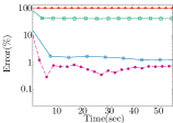
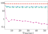
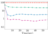
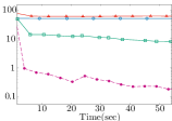
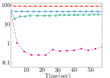
We compare the sampling algorithms VSamp, ESamp+ eBFC, ESamp+ Fast-eBFC, and WSamp. A sampling algorithm immediately starts producing estimates that get better as more iterations are executed. We record the number of iterations and relative percent error of sampling algorithms up to 60 seconds. Figure 5 shows the relative percent error with respect to the runtime for five large bipartite graphs. We report the median error of the 30 trials of sampling methods for each data point.

Our experiments show that VSamp performs poorly when compared with ESamp and WSamp under the same time budget – this is along expected lines, based on our analysis of the variance. The accuracy of ESamp  and WSamp  are comparable, with ESamp  being slightly better. Note that ESamp has a better variance, while WSamp has faster iterations. For instance, on the Wiki-en network, 1000 iters of WSamp  yields $51\%$ error in $0.13$ secs, whereas 1000 iters of ESamp yields $29\%$ error in $33$ seconds. Across all the graphs, ESamp using Fast-eBFC , which combines the benefits of faster iterations with a good variance, yields the best results, and is superior to all other sampling methods; it leads to less than 1% relative error within $5$ seconds.

6 Approximation by One-Shot Sparsification

We present methods for estimating $\mathbin{\mathchoice{\vbox{\hbox{\hskip 1.29167pt\begin{picture}(1.0,1.0)\roundcap\put(0.0,0.27){\line(1,0){1.0}} \put(1.0,0.27){\line(-1,1){1.0}} \put(0.0,1.27){\line(1,0){1.0}} \put(0.0,0.27){\line(1,1){1.0}} \end{picture}\hskip 1.29167pt\vspace{-0.6ex} }}}{\vbox{\hbox{\hskip 1.29167pt\begin{picture}(1.0,1.0)\roundcap\put(0.0,0.27){\line(1,0){1.0}} \put(1.0,0.27){\line(-1,1){1.0}} \put(0.0,1.27){\line(1,0){1.0}} \put(0.0,0.27){\line(1,1){1.0}} \end{picture}\hskip 1.29167pt\vspace{-0.6ex} }}}{\vbox{\hbox{\hskip 1.29167pt\begin{picture}(1.0,1.0)\roundcap\put(0.0,0.27){\line(1,0){1.0}} \put(1.0,0.27){\line(-1,1){1.0}} \put(0.0,1.27){\line(1,0){1.0}} \put(0.0,0.27){\line(1,1){1.0}} \end{picture}\hskip 1.29167pt\vspace{-0.6ex} }}}{\vbox{\hbox{\hskip 1.29167pt\begin{picture}(1.0,1.0)\roundcap\put(0.0,0.27){\line(1,0){1.0}} \put(1.0,0.27){\line(-1,1){1.0}} \put(0.0,1.27){\line(1,0){1.0}} \put(0.0,0.27){\line(1,1){1.0}} \end{picture}\hskip 1.29167pt\vspace{-0.6ex} }}}}(G)$ using one-shot sparsification – where we thin down the input graph into a smaller graph through a global sampling step. The number of butterflies in the sparsified graph is used to estimate $\mathbin{\mathchoice{\vbox{\hbox{\hskip 1.29167pt\begin{picture}(1.0,1.0)\roundcap\put(0.0,0.27){\line(1,0){1.0}} \put(1.0,0.27){\line(-1,1){1.0}} \put(0.0,1.27){\line(1,0){1.0}} \put(0.0,0.27){\line(1,1){1.0}} \end{picture}\hskip 1.29167pt\vspace{-0.6ex} }}}{\vbox{\hbox{\hskip 1.29167pt\begin{picture}(1.0,1.0)\roundcap\put(0.0,0.27){\line(1,0){1.0}} \put(1.0,0.27){\line(-1,1){1.0}} \put(0.0,1.27){\line(1,0){1.0}} \put(0.0,0.27){\line(1,1){1.0}} \end{picture}\hskip 1.29167pt\vspace{-0.6ex} }}}{\vbox{\hbox{\hskip 1.29167pt\begin{picture}(1.0,1.0)\roundcap\put(0.0,0.27){\line(1,0){1.0}} \put(1.0,0.27){\line(-1,1){1.0}} \put(0.0,1.27){\line(1,0){1.0}} \put(0.0,0.27){\line(1,1){1.0}} \end{picture}\hskip 1.29167pt\vspace{-0.6ex} }}}{\vbox{\hbox{\hskip 1.29167pt\begin{picture}(1.0,1.0)\roundcap\put(0.0,0.27){\line(1,0){1.0}} \put(1.0,0.27){\line(-1,1){1.0}} \put(0.0,1.27){\line(1,0){1.0}} \put(0.0,0.27){\line(1,1){1.0}} \end{picture}\hskip 1.29167pt\vspace{-0.6ex} }}}}(G)$. Unlike algorithms such as ESamp and WSamp, which work on a small subgraph constructed around a single randomly sampled edge or a wedge, sparsification methods put each edge in the graph into the sample with a certain probability. We consider two approaches to sparsification (1) ESpar in Section 6.1, where edges are chosen independently of each other and (2) ClrSpar in Section 6.2, based on a sampling method where different edges are not independently chosen, but dense regions appear with higher probability in the sample – based on a similar idea in the context of triangle counting due to Pagh and Tsourakakis Pagh and Tsourakakis (2012).

(a)

(b)

(c)

(d)

(e)

Figure 6: Accuracy (on left y-axis) and runtime performance (on right y-axis) of sparsification algorithms for different probabilities (on x-axis). ESpar performs better than ClrSpar, and yields $<1\%$ relative error within $4$ seconds for all networks.

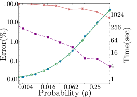
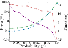
6.1 Edge Sparsification (ESpar)

In ESpar, the input graph $G$ is sparsified by independently retaining each edge in $G$ in the sampled graph $G^{\prime}$, with a probability $p$. The number of butterflies in $G^{\prime}$, obtained using ExactBFC, is used to construct an estimate of $\mathbin{\mathchoice{\vbox{\hbox{\hskip 1.29167pt\begin{picture}(1.0,1.0)\roundcap\put(0.0,0.27){\line(1,0){1.0}} \put(1.0,0.27){\line(-1,1){1.0}} \put(0.0,1.27){\line(1,0){1.0}} \put(0.0,0.27){\line(1,1){1.0}} \end{picture}\hskip 1.29167pt\vspace{-0.6ex} }}}{\vbox{\hbox{\hskip 1.29167pt\begin{picture}(1.0,1.0)\roundcap\put(0.0,0.27){\line(1,0){1.0}} \put(1.0,0.27){\line(-1,1){1.0}} \put(0.0,1.27){\line(1,0){1.0}} \put(0.0,0.27){\line(1,1){1.0}} \end{picture}\hskip 1.29167pt\vspace{-0.6ex} }}}{\vbox{\hbox{\hskip 1.29167pt\begin{picture}(1.0,1.0)\roundcap\put(0.0,0.27){\line(1,0){1.0}} \put(1.0,0.27){\line(-1,1){1.0}} \put(0.0,1.27){\line(1,0){1.0}} \put(0.0,0.27){\line(1,1){1.0}} \end{picture}\hskip 1.29167pt\vspace{-0.6ex} }}}{\vbox{\hbox{\hskip 1.29167pt\begin{picture}(1.0,1.0)\roundcap\put(0.0,0.27){\line(1,0){1.0}} \put(1.0,0.27){\line(-1,1){1.0}} \put(0.0,1.27){\line(1,0){1.0}} \put(0.0,0.27){\line(1,1){1.0}} \end{picture}\hskip 1.29167pt\vspace{-0.6ex} }}}}(G)$, after applying a scaling factor. This is much faster than working with the original graph $G$ since the number of edges in $G^{\prime}$ can be much smaller. The ESpar algorithm is described in Algorithm 8.

Input : A bipartite graph $G=(V,E)$, parameter $p,0<p<1$

1 Construct $E^{\prime}$ by including each edge $e\in E$ independently with probability $p$

2

3$\beta\leftarrow{\textsc{ExactBFC}}(V,E^{\prime})$ using Algorithm 1

4 return $\beta\times p^{-4}$

Algorithm 8 ESpar: Edge Sparsification

Lemma 15.

Let $Y_{ES}$ denote the output of ESpar on input graph $G$. Then ${\mathbb{E}}\left[Y_{ES}\right]=\mathbin{\mathchoice{\vbox{\hbox{\hskip 1.29167pt\begin{picture}(1.0,1.0)\roundcap\put(0.0,0.27){\line(1,0){1.0}} \put(1.0,0.27){\line(-1,1){1.0}} \put(0.0,1.27){\line(1,0){1.0}} \put(0.0,0.27){\line(1,1){1.0}} \end{picture}\hskip 1.29167pt\vspace{-0.6ex} }}}{\vbox{\hbox{\hskip 1.29167pt\begin{picture}(1.0,1.0)\roundcap\put(0.0,0.27){\line(1,0){1.0}} \put(1.0,0.27){\line(-1,1){1.0}} \put(0.0,1.27){\line(1,0){1.0}} \put(0.0,0.27){\line(1,1){1.0}} \end{picture}\hskip 1.29167pt\vspace{-0.6ex} }}}{\vbox{\hbox{\hskip 1.29167pt\begin{picture}(1.0,1.0)\roundcap\put(0.0,0.27){\line(1,0){1.0}} \put(1.0,0.27){\line(-1,1){1.0}} \put(0.0,1.27){\line(1,0){1.0}} \put(0.0,0.27){\line(1,1){1.0}} \end{picture}\hskip 1.29167pt\vspace{-0.6ex} }}}{\vbox{\hbox{\hskip 1.29167pt\begin{picture}(1.0,1.0)\roundcap\put(0.0,0.27){\line(1,0){1.0}} \put(1.0,0.27){\line(-1,1){1.0}} \put(0.0,1.27){\line(1,0){1.0}} \put(0.0,0.27){\line(1,1){1.0}} \end{picture}\hskip 1.29167pt\vspace{-0.6ex} }}}}(G)$. If $p>\max\left(\sqrt[4]{\frac{24}{\mathbin{\mathchoice{\vbox{\hbox{\hskip 1.29167pt\begin{picture}(1.0,1.0)\roundcap\put(0.0,0.27){\line(1,0){1.0}} \put(1.0,0.27){\line(-1,1){1.0}} \put(0.0,1.27){\line(1,0){1.0}} \put(0.0,0.27){\line(1,1){1.0}} \end{picture}\hskip 1.29167pt\vspace{-0.6ex} }}}{\vbox{\hbox{\hskip 1.29167pt\begin{picture}(1.0,1.0)\roundcap\put(0.0,0.27){\line(1,0){1.0}} \put(1.0,0.27){\line(-1,1){1.0}} \put(0.0,1.27){\line(1,0){1.0}} \put(0.0,0.27){\line(1,1){1.0}} \end{picture}\hskip 1.29167pt\vspace{-0.6ex} }}}{\vbox{\hbox{\hskip 1.29167pt\begin{picture}(1.0,1.0)\roundcap\put(0.0,0.27){\line(1,0){1.0}} \put(1.0,0.27){\line(-1,1){1.0}} \put(0.0,1.27){\line(1,0){1.0}} \put(0.0,0.27){\line(1,1){1.0}} \end{picture}\hskip 1.29167pt\vspace{-0.6ex} }}}{\vbox{\hbox{\hskip 1.29167pt\begin{picture}(1.0,1.0)\roundcap\put(0.0,0.27){\line(1,0){1.0}} \put(1.0,0.27){\line(-1,1){1.0}} \put(0.0,1.27){\line(1,0){1.0}} \put(0.0,0.27){\line(1,1){1.0}} \end{picture}\hskip 1.29167pt\vspace{-0.6ex} }}}}}},\sqrt{\frac{24\Delta}{\mathbin{\mathchoice{\vbox{\hbox{\hskip 1.29167pt\begin{picture}(1.0,1.0)\roundcap\put(0.0,0.27){\line(1,0){1.0}} \put(1.0,0.27){\line(-1,1){1.0}} \put(0.0,1.27){\line(1,0){1.0}} \put(0.0,0.27){\line(1,1){1.0}} \end{picture}\hskip 1.29167pt\vspace{-0.6ex} }}}{\vbox{\hbox{\hskip 1.29167pt\begin{picture}(1.0,1.0)\roundcap\put(0.0,0.27){\line(1,0){1.0}} \put(1.0,0.27){\line(-1,1){1.0}} \put(0.0,1.27){\line(1,0){1.0}} \put(0.0,0.27){\line(1,1){1.0}} \end{picture}\hskip 1.29167pt\vspace{-0.6ex} }}}{\vbox{\hbox{\hskip 1.29167pt\begin{picture}(1.0,1.0)\roundcap\put(0.0,0.27){\line(1,0){1.0}} \put(1.0,0.27){\line(-1,1){1.0}} \put(0.0,1.27){\line(1,0){1.0}} \put(0.0,0.27){\line(1,1){1.0}} \end{picture}\hskip 1.29167pt\vspace{-0.6ex} }}}{\vbox{\hbox{\hskip 1.29167pt\begin{picture}(1.0,1.0)\roundcap\put(0.0,0.27){\line(1,0){1.0}} \put(1.0,0.27){\line(-1,1){1.0}} \put(0.0,1.27){\line(1,0){1.0}} \put(0.0,0.27){\line(1,1){1.0}} \end{picture}\hskip 1.29167pt\vspace{-0.6ex} }}}}}},\frac{24\Delta^{2}}{\mathbin{\mathchoice{\vbox{\hbox{\hskip 1.29167pt\begin{picture}(1.0,1.0)\roundcap\put(0.0,0.27){\line(1,0){1.0}} \put(1.0,0.27){\line(-1,1){1.0}} \put(0.0,1.27){\line(1,0){1.0}} \put(0.0,0.27){\line(1,1){1.0}} \end{picture}\hskip 1.29167pt\vspace{-0.6ex} }}}{\vbox{\hbox{\hskip 1.29167pt\begin{picture}(1.0,1.0)\roundcap\put(0.0,0.27){\line(1,0){1.0}} \put(1.0,0.27){\line(-1,1){1.0}} \put(0.0,1.27){\line(1,0){1.0}} \put(0.0,0.27){\line(1,1){1.0}} \end{picture}\hskip 1.29167pt\vspace{-0.6ex} }}}{\vbox{\hbox{\hskip 1.29167pt\begin{picture}(1.0,1.0)\roundcap\put(0.0,0.27){\line(1,0){1.0}} \put(1.0,0.27){\line(-1,1){1.0}} \put(0.0,1.27){\line(1,0){1.0}} \put(0.0,0.27){\line(1,1){1.0}} \end{picture}\hskip 1.29167pt\vspace{-0.6ex} }}}{\vbox{\hbox{\hskip 1.29167pt\begin{picture}(1.0,1.0)\roundcap\put(0.0,0.27){\line(1,0){1.0}} \put(1.0,0.27){\line(-1,1){1.0}} \put(0.0,1.27){\line(1,0){1.0}} \put(0.0,0.27){\line(1,1){1.0}} \end{picture}\hskip 1.29167pt\vspace{-0.6ex} }}}}}\right)$, then $\mathbb{V}\mathrm{ar}\left[Y_{ES}\right]\leq\mathbin{\mathchoice{\vbox{\hbox{\hskip 1.29167pt\begin{picture}(1.0,1.0)\roundcap\put(0.0,0.27){\line(1,0){1.0}} \put(1.0,0.27){\line(-1,1){1.0}} \put(0.0,1.27){\line(1,0){1.0}} \put(0.0,0.27){\line(1,1){1.0}} \end{picture}\hskip 1.29167pt\vspace{-0.6ex} }}}{\vbox{\hbox{\hskip 1.29167pt\begin{picture}(1.0,1.0)\roundcap\put(0.0,0.27){\line(1,0){1.0}} \put(1.0,0.27){\line(-1,1){1.0}} \put(0.0,1.27){\line(1,0){1.0}} \put(0.0,0.27){\line(1,1){1.0}} \end{picture}\hskip 1.29167pt\vspace{-0.6ex} }}}{\vbox{\hbox{\hskip 1.29167pt\begin{picture}(1.0,1.0)\roundcap\put(0.0,0.27){\line(1,0){1.0}} \put(1.0,0.27){\line(-1,1){1.0}} \put(0.0,1.27){\line(1,0){1.0}} \put(0.0,0.27){\line(1,1){1.0}} \end{picture}\hskip 1.29167pt\vspace{-0.6ex} }}}{\vbox{\hbox{\hskip 1.29167pt\begin{picture}(1.0,1.0)\roundcap\put(0.0,0.27){\line(1,0){1.0}} \put(1.0,0.27){\line(-1,1){1.0}} \put(0.0,1.27){\line(1,0){1.0}} \put(0.0,0.27){\line(1,1){1.0}} \end{picture}\hskip 1.29167pt\vspace{-0.6ex} }}}}^{2}/8$.

Proof.

For $i=1,\cdots,\mathbin{\mathchoice{\vbox{\hbox{\hskip 1.29167pt\begin{picture}(1.0,1.0)\roundcap\put(0.0,0.27){\line(1,0){1.0}} \put(1.0,0.27){\line(-1,1){1.0}} \put(0.0,1.27){\line(1,0){1.0}} \put(0.0,0.27){\line(1,1){1.0}} \end{picture}\hskip 1.29167pt\vspace{-0.6ex} }}}{\vbox{\hbox{\hskip 1.29167pt\begin{picture}(1.0,1.0)\roundcap\put(0.0,0.27){\line(1,0){1.0}} \put(1.0,0.27){\line(-1,1){1.0}} \put(0.0,1.27){\line(1,0){1.0}} \put(0.0,0.27){\line(1,1){1.0}} \end{picture}\hskip 1.29167pt\vspace{-0.6ex} }}}{\vbox{\hbox{\hskip 1.29167pt\begin{picture}(1.0,1.0)\roundcap\put(0.0,0.27){\line(1,0){1.0}} \put(1.0,0.27){\line(-1,1){1.0}} \put(0.0,1.27){\line(1,0){1.0}} \put(0.0,0.27){\line(1,1){1.0}} \end{picture}\hskip 1.29167pt\vspace{-0.6ex} }}}{\vbox{\hbox{\hskip 1.29167pt\begin{picture}(1.0,1.0)\roundcap\put(0.0,0.27){\line(1,0){1.0}} \put(1.0,0.27){\line(-1,1){1.0}} \put(0.0,1.27){\line(1,0){1.0}} \put(0.0,0.27){\line(1,1){1.0}} \end{picture}\hskip 1.29167pt\vspace{-0.6ex} }}}}$, let $X_{i}$ be a random variable indicating the $i^{th}$ butterfly, s.t. $X_{i}$ is $1$ if the $i^{th}$ butterfly exists in the sampled graph $(V_{G},E^{\prime})$ and $0$ otherwise. Let $\beta$ be as defined in the algorithm. Clearly, $\beta=\sum_{i=1}^{\mathbin{\mathchoice{\vbox{\hbox{\hskip 1.29167pt\begin{picture}(1.0,1.0)\roundcap\put(0.0,0.27){\line(1,0){1.0}} \put(1.0,0.27){\line(-1,1){1.0}} \put(0.0,1.27){\line(1,0){1.0}} \put(0.0,0.27){\line(1,1){1.0}} \end{picture}\hskip 1.29167pt\vspace{-0.6ex} }}}{\vbox{\hbox{\hskip 1.29167pt\begin{picture}(1.0,1.0)\roundcap\put(0.0,0.27){\line(1,0){1.0}} \put(1.0,0.27){\line(-1,1){1.0}} \put(0.0,1.27){\line(1,0){1.0}} \put(0.0,0.27){\line(1,1){1.0}} \end{picture}\hskip 1.29167pt\vspace{-0.6ex} }}}{\vbox{\hbox{\hskip 1.29167pt\begin{picture}(1.0,1.0)\roundcap\put(0.0,0.27){\line(1,0){1.0}} \put(1.0,0.27){\line(-1,1){1.0}} \put(0.0,1.27){\line(1,0){1.0}} \put(0.0,0.27){\line(1,1){1.0}} \end{picture}\hskip 1.29167pt\vspace{-0.6ex} }}}{\vbox{\hbox{\hskip 1.29167pt\begin{picture}(1.0,1.0)\roundcap\put(0.0,0.27){\line(1,0){1.0}} \put(1.0,0.27){\line(-1,1){1.0}} \put(0.0,1.27){\line(1,0){1.0}} \put(0.0,0.27){\line(1,1){1.0}} \end{picture}\hskip 1.29167pt\vspace{-0.6ex} }}}}}X_{i}$. We have ${\mathbb{E}}\left[\beta\right]=\sum{\mathbb{E}}\left[X_{i}\right]=\sum{\Pr}\left[X_{i}=1\right]$. Since different edges are sampled independently, we have ${\Pr}\left[X_{i}=1\right]=p^{4}$. Hence, ${\mathbb{E}}\left[Y_{ES}\right]=p^{-4}{\mathbb{E}}\left[\beta\right]=p^{-4}\sum_{i=1}^{\mathbin{\mathchoice{\vbox{\hbox{\hskip 1.29167pt\begin{picture}(1.0,1.0)\roundcap\put(0.0,0.27){\line(1,0){1.0}} \put(1.0,0.27){\line(-1,1){1.0}} \put(0.0,1.27){\line(1,0){1.0}} \put(0.0,0.27){\line(1,1){1.0}} \end{picture}\hskip 1.29167pt\vspace{-0.6ex} }}}{\vbox{\hbox{\hskip 1.29167pt\begin{picture}(1.0,1.0)\roundcap\put(0.0,0.27){\line(1,0){1.0}} \put(1.0,0.27){\line(-1,1){1.0}} \put(0.0,1.27){\line(1,0){1.0}} \put(0.0,0.27){\line(1,1){1.0}} \end{picture}\hskip 1.29167pt\vspace{-0.6ex} }}}{\vbox{\hbox{\hskip 1.29167pt\begin{picture}(1.0,1.0)\roundcap\put(0.0,0.27){\line(1,0){1.0}} \put(1.0,0.27){\line(-1,1){1.0}} \put(0.0,1.27){\line(1,0){1.0}} \put(0.0,0.27){\line(1,1){1.0}} \end{picture}\hskip 1.29167pt\vspace{-0.6ex} }}}{\vbox{\hbox{\hskip 1.29167pt\begin{picture}(1.0,1.0)\roundcap\put(0.0,0.27){\line(1,0){1.0}} \put(1.0,0.27){\line(-1,1){1.0}} \put(0.0,1.27){\line(1,0){1.0}} \put(0.0,0.27){\line(1,1){1.0}} \end{picture}\hskip 1.29167pt\vspace{-0.6ex} }}}}}p^{4}=\mathbin{\mathchoice{\vbox{\hbox{\hskip 1.29167pt\begin{picture}(1.0,1.0)\roundcap\put(0.0,0.27){\line(1,0){1.0}} \put(1.0,0.27){\line(-1,1){1.0}} \put(0.0,1.27){\line(1,0){1.0}} \put(0.0,0.27){\line(1,1){1.0}} \end{picture}\hskip 1.29167pt\vspace{-0.6ex} }}}{\vbox{\hbox{\hskip 1.29167pt\begin{picture}(1.0,1.0)\roundcap\put(0.0,0.27){\line(1,0){1.0}} \put(1.0,0.27){\line(-1,1){1.0}} \put(0.0,1.27){\line(1,0){1.0}} \put(0.0,0.27){\line(1,1){1.0}} \end{picture}\hskip 1.29167pt\vspace{-0.6ex} }}}{\vbox{\hbox{\hskip 1.29167pt\begin{picture}(1.0,1.0)\roundcap\put(0.0,0.27){\line(1,0){1.0}} \put(1.0,0.27){\line(-1,1){1.0}} \put(0.0,1.27){\line(1,0){1.0}} \put(0.0,0.27){\line(1,1){1.0}} \end{picture}\hskip 1.29167pt\vspace{-0.6ex} }}}{\vbox{\hbox{\hskip 1.29167pt\begin{picture}(1.0,1.0)\roundcap\put(0.0,0.27){\line(1,0){1.0}} \put(1.0,0.27){\line(-1,1){1.0}} \put(0.0,1.27){\line(1,0){1.0}} \put(0.0,0.27){\line(1,1){1.0}} \end{picture}\hskip 1.29167pt\vspace{-0.6ex} }}}}$.

The random variables $X_{i}$s corresponding to different butterflies are not independent of each other, since butterflies may share edges. Accounting for the covariances of $X_{i},X_{j}$ pairs leads to:

$$\mathbb{V}\mathrm{ar}[Y_{ES}] =\mathbb{V}\mathrm{ar}\left[p^{-4}\sum_{i=1}^{\mathbin{\mathchoice{\vbox{\hbox{\hskip 1.29167pt\begin{picture}(1.0,1.0)\roundcap\put(0.0,0.27){\line(1,0){1.0}} \put(1.0,0.27){\line(-1,1){1.0}} \put(0.0,1.27){\line(1,0){1.0}} \put(0.0,0.27){\line(1,1){1.0}} \end{picture}\hskip 1.29167pt\vspace{-0.6ex} }}}{\vbox{\hbox{\hskip 1.29167pt\begin{picture}(1.0,1.0)\roundcap\put(0.0,0.27){\line(1,0){1.0}} \put(1.0,0.27){\line(-1,1){1.0}} \put(0.0,1.27){\line(1,0){1.0}} \put(0.0,0.27){\line(1,1){1.0}} \end{picture}\hskip 1.29167pt\vspace{-0.6ex} }}}{\vbox{\hbox{\hskip 1.29167pt\begin{picture}(1.0,1.0)\roundcap\put(0.0,0.27){\line(1,0){1.0}} \put(1.0,0.27){\line(-1,1){1.0}} \put(0.0,1.27){\line(1,0){1.0}} \put(0.0,0.27){\line(1,1){1.0}} \end{picture}\hskip 1.29167pt\vspace{-0.6ex} }}}{\vbox{\hbox{\hskip 1.29167pt\begin{picture}(1.0,1.0)\roundcap\put(0.0,0.27){\line(1,0){1.0}} \put(1.0,0.27){\line(-1,1){1.0}} \put(0.0,1.27){\line(1,0){1.0}} \put(0.0,0.27){\line(1,1){1.0}} \end{picture}\hskip 1.29167pt\vspace{-0.6ex} }}}}}{X_{i}}\right]$$

$$=p^{-8}\left[\sum_{i=1}^{\mathbin{\mathchoice{\vbox{\hbox{\hskip 1.29167pt\begin{picture}(1.0,1.0)\roundcap\put(0.0,0.27){\line(1,0){1.0}} \put(1.0,0.27){\line(-1,1){1.0}} \put(0.0,1.27){\line(1,0){1.0}} \put(0.0,0.27){\line(1,1){1.0}} \end{picture}\hskip 1.29167pt\vspace{-0.6ex} }}}{\vbox{\hbox{\hskip 1.29167pt\begin{picture}(1.0,1.0)\roundcap\put(0.0,0.27){\line(1,0){1.0}} \put(1.0,0.27){\line(-1,1){1.0}} \put(0.0,1.27){\line(1,0){1.0}} \put(0.0,0.27){\line(1,1){1.0}} \end{picture}\hskip 1.29167pt\vspace{-0.6ex} }}}{\vbox{\hbox{\hskip 1.29167pt\begin{picture}(1.0,1.0)\roundcap\put(0.0,0.27){\line(1,0){1.0}} \put(1.0,0.27){\line(-1,1){1.0}} \put(0.0,1.27){\line(1,0){1.0}} \put(0.0,0.27){\line(1,1){1.0}} \end{picture}\hskip 1.29167pt\vspace{-0.6ex} }}}{\vbox{\hbox{\hskip 1.29167pt\begin{picture}(1.0,1.0)\roundcap\put(0.0,0.27){\line(1,0){1.0}} \put(1.0,0.27){\line(-1,1){1.0}} \put(0.0,1.27){\line(1,0){1.0}} \put(0.0,0.27){\line(1,1){1.0}} \end{picture}\hskip 1.29167pt\vspace{-0.6ex} }}}}}{(\mathbb{E}[X_{i}]-\mathbb{E}^{2}[X_{i}])}+\sum_{i\neq j}{\mathbb{C}\mathrm{ov}(X_{i}\wedge X_{j})}\right]$$

$$=p^{-8}\left[\mathbin{\mathchoice{\vbox{\hbox{\hskip 1.29167pt\begin{picture}(1.0,1.0)\roundcap\put(0.0,0.27){\line(1,0){1.0}} \put(1.0,0.27){\line(-1,1){1.0}} \put(0.0,1.27){\line(1,0){1.0}} \put(0.0,0.27){\line(1,1){1.0}} \end{picture}\hskip 1.29167pt\vspace{-0.6ex} }}}{\vbox{\hbox{\hskip 1.29167pt\begin{picture}(1.0,1.0)\roundcap\put(0.0,0.27){\line(1,0){1.0}} \put(1.0,0.27){\line(-1,1){1.0}} \put(0.0,1.27){\line(1,0){1.0}} \put(0.0,0.27){\line(1,1){1.0}} \end{picture}\hskip 1.29167pt\vspace{-0.6ex} }}}{\vbox{\hbox{\hskip 1.29167pt\begin{picture}(1.0,1.0)\roundcap\put(0.0,0.27){\line(1,0){1.0}} \put(1.0,0.27){\line(-1,1){1.0}} \put(0.0,1.27){\line(1,0){1.0}} \put(0.0,0.27){\line(1,1){1.0}} \end{picture}\hskip 1.29167pt\vspace{-0.6ex} }}}{\vbox{\hbox{\hskip 1.29167pt\begin{picture}(1.0,1.0)\roundcap\put(0.0,0.27){\line(1,0){1.0}} \put(1.0,0.27){\line(-1,1){1.0}} \put(0.0,1.27){\line(1,0){1.0}} \put(0.0,0.27){\line(1,1){1.0}} \end{picture}\hskip 1.29167pt\vspace{-0.6ex} }}}}(p^{4}-p^{8})+\sum_{i\neq j}{(\mathbb{E}[X_{i}X_{j}]-\mathbb{E}[X_{i}]\mathbb{E}[X_{j}])}\right]$$

Let $p_{0e},p_{1e}$, and $p_{1w}$ respectively denote the number of pairs of butterflies that share zero edges, one edge, and one wedge (two edges). Note that these three cases account for all pairs of distinct butterflies, since it is not possible for two distinct butterflies to share three or more edges. Proceeding with a calculation similar to ones in Section 5, we get:

$$\mathbb{V}\mathrm{ar}[Y_{ES}] =p^{-8}\left[\mathbin{\mathchoice{\vbox{\hbox{\hskip 1.29167pt\begin{picture}(1.0,1.0)\roundcap\put(0.0,0.27){\line(1,0){1.0}} \put(1.0,0.27){\line(-1,1){1.0}} \put(0.0,1.27){\line(1,0){1.0}} \put(0.0,0.27){\line(1,1){1.0}} \end{picture}\hskip 1.29167pt\vspace{-0.6ex} }}}{\vbox{\hbox{\hskip 1.29167pt\begin{picture}(1.0,1.0)\roundcap\put(0.0,0.27){\line(1,0){1.0}} \put(1.0,0.27){\line(-1,1){1.0}} \put(0.0,1.27){\line(1,0){1.0}} \put(0.0,0.27){\line(1,1){1.0}} \end{picture}\hskip 1.29167pt\vspace{-0.6ex} }}}{\vbox{\hbox{\hskip 1.29167pt\begin{picture}(1.0,1.0)\roundcap\put(0.0,0.27){\line(1,0){1.0}} \put(1.0,0.27){\line(-1,1){1.0}} \put(0.0,1.27){\line(1,0){1.0}} \put(0.0,0.27){\line(1,1){1.0}} \end{picture}\hskip 1.29167pt\vspace{-0.6ex} }}}{\vbox{\hbox{\hskip 1.29167pt\begin{picture}(1.0,1.0)\roundcap\put(0.0,0.27){\line(1,0){1.0}} \put(1.0,0.27){\line(-1,1){1.0}} \put(0.0,1.27){\line(1,0){1.0}} \put(0.0,0.27){\line(1,1){1.0}} \end{picture}\hskip 1.29167pt\vspace{-0.6ex} }}}}(p^{4}-p^{8})+p_{1e}(p^{7}-p^{8})+p_{1w}(p^{6}-p^{8})\right]$$

$$\leq\leavevmode\nobreak\ {}\mathbin{\mathchoice{\vbox{\hbox{\hskip 1.29167pt\begin{picture}(1.0,1.0)\roundcap\put(0.0,0.27){\line(1,0){1.0}} \put(1.0,0.27){\line(-1,1){1.0}} \put(0.0,1.27){\line(1,0){1.0}} \put(0.0,0.27){\line(1,1){1.0}} \end{picture}\hskip 1.29167pt\vspace{-0.6ex} }}}{\vbox{\hbox{\hskip 1.29167pt\begin{picture}(1.0,1.0)\roundcap\put(0.0,0.27){\line(1,0){1.0}} \put(1.0,0.27){\line(-1,1){1.0}} \put(0.0,1.27){\line(1,0){1.0}} \put(0.0,0.27){\line(1,1){1.0}} \end{picture}\hskip 1.29167pt\vspace{-0.6ex} }}}{\vbox{\hbox{\hskip 1.29167pt\begin{picture}(1.0,1.0)\roundcap\put(0.0,0.27){\line(1,0){1.0}} \put(1.0,0.27){\line(-1,1){1.0}} \put(0.0,1.27){\line(1,0){1.0}} \put(0.0,0.27){\line(1,1){1.0}} \end{picture}\hskip 1.29167pt\vspace{-0.6ex} }}}{\vbox{\hbox{\hskip 1.29167pt\begin{picture}(1.0,1.0)\roundcap\put(0.0,0.27){\line(1,0){1.0}} \put(1.0,0.27){\line(-1,1){1.0}} \put(0.0,1.27){\line(1,0){1.0}} \put(0.0,0.27){\line(1,1){1.0}} \end{picture}\hskip 1.29167pt\vspace{-0.6ex} }}}}{}p^{-4}+p_{1w}p^{-2}+p_{1e}p^{-1}$$

By Chebyshev’s inequality we have $\Pr[|Y_{ES}-\mathbin{\mathchoice{\vbox{\hbox{\hskip 1.29167pt\begin{picture}(1.0,1.0)\roundcap\put(0.0,0.27){\line(1,0){1.0}} \put(1.0,0.27){\line(-1,1){1.0}} \put(0.0,1.27){\line(1,0){1.0}} \put(0.0,0.27){\line(1,1){1.0}} \end{picture}\hskip 1.29167pt\vspace{-0.6ex} }}}{\vbox{\hbox{\hskip 1.29167pt\begin{picture}(1.0,1.0)\roundcap\put(0.0,0.27){\line(1,0){1.0}} \put(1.0,0.27){\line(-1,1){1.0}} \put(0.0,1.27){\line(1,0){1.0}} \put(0.0,0.27){\line(1,1){1.0}} \end{picture}\hskip 1.29167pt\vspace{-0.6ex} }}}{\vbox{\hbox{\hskip 1.29167pt\begin{picture}(1.0,1.0)\roundcap\put(0.0,0.27){\line(1,0){1.0}} \put(1.0,0.27){\line(-1,1){1.0}} \put(0.0,1.27){\line(1,0){1.0}} \put(0.0,0.27){\line(1,1){1.0}} \end{picture}\hskip 1.29167pt\vspace{-0.6ex} }}}{\vbox{\hbox{\hskip 1.29167pt\begin{picture}(1.0,1.0)\roundcap\put(0.0,0.27){\line(1,0){1.0}} \put(1.0,0.27){\line(-1,1){1.0}} \put(0.0,1.27){\line(1,0){1.0}} \put(0.0,0.27){\line(1,1){1.0}} \end{picture}\hskip 1.29167pt\vspace{-0.6ex} }}}}|\geq\epsilon\mathbin{\mathchoice{\vbox{\hbox{\hskip 1.29167pt\begin{picture}(1.0,1.0)\roundcap\put(0.0,0.27){\line(1,0){1.0}} \put(1.0,0.27){\line(-1,1){1.0}} \put(0.0,1.27){\line(1,0){1.0}} \put(0.0,0.27){\line(1,1){1.0}} \end{picture}\hskip 1.29167pt\vspace{-0.6ex} }}}{\vbox{\hbox{\hskip 1.29167pt\begin{picture}(1.0,1.0)\roundcap\put(0.0,0.27){\line(1,0){1.0}} \put(1.0,0.27){\line(-1,1){1.0}} \put(0.0,1.27){\line(1,0){1.0}} \put(0.0,0.27){\line(1,1){1.0}} \end{picture}\hskip 1.29167pt\vspace{-0.6ex} }}}{\vbox{\hbox{\hskip 1.29167pt\begin{picture}(1.0,1.0)\roundcap\put(0.0,0.27){\line(1,0){1.0}} \put(1.0,0.27){\line(-1,1){1.0}} \put(0.0,1.27){\line(1,0){1.0}} \put(0.0,0.27){\line(1,1){1.0}} \end{picture}\hskip 1.29167pt\vspace{-0.6ex} }}}{\vbox{\hbox{\hskip 1.29167pt\begin{picture}(1.0,1.0)\roundcap\put(0.0,0.27){\line(1,0){1.0}} \put(1.0,0.27){\line(-1,1){1.0}} \put(0.0,1.27){\line(1,0){1.0}} \put(0.0,0.27){\line(1,1){1.0}} \end{picture}\hskip 1.29167pt\vspace{-0.6ex} }}}}]\leq\frac{\mathbb{V}\mathrm{ar}[Y_{ES}]}{\epsilon^{2}\mathbb{E}^{2}[Y_{ES}]}$. We need to find the probability $p$ such that $\mathbb{V}\mathrm{ar}[Y_{ES}]=o(\mathbb{E}^{2}[Y_{ES}])$ which results in $\mathbb{E}[Y_{ES}]=\leavevmode\nobreak\ {}\mathbin{\mathchoice{\vbox{\hbox{\hskip 1.29167pt\begin{picture}(1.0,1.0)\roundcap\put(0.0,0.27){\line(1,0){1.0}} \put(1.0,0.27){\line(-1,1){1.0}} \put(0.0,1.27){\line(1,0){1.0}} \put(0.0,0.27){\line(1,1){1.0}} \end{picture}\hskip 1.29167pt\vspace{-0.6ex} }}}{\vbox{\hbox{\hskip 1.29167pt\begin{picture}(1.0,1.0)\roundcap\put(0.0,0.27){\line(1,0){1.0}} \put(1.0,0.27){\line(-1,1){1.0}} \put(0.0,1.27){\line(1,0){1.0}} \put(0.0,0.27){\line(1,1){1.0}} \end{picture}\hskip 1.29167pt\vspace{-0.6ex} }}}{\vbox{\hbox{\hskip 1.29167pt\begin{picture}(1.0,1.0)\roundcap\put(0.0,0.27){\line(1,0){1.0}} \put(1.0,0.27){\line(-1,1){1.0}} \put(0.0,1.27){\line(1,0){1.0}} \put(0.0,0.27){\line(1,1){1.0}} \end{picture}\hskip 1.29167pt\vspace{-0.6ex} }}}{\vbox{\hbox{\hskip 1.29167pt\begin{picture}(1.0,1.0)\roundcap\put(0.0,0.27){\line(1,0){1.0}} \put(1.0,0.27){\line(-1,1){1.0}} \put(0.0,1.27){\line(1,0){1.0}} \put(0.0,0.27){\line(1,1){1.0}} \end{picture}\hskip 1.29167pt\vspace{-0.6ex} }}}}$ with probability $1-o(1)$. Thus,

$$\mathbb{E}^{2}[Y_{ES}] \gg\mathbb{V}\mathrm{ar}[Y_{ES}]$$

$$\mathbin{\mathchoice{\vbox{\hbox{\hskip 1.29167pt\begin{picture}(1.0,1.0)\roundcap\put(0.0,0.27){\line(1,0){1.0}} \put(1.0,0.27){\line(-1,1){1.0}} \put(0.0,1.27){\line(1,0){1.0}} \put(0.0,0.27){\line(1,1){1.0}} \end{picture}\hskip 1.29167pt\vspace{-0.6ex} }}}{\vbox{\hbox{\hskip 1.29167pt\begin{picture}(1.0,1.0)\roundcap\put(0.0,0.27){\line(1,0){1.0}} \put(1.0,0.27){\line(-1,1){1.0}} \put(0.0,1.27){\line(1,0){1.0}} \put(0.0,0.27){\line(1,1){1.0}} \end{picture}\hskip 1.29167pt\vspace{-0.6ex} }}}{\vbox{\hbox{\hskip 1.29167pt\begin{picture}(1.0,1.0)\roundcap\put(0.0,0.27){\line(1,0){1.0}} \put(1.0,0.27){\line(-1,1){1.0}} \put(0.0,1.27){\line(1,0){1.0}} \put(0.0,0.27){\line(1,1){1.0}} \end{picture}\hskip 1.29167pt\vspace{-0.6ex} }}}{\vbox{\hbox{\hskip 1.29167pt\begin{picture}(1.0,1.0)\roundcap\put(0.0,0.27){\line(1,0){1.0}} \put(1.0,0.27){\line(-1,1){1.0}} \put(0.0,1.27){\line(1,0){1.0}} \put(0.0,0.27){\line(1,1){1.0}} \end{picture}\hskip 1.29167pt\vspace{-0.6ex} }}}}^{2} \gg\leavevmode\nobreak\ {}\mathbin{\mathchoice{\vbox{\hbox{\hskip 1.29167pt\begin{picture}(1.0,1.0)\roundcap\put(0.0,0.27){\line(1,0){1.0}} \put(1.0,0.27){\line(-1,1){1.0}} \put(0.0,1.27){\line(1,0){1.0}} \put(0.0,0.27){\line(1,1){1.0}} \end{picture}\hskip 1.29167pt\vspace{-0.6ex} }}}{\vbox{\hbox{\hskip 1.29167pt\begin{picture}(1.0,1.0)\roundcap\put(0.0,0.27){\line(1,0){1.0}} \put(1.0,0.27){\line(-1,1){1.0}} \put(0.0,1.27){\line(1,0){1.0}} \put(0.0,0.27){\line(1,1){1.0}} \end{picture}\hskip 1.29167pt\vspace{-0.6ex} }}}{\vbox{\hbox{\hskip 1.29167pt\begin{picture}(1.0,1.0)\roundcap\put(0.0,0.27){\line(1,0){1.0}} \put(1.0,0.27){\line(-1,1){1.0}} \put(0.0,1.27){\line(1,0){1.0}} \put(0.0,0.27){\line(1,1){1.0}} \end{picture}\hskip 1.29167pt\vspace{-0.6ex} }}}{\vbox{\hbox{\hskip 1.29167pt\begin{picture}(1.0,1.0)\roundcap\put(0.0,0.27){\line(1,0){1.0}} \put(1.0,0.27){\line(-1,1){1.0}} \put(0.0,1.27){\line(1,0){1.0}} \put(0.0,0.27){\line(1,1){1.0}} \end{picture}\hskip 1.29167pt\vspace{-0.6ex} }}}}{}p^{-4}+p_{1w}p^{-2}+p_{1e}p^{-1}-(\mathbin{\mathchoice{\vbox{\hbox{\hskip 1.29167pt\begin{picture}(1.0,1.0)\roundcap\put(0.0,0.27){\line(1,0){1.0}} \put(1.0,0.27){\line(-1,1){1.0}} \put(0.0,1.27){\line(1,0){1.0}} \put(0.0,0.27){\line(1,1){1.0}} \end{picture}\hskip 1.29167pt\vspace{-0.6ex} }}}{\vbox{\hbox{\hskip 1.29167pt\begin{picture}(1.0,1.0)\roundcap\put(0.0,0.27){\line(1,0){1.0}} \put(1.0,0.27){\line(-1,1){1.0}} \put(0.0,1.27){\line(1,0){1.0}} \put(0.0,0.27){\line(1,1){1.0}} \end{picture}\hskip 1.29167pt\vspace{-0.6ex} }}}{\vbox{\hbox{\hskip 1.29167pt\begin{picture}(1.0,1.0)\roundcap\put(0.0,0.27){\line(1,0){1.0}} \put(1.0,0.27){\line(-1,1){1.0}} \put(0.0,1.27){\line(1,0){1.0}} \put(0.0,0.27){\line(1,1){1.0}} \end{picture}\hskip 1.29167pt\vspace{-0.6ex} }}}{\vbox{\hbox{\hskip 1.29167pt\begin{picture}(1.0,1.0)\roundcap\put(0.0,0.27){\line(1,0){1.0}} \put(1.0,0.27){\line(-1,1){1.0}} \put(0.0,1.27){\line(1,0){1.0}} \put(0.0,0.27){\line(1,1){1.0}} \end{picture}\hskip 1.29167pt\vspace{-0.6ex} }}}}+p_{1w}+p_{1e})$$

$$\mathbin{\mathchoice{\vbox{\hbox{\hskip 1.29167pt\begin{picture}(1.0,1.0)\roundcap\put(0.0,0.27){\line(1,0){1.0}} \put(1.0,0.27){\line(-1,1){1.0}} \put(0.0,1.27){\line(1,0){1.0}} \put(0.0,0.27){\line(1,1){1.0}} \end{picture}\hskip 1.29167pt\vspace{-0.6ex} }}}{\vbox{\hbox{\hskip 1.29167pt\begin{picture}(1.0,1.0)\roundcap\put(0.0,0.27){\line(1,0){1.0}} \put(1.0,0.27){\line(-1,1){1.0}} \put(0.0,1.27){\line(1,0){1.0}} \put(0.0,0.27){\line(1,1){1.0}} \end{picture}\hskip 1.29167pt\vspace{-0.6ex} }}}{\vbox{\hbox{\hskip 1.29167pt\begin{picture}(1.0,1.0)\roundcap\put(0.0,0.27){\line(1,0){1.0}} \put(1.0,0.27){\line(-1,1){1.0}} \put(0.0,1.27){\line(1,0){1.0}} \put(0.0,0.27){\line(1,1){1.0}} \end{picture}\hskip 1.29167pt\vspace{-0.6ex} }}}{\vbox{\hbox{\hskip 1.29167pt\begin{picture}(1.0,1.0)\roundcap\put(0.0,0.27){\line(1,0){1.0}} \put(1.0,0.27){\line(-1,1){1.0}} \put(0.0,1.27){\line(1,0){1.0}} \put(0.0,0.27){\line(1,1){1.0}} \end{picture}\hskip 1.29167pt\vspace{-0.6ex} }}}}^{2} \gg\leavevmode\nobreak\ {}\mathbin{\mathchoice{\vbox{\hbox{\hskip 1.29167pt\begin{picture}(1.0,1.0)\roundcap\put(0.0,0.27){\line(1,0){1.0}} \put(1.0,0.27){\line(-1,1){1.0}} \put(0.0,1.27){\line(1,0){1.0}} \put(0.0,0.27){\line(1,1){1.0}} \end{picture}\hskip 1.29167pt\vspace{-0.6ex} }}}{\vbox{\hbox{\hskip 1.29167pt\begin{picture}(1.0,1.0)\roundcap\put(0.0,0.27){\line(1,0){1.0}} \put(1.0,0.27){\line(-1,1){1.0}} \put(0.0,1.27){\line(1,0){1.0}} \put(0.0,0.27){\line(1,1){1.0}} \end{picture}\hskip 1.29167pt\vspace{-0.6ex} }}}{\vbox{\hbox{\hskip 1.29167pt\begin{picture}(1.0,1.0)\roundcap\put(0.0,0.27){\line(1,0){1.0}} \put(1.0,0.27){\line(-1,1){1.0}} \put(0.0,1.27){\line(1,0){1.0}} \put(0.0,0.27){\line(1,1){1.0}} \end{picture}\hskip 1.29167pt\vspace{-0.6ex} }}}{\vbox{\hbox{\hskip 1.29167pt\begin{picture}(1.0,1.0)\roundcap\put(0.0,0.27){\line(1,0){1.0}} \put(1.0,0.27){\line(-1,1){1.0}} \put(0.0,1.27){\line(1,0){1.0}} \put(0.0,0.27){\line(1,1){1.0}} \end{picture}\hskip 1.29167pt\vspace{-0.6ex} }}}}{}p^{-4}+p_{1w}p^{-2}+p_{1e}p^{-1}$$

We know that $p>\max\left(\sqrt[4]{\frac{24}{\mathbin{\mathchoice{\vbox{\hbox{\hskip 1.29167pt\begin{picture}(1.0,1.0)\roundcap\put(0.0,0.27){\line(1,0){1.0}} \put(1.0,0.27){\line(-1,1){1.0}} \put(0.0,1.27){\line(1,0){1.0}} \put(0.0,0.27){\line(1,1){1.0}} \end{picture}\hskip 1.29167pt\vspace{-0.6ex} }}}{\vbox{\hbox{\hskip 1.29167pt\begin{picture}(1.0,1.0)\roundcap\put(0.0,0.27){\line(1,0){1.0}} \put(1.0,0.27){\line(-1,1){1.0}} \put(0.0,1.27){\line(1,0){1.0}} \put(0.0,0.27){\line(1,1){1.0}} \end{picture}\hskip 1.29167pt\vspace{-0.6ex} }}}{\vbox{\hbox{\hskip 1.29167pt\begin{picture}(1.0,1.0)\roundcap\put(0.0,0.27){\line(1,0){1.0}} \put(1.0,0.27){\line(-1,1){1.0}} \put(0.0,1.27){\line(1,0){1.0}} \put(0.0,0.27){\line(1,1){1.0}} \end{picture}\hskip 1.29167pt\vspace{-0.6ex} }}}{\vbox{\hbox{\hskip 1.29167pt\begin{picture}(1.0,1.0)\roundcap\put(0.0,0.27){\line(1,0){1.0}} \put(1.0,0.27){\line(-1,1){1.0}} \put(0.0,1.27){\line(1,0){1.0}} \put(0.0,0.27){\line(1,1){1.0}} \end{picture}\hskip 1.29167pt\vspace{-0.6ex} }}}}}},\sqrt{\frac{24\Delta}{\mathbin{\mathchoice{\vbox{\hbox{\hskip 1.29167pt\begin{picture}(1.0,1.0)\roundcap\put(0.0,0.27){\line(1,0){1.0}} \put(1.0,0.27){\line(-1,1){1.0}} \put(0.0,1.27){\line(1,0){1.0}} \put(0.0,0.27){\line(1,1){1.0}} \end{picture}\hskip 1.29167pt\vspace{-0.6ex} }}}{\vbox{\hbox{\hskip 1.29167pt\begin{picture}(1.0,1.0)\roundcap\put(0.0,0.27){\line(1,0){1.0}} \put(1.0,0.27){\line(-1,1){1.0}} \put(0.0,1.27){\line(1,0){1.0}} \put(0.0,0.27){\line(1,1){1.0}} \end{picture}\hskip 1.29167pt\vspace{-0.6ex} }}}{\vbox{\hbox{\hskip 1.29167pt\begin{picture}(1.0,1.0)\roundcap\put(0.0,0.27){\line(1,0){1.0}} \put(1.0,0.27){\line(-1,1){1.0}} \put(0.0,1.27){\line(1,0){1.0}} \put(0.0,0.27){\line(1,1){1.0}} \end{picture}\hskip 1.29167pt\vspace{-0.6ex} }}}{\vbox{\hbox{\hskip 1.29167pt\begin{picture}(1.0,1.0)\roundcap\put(0.0,0.27){\line(1,0){1.0}} \put(1.0,0.27){\line(-1,1){1.0}} \put(0.0,1.27){\line(1,0){1.0}} \put(0.0,0.27){\line(1,1){1.0}} \end{picture}\hskip 1.29167pt\vspace{-0.6ex} }}}}}},\frac{24\Delta^{2}}{\mathbin{\mathchoice{\vbox{\hbox{\hskip 1.29167pt\begin{picture}(1.0,1.0)\roundcap\put(0.0,0.27){\line(1,0){1.0}} \put(1.0,0.27){\line(-1,1){1.0}} \put(0.0,1.27){\line(1,0){1.0}} \put(0.0,0.27){\line(1,1){1.0}} \end{picture}\hskip 1.29167pt\vspace{-0.6ex} }}}{\vbox{\hbox{\hskip 1.29167pt\begin{picture}(1.0,1.0)\roundcap\put(0.0,0.27){\line(1,0){1.0}} \put(1.0,0.27){\line(-1,1){1.0}} \put(0.0,1.27){\line(1,0){1.0}} \put(0.0,0.27){\line(1,1){1.0}} \end{picture}\hskip 1.29167pt\vspace{-0.6ex} }}}{\vbox{\hbox{\hskip 1.29167pt\begin{picture}(1.0,1.0)\roundcap\put(0.0,0.27){\line(1,0){1.0}} \put(1.0,0.27){\line(-1,1){1.0}} \put(0.0,1.27){\line(1,0){1.0}} \put(0.0,0.27){\line(1,1){1.0}} \end{picture}\hskip 1.29167pt\vspace{-0.6ex} }}}{\vbox{\hbox{\hskip 1.29167pt\begin{picture}(1.0,1.0)\roundcap\put(0.0,0.27){\line(1,0){1.0}} \put(1.0,0.27){\line(-1,1){1.0}} \put(0.0,1.27){\line(1,0){1.0}} \put(0.0,0.27){\line(1,1){1.0}} \end{picture}\hskip 1.29167pt\vspace{-0.6ex} }}}}}\right)$. Using Observation 1, this implies that: $p>\max\left(\sqrt[4]{\frac{24}{\mathbin{\mathchoice{\vbox{\hbox{\hskip 1.29167pt\begin{picture}(1.0,1.0)\roundcap\put(0.0,0.27){\line(1,0){1.0}} \put(1.0,0.27){\line(-1,1){1.0}} \put(0.0,1.27){\line(1,0){1.0}} \put(0.0,0.27){\line(1,1){1.0}} \end{picture}\hskip 1.29167pt\vspace{-0.6ex} }}}{\vbox{\hbox{\hskip 1.29167pt\begin{picture}(1.0,1.0)\roundcap\put(0.0,0.27){\line(1,0){1.0}} \put(1.0,0.27){\line(-1,1){1.0}} \put(0.0,1.27){\line(1,0){1.0}} \put(0.0,0.27){\line(1,1){1.0}} \end{picture}\hskip 1.29167pt\vspace{-0.6ex} }}}{\vbox{\hbox{\hskip 1.29167pt\begin{picture}(1.0,1.0)\roundcap\put(0.0,0.27){\line(1,0){1.0}} \put(1.0,0.27){\line(-1,1){1.0}} \put(0.0,1.27){\line(1,0){1.0}} \put(0.0,0.27){\line(1,1){1.0}} \end{picture}\hskip 1.29167pt\vspace{-0.6ex} }}}{\vbox{\hbox{\hskip 1.29167pt\begin{picture}(1.0,1.0)\roundcap\put(0.0,0.27){\line(1,0){1.0}} \put(1.0,0.27){\line(-1,1){1.0}} \put(0.0,1.27){\line(1,0){1.0}} \put(0.0,0.27){\line(1,1){1.0}} \end{picture}\hskip 1.29167pt\vspace{-0.6ex} }}}}}},\frac{\sqrt{24p_{1w}}}{\mathbin{\mathchoice{\vbox{\hbox{\hskip 1.29167pt\begin{picture}(1.0,1.0)\roundcap\put(0.0,0.27){\line(1,0){1.0}} \put(1.0,0.27){\line(-1,1){1.0}} \put(0.0,1.27){\line(1,0){1.0}} \put(0.0,0.27){\line(1,1){1.0}} \end{picture}\hskip 1.29167pt\vspace{-0.6ex} }}}{\vbox{\hbox{\hskip 1.29167pt\begin{picture}(1.0,1.0)\roundcap\put(0.0,0.27){\line(1,0){1.0}} \put(1.0,0.27){\line(-1,1){1.0}} \put(0.0,1.27){\line(1,0){1.0}} \put(0.0,0.27){\line(1,1){1.0}} \end{picture}\hskip 1.29167pt\vspace{-0.6ex} }}}{\vbox{\hbox{\hskip 1.29167pt\begin{picture}(1.0,1.0)\roundcap\put(0.0,0.27){\line(1,0){1.0}} \put(1.0,0.27){\line(-1,1){1.0}} \put(0.0,1.27){\line(1,0){1.0}} \put(0.0,0.27){\line(1,1){1.0}} \end{picture}\hskip 1.29167pt\vspace{-0.6ex} }}}{\vbox{\hbox{\hskip 1.29167pt\begin{picture}(1.0,1.0)\roundcap\put(0.0,0.27){\line(1,0){1.0}} \put(1.0,0.27){\line(-1,1){1.0}} \put(0.0,1.27){\line(1,0){1.0}} \put(0.0,0.27){\line(1,1){1.0}} \end{picture}\hskip 1.29167pt\vspace{-0.6ex} }}}}},\frac{24p_{1e}}{\mathbin{\mathchoice{\vbox{\hbox{\hskip 1.29167pt\begin{picture}(1.0,1.0)\roundcap\put(0.0,0.27){\line(1,0){1.0}} \put(1.0,0.27){\line(-1,1){1.0}} \put(0.0,1.27){\line(1,0){1.0}} \put(0.0,0.27){\line(1,1){1.0}} \end{picture}\hskip 1.29167pt\vspace{-0.6ex} }}}{\vbox{\hbox{\hskip 1.29167pt\begin{picture}(1.0,1.0)\roundcap\put(0.0,0.27){\line(1,0){1.0}} \put(1.0,0.27){\line(-1,1){1.0}} \put(0.0,1.27){\line(1,0){1.0}} \put(0.0,0.27){\line(1,1){1.0}} \end{picture}\hskip 1.29167pt\vspace{-0.6ex} }}}{\vbox{\hbox{\hskip 1.29167pt\begin{picture}(1.0,1.0)\roundcap\put(0.0,0.27){\line(1,0){1.0}} \put(1.0,0.27){\line(-1,1){1.0}} \put(0.0,1.27){\line(1,0){1.0}} \put(0.0,0.27){\line(1,1){1.0}} \end{picture}\hskip 1.29167pt\vspace{-0.6ex} }}}{\vbox{\hbox{\hskip 1.29167pt\begin{picture}(1.0,1.0)\roundcap\put(0.0,0.27){\line(1,0){1.0}} \put(1.0,0.27){\line(-1,1){1.0}} \put(0.0,1.27){\line(1,0){1.0}} \put(0.0,0.27){\line(1,1){1.0}} \end{picture}\hskip 1.29167pt\vspace{-0.6ex} }}}}^{2}}\right)$, we get:

$$\mathbb{V}\mathrm{ar}\left[Y_{ES}\right]\leq\mathbin{\mathchoice{\vbox{\hbox{\hskip 1.29167pt\begin{picture}(1.0,1.0)\roundcap\put(0.0,0.27){\line(1,0){1.0}} \put(1.0,0.27){\line(-1,1){1.0}} \put(0.0,1.27){\line(1,0){1.0}} \put(0.0,0.27){\line(1,1){1.0}} \end{picture}\hskip 1.29167pt\vspace{-0.6ex} }}}{\vbox{\hbox{\hskip 1.29167pt\begin{picture}(1.0,1.0)\roundcap\put(0.0,0.27){\line(1,0){1.0}} \put(1.0,0.27){\line(-1,1){1.0}} \put(0.0,1.27){\line(1,0){1.0}} \put(0.0,0.27){\line(1,1){1.0}} \end{picture}\hskip 1.29167pt\vspace{-0.6ex} }}}{\vbox{\hbox{\hskip 1.29167pt\begin{picture}(1.0,1.0)\roundcap\put(0.0,0.27){\line(1,0){1.0}} \put(1.0,0.27){\line(-1,1){1.0}} \put(0.0,1.27){\line(1,0){1.0}} \put(0.0,0.27){\line(1,1){1.0}} \end{picture}\hskip 1.29167pt\vspace{-0.6ex} }}}{\vbox{\hbox{\hskip 1.29167pt\begin{picture}(1.0,1.0)\roundcap\put(0.0,0.27){\line(1,0){1.0}} \put(1.0,0.27){\line(-1,1){1.0}} \put(0.0,1.27){\line(1,0){1.0}} \put(0.0,0.27){\line(1,1){1.0}} \end{picture}\hskip 1.29167pt\vspace{-0.6ex} }}}}\cdot\frac{\mathbin{\mathchoice{\vbox{\hbox{\hskip 1.29167pt\begin{picture}(1.0,1.0)\roundcap\put(0.0,0.27){\line(1,0){1.0}} \put(1.0,0.27){\line(-1,1){1.0}} \put(0.0,1.27){\line(1,0){1.0}} \put(0.0,0.27){\line(1,1){1.0}} \end{picture}\hskip 1.29167pt\vspace{-0.6ex} }}}{\vbox{\hbox{\hskip 1.29167pt\begin{picture}(1.0,1.0)\roundcap\put(0.0,0.27){\line(1,0){1.0}} \put(1.0,0.27){\line(-1,1){1.0}} \put(0.0,1.27){\line(1,0){1.0}} \put(0.0,0.27){\line(1,1){1.0}} \end{picture}\hskip 1.29167pt\vspace{-0.6ex} }}}{\vbox{\hbox{\hskip 1.29167pt\begin{picture}(1.0,1.0)\roundcap\put(0.0,0.27){\line(1,0){1.0}} \put(1.0,0.27){\line(-1,1){1.0}} \put(0.0,1.27){\line(1,0){1.0}} \put(0.0,0.27){\line(1,1){1.0}} \end{picture}\hskip 1.29167pt\vspace{-0.6ex} }}}{\vbox{\hbox{\hskip 1.29167pt\begin{picture}(1.0,1.0)\roundcap\put(0.0,0.27){\line(1,0){1.0}} \put(1.0,0.27){\line(-1,1){1.0}} \put(0.0,1.27){\line(1,0){1.0}} \put(0.0,0.27){\line(1,1){1.0}} \end{picture}\hskip 1.29167pt\vspace{-0.6ex} }}}}}{24}+p_{1w}\cdot\frac{\mathbin{\mathchoice{\vbox{\hbox{\hskip 1.29167pt\begin{picture}(1.0,1.0)\roundcap\put(0.0,0.27){\line(1,0){1.0}} \put(1.0,0.27){\line(-1,1){1.0}} \put(0.0,1.27){\line(1,0){1.0}} \put(0.0,0.27){\line(1,1){1.0}} \end{picture}\hskip 1.29167pt\vspace{-0.6ex} }}}{\vbox{\hbox{\hskip 1.29167pt\begin{picture}(1.0,1.0)\roundcap\put(0.0,0.27){\line(1,0){1.0}} \put(1.0,0.27){\line(-1,1){1.0}} \put(0.0,1.27){\line(1,0){1.0}} \put(0.0,0.27){\line(1,1){1.0}} \end{picture}\hskip 1.29167pt\vspace{-0.6ex} }}}{\vbox{\hbox{\hskip 1.29167pt\begin{picture}(1.0,1.0)\roundcap\put(0.0,0.27){\line(1,0){1.0}} \put(1.0,0.27){\line(-1,1){1.0}} \put(0.0,1.27){\line(1,0){1.0}} \put(0.0,0.27){\line(1,1){1.0}} \end{picture}\hskip 1.29167pt\vspace{-0.6ex} }}}{\vbox{\hbox{\hskip 1.29167pt\begin{picture}(1.0,1.0)\roundcap\put(0.0,0.27){\line(1,0){1.0}} \put(1.0,0.27){\line(-1,1){1.0}} \put(0.0,1.27){\line(1,0){1.0}} \put(0.0,0.27){\line(1,1){1.0}} \end{picture}\hskip 1.29167pt\vspace{-0.6ex} }}}}^{2}}{24p_{1w}}+p_{1e}\cdot\frac{\mathbin{\mathchoice{\vbox{\hbox{\hskip 1.29167pt\begin{picture}(1.0,1.0)\roundcap\put(0.0,0.27){\line(1,0){1.0}} \put(1.0,0.27){\line(-1,1){1.0}} \put(0.0,1.27){\line(1,0){1.0}} \put(0.0,0.27){\line(1,1){1.0}} \end{picture}\hskip 1.29167pt\vspace{-0.6ex} }}}{\vbox{\hbox{\hskip 1.29167pt\begin{picture}(1.0,1.0)\roundcap\put(0.0,0.27){\line(1,0){1.0}} \put(1.0,0.27){\line(-1,1){1.0}} \put(0.0,1.27){\line(1,0){1.0}} \put(0.0,0.27){\line(1,1){1.0}} \end{picture}\hskip 1.29167pt\vspace{-0.6ex} }}}{\vbox{\hbox{\hskip 1.29167pt\begin{picture}(1.0,1.0)\roundcap\put(0.0,0.27){\line(1,0){1.0}} \put(1.0,0.27){\line(-1,1){1.0}} \put(0.0,1.27){\line(1,0){1.0}} \put(0.0,0.27){\line(1,1){1.0}} \end{picture}\hskip 1.29167pt\vspace{-0.6ex} }}}{\vbox{\hbox{\hskip 1.29167pt\begin{picture}(1.0,1.0)\roundcap\put(0.0,0.27){\line(1,0){1.0}} \put(1.0,0.27){\line(-1,1){1.0}} \put(0.0,1.27){\line(1,0){1.0}} \put(0.0,0.27){\line(1,1){1.0}} \end{picture}\hskip 1.29167pt\vspace{-0.6ex} }}}}^{2}}{24p_{1e}}=\frac{\mathbin{\mathchoice{\vbox{\hbox{\hskip 1.29167pt\begin{picture}(1.0,1.0)\roundcap\put(0.0,0.27){\line(1,0){1.0}} \put(1.0,0.27){\line(-1,1){1.0}} \put(0.0,1.27){\line(1,0){1.0}} \put(0.0,0.27){\line(1,1){1.0}} \end{picture}\hskip 1.29167pt\vspace{-0.6ex} }}}{\vbox{\hbox{\hskip 1.29167pt\begin{picture}(1.0,1.0)\roundcap\put(0.0,0.27){\line(1,0){1.0}} \put(1.0,0.27){\line(-1,1){1.0}} \put(0.0,1.27){\line(1,0){1.0}} \put(0.0,0.27){\line(1,1){1.0}} \end{picture}\hskip 1.29167pt\vspace{-0.6ex} }}}{\vbox{\hbox{\hskip 1.29167pt\begin{picture}(1.0,1.0)\roundcap\put(0.0,0.27){\line(1,0){1.0}} \put(1.0,0.27){\line(-1,1){1.0}} \put(0.0,1.27){\line(1,0){1.0}} \put(0.0,0.27){\line(1,1){1.0}} \end{picture}\hskip 1.29167pt\vspace{-0.6ex} }}}{\vbox{\hbox{\hskip 1.29167pt\begin{picture}(1.0,1.0)\roundcap\put(0.0,0.27){\line(1,0){1.0}} \put(1.0,0.27){\line(-1,1){1.0}} \put(0.0,1.27){\line(1,0){1.0}} \put(0.0,0.27){\line(1,1){1.0}} \end{picture}\hskip 1.29167pt\vspace{-0.6ex} }}}}^{2}}{8}$$

∎

Observation 1.

$p_{2v}\leq\mathbin{\mathchoice{\vbox{\hbox{\hskip 1.29167pt\begin{picture}(1.0,1.0)\roundcap\put(0.0,0.27){\line(1,0){1.0}} \put(1.0,0.27){\line(-1,1){1.0}} \put(0.0,1.27){\line(1,0){1.0}} \put(0.0,0.27){\line(1,1){1.0}} \end{picture}\hskip 1.29167pt\vspace{-0.6ex} }}}{\vbox{\hbox{\hskip 1.29167pt\begin{picture}(1.0,1.0)\roundcap\put(0.0,0.27){\line(1,0){1.0}} \put(1.0,0.27){\line(-1,1){1.0}} \put(0.0,1.27){\line(1,0){1.0}} \put(0.0,0.27){\line(1,1){1.0}} \end{picture}\hskip 1.29167pt\vspace{-0.6ex} }}}{\vbox{\hbox{\hskip 1.29167pt\begin{picture}(1.0,1.0)\roundcap\put(0.0,0.27){\line(1,0){1.0}} \put(1.0,0.27){\line(-1,1){1.0}} \put(0.0,1.27){\line(1,0){1.0}} \put(0.0,0.27){\line(1,1){1.0}} \end{picture}\hskip 1.29167pt\vspace{-0.6ex} }}}{\vbox{\hbox{\hskip 1.29167pt\begin{picture}(1.0,1.0)\roundcap\put(0.0,0.27){\line(1,0){1.0}} \put(1.0,0.27){\line(-1,1){1.0}} \put(0.0,1.27){\line(1,0){1.0}} \put(0.0,0.27){\line(1,1){1.0}} \end{picture}\hskip 1.29167pt\vspace{-0.6ex} }}}}{\Delta^{2}}$, $p_{1e}\leq\mathbin{\mathchoice{\vbox{\hbox{\hskip 1.29167pt\begin{picture}(1.0,1.0)\roundcap\put(0.0,0.27){\line(1,0){1.0}} \put(1.0,0.27){\line(-1,1){1.0}} \put(0.0,1.27){\line(1,0){1.0}} \put(0.0,0.27){\line(1,1){1.0}} \end{picture}\hskip 1.29167pt\vspace{-0.6ex} }}}{\vbox{\hbox{\hskip 1.29167pt\begin{picture}(1.0,1.0)\roundcap\put(0.0,0.27){\line(1,0){1.0}} \put(1.0,0.27){\line(-1,1){1.0}} \put(0.0,1.27){\line(1,0){1.0}} \put(0.0,0.27){\line(1,1){1.0}} \end{picture}\hskip 1.29167pt\vspace{-0.6ex} }}}{\vbox{\hbox{\hskip 1.29167pt\begin{picture}(1.0,1.0)\roundcap\put(0.0,0.27){\line(1,0){1.0}} \put(1.0,0.27){\line(-1,1){1.0}} \put(0.0,1.27){\line(1,0){1.0}} \put(0.0,0.27){\line(1,1){1.0}} \end{picture}\hskip 1.29167pt\vspace{-0.6ex} }}}{\vbox{\hbox{\hskip 1.29167pt\begin{picture}(1.0,1.0)\roundcap\put(0.0,0.27){\line(1,0){1.0}} \put(1.0,0.27){\line(-1,1){1.0}} \put(0.0,1.27){\line(1,0){1.0}} \put(0.0,0.27){\line(1,1){1.0}} \end{picture}\hskip 1.29167pt\vspace{-0.6ex} }}}}\Delta^{2}$, and $p_{1w}\leq\mathbin{\mathchoice{\vbox{\hbox{\hskip 1.29167pt\begin{picture}(1.0,1.0)\roundcap\put(0.0,0.27){\line(1,0){1.0}} \put(1.0,0.27){\line(-1,1){1.0}} \put(0.0,1.27){\line(1,0){1.0}} \put(0.0,0.27){\line(1,1){1.0}} \end{picture}\hskip 1.29167pt\vspace{-0.6ex} }}}{\vbox{\hbox{\hskip 1.29167pt\begin{picture}(1.0,1.0)\roundcap\put(0.0,0.27){\line(1,0){1.0}} \put(1.0,0.27){\line(-1,1){1.0}} \put(0.0,1.27){\line(1,0){1.0}} \put(0.0,0.27){\line(1,1){1.0}} \end{picture}\hskip 1.29167pt\vspace{-0.6ex} }}}{\vbox{\hbox{\hskip 1.29167pt\begin{picture}(1.0,1.0)\roundcap\put(0.0,0.27){\line(1,0){1.0}} \put(1.0,0.27){\line(-1,1){1.0}} \put(0.0,1.27){\line(1,0){1.0}} \put(0.0,0.27){\line(1,1){1.0}} \end{picture}\hskip 1.29167pt\vspace{-0.6ex} }}}{\vbox{\hbox{\hskip 1.29167pt\begin{picture}(1.0,1.0)\roundcap\put(0.0,0.27){\line(1,0){1.0}} \put(1.0,0.27){\line(-1,1){1.0}} \put(0.0,1.27){\line(1,0){1.0}} \put(0.0,0.27){\line(1,1){1.0}} \end{picture}\hskip 1.29167pt\vspace{-0.6ex} }}}}\Delta$.

Using Chebyshev’s inequality and standard methods, the estimator $Y_{ES}$ can be repeated $\mathcal{O}(\log(1/\delta)/\epsilon^{2})$ times to get an $(\epsilon,\delta)$ estimator of $\mathbin{\mathchoice{\vbox{\hbox{\hskip 1.29167pt\begin{picture}(1.0,1.0)\roundcap\put(0.0,0.27){\line(1,0){1.0}} \put(1.0,0.27){\line(-1,1){1.0}} \put(0.0,1.27){\line(1,0){1.0}} \put(0.0,0.27){\line(1,1){1.0}} \end{picture}\hskip 1.29167pt\vspace{-0.6ex} }}}{\vbox{\hbox{\hskip 1.29167pt\begin{picture}(1.0,1.0)\roundcap\put(0.0,0.27){\line(1,0){1.0}} \put(1.0,0.27){\line(-1,1){1.0}} \put(0.0,1.27){\line(1,0){1.0}} \put(0.0,0.27){\line(1,1){1.0}} \end{picture}\hskip 1.29167pt\vspace{-0.6ex} }}}{\vbox{\hbox{\hskip 1.29167pt\begin{picture}(1.0,1.0)\roundcap\put(0.0,0.27){\line(1,0){1.0}} \put(1.0,0.27){\line(-1,1){1.0}} \put(0.0,1.27){\line(1,0){1.0}} \put(0.0,0.27){\line(1,1){1.0}} \end{picture}\hskip 1.29167pt\vspace{-0.6ex} }}}{\vbox{\hbox{\hskip 1.29167pt\begin{picture}(1.0,1.0)\roundcap\put(0.0,0.27){\line(1,0){1.0}} \put(1.0,0.27){\line(-1,1){1.0}} \put(0.0,1.27){\line(1,0){1.0}} \put(0.0,0.27){\line(1,1){1.0}} \end{picture}\hskip 1.29167pt\vspace{-0.6ex} }}}}(G)$.

6.2 Colorful Sparsification (ClrSpar)

The idea in ClrSpar is to sample edges at a rate of $p$, as in ESpar, but add dependencies between the sampling of different edges, such that there is a greater likelihood that a dense structure, such as the butterfly, is preserved in the sampled graph. The algorithm randomly assigns one of $N$ colors to vertices, and sample only those edges whose endpoints have the same color. The ClrSpar algorithm for approximate butterfly counting is presented in Algorithm 9.

We developed this method due to the following reason. Suppose $p=1/N$. Though the expected number of edges in the sampled graph is $mp$, the same as in ESpar, it can be seen that the expected number of butterflies in the sampled graph is equal to $p^{3}\mathbin{\mathchoice{\vbox{\hbox{\hskip 1.29167pt\begin{picture}(1.0,1.0)\roundcap\put(0.0,0.27){\line(1,0){1.0}} \put(1.0,0.27){\line(-1,1){1.0}} \put(0.0,1.27){\line(1,0){1.0}} \put(0.0,0.27){\line(1,1){1.0}} \end{picture}\hskip 1.29167pt\vspace{-0.6ex} }}}{\vbox{\hbox{\hskip 1.29167pt\begin{picture}(1.0,1.0)\roundcap\put(0.0,0.27){\line(1,0){1.0}} \put(1.0,0.27){\line(-1,1){1.0}} \put(0.0,1.27){\line(1,0){1.0}} \put(0.0,0.27){\line(1,1){1.0}} \end{picture}\hskip 1.29167pt\vspace{-0.6ex} }}}{\vbox{\hbox{\hskip 1.29167pt\begin{picture}(1.0,1.0)\roundcap\put(0.0,0.27){\line(1,0){1.0}} \put(1.0,0.27){\line(-1,1){1.0}} \put(0.0,1.27){\line(1,0){1.0}} \put(0.0,0.27){\line(1,1){1.0}} \end{picture}\hskip 1.29167pt\vspace{-0.6ex} }}}{\vbox{\hbox{\hskip 1.29167pt\begin{picture}(1.0,1.0)\roundcap\put(0.0,0.27){\line(1,0){1.0}} \put(1.0,0.27){\line(-1,1){1.0}} \put(0.0,1.27){\line(1,0){1.0}} \put(0.0,0.27){\line(1,1){1.0}} \end{picture}\hskip 1.29167pt\vspace{-0.6ex} }}}}$, which is higher than in the case of ESpar ($p^{4}\mathbin{\mathchoice{\vbox{\hbox{\hskip 1.29167pt\begin{picture}(1.0,1.0)\roundcap\put(0.0,0.27){\line(1,0){1.0}} \put(1.0,0.27){\line(-1,1){1.0}} \put(0.0,1.27){\line(1,0){1.0}} \put(0.0,0.27){\line(1,1){1.0}} \end{picture}\hskip 1.29167pt\vspace{-0.6ex} }}}{\vbox{\hbox{\hskip 1.29167pt\begin{picture}(1.0,1.0)\roundcap\put(0.0,0.27){\line(1,0){1.0}} \put(1.0,0.27){\line(-1,1){1.0}} \put(0.0,1.27){\line(1,0){1.0}} \put(0.0,0.27){\line(1,1){1.0}} \end{picture}\hskip 1.29167pt\vspace{-0.6ex} }}}{\vbox{\hbox{\hskip 1.29167pt\begin{picture}(1.0,1.0)\roundcap\put(0.0,0.27){\line(1,0){1.0}} \put(1.0,0.27){\line(-1,1){1.0}} \put(0.0,1.27){\line(1,0){1.0}} \put(0.0,0.27){\line(1,1){1.0}} \end{picture}\hskip 1.29167pt\vspace{-0.6ex} }}}{\vbox{\hbox{\hskip 1.29167pt\begin{picture}(1.0,1.0)\roundcap\put(0.0,0.27){\line(1,0){1.0}} \put(1.0,0.27){\line(-1,1){1.0}} \put(0.0,1.27){\line(1,0){1.0}} \put(0.0,0.27){\line(1,1){1.0}} \end{picture}\hskip 1.29167pt\vspace{-0.6ex} }}}}$). Thus, for a sampled graph of roughly the same size, we expect to find more butterflies in the sampled graph. Note however that this does not directly imply a lower variance of the estimator due to ClrSpar.

Lemma 16.

Let $Y$ be the output of ClrSpar on input $G$, and $p=1/N$. ${\mathbb{E}}\left[Y\right]=\mathbin{\mathchoice{\vbox{\hbox{\hskip 1.29167pt\begin{picture}(1.0,1.0)\roundcap\put(0.0,0.27){\line(1,0){1.0}} \put(1.0,0.27){\line(-1,1){1.0}} \put(0.0,1.27){\line(1,0){1.0}} \put(0.0,0.27){\line(1,1){1.0}} \end{picture}\hskip 1.29167pt\vspace{-0.6ex} }}}{\vbox{\hbox{\hskip 1.29167pt\begin{picture}(1.0,1.0)\roundcap\put(0.0,0.27){\line(1,0){1.0}} \put(1.0,0.27){\line(-1,1){1.0}} \put(0.0,1.27){\line(1,0){1.0}} \put(0.0,0.27){\line(1,1){1.0}} \end{picture}\hskip 1.29167pt\vspace{-0.6ex} }}}{\vbox{\hbox{\hskip 1.29167pt\begin{picture}(1.0,1.0)\roundcap\put(0.0,0.27){\line(1,0){1.0}} \put(1.0,0.27){\line(-1,1){1.0}} \put(0.0,1.27){\line(1,0){1.0}} \put(0.0,0.27){\line(1,1){1.0}} \end{picture}\hskip 1.29167pt\vspace{-0.6ex} }}}{\vbox{\hbox{\hskip 1.29167pt\begin{picture}(1.0,1.0)\roundcap\put(0.0,0.27){\line(1,0){1.0}} \put(1.0,0.27){\line(-1,1){1.0}} \put(0.0,1.27){\line(1,0){1.0}} \put(0.0,0.27){\line(1,1){1.0}} \end{picture}\hskip 1.29167pt\vspace{-0.6ex} }}}}(G)$. If ${}p>\max\bigl{(}\sqrt[3]{\frac{32}{\mathbin{\mathchoice{\vbox{\hbox{\hskip 1.29167pt\begin{picture}(1.0,1.0)\roundcap\put(0.0,0.27){\line(1,0){1.0}} \put(1.0,0.27){\line(-1,1){1.0}} \put(0.0,1.27){\line(1,0){1.0}} \put(0.0,0.27){\line(1,1){1.0}} \end{picture}\hskip 1.29167pt\vspace{-0.6ex} }}}{\vbox{\hbox{\hskip 1.29167pt\begin{picture}(1.0,1.0)\roundcap\put(0.0,0.27){\line(1,0){1.0}} \put(1.0,0.27){\line(-1,1){1.0}} \put(0.0,1.27){\line(1,0){1.0}} \put(0.0,0.27){\line(1,1){1.0}} \end{picture}\hskip 1.29167pt\vspace{-0.6ex} }}}{\vbox{\hbox{\hskip 1.29167pt\begin{picture}(1.0,1.0)\roundcap\put(0.0,0.27){\line(1,0){1.0}} \put(1.0,0.27){\line(-1,1){1.0}} \put(0.0,1.27){\line(1,0){1.0}} \put(0.0,0.27){\line(1,1){1.0}} \end{picture}\hskip 1.29167pt\vspace{-0.6ex} }}}{\vbox{\hbox{\hskip 1.29167pt\begin{picture}(1.0,1.0)\roundcap\put(0.0,0.27){\line(1,0){1.0}} \put(1.0,0.27){\line(-1,1){1.0}} \put(0.0,1.27){\line(1,0){1.0}} \put(0.0,0.27){\line(1,1){1.0}} \end{picture}\hskip 1.29167pt\vspace{-0.6ex} }}}}}},\allowbreak\sqrt{\frac{32\Delta}{\mathbin{\mathchoice{\vbox{\hbox{\hskip 1.29167pt\begin{picture}(1.0,1.0)\roundcap\put(0.0,0.27){\line(1,0){1.0}} \put(1.0,0.27){\line(-1,1){1.0}} \put(0.0,1.27){\line(1,0){1.0}} \put(0.0,0.27){\line(1,1){1.0}} \end{picture}\hskip 1.29167pt\vspace{-0.6ex} }}}{\vbox{\hbox{\hskip 1.29167pt\begin{picture}(1.0,1.0)\roundcap\put(0.0,0.27){\line(1,0){1.0}} \put(1.0,0.27){\line(-1,1){1.0}} \put(0.0,1.27){\line(1,0){1.0}} \put(0.0,0.27){\line(1,1){1.0}} \end{picture}\hskip 1.29167pt\vspace{-0.6ex} }}}{\vbox{\hbox{\hskip 1.29167pt\begin{picture}(1.0,1.0)\roundcap\put(0.0,0.27){\line(1,0){1.0}} \put(1.0,0.27){\line(-1,1){1.0}} \put(0.0,1.27){\line(1,0){1.0}} \put(0.0,0.27){\line(1,1){1.0}} \end{picture}\hskip 1.29167pt\vspace{-0.6ex} }}}{\vbox{\hbox{\hskip 1.29167pt\begin{picture}(1.0,1.0)\roundcap\put(0.0,0.27){\line(1,0){1.0}} \put(1.0,0.27){\line(-1,1){1.0}} \put(0.0,1.27){\line(1,0){1.0}} \put(0.0,0.27){\line(1,1){1.0}} \end{picture}\hskip 1.29167pt\vspace{-0.6ex} }}}}}},\frac{32\Delta^{2}}{\mathbin{\mathchoice{\vbox{\hbox{\hskip 1.29167pt\begin{picture}(1.0,1.0)\roundcap\put(0.0,0.27){\line(1,0){1.0}} \put(1.0,0.27){\line(-1,1){1.0}} \put(0.0,1.27){\line(1,0){1.0}} \put(0.0,0.27){\line(1,1){1.0}} \end{picture}\hskip 1.29167pt\vspace{-0.6ex} }}}{\vbox{\hbox{\hskip 1.29167pt\begin{picture}(1.0,1.0)\roundcap\put(0.0,0.27){\line(1,0){1.0}} \put(1.0,0.27){\line(-1,1){1.0}} \put(0.0,1.27){\line(1,0){1.0}} \put(0.0,0.27){\line(1,1){1.0}} \end{picture}\hskip 1.29167pt\vspace{-0.6ex} }}}{\vbox{\hbox{\hskip 1.29167pt\begin{picture}(1.0,1.0)\roundcap\put(0.0,0.27){\line(1,0){1.0}} \put(1.0,0.27){\line(-1,1){1.0}} \put(0.0,1.27){\line(1,0){1.0}} \put(0.0,0.27){\line(1,1){1.0}} \end{picture}\hskip 1.29167pt\vspace{-0.6ex} }}}{\vbox{\hbox{\hskip 1.29167pt\begin{picture}(1.0,1.0)\roundcap\put(0.0,0.27){\line(1,0){1.0}} \put(1.0,0.27){\line(-1,1){1.0}} \put(0.0,1.27){\line(1,0){1.0}} \put(0.0,0.27){\line(1,1){1.0}} \end{picture}\hskip 1.29167pt\vspace{-0.6ex} }}}}}\bigr{)}$, then $\mathbb{V}\mathrm{ar}\left[Y\right]\leq\mathbin{\mathchoice{\vbox{\hbox{\hskip 1.29167pt\begin{picture}(1.0,1.0)\roundcap\put(0.0,0.27){\line(1,0){1.0}} \put(1.0,0.27){\line(-1,1){1.0}} \put(0.0,1.27){\line(1,0){1.0}} \put(0.0,0.27){\line(1,1){1.0}} \end{picture}\hskip 1.29167pt\vspace{-0.6ex} }}}{\vbox{\hbox{\hskip 1.29167pt\begin{picture}(1.0,1.0)\roundcap\put(0.0,0.27){\line(1,0){1.0}} \put(1.0,0.27){\line(-1,1){1.0}} \put(0.0,1.27){\line(1,0){1.0}} \put(0.0,0.27){\line(1,1){1.0}} \end{picture}\hskip 1.29167pt\vspace{-0.6ex} }}}{\vbox{\hbox{\hskip 1.29167pt\begin{picture}(1.0,1.0)\roundcap\put(0.0,0.27){\line(1,0){1.0}} \put(1.0,0.27){\line(-1,1){1.0}} \put(0.0,1.27){\line(1,0){1.0}} \put(0.0,0.27){\line(1,1){1.0}} \end{picture}\hskip 1.29167pt\vspace{-0.6ex} }}}{\vbox{\hbox{\hskip 1.29167pt\begin{picture}(1.0,1.0)\roundcap\put(0.0,0.27){\line(1,0){1.0}} \put(1.0,0.27){\line(-1,1){1.0}} \put(0.0,1.27){\line(1,0){1.0}} \put(0.0,0.27){\line(1,1){1.0}} \end{picture}\hskip 1.29167pt\vspace{-0.6ex} }}}}^{2}/8$.

Proof.

For each butterfly $i=1,2,\ldots,\mathbin{\mathchoice{\vbox{\hbox{\hskip 1.29167pt\begin{picture}(1.0,1.0)\roundcap\put(0.0,0.27){\line(1,0){1.0}} \put(1.0,0.27){\line(-1,1){1.0}} \put(0.0,1.27){\line(1,0){1.0}} \put(0.0,0.27){\line(1,1){1.0}} \end{picture}\hskip 1.29167pt\vspace{-0.6ex} }}}{\vbox{\hbox{\hskip 1.29167pt\begin{picture}(1.0,1.0)\roundcap\put(0.0,0.27){\line(1,0){1.0}} \put(1.0,0.27){\line(-1,1){1.0}} \put(0.0,1.27){\line(1,0){1.0}} \put(0.0,0.27){\line(1,1){1.0}} \end{picture}\hskip 1.29167pt\vspace{-0.6ex} }}}{\vbox{\hbox{\hskip 1.29167pt\begin{picture}(1.0,1.0)\roundcap\put(0.0,0.27){\line(1,0){1.0}} \put(1.0,0.27){\line(-1,1){1.0}} \put(0.0,1.27){\line(1,0){1.0}} \put(0.0,0.27){\line(1,1){1.0}} \end{picture}\hskip 1.29167pt\vspace{-0.6ex} }}}{\vbox{\hbox{\hskip 1.29167pt\begin{picture}(1.0,1.0)\roundcap\put(0.0,0.27){\line(1,0){1.0}} \put(1.0,0.27){\line(-1,1){1.0}} \put(0.0,1.27){\line(1,0){1.0}} \put(0.0,0.27){\line(1,1){1.0}} \end{picture}\hskip 1.29167pt\vspace{-0.6ex} }}}}(G)$ in $G$, let $X_{i}$ be a random variable such that $X_{i}=1$ if the $i^{\text{th}}$ butterfly is monochromatic, i.e. all its vertices have been assigned the same color by the function $f$, and $X_{i}=0$ otherwise. Clearly, the set of butterflies that are preserved in $E^{\prime}$ are the monochromatic butterflies. Let $\beta$ be as defined in the algorithm. It follows that $\beta=\sum_{i=1}^{\mathbin{\mathchoice{\vbox{\hbox{\hskip 1.29167pt\begin{picture}(1.0,1.0)\roundcap\put(0.0,0.27){\line(1,0){1.0}} \put(1.0,0.27){\line(-1,1){1.0}} \put(0.0,1.27){\line(1,0){1.0}} \put(0.0,0.27){\line(1,1){1.0}} \end{picture}\hskip 1.29167pt\vspace{-0.6ex} }}}{\vbox{\hbox{\hskip 1.29167pt\begin{picture}(1.0,1.0)\roundcap\put(0.0,0.27){\line(1,0){1.0}} \put(1.0,0.27){\line(-1,1){1.0}} \put(0.0,1.27){\line(1,0){1.0}} \put(0.0,0.27){\line(1,1){1.0}} \end{picture}\hskip 1.29167pt\vspace{-0.6ex} }}}{\vbox{\hbox{\hskip 1.29167pt\begin{picture}(1.0,1.0)\roundcap\put(0.0,0.27){\line(1,0){1.0}} \put(1.0,0.27){\line(-1,1){1.0}} \put(0.0,1.27){\line(1,0){1.0}} \put(0.0,0.27){\line(1,1){1.0}} \end{picture}\hskip 1.29167pt\vspace{-0.6ex} }}}{\vbox{\hbox{\hskip 1.29167pt\begin{picture}(1.0,1.0)\roundcap\put(0.0,0.27){\line(1,0){1.0}} \put(1.0,0.27){\line(-1,1){1.0}} \put(0.0,1.27){\line(1,0){1.0}} \put(0.0,0.27){\line(1,1){1.0}} \end{picture}\hskip 1.29167pt\vspace{-0.6ex} }}}}}X_{i}$, and $Y=p^{-3}\cdot\sum_{i=1}^{\mathbin{\mathchoice{\vbox{\hbox{\hskip 1.29167pt\begin{picture}(1.0,1.0)\roundcap\put(0.0,0.27){\line(1,0){1.0}} \put(1.0,0.27){\line(-1,1){1.0}} \put(0.0,1.27){\line(1,0){1.0}} \put(0.0,0.27){\line(1,1){1.0}} \end{picture}\hskip 1.29167pt\vspace{-0.6ex} }}}{\vbox{\hbox{\hskip 1.29167pt\begin{picture}(1.0,1.0)\roundcap\put(0.0,0.27){\line(1,0){1.0}} \put(1.0,0.27){\line(-1,1){1.0}} \put(0.0,1.27){\line(1,0){1.0}} \put(0.0,0.27){\line(1,1){1.0}} \end{picture}\hskip 1.29167pt\vspace{-0.6ex} }}}{\vbox{\hbox{\hskip 1.29167pt\begin{picture}(1.0,1.0)\roundcap\put(0.0,0.27){\line(1,0){1.0}} \put(1.0,0.27){\line(-1,1){1.0}} \put(0.0,1.27){\line(1,0){1.0}} \put(0.0,0.27){\line(1,1){1.0}} \end{picture}\hskip 1.29167pt\vspace{-0.6ex} }}}{\vbox{\hbox{\hskip 1.29167pt\begin{picture}(1.0,1.0)\roundcap\put(0.0,0.27){\line(1,0){1.0}} \put(1.0,0.27){\line(-1,1){1.0}} \put(0.0,1.27){\line(1,0){1.0}} \put(0.0,0.27){\line(1,1){1.0}} \end{picture}\hskip 1.29167pt\vspace{-0.6ex} }}}}}X_{i}$. 4 Note that ${\mathbb{E}}\left[X_{i}\right]={\Pr}\left[X_{i}=1\right]=p^{3}$. To see this, consider the vertices of butterfly $i$ in any order. It is only required that the colors of the second, third, and fourth vertices in the butterfly match that of the first vertex. Since vertices are assigned colors uniformly and independently, this event has probability $p^{3}$. Using linearity of expectation, ${\mathbb{E}}\left[Y\right]=p^{3}\sum_{i=1}^{\mathbin{\mathchoice{\vbox{\hbox{\hskip 1.29167pt\begin{picture}(1.0,1.0)\roundcap\put(0.0,0.27){\line(1,0){1.0}} \put(1.0,0.27){\line(-1,1){1.0}} \put(0.0,1.27){\line(1,0){1.0}} \put(0.0,0.27){\line(1,1){1.0}} \end{picture}\hskip 1.29167pt\vspace{-0.6ex} }}}{\vbox{\hbox{\hskip 1.29167pt\begin{picture}(1.0,1.0)\roundcap\put(0.0,0.27){\line(1,0){1.0}} \put(1.0,0.27){\line(-1,1){1.0}} \put(0.0,1.27){\line(1,0){1.0}} \put(0.0,0.27){\line(1,1){1.0}} \end{picture}\hskip 1.29167pt\vspace{-0.6ex} }}}{\vbox{\hbox{\hskip 1.29167pt\begin{picture}(1.0,1.0)\roundcap\put(0.0,0.27){\line(1,0){1.0}} \put(1.0,0.27){\line(-1,1){1.0}} \put(0.0,1.27){\line(1,0){1.0}} \put(0.0,0.27){\line(1,1){1.0}} \end{picture}\hskip 1.29167pt\vspace{-0.6ex} }}}{\vbox{\hbox{\hskip 1.29167pt\begin{picture}(1.0,1.0)\roundcap\put(0.0,0.27){\line(1,0){1.0}} \put(1.0,0.27){\line(-1,1){1.0}} \put(0.0,1.27){\line(1,0){1.0}} \put(0.0,0.27){\line(1,1){1.0}} \end{picture}\hskip 1.29167pt\vspace{-0.6ex} }}}}}{\mathbb{E}}\left[X_{i}\right]=\mathbin{\mathchoice{\vbox{\hbox{\hskip 1.29167pt\begin{picture}(1.0,1.0)\roundcap\put(0.0,0.27){\line(1,0){1.0}} \put(1.0,0.27){\line(-1,1){1.0}} \put(0.0,1.27){\line(1,0){1.0}} \put(0.0,0.27){\line(1,1){1.0}} \end{picture}\hskip 1.29167pt\vspace{-0.6ex} }}}{\vbox{\hbox{\hskip 1.29167pt\begin{picture}(1.0,1.0)\roundcap\put(0.0,0.27){\line(1,0){1.0}} \put(1.0,0.27){\line(-1,1){1.0}} \put(0.0,1.27){\line(1,0){1.0}} \put(0.0,0.27){\line(1,1){1.0}} \end{picture}\hskip 1.29167pt\vspace{-0.6ex} }}}{\vbox{\hbox{\hskip 1.29167pt\begin{picture}(1.0,1.0)\roundcap\put(0.0,0.27){\line(1,0){1.0}} \put(1.0,0.27){\line(-1,1){1.0}} \put(0.0,1.27){\line(1,0){1.0}} \put(0.0,0.27){\line(1,1){1.0}} \end{picture}\hskip 1.29167pt\vspace{-0.6ex} }}}{\vbox{\hbox{\hskip 1.29167pt\begin{picture}(1.0,1.0)\roundcap\put(0.0,0.27){\line(1,0){1.0}} \put(1.0,0.27){\line(-1,1){1.0}} \put(0.0,1.27){\line(1,0){1.0}} \put(0.0,0.27){\line(1,1){1.0}} \end{picture}\hskip 1.29167pt\vspace{-0.6ex} }}}}$.

For its variance, using the same argument in Algorithm 8, we have:

$$\mathbb{V}\mathrm{ar}[Y] =p^{-6}\left[\mathbin{\mathchoice{\vbox{\hbox{\hskip 1.29167pt\begin{picture}(1.0,1.0)\roundcap\put(0.0,0.27){\line(1,0){1.0}} \put(1.0,0.27){\line(-1,1){1.0}} \put(0.0,1.27){\line(1,0){1.0}} \put(0.0,0.27){\line(1,1){1.0}} \end{picture}\hskip 1.29167pt\vspace{-0.6ex} }}}{\vbox{\hbox{\hskip 1.29167pt\begin{picture}(1.0,1.0)\roundcap\put(0.0,0.27){\line(1,0){1.0}} \put(1.0,0.27){\line(-1,1){1.0}} \put(0.0,1.27){\line(1,0){1.0}} \put(0.0,0.27){\line(1,1){1.0}} \end{picture}\hskip 1.29167pt\vspace{-0.6ex} }}}{\vbox{\hbox{\hskip 1.29167pt\begin{picture}(1.0,1.0)\roundcap\put(0.0,0.27){\line(1,0){1.0}} \put(1.0,0.27){\line(-1,1){1.0}} \put(0.0,1.27){\line(1,0){1.0}} \put(0.0,0.27){\line(1,1){1.0}} \end{picture}\hskip 1.29167pt\vspace{-0.6ex} }}}{\vbox{\hbox{\hskip 1.29167pt\begin{picture}(1.0,1.0)\roundcap\put(0.0,0.27){\line(1,0){1.0}} \put(1.0,0.27){\line(-1,1){1.0}} \put(0.0,1.27){\line(1,0){1.0}} \put(0.0,0.27){\line(1,1){1.0}} \end{picture}\hskip 1.29167pt\vspace{-0.6ex} }}}}(p^{3}-p^{6})+\sum_{i\neq j}{(\mathbb{E}[X_{i}X_{j}]-\mathbb{E}[X_{i}]\mathbb{E}[X_{j}])}\right]$$

For a pair of butterflies $(i,j)$ of.

• Type $0v$ or $1v$: ${\mathbb{E}}\left[X_{i}X_{j}\right]-{\mathbb{E}}\left[X_{i}\right]{\mathbb{E}}\left[X_{j}\right]=p^{6}-p^{6}=0$

• Type $2v$: ${\mathbb{E}}\left[X_{i}X_{j}\right]-{\mathbb{E}}\left[X_{i}\right]{\mathbb{E}}\left[X_{j}\right]=p^{5}-p^{6}$

• Type $1e$: ${\mathbb{E}}\left[X_{i}X_{j}\right]-{\mathbb{E}}\left[X_{i}\right]{\mathbb{E}}\left[X_{j}\right]=p^{5}-p^{6}$

• Type $1w$: ${\mathbb{E}}\left[X_{i}X_{j}\right]-{\mathbb{E}}\left[X_{i}\right]{\mathbb{E}}\left[X_{j}\right]=p^{4}-p^{6}$

Therefore, we have

$$\mathbb{V}\mathrm{ar}[Y] =p^{-6}\left[\mathbin{\mathchoice{\vbox{\hbox{\hskip 1.29167pt\begin{picture}(1.0,1.0)\roundcap\put(0.0,0.27){\line(1,0){1.0}} \put(1.0,0.27){\line(-1,1){1.0}} \put(0.0,1.27){\line(1,0){1.0}} \put(0.0,0.27){\line(1,1){1.0}} \end{picture}\hskip 1.29167pt\vspace{-0.6ex} }}}{\vbox{\hbox{\hskip 1.29167pt\begin{picture}(1.0,1.0)\roundcap\put(0.0,0.27){\line(1,0){1.0}} \put(1.0,0.27){\line(-1,1){1.0}} \put(0.0,1.27){\line(1,0){1.0}} \put(0.0,0.27){\line(1,1){1.0}} \end{picture}\hskip 1.29167pt\vspace{-0.6ex} }}}{\vbox{\hbox{\hskip 1.29167pt\begin{picture}(1.0,1.0)\roundcap\put(0.0,0.27){\line(1,0){1.0}} \put(1.0,0.27){\line(-1,1){1.0}} \put(0.0,1.27){\line(1,0){1.0}} \put(0.0,0.27){\line(1,1){1.0}} \end{picture}\hskip 1.29167pt\vspace{-0.6ex} }}}{\vbox{\hbox{\hskip 1.29167pt\begin{picture}(1.0,1.0)\roundcap\put(0.0,0.27){\line(1,0){1.0}} \put(1.0,0.27){\line(-1,1){1.0}} \put(0.0,1.27){\line(1,0){1.0}} \put(0.0,0.27){\line(1,1){1.0}} \end{picture}\hskip 1.29167pt\vspace{-0.6ex} }}}}(p^{3}-p^{6})+p_{2v}(p^{5}-p^{6})\right.$$

$$\left.+p_{1e}(p^{5}-p^{6})+p_{1w}(p^{4}-p^{6})\right]$$

$$=\leavevmode\nobreak\ {}\mathbin{\mathchoice{\vbox{\hbox{\hskip 1.29167pt\begin{picture}(1.0,1.0)\roundcap\put(0.0,0.27){\line(1,0){1.0}} \put(1.0,0.27){\line(-1,1){1.0}} \put(0.0,1.27){\line(1,0){1.0}} \put(0.0,0.27){\line(1,1){1.0}} \end{picture}\hskip 1.29167pt\vspace{-0.6ex} }}}{\vbox{\hbox{\hskip 1.29167pt\begin{picture}(1.0,1.0)\roundcap\put(0.0,0.27){\line(1,0){1.0}} \put(1.0,0.27){\line(-1,1){1.0}} \put(0.0,1.27){\line(1,0){1.0}} \put(0.0,0.27){\line(1,1){1.0}} \end{picture}\hskip 1.29167pt\vspace{-0.6ex} }}}{\vbox{\hbox{\hskip 1.29167pt\begin{picture}(1.0,1.0)\roundcap\put(0.0,0.27){\line(1,0){1.0}} \put(1.0,0.27){\line(-1,1){1.0}} \put(0.0,1.27){\line(1,0){1.0}} \put(0.0,0.27){\line(1,1){1.0}} \end{picture}\hskip 1.29167pt\vspace{-0.6ex} }}}{\vbox{\hbox{\hskip 1.29167pt\begin{picture}(1.0,1.0)\roundcap\put(0.0,0.27){\line(1,0){1.0}} \put(1.0,0.27){\line(-1,1){1.0}} \put(0.0,1.27){\line(1,0){1.0}} \put(0.0,0.27){\line(1,1){1.0}} \end{picture}\hskip 1.29167pt\vspace{-0.6ex} }}}}{}p^{-3}+p_{1w}p^{-2}+p_{1e}p^{-1}+p_{2v}p^{-1}$$

$$-(\mathbin{\mathchoice{\vbox{\hbox{\hskip 1.29167pt\begin{picture}(1.0,1.0)\roundcap\put(0.0,0.27){\line(1,0){1.0}} \put(1.0,0.27){\line(-1,1){1.0}} \put(0.0,1.27){\line(1,0){1.0}} \put(0.0,0.27){\line(1,1){1.0}} \end{picture}\hskip 1.29167pt\vspace{-0.6ex} }}}{\vbox{\hbox{\hskip 1.29167pt\begin{picture}(1.0,1.0)\roundcap\put(0.0,0.27){\line(1,0){1.0}} \put(1.0,0.27){\line(-1,1){1.0}} \put(0.0,1.27){\line(1,0){1.0}} \put(0.0,0.27){\line(1,1){1.0}} \end{picture}\hskip 1.29167pt\vspace{-0.6ex} }}}{\vbox{\hbox{\hskip 1.29167pt\begin{picture}(1.0,1.0)\roundcap\put(0.0,0.27){\line(1,0){1.0}} \put(1.0,0.27){\line(-1,1){1.0}} \put(0.0,1.27){\line(1,0){1.0}} \put(0.0,0.27){\line(1,1){1.0}} \end{picture}\hskip 1.29167pt\vspace{-0.6ex} }}}{\vbox{\hbox{\hskip 1.29167pt\begin{picture}(1.0,1.0)\roundcap\put(0.0,0.27){\line(1,0){1.0}} \put(1.0,0.27){\line(-1,1){1.0}} \put(0.0,1.27){\line(1,0){1.0}} \put(0.0,0.27){\line(1,1){1.0}} \end{picture}\hskip 1.29167pt\vspace{-0.6ex} }}}}+p_{1w}+p_{1e}+p_{2v})$$

$$\leq\leavevmode\nobreak\ {}\mathbin{\mathchoice{\vbox{\hbox{\hskip 1.29167pt\begin{picture}(1.0,1.0)\roundcap\put(0.0,0.27){\line(1,0){1.0}} \put(1.0,0.27){\line(-1,1){1.0}} \put(0.0,1.27){\line(1,0){1.0}} \put(0.0,0.27){\line(1,1){1.0}} \end{picture}\hskip 1.29167pt\vspace{-0.6ex} }}}{\vbox{\hbox{\hskip 1.29167pt\begin{picture}(1.0,1.0)\roundcap\put(0.0,0.27){\line(1,0){1.0}} \put(1.0,0.27){\line(-1,1){1.0}} \put(0.0,1.27){\line(1,0){1.0}} \put(0.0,0.27){\line(1,1){1.0}} \end{picture}\hskip 1.29167pt\vspace{-0.6ex} }}}{\vbox{\hbox{\hskip 1.29167pt\begin{picture}(1.0,1.0)\roundcap\put(0.0,0.27){\line(1,0){1.0}} \put(1.0,0.27){\line(-1,1){1.0}} \put(0.0,1.27){\line(1,0){1.0}} \put(0.0,0.27){\line(1,1){1.0}} \end{picture}\hskip 1.29167pt\vspace{-0.6ex} }}}{\vbox{\hbox{\hskip 1.29167pt\begin{picture}(1.0,1.0)\roundcap\put(0.0,0.27){\line(1,0){1.0}} \put(1.0,0.27){\line(-1,1){1.0}} \put(0.0,1.27){\line(1,0){1.0}} \put(0.0,0.27){\line(1,1){1.0}} \end{picture}\hskip 1.29167pt\vspace{-0.6ex} }}}}{}p^{-3}+p_{1w}p^{-2}+p_{1e}p^{-1}+p_{2v}p^{-1}$$

Using Observation 1, $p>\max\left(\sqrt[3]{\frac{32}{\mathbin{\mathchoice{\vbox{\hbox{\hskip 1.29167pt\begin{picture}(1.0,1.0)\roundcap\put(0.0,0.27){\line(1,0){1.0}} \put(1.0,0.27){\line(-1,1){1.0}} \put(0.0,1.27){\line(1,0){1.0}} \put(0.0,0.27){\line(1,1){1.0}} \end{picture}\hskip 1.29167pt\vspace{-0.6ex} }}}{\vbox{\hbox{\hskip 1.29167pt\begin{picture}(1.0,1.0)\roundcap\put(0.0,0.27){\line(1,0){1.0}} \put(1.0,0.27){\line(-1,1){1.0}} \put(0.0,1.27){\line(1,0){1.0}} \put(0.0,0.27){\line(1,1){1.0}} \end{picture}\hskip 1.29167pt\vspace{-0.6ex} }}}{\vbox{\hbox{\hskip 1.29167pt\begin{picture}(1.0,1.0)\roundcap\put(0.0,0.27){\line(1,0){1.0}} \put(1.0,0.27){\line(-1,1){1.0}} \put(0.0,1.27){\line(1,0){1.0}} \put(0.0,0.27){\line(1,1){1.0}} \end{picture}\hskip 1.29167pt\vspace{-0.6ex} }}}{\vbox{\hbox{\hskip 1.29167pt\begin{picture}(1.0,1.0)\roundcap\put(0.0,0.27){\line(1,0){1.0}} \put(1.0,0.27){\line(-1,1){1.0}} \put(0.0,1.27){\line(1,0){1.0}} \put(0.0,0.27){\line(1,1){1.0}} \end{picture}\hskip 1.29167pt\vspace{-0.6ex} }}}}}},\sqrt{\frac{32\Delta}{\mathbin{\mathchoice{\vbox{\hbox{\hskip 1.29167pt\begin{picture}(1.0,1.0)\roundcap\put(0.0,0.27){\line(1,0){1.0}} \put(1.0,0.27){\line(-1,1){1.0}} \put(0.0,1.27){\line(1,0){1.0}} \put(0.0,0.27){\line(1,1){1.0}} \end{picture}\hskip 1.29167pt\vspace{-0.6ex} }}}{\vbox{\hbox{\hskip 1.29167pt\begin{picture}(1.0,1.0)\roundcap\put(0.0,0.27){\line(1,0){1.0}} \put(1.0,0.27){\line(-1,1){1.0}} \put(0.0,1.27){\line(1,0){1.0}} \put(0.0,0.27){\line(1,1){1.0}} \end{picture}\hskip 1.29167pt\vspace{-0.6ex} }}}{\vbox{\hbox{\hskip 1.29167pt\begin{picture}(1.0,1.0)\roundcap\put(0.0,0.27){\line(1,0){1.0}} \put(1.0,0.27){\line(-1,1){1.0}} \put(0.0,1.27){\line(1,0){1.0}} \put(0.0,0.27){\line(1,1){1.0}} \end{picture}\hskip 1.29167pt\vspace{-0.6ex} }}}{\vbox{\hbox{\hskip 1.29167pt\begin{picture}(1.0,1.0)\roundcap\put(0.0,0.27){\line(1,0){1.0}} \put(1.0,0.27){\line(-1,1){1.0}} \put(0.0,1.27){\line(1,0){1.0}} \put(0.0,0.27){\line(1,1){1.0}} \end{picture}\hskip 1.29167pt\vspace{-0.6ex} }}}}}},\frac{32\Delta^{2}}{\mathbin{\mathchoice{\vbox{\hbox{\hskip 1.29167pt\begin{picture}(1.0,1.0)\roundcap\put(0.0,0.27){\line(1,0){1.0}} \put(1.0,0.27){\line(-1,1){1.0}} \put(0.0,1.27){\line(1,0){1.0}} \put(0.0,0.27){\line(1,1){1.0}} \end{picture}\hskip 1.29167pt\vspace{-0.6ex} }}}{\vbox{\hbox{\hskip 1.29167pt\begin{picture}(1.0,1.0)\roundcap\put(0.0,0.27){\line(1,0){1.0}} \put(1.0,0.27){\line(-1,1){1.0}} \put(0.0,1.27){\line(1,0){1.0}} \put(0.0,0.27){\line(1,1){1.0}} \end{picture}\hskip 1.29167pt\vspace{-0.6ex} }}}{\vbox{\hbox{\hskip 1.29167pt\begin{picture}(1.0,1.0)\roundcap\put(0.0,0.27){\line(1,0){1.0}} \put(1.0,0.27){\line(-1,1){1.0}} \put(0.0,1.27){\line(1,0){1.0}} \put(0.0,0.27){\line(1,1){1.0}} \end{picture}\hskip 1.29167pt\vspace{-0.6ex} }}}{\vbox{\hbox{\hskip 1.29167pt\begin{picture}(1.0,1.0)\roundcap\put(0.0,0.27){\line(1,0){1.0}} \put(1.0,0.27){\line(-1,1){1.0}} \put(0.0,1.27){\line(1,0){1.0}} \put(0.0,0.27){\line(1,1){1.0}} \end{picture}\hskip 1.29167pt\vspace{-0.6ex} }}}}}\right)$ implies that:
$p>\max\left(\sqrt[3]{\frac{32}{\mathbin{\mathchoice{\vbox{\hbox{\hskip 1.29167pt\begin{picture}(1.0,1.0)\roundcap\put(0.0,0.27){\line(1,0){1.0}} \put(1.0,0.27){\line(-1,1){1.0}} \put(0.0,1.27){\line(1,0){1.0}} \put(0.0,0.27){\line(1,1){1.0}} \end{picture}\hskip 1.29167pt\vspace{-0.6ex} }}}{\vbox{\hbox{\hskip 1.29167pt\begin{picture}(1.0,1.0)\roundcap\put(0.0,0.27){\line(1,0){1.0}} \put(1.0,0.27){\line(-1,1){1.0}} \put(0.0,1.27){\line(1,0){1.0}} \put(0.0,0.27){\line(1,1){1.0}} \end{picture}\hskip 1.29167pt\vspace{-0.6ex} }}}{\vbox{\hbox{\hskip 1.29167pt\begin{picture}(1.0,1.0)\roundcap\put(0.0,0.27){\line(1,0){1.0}} \put(1.0,0.27){\line(-1,1){1.0}} \put(0.0,1.27){\line(1,0){1.0}} \put(0.0,0.27){\line(1,1){1.0}} \end{picture}\hskip 1.29167pt\vspace{-0.6ex} }}}{\vbox{\hbox{\hskip 1.29167pt\begin{picture}(1.0,1.0)\roundcap\put(0.0,0.27){\line(1,0){1.0}} \put(1.0,0.27){\line(-1,1){1.0}} \put(0.0,1.27){\line(1,0){1.0}} \put(0.0,0.27){\line(1,1){1.0}} \end{picture}\hskip 1.29167pt\vspace{-0.6ex} }}}}}},\frac{\sqrt{32p_{1w}}}{\mathbin{\mathchoice{\vbox{\hbox{\hskip 1.29167pt\begin{picture}(1.0,1.0)\roundcap\put(0.0,0.27){\line(1,0){1.0}} \put(1.0,0.27){\line(-1,1){1.0}} \put(0.0,1.27){\line(1,0){1.0}} \put(0.0,0.27){\line(1,1){1.0}} \end{picture}\hskip 1.29167pt\vspace{-0.6ex} }}}{\vbox{\hbox{\hskip 1.29167pt\begin{picture}(1.0,1.0)\roundcap\put(0.0,0.27){\line(1,0){1.0}} \put(1.0,0.27){\line(-1,1){1.0}} \put(0.0,1.27){\line(1,0){1.0}} \put(0.0,0.27){\line(1,1){1.0}} \end{picture}\hskip 1.29167pt\vspace{-0.6ex} }}}{\vbox{\hbox{\hskip 1.29167pt\begin{picture}(1.0,1.0)\roundcap\put(0.0,0.27){\line(1,0){1.0}} \put(1.0,0.27){\line(-1,1){1.0}} \put(0.0,1.27){\line(1,0){1.0}} \put(0.0,0.27){\line(1,1){1.0}} \end{picture}\hskip 1.29167pt\vspace{-0.6ex} }}}{\vbox{\hbox{\hskip 1.29167pt\begin{picture}(1.0,1.0)\roundcap\put(0.0,0.27){\line(1,0){1.0}} \put(1.0,0.27){\line(-1,1){1.0}} \put(0.0,1.27){\line(1,0){1.0}} \put(0.0,0.27){\line(1,1){1.0}} \end{picture}\hskip 1.29167pt\vspace{-0.6ex} }}}}},\frac{32p_{1e}}{\mathbin{\mathchoice{\vbox{\hbox{\hskip 1.29167pt\begin{picture}(1.0,1.0)\roundcap\put(0.0,0.27){\line(1,0){1.0}} \put(1.0,0.27){\line(-1,1){1.0}} \put(0.0,1.27){\line(1,0){1.0}} \put(0.0,0.27){\line(1,1){1.0}} \end{picture}\hskip 1.29167pt\vspace{-0.6ex} }}}{\vbox{\hbox{\hskip 1.29167pt\begin{picture}(1.0,1.0)\roundcap\put(0.0,0.27){\line(1,0){1.0}} \put(1.0,0.27){\line(-1,1){1.0}} \put(0.0,1.27){\line(1,0){1.0}} \put(0.0,0.27){\line(1,1){1.0}} \end{picture}\hskip 1.29167pt\vspace{-0.6ex} }}}{\vbox{\hbox{\hskip 1.29167pt\begin{picture}(1.0,1.0)\roundcap\put(0.0,0.27){\line(1,0){1.0}} \put(1.0,0.27){\line(-1,1){1.0}} \put(0.0,1.27){\line(1,0){1.0}} \put(0.0,0.27){\line(1,1){1.0}} \end{picture}\hskip 1.29167pt\vspace{-0.6ex} }}}{\vbox{\hbox{\hskip 1.29167pt\begin{picture}(1.0,1.0)\roundcap\put(0.0,0.27){\line(1,0){1.0}} \put(1.0,0.27){\line(-1,1){1.0}} \put(0.0,1.27){\line(1,0){1.0}} \put(0.0,0.27){\line(1,1){1.0}} \end{picture}\hskip 1.29167pt\vspace{-0.6ex} }}}}^{2}},\frac{32p_{2v}}{\mathbin{\mathchoice{\vbox{\hbox{\hskip 1.29167pt\begin{picture}(1.0,1.0)\roundcap\put(0.0,0.27){\line(1,0){1.0}} \put(1.0,0.27){\line(-1,1){1.0}} \put(0.0,1.27){\line(1,0){1.0}} \put(0.0,0.27){\line(1,1){1.0}} \end{picture}\hskip 1.29167pt\vspace{-0.6ex} }}}{\vbox{\hbox{\hskip 1.29167pt\begin{picture}(1.0,1.0)\roundcap\put(0.0,0.27){\line(1,0){1.0}} \put(1.0,0.27){\line(-1,1){1.0}} \put(0.0,1.27){\line(1,0){1.0}} \put(0.0,0.27){\line(1,1){1.0}} \end{picture}\hskip 1.29167pt\vspace{-0.6ex} }}}{\vbox{\hbox{\hskip 1.29167pt\begin{picture}(1.0,1.0)\roundcap\put(0.0,0.27){\line(1,0){1.0}} \put(1.0,0.27){\line(-1,1){1.0}} \put(0.0,1.27){\line(1,0){1.0}} \put(0.0,0.27){\line(1,1){1.0}} \end{picture}\hskip 1.29167pt\vspace{-0.6ex} }}}{\vbox{\hbox{\hskip 1.29167pt\begin{picture}(1.0,1.0)\roundcap\put(0.0,0.27){\line(1,0){1.0}} \put(1.0,0.27){\line(-1,1){1.0}} \put(0.0,1.27){\line(1,0){1.0}} \put(0.0,0.27){\line(1,1){1.0}} \end{picture}\hskip 1.29167pt\vspace{-0.6ex} }}}}^{2}}\right)$. Hence,

$$\mathbb{V}\mathrm{ar}\left[Y\right] \leq\mathbin{\mathchoice{\vbox{\hbox{\hskip 1.29167pt\begin{picture}(1.0,1.0)\roundcap\put(0.0,0.27){\line(1,0){1.0}} \put(1.0,0.27){\line(-1,1){1.0}} \put(0.0,1.27){\line(1,0){1.0}} \put(0.0,0.27){\line(1,1){1.0}} \end{picture}\hskip 1.29167pt\vspace{-0.6ex} }}}{\vbox{\hbox{\hskip 1.29167pt\begin{picture}(1.0,1.0)\roundcap\put(0.0,0.27){\line(1,0){1.0}} \put(1.0,0.27){\line(-1,1){1.0}} \put(0.0,1.27){\line(1,0){1.0}} \put(0.0,0.27){\line(1,1){1.0}} \end{picture}\hskip 1.29167pt\vspace{-0.6ex} }}}{\vbox{\hbox{\hskip 1.29167pt\begin{picture}(1.0,1.0)\roundcap\put(0.0,0.27){\line(1,0){1.0}} \put(1.0,0.27){\line(-1,1){1.0}} \put(0.0,1.27){\line(1,0){1.0}} \put(0.0,0.27){\line(1,1){1.0}} \end{picture}\hskip 1.29167pt\vspace{-0.6ex} }}}{\vbox{\hbox{\hskip 1.29167pt\begin{picture}(1.0,1.0)\roundcap\put(0.0,0.27){\line(1,0){1.0}} \put(1.0,0.27){\line(-1,1){1.0}} \put(0.0,1.27){\line(1,0){1.0}} \put(0.0,0.27){\line(1,1){1.0}} \end{picture}\hskip 1.29167pt\vspace{-0.6ex} }}}}p^{-3}+p_{1w}p^{-2}+p_{1e}p^{-1}+p_{2v}p^{-1}$$

$$\leq\mathbin{\mathchoice{\vbox{\hbox{\hskip 1.29167pt\begin{picture}(1.0,1.0)\roundcap\put(0.0,0.27){\line(1,0){1.0}} \put(1.0,0.27){\line(-1,1){1.0}} \put(0.0,1.27){\line(1,0){1.0}} \put(0.0,0.27){\line(1,1){1.0}} \end{picture}\hskip 1.29167pt\vspace{-0.6ex} }}}{\vbox{\hbox{\hskip 1.29167pt\begin{picture}(1.0,1.0)\roundcap\put(0.0,0.27){\line(1,0){1.0}} \put(1.0,0.27){\line(-1,1){1.0}} \put(0.0,1.27){\line(1,0){1.0}} \put(0.0,0.27){\line(1,1){1.0}} \end{picture}\hskip 1.29167pt\vspace{-0.6ex} }}}{\vbox{\hbox{\hskip 1.29167pt\begin{picture}(1.0,1.0)\roundcap\put(0.0,0.27){\line(1,0){1.0}} \put(1.0,0.27){\line(-1,1){1.0}} \put(0.0,1.27){\line(1,0){1.0}} \put(0.0,0.27){\line(1,1){1.0}} \end{picture}\hskip 1.29167pt\vspace{-0.6ex} }}}{\vbox{\hbox{\hskip 1.29167pt\begin{picture}(1.0,1.0)\roundcap\put(0.0,0.27){\line(1,0){1.0}} \put(1.0,0.27){\line(-1,1){1.0}} \put(0.0,1.27){\line(1,0){1.0}} \put(0.0,0.27){\line(1,1){1.0}} \end{picture}\hskip 1.29167pt\vspace{-0.6ex} }}}}\cdot\frac{\mathbin{\mathchoice{\vbox{\hbox{\hskip 1.29167pt\begin{picture}(1.0,1.0)\roundcap\put(0.0,0.27){\line(1,0){1.0}} \put(1.0,0.27){\line(-1,1){1.0}} \put(0.0,1.27){\line(1,0){1.0}} \put(0.0,0.27){\line(1,1){1.0}} \end{picture}\hskip 1.29167pt\vspace{-0.6ex} }}}{\vbox{\hbox{\hskip 1.29167pt\begin{picture}(1.0,1.0)\roundcap\put(0.0,0.27){\line(1,0){1.0}} \put(1.0,0.27){\line(-1,1){1.0}} \put(0.0,1.27){\line(1,0){1.0}} \put(0.0,0.27){\line(1,1){1.0}} \end{picture}\hskip 1.29167pt\vspace{-0.6ex} }}}{\vbox{\hbox{\hskip 1.29167pt\begin{picture}(1.0,1.0)\roundcap\put(0.0,0.27){\line(1,0){1.0}} \put(1.0,0.27){\line(-1,1){1.0}} \put(0.0,1.27){\line(1,0){1.0}} \put(0.0,0.27){\line(1,1){1.0}} \end{picture}\hskip 1.29167pt\vspace{-0.6ex} }}}{\vbox{\hbox{\hskip 1.29167pt\begin{picture}(1.0,1.0)\roundcap\put(0.0,0.27){\line(1,0){1.0}} \put(1.0,0.27){\line(-1,1){1.0}} \put(0.0,1.27){\line(1,0){1.0}} \put(0.0,0.27){\line(1,1){1.0}} \end{picture}\hskip 1.29167pt\vspace{-0.6ex} }}}}}{32}+p_{1w}\cdot\frac{\mathbin{\mathchoice{\vbox{\hbox{\hskip 1.29167pt\begin{picture}(1.0,1.0)\roundcap\put(0.0,0.27){\line(1,0){1.0}} \put(1.0,0.27){\line(-1,1){1.0}} \put(0.0,1.27){\line(1,0){1.0}} \put(0.0,0.27){\line(1,1){1.0}} \end{picture}\hskip 1.29167pt\vspace{-0.6ex} }}}{\vbox{\hbox{\hskip 1.29167pt\begin{picture}(1.0,1.0)\roundcap\put(0.0,0.27){\line(1,0){1.0}} \put(1.0,0.27){\line(-1,1){1.0}} \put(0.0,1.27){\line(1,0){1.0}} \put(0.0,0.27){\line(1,1){1.0}} \end{picture}\hskip 1.29167pt\vspace{-0.6ex} }}}{\vbox{\hbox{\hskip 1.29167pt\begin{picture}(1.0,1.0)\roundcap\put(0.0,0.27){\line(1,0){1.0}} \put(1.0,0.27){\line(-1,1){1.0}} \put(0.0,1.27){\line(1,0){1.0}} \put(0.0,0.27){\line(1,1){1.0}} \end{picture}\hskip 1.29167pt\vspace{-0.6ex} }}}{\vbox{\hbox{\hskip 1.29167pt\begin{picture}(1.0,1.0)\roundcap\put(0.0,0.27){\line(1,0){1.0}} \put(1.0,0.27){\line(-1,1){1.0}} \put(0.0,1.27){\line(1,0){1.0}} \put(0.0,0.27){\line(1,1){1.0}} \end{picture}\hskip 1.29167pt\vspace{-0.6ex} }}}}^{2}}{32p_{1w}}+p_{1e}\cdot\frac{\mathbin{\mathchoice{\vbox{\hbox{\hskip 1.29167pt\begin{picture}(1.0,1.0)\roundcap\put(0.0,0.27){\line(1,0){1.0}} \put(1.0,0.27){\line(-1,1){1.0}} \put(0.0,1.27){\line(1,0){1.0}} \put(0.0,0.27){\line(1,1){1.0}} \end{picture}\hskip 1.29167pt\vspace{-0.6ex} }}}{\vbox{\hbox{\hskip 1.29167pt\begin{picture}(1.0,1.0)\roundcap\put(0.0,0.27){\line(1,0){1.0}} \put(1.0,0.27){\line(-1,1){1.0}} \put(0.0,1.27){\line(1,0){1.0}} \put(0.0,0.27){\line(1,1){1.0}} \end{picture}\hskip 1.29167pt\vspace{-0.6ex} }}}{\vbox{\hbox{\hskip 1.29167pt\begin{picture}(1.0,1.0)\roundcap\put(0.0,0.27){\line(1,0){1.0}} \put(1.0,0.27){\line(-1,1){1.0}} \put(0.0,1.27){\line(1,0){1.0}} \put(0.0,0.27){\line(1,1){1.0}} \end{picture}\hskip 1.29167pt\vspace{-0.6ex} }}}{\vbox{\hbox{\hskip 1.29167pt\begin{picture}(1.0,1.0)\roundcap\put(0.0,0.27){\line(1,0){1.0}} \put(1.0,0.27){\line(-1,1){1.0}} \put(0.0,1.27){\line(1,0){1.0}} \put(0.0,0.27){\line(1,1){1.0}} \end{picture}\hskip 1.29167pt\vspace{-0.6ex} }}}}^{2}}{32p_{1e}}+p_{2v}\cdot\frac{\mathbin{\mathchoice{\vbox{\hbox{\hskip 1.29167pt\begin{picture}(1.0,1.0)\roundcap\put(0.0,0.27){\line(1,0){1.0}} \put(1.0,0.27){\line(-1,1){1.0}} \put(0.0,1.27){\line(1,0){1.0}} \put(0.0,0.27){\line(1,1){1.0}} \end{picture}\hskip 1.29167pt\vspace{-0.6ex} }}}{\vbox{\hbox{\hskip 1.29167pt\begin{picture}(1.0,1.0)\roundcap\put(0.0,0.27){\line(1,0){1.0}} \put(1.0,0.27){\line(-1,1){1.0}} \put(0.0,1.27){\line(1,0){1.0}} \put(0.0,0.27){\line(1,1){1.0}} \end{picture}\hskip 1.29167pt\vspace{-0.6ex} }}}{\vbox{\hbox{\hskip 1.29167pt\begin{picture}(1.0,1.0)\roundcap\put(0.0,0.27){\line(1,0){1.0}} \put(1.0,0.27){\line(-1,1){1.0}} \put(0.0,1.27){\line(1,0){1.0}} \put(0.0,0.27){\line(1,1){1.0}} \end{picture}\hskip 1.29167pt\vspace{-0.6ex} }}}{\vbox{\hbox{\hskip 1.29167pt\begin{picture}(1.0,1.0)\roundcap\put(0.0,0.27){\line(1,0){1.0}} \put(1.0,0.27){\line(-1,1){1.0}} \put(0.0,1.27){\line(1,0){1.0}} \put(0.0,0.27){\line(1,1){1.0}} \end{picture}\hskip 1.29167pt\vspace{-0.6ex} }}}}^{2}}{32p_{2v}}=\frac{\mathbin{\mathchoice{\vbox{\hbox{\hskip 1.29167pt\begin{picture}(1.0,1.0)\roundcap\put(0.0,0.27){\line(1,0){1.0}} \put(1.0,0.27){\line(-1,1){1.0}} \put(0.0,1.27){\line(1,0){1.0}} \put(0.0,0.27){\line(1,1){1.0}} \end{picture}\hskip 1.29167pt\vspace{-0.6ex} }}}{\vbox{\hbox{\hskip 1.29167pt\begin{picture}(1.0,1.0)\roundcap\put(0.0,0.27){\line(1,0){1.0}} \put(1.0,0.27){\line(-1,1){1.0}} \put(0.0,1.27){\line(1,0){1.0}} \put(0.0,0.27){\line(1,1){1.0}} \end{picture}\hskip 1.29167pt\vspace{-0.6ex} }}}{\vbox{\hbox{\hskip 1.29167pt\begin{picture}(1.0,1.0)\roundcap\put(0.0,0.27){\line(1,0){1.0}} \put(1.0,0.27){\line(-1,1){1.0}} \put(0.0,1.27){\line(1,0){1.0}} \put(0.0,0.27){\line(1,1){1.0}} \end{picture}\hskip 1.29167pt\vspace{-0.6ex} }}}{\vbox{\hbox{\hskip 1.29167pt\begin{picture}(1.0,1.0)\roundcap\put(0.0,0.27){\line(1,0){1.0}} \put(1.0,0.27){\line(-1,1){1.0}} \put(0.0,1.27){\line(1,0){1.0}} \put(0.0,0.27){\line(1,1){1.0}} \end{picture}\hskip 1.29167pt\vspace{-0.6ex} }}}}^{2}}{8}$$

∎

Input : Bipartite graph $G=(V,E)$, number of colors $N$

Let $f:V\to\{1,\ldots,N\}$

  // map to random colors

1$E^{\prime}\leftarrow\{(u,v)\in E_{G}|f(u)=f(v)\}$

$\beta\leftarrow$ ExactBFC $(V,E^{\prime})$ 

  // Algorithm 1

2 return $\beta\cdot p^{-3}$ where $p=1/N$

Algorithm 9 ClrSpar

	ESpar $\mathbin{\mathchoice{\vbox{\hbox{\hskip 1.29167pt\begin{picture}(1.0,1.0)\roundcap\put(0.0,0.27){\line(1,0){1.0}} \put(1.0,0.27){\line(-1,1){1.0}} \put(0.0,1.27){\line(1,0){1.0}} \put(0.0,0.27){\line(1,1){1.0}} \end{picture}\hskip 1.29167pt\vspace{-0.6ex} }}}{\vbox{\hbox{\hskip 1.29167pt\begin{picture}(1.0,1.0)\roundcap\put(0.0,0.27){\line(1,0){1.0}} \put(1.0,0.27){\line(-1,1){1.0}} \put(0.0,1.27){\line(1,0){1.0}} \put(0.0,0.27){\line(1,1){1.0}} \end{picture}\hskip 1.29167pt\vspace{-0.6ex} }}}{\vbox{\hbox{\hskip 1.29167pt\begin{picture}(1.0,1.0)\roundcap\put(0.0,0.27){\line(1,0){1.0}} \put(1.0,0.27){\line(-1,1){1.0}} \put(0.0,1.27){\line(1,0){1.0}} \put(0.0,0.27){\line(1,1){1.0}} \end{picture}\hskip 1.29167pt\vspace{-0.6ex} }}}{\vbox{\hbox{\hskip 1.29167pt\begin{picture}(1.0,1.0)\roundcap\put(0.0,0.27){\line(1,0){1.0}} \put(1.0,0.27){\line(-1,1){1.0}} \put(0.0,1.27){\line(1,0){1.0}} \put(0.0,0.27){\line(1,1){1.0}} \end{picture}\hskip 1.29167pt\vspace{-0.6ex} }}}}{}p^{-4}+p_{1w}p^{-2}+p_{1e}p^{-1}$	ClrSpar $\mathbin{\mathchoice{\vbox{\hbox{\hskip 1.29167pt\begin{picture}(1.0,1.0)\roundcap\put(0.0,0.27){\line(1,0){1.0}} \put(1.0,0.27){\line(-1,1){1.0}} \put(0.0,1.27){\line(1,0){1.0}} \put(0.0,0.27){\line(1,1){1.0}} \end{picture}\hskip 1.29167pt\vspace{-0.6ex} }}}{\vbox{\hbox{\hskip 1.29167pt\begin{picture}(1.0,1.0)\roundcap\put(0.0,0.27){\line(1,0){1.0}} \put(1.0,0.27){\line(-1,1){1.0}} \put(0.0,1.27){\line(1,0){1.0}} \put(0.0,0.27){\line(1,1){1.0}} \end{picture}\hskip 1.29167pt\vspace{-0.6ex} }}}{\vbox{\hbox{\hskip 1.29167pt\begin{picture}(1.0,1.0)\roundcap\put(0.0,0.27){\line(1,0){1.0}} \put(1.0,0.27){\line(-1,1){1.0}} \put(0.0,1.27){\line(1,0){1.0}} \put(0.0,0.27){\line(1,1){1.0}} \end{picture}\hskip 1.29167pt\vspace{-0.6ex} }}}{\vbox{\hbox{\hskip 1.29167pt\begin{picture}(1.0,1.0)\roundcap\put(0.0,0.27){\line(1,0){1.0}} \put(1.0,0.27){\line(-1,1){1.0}} \put(0.0,1.27){\line(1,0){1.0}} \put(0.0,0.27){\line(1,1){1.0}} \end{picture}\hskip 1.29167pt\vspace{-0.6ex} }}}}{}p^{-3}+p_{1w}p^{-2}+p_{1e}p^{-1}+p_{2v}p^{-1}$
Deli	$4.047\times 10^{15}$	$9.163\times 10^{20}$
Journal	$1.413\times 10^{19}$	$2.042\times 10^{25}$
Orkut	$5.576\times 10^{19}$	$8.514\times 10^{25}$
Web	$7.760\times 10^{20}$	$4.692\times 10^{27}$
Wiki-en	$1.303\times 10^{20}$	$3.062\times 10^{26}$

Table 4: Upper bounds on ESpar & ClrSpar variances, $p$=$0.1$.

6.3 Comparison of Sparsification Algorithms

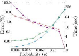
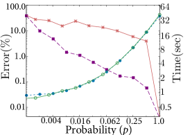
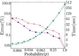
The parameter $p$ controls the probability of an edge being included in the sparsified graph. As $p$ increases, we expect the accuracy as well as the runtime to increase. The relative accuracies of the two methods depends on the variances of the estimators. We estimated the variances using our analysis, and Table 4 presents the results. We observe that the variance of ESpar is predicted to be much lower than that of ClrSpar. To understand this, we begin with Lemmas 15 and 16 which show expressions bounding the variances in terms of $p_{1w},p_{1e},$ and $p_{2v}$, also summarized in Table 4. The difference in the variance between ClrSpar  and ESpar  boils down to $(\mathbin{\mathchoice{\vbox{\hbox{\hskip 1.29167pt\begin{picture}(1.0,1.0)\roundcap\put(0.0,0.27){\line(1,0){1.0}} \put(1.0,0.27){\line(-1,1){1.0}} \put(0.0,1.27){\line(1,0){1.0}} \put(0.0,0.27){\line(1,1){1.0}} \end{picture}\hskip 1.29167pt\vspace{-0.6ex} }}}{\vbox{\hbox{\hskip 1.29167pt\begin{picture}(1.0,1.0)\roundcap\put(0.0,0.27){\line(1,0){1.0}} \put(1.0,0.27){\line(-1,1){1.0}} \put(0.0,1.27){\line(1,0){1.0}} \put(0.0,0.27){\line(1,1){1.0}} \end{picture}\hskip 1.29167pt\vspace{-0.6ex} }}}{\vbox{\hbox{\hskip 1.29167pt\begin{picture}(1.0,1.0)\roundcap\put(0.0,0.27){\line(1,0){1.0}} \put(1.0,0.27){\line(-1,1){1.0}} \put(0.0,1.27){\line(1,0){1.0}} \put(0.0,0.27){\line(1,1){1.0}} \end{picture}\hskip 1.29167pt\vspace{-0.6ex} }}}{\vbox{\hbox{\hskip 1.29167pt\begin{picture}(1.0,1.0)\roundcap\put(0.0,0.27){\line(1,0){1.0}} \put(1.0,0.27){\line(-1,1){1.0}} \put(0.0,1.27){\line(1,0){1.0}} \put(0.0,0.27){\line(1,1){1.0}} \end{picture}\hskip 1.29167pt\vspace{-0.6ex} }}}}{}p^{-3}+p_{2v}p^{-1}-\mathbin{\mathchoice{\vbox{\hbox{\hskip 1.29167pt\begin{picture}(1.0,1.0)\roundcap\put(0.0,0.27){\line(1,0){1.0}} \put(1.0,0.27){\line(-1,1){1.0}} \put(0.0,1.27){\line(1,0){1.0}} \put(0.0,0.27){\line(1,1){1.0}} \end{picture}\hskip 1.29167pt\vspace{-0.6ex} }}}{\vbox{\hbox{\hskip 1.29167pt\begin{picture}(1.0,1.0)\roundcap\put(0.0,0.27){\line(1,0){1.0}} \put(1.0,0.27){\line(-1,1){1.0}} \put(0.0,1.27){\line(1,0){1.0}} \put(0.0,0.27){\line(1,1){1.0}} \end{picture}\hskip 1.29167pt\vspace{-0.6ex} }}}{\vbox{\hbox{\hskip 1.29167pt\begin{picture}(1.0,1.0)\roundcap\put(0.0,0.27){\line(1,0){1.0}} \put(1.0,0.27){\line(-1,1){1.0}} \put(0.0,1.27){\line(1,0){1.0}} \put(0.0,0.27){\line(1,1){1.0}} \end{picture}\hskip 1.29167pt\vspace{-0.6ex} }}}{\vbox{\hbox{\hskip 1.29167pt\begin{picture}(1.0,1.0)\roundcap\put(0.0,0.27){\line(1,0){1.0}} \put(1.0,0.27){\line(-1,1){1.0}} \put(0.0,1.27){\line(1,0){1.0}} \put(0.0,0.27){\line(1,1){1.0}} \end{picture}\hskip 1.29167pt\vspace{-0.6ex} }}}}{}p^{-4})$. In our experiments, we found that $p_{2v}$, the number of pairs of butterflies that share two vertices without sharing an edge, was very high, much larger than $p_{1e}$, $p_{1w}$, and $\mathbin{\mathchoice{\vbox{\hbox{\hskip 1.29167pt\begin{picture}(1.0,1.0)\roundcap\put(0.0,0.27){\line(1,0){1.0}} \put(1.0,0.27){\line(-1,1){1.0}} \put(0.0,1.27){\line(1,0){1.0}} \put(0.0,0.27){\line(1,1){1.0}} \end{picture}\hskip 1.29167pt\vspace{-0.6ex} }}}{\vbox{\hbox{\hskip 1.29167pt\begin{picture}(1.0,1.0)\roundcap\put(0.0,0.27){\line(1,0){1.0}} \put(1.0,0.27){\line(-1,1){1.0}} \put(0.0,1.27){\line(1,0){1.0}} \put(0.0,0.27){\line(1,1){1.0}} \end{picture}\hskip 1.29167pt\vspace{-0.6ex} }}}{\vbox{\hbox{\hskip 1.29167pt\begin{picture}(1.0,1.0)\roundcap\put(0.0,0.27){\line(1,0){1.0}} \put(1.0,0.27){\line(-1,1){1.0}} \put(0.0,1.27){\line(1,0){1.0}} \put(0.0,0.27){\line(1,1){1.0}} \end{picture}\hskip 1.29167pt\vspace{-0.6ex} }}}{\vbox{\hbox{\hskip 1.29167pt\begin{picture}(1.0,1.0)\roundcap\put(0.0,0.27){\line(1,0){1.0}} \put(1.0,0.27){\line(-1,1){1.0}} \put(0.0,1.27){\line(1,0){1.0}} \put(0.0,0.27){\line(1,1){1.0}} \end{picture}\hskip 1.29167pt\vspace{-0.6ex} }}}}$. This explains why the variance of ESpar was higher.

This observation about variance is consistent with our experimental results. In Figure 6, we report the relative percent error as well as the runtime as the sampling probability $p$ increases. Results show that ESpar obtains less than one percent error when $5$ percent of edges are sampled. However, as shown in Figures 6b, 6d and 6e, ClrSpar requires a larger sampling probability to achieve a reasonable accuracy.

	ESamp (with Fast-eBFC)	ESpar
Deli	$3.4$	$2.1$
Journal	$5.0$	$1.7$
Orkut	$3.4$	$3.4$
Web	$4.1$	$3.9$
Wiki-en	$4.8$	$2.3$

Table 5: Time (in seconds) to obtain 1% relative percent error for the best sampling and sparsification algorithms.

6.4 Sampling or Sparsification?

The accuracy of the best sampling algorithm, ESamp with Fast-eBFC, is compared with the best sparsification algorithm, ESpar, in Table 5. Overall, two algorithms take similar times to reach a 1% error on all graphs we considered, in the range of 1.7-5 sec, with ESpar achieving this accuracy faster than ESamp with Fast-eBFC.

However, ESpar has other downsides when compared with ESamp. First, the memory consumption of ESpar is $O(mp)$ where $p$ is a parameter, and is larger than ESamp with Fast-eBFC, whose memory consumption is $O(\Delta)$. As a result, we expect the memory of ESpar to be linearly in the size of the graph, showing that it may be easier for ESamp to scale to graphs of even larger sizes. Next, ESpar needs to decide on a sampling parameter $p$ to balance between accuracy and runtime. If $p$ is too large, then the runtime is high, and if $p$ is too small, then the accuracy is low. Finally, one-shot sparsification algorithms assume that the entire graph is available whereas the ESamp needs access to only a subgraph of the graph. Thus if one has to pay for data about the graph, or if the data about edges is hard to obtain, then sampling may be the better alternative.

Overall, local sampling algorithms can find a larger application space in real-world. If the entire graph is available, and memory is not a bottleneck, it may be better to go with ESpar. For more restrictive scenarios, ESamp combined with Fast-eBFC is the better option.

7 Conclusion

We introduced a suite of algorithms for butterfly counting in bipartite networks. We first showed that a simple statistic about vertex sets, which is cheap to obtain, helps drastically to reduce the runtime of exact algorithms. We then presented scalable randomized algorithms that approximate the number of butterflies in a graph, with provable accuracy guarantees.

Randomized algorithms using one-shot sparsification are applicable when the entire graph is available locally, and rely on a global sampling step to compute a smaller “sparsified” subgraph, which is used to compute an accurate estimate. On the other hand, if the access to the graph data is limited, local sampling algorithms can be used to randomly sample small subgraphs of the entire graph, and analyze them to compute an estimate. Sampling algorithms are especially beneficial when there is a rate-limited API that provides random samples of the network data, such as the GNIP gni (2017) and Facebook Graph API fbg (2017). Our best sampling and sparsification algorithms yield less than $1\%$ relative error within $\approx 5$ and $\approx 4$ seconds for all the networks we considered, whereas the state-of-the-art exact algorithm does not complete even in 40,000 secs on the Web graph.

There are many promising directions to follow. Here we only focused on the butterfly motif, but one can consider other motifs suitable to bipartite graphs. Note that the combinatorial explosion for the number of butterflies is more serious than the triangles in unipartite graphs. Thus it is challenging to consider even larger motifs, but the ideas in this work can serve as building blocks for considering different motifs. Another direction is adapting our algorithms for the streaming scenario. Given a single pass over the graph, the question is how to sample/sparsify the graph stream to accurately estimate the number of butterflies. Sparsification-based algorithms may be adapted to the streaming scenario quite easily, but same cannot be said for the local sampling algorithms.

References

- [1]
- gni [2017] 2017. GNIP. (2017). (https://gnip.com/about/ ).
- fbg [2017] 2017. The Graph API for the Facebook Social Graph. (2017). (https://developers.facebook.com/docs/graph-api).
- Ahmed et al. [2016] N. K. Ahmed, J. Neville, R. A. Rossi, N. Duffield, and T. L. Willke. 2016. Graphlet Decomposition: Framework, Algorithms, and Applications. KAIS (2016), 1–32.
- Aksoy et al. [2017] S. Aksoy, T. G. Kolda, and A. Pinar. 2017. Measuring and Modeling Bipartite Graphs with Community Structure. Journal of Complex Networks 5, 4 (2017), 581–603.
- Alon et al. [1997] N. Alon, R. Yuster, and U. Zwick. 1997. Finding and counting given length cycles. Algorithmica 17, 3 (1997), 209–223.
- Borgatti and Everett [1997] Stephen P. Borgatti and Martin G. Everett. 1997. Network analysis of 2-mode data. Social Networks 19, 3 (1997), 243 – 269.
- Bressan et al. [2017] Marco Bressan, Flavio Chierichetti, Ravi Kumar, Stefano Leucci, and Alessandro Panconesi. 2017. Counting Graphlets: Space vs Time. In WSDM. 557–566.
- De Stefani et al. [2016] L. De Stefani, A. Epasto, M. Riondato, and E. Upfal. 2016. TRIÈST: Counting Local and Global Triangles in Fully-Dynamic Streams with Fixed Memory Size. In KDD. 825–834.
- Halford and Chugg [2006] T. R. Halford and K. M. Chugg. 2006. An algorithm for counting short cycles in bipartite graphs. IEEE Transactions on Information Theory 52, 1 (2006), 287–292.
- Itai and Rodeh [1978] Alon Itai and Michael Rodeh. 1978. Finding a Minimum Circuit in a Graph. SIAM J. Comput. 7, 4 (1978), 413–423.
- Jain and Seshadhri [2017] Shweta Jain and C. Seshadhri. 2017. A Fast and Provable Method for Estimating Clique Counts Using Turán’s Theorem. In WWW. 441–449.
- Jha et al. [2015] Madhav Jha, C. Seshadhri, and Ali Pinar. 2015. Path Sampling: A Fast and Provable Method for Estimating 4-Vertex Subgraph Counts. In WWW. 495–505.
- Latapy et al. [2008] M. Latapy, C. Magnien, and N. Del Vecchio. 2008. Basic notions for the analysis of large two-mode networks. Social Networks 30, 1 (2008), 31 – 48.
- Lim and Kang [2015] Yongsub Lim and U Kang. 2015. MASCOT: Memory-efficient and Accurate Sampling for Counting Local Triangles in Graph Streams. In KDD. 685–694.
- Lind et al. [2005] Pedro G. Lind, Marta C. González, and Hans J. Herrmann. 2005. Cycles and clustering in bipartite networks. Phys. Rev. E 72 (2005), 056127. Issue 5.
- Milo et al. [2002] R. Milo, S. Shen-Orr, S. Itzkovitz, N. Kashtan, D. Chklovskii, and U. Alon. 2002. Network Motifs: Simple Building Blocks of Complex Networks. Science 298, 5594 (2002), 824–827.
- Newman [2001a] M.E.J. Newman. 2001a. Scientific collaboration networks. II. Shortest paths, weighted networks, and centrality. Phys. Rev. E 64 (2001), 016132. Issue 1.
- Newman [2001b] M. E. J. Newman. 2001b. Scientific collaboration networks. I. Network construction and fundamental results. Phys. Rev. E 64 (2001), 016131. Issue 1.
- Opsahl [2013] Tore Opsahl. 2013. Triadic closure in two-mode networks: Redefining the global and local clustering coefficients. Social Networks 35, 2 (2013), 159 – 167. Special Issue on Advances in Two-mode Social Networks.
- Pagh and Tsourakakis [2012] Rasmus Pagh and Charalampos E Tsourakakis. 2012. Colorful triangle counting and a mapreduce implementation. Inform. Process. Lett. 112, 7 (2012), 277–281.
- Pavan et al. [2013] A. Pavan, K. Tangwongsan, S. Tirthapura, and K. Wu. 2013. Counting and Sampling Triangles from a Graph Stream. PVLDB 6, 14 (2013), 1870–1881.
- Pinar et al. [2017] Ali Pinar, C. Seshadhri, and Vaidyanathan Vishal. 2017. ESCAPE: Efficiently Counting All 5-Vertex Subgraphs. In WWW. 1431–1440.
- Robins and Alexander [2004] Garry Robins and Malcolm Alexander. 2004. Small Worlds Among Interlocking Directors: Network Structure and Distance in Bipartite Graphs. Computational & Mathematical Organization Theory 10, 1 (2004), 69–94.
- Sanei-Mehri et al. [2018] S.-V. Sanei-Mehri, A. Erdem Sariyuce, and S. Tirthapura. 2018. Butterfly Counting in Bipartite Networks. ArXiv e-prints (Dec. 2018). arXiv:1801.00338
- Sarıyüce and Pinar [2018] Ahmet Erdem Sarıyüce and Ali Pinar. 2018. Peeling Bipartite Networks for Dense Subgraph Discovery. In WSDM.
- Seshadhri et al. [2014] C. Seshadhri, A. Pinar, and T. G. Kolda. 2014. Triadic Measures on Graphs: The Power of Wedge Sampling. Statistical Analysis and Data Mining 7, 4 (2014), 294–307.
- Tangwongsan et al. [2013] K. Tangwongsan, A. Pavan, and S. Tirthapura. 2013. Parallel Triangle counting in massive streaming graphs. In CIKM. 781–786.
- Tsourakakis et al. [2009] Charalampos E Tsourakakis, U Kang, Gary L Miller, and Christos Faloutsos. 2009. Doulion: counting triangles in massive graphs with a coin. In KDD. 837–846.
- Turkoglu and Turk [2017] D. Turkoglu and A. Turk. 2017. Edge-Based Wedge Sampling to Estimate Triangle Counts in Very Large Graphs. In 2017 IEEE ICDM. 455–464.
- Wang et al. [2014] J. Wang, A. W. C. Fu, and J. Cheng. 2014. Rectangle Counting in Large Bipartite Graphs. In 2014 IEEE International Congress on Big Data. 17–24.
- Wu et al. [2016] B. Wu, K. Yi, and Z. Li. 2016. Counting Triangles in Large Graphs by Random Sampling. IEEE TKDE 28, 8 (2016), 2013–2026.