Dark-dark-soliton dynamics in two density-coupled Bose-Einstein condensates

Abstract

We study the 1D dynamics of dark-dark solitons in the miscible regime of two density-coupled Bose-Einstein condensates having repulsive interparticle interactions within each condensate ($g>0$). By using an adiabatic perturbation theory in the parameter $g_{12}/{g}$, we show that, contrary to the case of two solitons in scalar condensates, the interactions between solitons are attractive when the interparticle interactions between condensates are repulsive $g_{12}>0$. As a result, the relative motion of dark solitons with equal chemical potential $\mu$ is well approximated by harmonic oscillations of angular frequency $w_{r}=(\mu/\hbar)\sqrt{({8}/{15}){g_{12}}/{g}}$. We also show that in finite systems, the resonance of this anomalous excitation mode with the spin density mode of lowest energy gives rise to alternating dynamical instability and stability fringes as a function of the perturbative parameter. In the presence of harmonic trapping (with angular frequency $\Omega$) the solitons are driven by the superposition of two harmonic motions at a frequency given by $w^{2}=(\Omega/\sqrt{2})^{2}+w_{r}^{2}$. When $g_{12}<0$, these two oscillators compete to give rise to an overall effective potential that can be either single well or double well through a pitchfork bifurcation. All our theoretical results are compared with numerical solutions of the Gross-Pitaevskii equation for the dynamics and the Bogoliubov equations for the linear stability. A good agreement is found between them.

I Introduction

Over the last two decades, Bose-Einstein condensation (BEC) has enabled the study of numerous physical concepts Pitaevskii2003 ; Pethick2008 . Among them, an interesting scenario is the connection between the non-linear waves and atomic systems, that leads to the so-called matter-wave solitons Kevrekidis2008 ; Kevrekidis2015 . These structures emerge from the balance between linear dispersion and interactions, which are accounted for from non-linear terms in the equations of motion. Specifically, mean field descriptions of BECs, as provided by the Gross-Pitaevskii equation (GP), incorporate a non-linear term proportional to the interatomic interaction strength $g$, which is measured by the s-wave scattering length $a$. Depending on the sign and magnitude of the latter and the dimensionality of the system, a large number of structures can be found: dark Frantzeskakis2010 and bright Strecker2003 solitons, vortices Fetter2001 , etc.

Dark solitons in BECs are localized non-linear excitations that present a notch in the condensate density and a phase step across its center. They have been observed in numerous experiments using different techniques Burger1999 ; Becker2008 ; Weller2008 ; Lamporesi2013 ; Anderson1999 and this has inspired a large number of theoretical works (see Frantzeskakis2010 and references therein). Specifically, the problem of dark solitons in BECs confined by parabolic external traps has been extensively studied William1997 ; Muryshev1999 ; Busch2000 ; Pelinovsky2005 .

Another interesting aspect of BECs is the study of multi-component systems, which can be described by a set of coupled GP equations. These systems were soon realized in ultracold-gas experiments by coupling two condensates made of either different atomic species Cornell1998 or different hyperfine states of the same atomic species Myatt1997 . This fact inspired the study of matter-wave solitons in these settings, and new families of solitonic structures have been found: dark-dark Ohberg2001 ; Hoefer2011 ; Yan2012 , dark-bright Middelkamp2011 ; Yan2011 ; Achilleos2011 , dark-antidark Danaila2016 , etc. Particular attention has been given to the so-called Manakov limit in 1D settings, where the intra- and inter-condensate particle interactions match Yan2012 .

The aim of this work is to study the dynamics of dark-dark solitons in a one-dimensional setting of two density-coupled condensates out of the Manakov limit, for varying coupling between condensates. Specifically, we consider a mean-field description of BECs composed by two hyperfine states of the same alkali species, and inspect both the case without any axial trap, termed untrapped, and the case with a harmonic trap in the axial direction. Within the Hamiltonian approach of the perturbation theory for solitons Uzunov1993 ; Kivshar1994 ; Frantzeskakis2002 , we obtain analytical expressions for the adiabatic evolution of the dark-dark soliton. For the untrapped case we find that when the interaction between components is repulsive the dark-dark soliton can be seen as a bound state of two dark solitons performing a relative harmonic motion. For attractive interactions such a bound state can not exist because the dark solitons repel each other. An equivalent study is also performed for the confined case, where the competition between soliton interactions and harmonic trapping is found to produce sizable changes on the dynamics, leading for example to bound states even with attractive interactions. Our analytical results are tested with different numerical techniques: direct simulations of the Gross-Pitaevskii equations, Fourier analysis to extract characteristic frequencies of the motion, and numerical solution of the Bogoliubov equations for the linear excitations of stationary states. In what follows, we first introduce the theoretical model in section II, and next we show our numerical results in section III. To sum up, we present our conclusions in section IV.

II Theoretical model

The dynamics of a BEC at zero temperature can be accurately described within the mean field approach in terms of a wave-function $\psi(\mathbf{r},t)$. In a one dimensional setting, the wave functions of two trapped, density-coupled BECs are governed by corresponding Gross-Pitaevskii equations

$$\begin{aligned} &i\hbar\frac{\partial}{\partial t}\psi_{1}=\left(\frac{-\hbar^{2}}{2m}\frac{\partial^{2}}{\partial z^{2}}+\frac{m\Omega_{z}^{2}z^{2}}{2}+g|\psi_{1}|^{2}+g_{12}|\psi_{2}|^{2}\right)\psi_{1}\\ &i\hbar\frac{\partial}{\partial t}\psi_{2}=\left(\frac{-\hbar^{2}}{2m}\frac{\partial^{2}}{\partial z^{2}}+\frac{m\Omega_{z}^{2}z^{2}}{2}+g|\psi_{2}|^{2}+g_{12}|\psi_{1}|^{2}\right)\psi_{2}\,,\end{aligned}$$ (1)

where $\Omega_{z}$ is the angular frequency of the axial harmonic trapping, $g=2\hbar\Omega_{\perp}a$ is the reduced 1D strength of the interaction between particles of the same condensate, which is proportional to the energy of the transverse trapping $\hbar\Omega_{\perp}$ and to the scattering length $a$, and $g_{12}=2\hbar\Omega_{\perp}a_{12}$ is the strength of the density coupling between condensates, proportional to the scattering length between particles of different condensates $a_{12}$.

A stationary soliton solution to Eq. (1) $\psi_{i}(z,t)$, with $i=1,2$, can be written as the product of a time-independent (and real function) background component $\phi_{i}$ and the soliton excitation $v_{i}$, so that

$$\psi_{i}(z,t)=\phi_{i}(z)v_{i}(z,t)e^{-i\mu_{i}t/\hbar},$$ (2)

where $\mu_{i}$ is the chemical potential. It is important to remark that both $\psi_{i}$ and $\phi_{i}$ satisfy the coupled GP equations for the same chemical potential:

$$\mu_{i}\phi_{i}=\left(-\frac{1}{2}\frac{\partial^{2}}{\partial z^{2}}+\frac{1}{2}\Omega^{2}z^{2}+g\phi_{i}^{2}+g_{12}\phi_{j}^{2}\right)\phi_{i}$$ (3)

$$i\frac{\partial}{\partial t}\psi_{i}=\left(-\frac{1}{2}\frac{\partial^{2}}{\partial z^{2}}+\frac{1}{2}\Omega^{2}z^{2}+g|\psi_{i}|^{2}+g_{12}|\psi_{j}|^{2}\right)\psi_{i}\,,$$ (4)

where $\Omega=\Omega_{z}/\Omega_{\perp}$ is the trap aspect ratio, and we have written the equations in dimensionless form by using transverse trap units, $a_{\perp}=\sqrt{\hbar/m\Omega_{\perp}}$ as unit length and $t_{\perp}=\Omega_{\perp}^{-1}$ as unit time, and for the sake of a simple notation have kept the same letters for the dimensionless couplings ${g}$ and ${g}_{12}$. So, from Eqs. (3)-(4) we can obtain corresponding equations for the soliton wave functions $v_{i}(z,t)$

$$\left(i\frac{\partial}{\partial t}+\frac{1}{2}\frac{\partial^{2}}{\partial z^{2}}-g\phi^{2}_{i}\left(|v_{i}|^{2}-1\right)-g_{12}\phi^{2}_{j}\left(|v_{j}|^{2}-1\right)\right)v_{i}=$$

$$\hskip 14.22636pt=-\frac{\partial v_{i}}{\partial z}\,\frac{\partial\ln\phi_{i}}{\partial z}\,,$$ (5)

where the external trap does not appear explicitly, although its information is encoded in the background wavefunctions $\phi_{i}$.

II.1 Untrapped case

Here we set $\Omega=0$, hence the ground state solutions to Eq. (3) are the constant density $|\phi_{i}|^{2}=n_{i}$ states

$$n_{i}=\frac{g\mu_{i}-g_{12}\mu_{j}}{g^{2}-g^{2}_{12}}.$$ (6)

The equations of motion for soliton states Eq. (5) can be written as

$$\left(i\frac{\partial}{\partial t}+\frac{1}{2}\frac{\partial^{2}}{\partial z^{2}}-g\,n_{i}\,\left(|v_{i}|^{2}-1\right)-g_{12}\,n_{j}\,\left(|v_{j}|^{2}-1\right)\right)v_{i}=0.$$ (7)

As we said before, we are going to deal with the coupling between condensates in a perturbative way. Then, assuming that $g_{12}<<g$, the background densities Eq. (6) become $n_{i}\approx\mu_{i}/g-(g_{12}/g)\,\mu_{j}/g$, and neglecting terms proportional to $g_{12}^{2}$ in Eq. (7) we get

$$\begin{aligned} &i\frac{\partial v_{i}}{\partial t}+\frac{1}{2}\frac{\partial^{2}v_{i}}{\partial z^{2}}-\mu_{i}\left(|v_{i}|^{2}-1\right)v_{i}=\\ &=-\frac{g_{12}}{g}\mu_{j}\left(|v_{i}|^{2}-|v_{j}|^{2}\right)v_{i}\equiv\frac{g_{12}}{g}\mu_{j}P(v_{i},v_{j}).\end{aligned}$$ (8)

On the left hand side of this equality we have the well known non-linear Schrödinger equation for the wave function $v_{i}$, whereas on the right hand side we get a perturbative term in the parameter $g_{12}/g$. In order to obtain analytical expressions for the interactions between solitons, from now on we will focus on the case of equal backgrounds $\phi_{1}=\phi_{2}=\phi$, and then $\mu_{1}=\mu_{2}=\mu=(g+g_{12})n$. So that, by dividing the whole equation (8) by $\mu$, we set new units for space $\hbar/\sqrt{m\mu}$ and time $\hbar/\mu$. In these units we introduce the general dark soliton solution

$$\begin{aligned} &v_{i}(z,t)=\cos\varphi_{i}\tanh\zeta_{i}+i\sin\varphi_{i},\end{aligned}$$ (9)

where $\zeta_{i}=\cos\varphi_{i}(z-t\sin\varphi_{i})$, and $\varphi_{i}$ parametrizes the soliton darkness, that is $|v_{i}|^{2}=(1-\cos^{2}\varphi_{i}\,\mbox{sech}^{2}\,\zeta_{i})$, and the soliton velocity $\dot{z}_{0}=\sin\varphi_{i}$, that is the time derivative of the soliton position $z_{0}$, taken at minimum density.

In the absence of perturbation, $P(v_{i},v_{j})=0$, the solution Eq. (9) describes overlapping solitons moving at constant velocity, and hence $\ddot{z}_{0}=\dot{\varphi}_{i}=0$. However, the effect of the perturbation $P(v_{i},v_{j})$ leads to the adiabatic time evolution of the soliton parameters, $(\varphi,z_{0})\rightarrow(\varphi(t),z_{0}(t))$. This evolution can be described by the equation Kivshar1994

$$\dot{\varphi}_{i}=\frac{g_{12}/g}{2\cos^{2}\varphi_{i}\sin\varphi_{i}}\Re\left[\int_{-\infty}^{\infty}P(v_{i},v_{j})\frac{\partial v_{i}^{*}}{\partial t}dz\right].$$ (10)

Assuming solitons with high density depletions $\varphi_{i}<<1$ and separated by a relative distance $2z_{0}$, such that $\zeta_{1}=\cos\varphi_{1}\left(z-z_{0}\right)$ and $\zeta_{2}=\cos\varphi_{2}\left(z+z_{0}\right)$, Eq. (10) gives

$$\dot{\varphi}_{1}=-\frac{g_{12}}{g}f(z_{0})\equiv\,F_{\rm eff}^{(i)}(z_{0}),$$ (11)

where $f(z_{0})=8\sinh(2z_{0})e^{6z_{0}}(3-3e^{8z_{0}}+(1+4e^{4z_{0}}+e^{8z_{0}})4z_{0})/(e^{4z_{0}}-1)^{5}$. As can be seen, for $z_{0}=0$, that is for overlapped solitons, $\dot{\varphi}_{1}=0$ and the solitons evolve without relative motion. Since, in this limit ($\varphi<<1$) $\dot{z}_{0}\approx\varphi$, Eq. (11) is also an equation for $\ddot{z}_{0}$, with the right hand side playing the role of a classical force $F_{\rm eff}^{(i)}(z_{0})$ derived from an effective potential $U_{\rm eff}^{(i)}(z_{0})$ :

$$\ddot{z}_{0}=-\frac{dU_{\rm eff}^{(i)}(z_{0})}{dz_{0}}.$$ (12)

This potential accounts for the interactions between the solitons and is the source of their relative motion. After integration of the force Eq. (11) over $z_{0}$, we get

$$U_{\rm eff}^{(i)}(z_{0})=\frac{g_{12}}{g}\,\frac{2(1+e^{4z_{0}})(1-2z_{0})-4}{e^{-4z_{0}}\,(e^{4z_{0}}-1)^{3}}.$$ (13)

As it has been anticipated, it presents a minimum at $z_{0}=0$, allowing for the existence of a bound state made of overlapped solitons, and tends exponentially to zero for finite values of the inter-soliton distance $2z_{0}$ (see Fig. 1). For small separation $z_{0}\rightarrow 0$, the Taylor expansion reads

$$U_{\rm eff}^{(i)}(z_{0})\sim\frac{g_{12}}{g}\left(-\frac{1}{6}+\frac{4}{15}z^{2}_{0}\right)+O[z^{4}_{0}]\,,$$ (14)

Figure 1: Top panel: Effective force experienced by a dark soliton forming a dark-dark soliton system for $g_{12}/g=0.01$ in the absence of trapping. Bottom panel: Soliton interaction potential Eq. (13) from which the above effective force is derived. The solitons oscillate in a relative motion around the minimum at $z_{0}=0$.

and the equation of relative motion Eq. (12) simplifies to that of a harmonic oscillator, $\ddot{z}_{0}+w_{r}^{2}\,z_{0}=0$, with angular frequency (for generic chemical potential $\mu$)

$$w_{r}=\mu\sqrt{\frac{8}{15}\frac{g_{12}}{g}}.$$ (15)

This is the frequency of small oscillations of the two solitons around their center of mass, moving at constant velocity $v_{CM}=(\sin\varphi_{1}+\sin\varphi_{2})/2$. It is also interesting to note that this model predicts an instability (imaginary frequency) when $g_{12}<0$, due to the fact that the effective potential $U_{\rm eff}^{(i)}$ presents a maximum for attractive interparticle interactions between particles of different condensates, and as a consequence, it prevents the existence of a bound solitonic state in this case.

II.2 Trapped case

In the presence of axial harmonic trapping $V(z)=\frac{1}{2}\Omega^{2}z^{2}$, we rely on the Thomas-Fermi (TF) approximation to study the strong (interparticle) interacting regime ($\mu_{i}>>\Omega$) Pitaevskii2003 . There the inhomogeneous ground state densities, $n_{i}(z)=|\phi_{i}|^{2}$, are given by

$$n_{i}(z)=\frac{g\mu_{i}(z)-g_{12}\mu_{j}(z)}{g^{2}-g^{2}_{12}},$$ (16)

where $\mu_{i}(z)=\mu_{i}-V(z)$ are the local chemical potentials. In the limit of $g_{12}<<g$, we get

$$g\,n_{i}(z)={\mu_{i}(z)}-\frac{g_{12}}{g}{\mu_{j}(z)},$$ (17)

and, as a result, the equations of motion for soliton solutions Eq. (5) become

$$i\frac{\partial v_{i}}{\partial t}+\frac{1}{2}\frac{\partial^{2}v_{i}}{\partial z^{2}}-\mu_{i}(z)\left(|v_{i}|^{2}-1\right)v_{i}=$$

$$=-\frac{g_{12}}{g}\mu_{j}(z)\left(|v_{i}|^{2}-|v_{j}|^{2}\right)v_{i}-\frac{\partial v_{i}}{\partial z}\,\frac{d\ln\phi_{i}}{dz}.$$ (18)

The local chemical potentials and the last term in the right hand side of this equation are the main differences with respect to the untrapped case Eq. (8). In spite of these differences, and due to the fact that the background densities change slowly inside the TF regime ($dV/dz\rightarrow 0$), an analogue perturbative approach can still be followed, and the governing equation for the dark soliton $v_{i}$ is

$$i\frac{\partial v_{i}}{\partial t}+\frac{1}{2}\frac{\partial^{2}v_{i}}{\partial z^{2}}-\mu_{i}(z)v_{i}\left(|v_{i}|^{2}-1\right)=P(v_{i},v_{j};V(z)),$$ (19)

where the perturbation $P(v_{i},v_{j};V)$ is given by

$$P(v_{i},v_{j};V)\approx-\frac{g_{12}}{g}\mu_{j}(z)\left(|v_{i}|^{2}-|v_{j}|^{2}\right)v_{i}+$$

$$\hskip 14.22636pt+\frac{1}{2\mu(z)}\frac{dV}{dz}\frac{\partial v_{i}}{\partial z},$$ (20)

which, along with the term associated to the interaction between dark solitons, contains a new term introduced by the external trap Frantzeskakis2010 .

Again, we focus on the symmetric case $\mu_{1}=\mu_{2}=\mu$, where the local chemical potential reads $\mu(z)=\mu-V(z)=(g+g_{12})\,n(z)$. In the particular case of motion around the center of the harmonic potential $\mu(z)\rightarrow\mu$, and by following the same procedure as in the untrapped case (with $\hbar/\sqrt{m\mu}$ and $\hbar/\mu$ as space and time units respectively) we can obtain a particle-like evolution for the soliton position $z_{0}$

Figure 2: (Color online) Forces (top panel) and total, single-well potential (bottom panel) experienced by each dark soliton forming a dark-dark soliton system with $\mu=1$ and $g_{12}>0$ in the presence of a harmonic trap with $\Omega=0.1$. The dashed (red) line represents the force caused by the trap, whereas the continuous lines represent the effective force due to the interaction with the other dark soliton.

$$\ddot{z}_{0}=-\frac{\Omega^{2}}{2\mu^{2}}z_{0}-F_{\rm eff}^{(i)},$$ (21)

where the right hand side is the total effective force acting on the soliton $F_{\rm eff}=-dU_{\rm eff}/d\,z_{0}$, and embraces the superposition of the action of the external trap and the soliton interaction. For small-amplitude oscillations $z_{0}\approx 0$, we get

$$\ddot{z}_{0}=-\left(\frac{\Omega^{2}}{2\mu^{2}}+\frac{8}{15}\frac{g_{12}}{g}\right)z_{0}+\frac{64}{63}\frac{g_{12}}{g}z_{0}^{3}+O(z_{0}^{5}),$$ (22)

where the balance between the two harmonic force terms (inside the parenthesis) leads to different scenarios depending on the sign of the coupling interaction $g_{12}$.

Figure 3: (Color online) Same as Fig. 2 for $g_{12}<0$. Three cases are depicted for different $g_{12}/g$ values, below (blue), at (orange) and above (green) the threshold $g_{c}$ indicating the change in the shape of the total effective potential from single well $g_{12}/g<c_{c}$ to double well $g_{12}/g>g_{c}$ (see text).

II.2.1 Repulsive coupling: ${g_{12}>0}$

Figure 2 shows the effective force and effective potential defined in Eq. (21) for varying values of $g_{12}/g$ at a given trapping $\Omega=0.1$. As can be seen, the different parameters do not produce qualitative changes in the potential, which presents a single minimum capable to bound the coupled solitons. As in the untrapped case, our theory predicts that the dark solitons will perform small-amplitude oscillations around $z_{0}=0$ with angular frequency (in transverse oscillator units)

$$w=\left(\frac{\Omega^{2}}{2}+\frac{8}{15}\frac{g_{12}}{g}\mu^{2}\right)^{\frac{1}{2}}.$$ (23)

As we will see later, our numerical results demonstrate that the minimum supports a bound state that exists and is stable for small $g_{12}/g$. However, for increasing values of this parameter both stable and unstable cases can be found depending on the particular valued of the chemical potential of the system.

II.2.2 Attractive coupling: ${g_{12}<0}$

The phenomenology is richer for attractive interactions between particles of different condensates. In contrast to the untrapped case, the presence of the harmonic potential allows for the generation of local minima in the total effective potential that can support stationary states made of two solitons. As shown in Fig. 3, by increasing the parameter $|g_{12}/g|$, the total effective potential modifies from a single well (an also a unique fixed point $z_{0}^{*}=0$ in the equation of motion) to a double well potential (with three fixed points). Specifically, the system shows a pitchfork bifurcation at $g_{c}=|g_{12}/g|={15}(\Omega/\mu)^{2}/16$, hence for $|g_{12}/g|>g_{c}$ the fixed point at $z_{0}^{*}=0$ loses its stability and two new off-center, stable fixed points appear. From Eq. (22) we get their position at

$$z_{0_{\pm}}^{*}=\pm\frac{1}{\sqrt{\mu}}\sqrt{\frac{21}{40}-\frac{63}{128}\left|\frac{g}{g_{12}}\right|\left(\frac{\Omega}{\mu}\right)^{2}}.$$ (24)

Figure 4: (Color online) Stationary state made of two solitons situated at the fixed points $z_{0_{\pm}}^{*}$ of the effective potential (see text) for $\mu=10\,\Omega$ and $g_{12}/g=-0.1$.

As can be noted, the separation between minima increases with $\mu/\,\Omega$ for given $g_{12}/g$, and saturates at a distance of $2z_{0}^{*}=1.44$. Fig. 4 shows an example of a stationary state with two separated solitons occupying the two minima of the effective potential at $\mu=10\,\Omega$ and $g_{12}/g=-0.1<g_{c}$.

For small distances $\epsilon(t)$ around the fixed points $z_{0_{\pm}}^{*}$, from the substitution of $z_{0}(t)=z_{0}^{*}+\epsilon(t)$ in Eq. (22), the solitons oscillate according to

$$\ddot{\epsilon}=-\left(w_{1}(z_{0_{\pm}}^{*})^{2}+w^{2}\right)\epsilon\equiv-w_{\rm eff}^{2}\epsilon,$$ (25)

up to linear terms in the perturbation $\epsilon(t)$, where $w$ is the angular frequency given by (23), and $w_{1}(z_{0})^{2}=-2f(z_{0})\left(\mbox{sech}(z_{0})-{5}/{\sinh(2z_{0})}+3\right)-$ $\left(\left(1+4e^{4z_{0}}+e^{8z_{0}}\right)+\left(-12e^{8z_{0}}+\left(16e^{4z_{0}}+8e^{8z_{0}}\right)z_{0}\right)\right)$ $64e^{6z_{0}}/\left(e^{4z_{0}}-1\right)^{5}$.

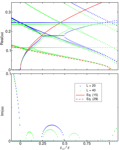
Figure 5: (Color online) Bogoliubov modes in 1D rings of different size (untrapped case). The upper panel depicts the real part of the frequencies and the lower panel the imaginary parts. The solid and dashed lines correspond to Eqs. (15) and (40), respectively, the crossing of which indicates the appearance of instabilities.

III Numerical results

In what follows, in order to test our analytical predictions on the dark-dark-soliton dynamics, we first numerically solve the GP equation to obtain these stationary states for varying chemical potentials and interactions strengths. Afterwards, the soliton stability is monitored both in the nonlinear regime (by simulating the real time evolution with the GP equation) and by linear analysis around the equilibrium states. The latter is performed by solving the Bogoliubov equations for the linear excitations $[u(z,t),v(z,t)]$ around the dark-dark soliton states $\psi(z,t)=\exp(-i\mu t)[\psi(z)+\sum_{\omega}(u\,e^{-i\omega t}+v^{*}e^{i\omega t})]$. These equations are:

$$B\left(\begin{array}[]{c}u_{1}\\ v_{1}\\ u_{2}\\ v_{2}\end{array}\right)=\omega\left(\begin{array}[]{c}u_{1}\\ v_{1}\\ u_{2}\\ v_{2}\end{array}\right),$$ (34)

where:

$$B=\left(\begin{array}[]{cccc}h_{1}&g\psi_{1}^{2}&g_{12}\psi_{1}\psi_{2}^{*}&g_{12}\psi_{1}\psi_{2}\\ -g\psi_{1}^{*2}&-h_{1}&-g_{12}\psi_{1}^{*}\psi_{2}^{*}&-g_{12}\psi_{1}^{*}\psi_{2}\\ g_{12}\psi_{1}^{*}\psi_{2}&g_{12}\psi_{1}\psi_{2}&h_{2}&g\psi_{2}^{2}\\ -g_{12}\psi_{1}^{*}\psi_{2}^{*}&-g_{12}\psi_{1}\psi_{2}^{*}&-g\psi_{2}^{*2}&-h_{2}\end{array}\right).$$ (39)

Here $h_{i}=-\frac{1}{2}\frac{\partial^{2}}{\partial z^{2}}+\frac{1}{2}\Omega^{2}z^{2}+2g|\psi_{i}|^{2}+g_{12}|\psi_{j\neq i}|^{2}-\mu_{i}$. They can be seen as an eigenvalue problem with a non-trivial solution given by ${\rm det}|B-\omega I|=0$.

Apart from the perturbative case $g_{12}<<g$, we also explore numerically the stability of overlapped solitons in the whole miscible regime $g_{12}<g$, and show that the finite size of the system determines the stability properties.

III.1 Untrapped case

Figure 6: (Color online) Spatio-temporal evolution of the density of two untrapped dark-dark solitons with $\mu=1$, $g_{12}=0.015$ and $g=1$ obtained from the numerical solution of the GP Eq. (1). The top and down panel correspond to component 1 and 2 respectively. The continuous (colour) lines represent the evolution of the dark solitons positions given by Eq. (15).

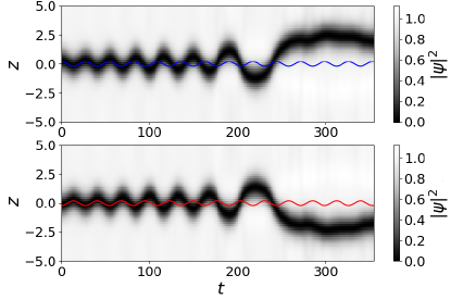
Figure 7: Same as Fig. 6 but with $g_{12}=0.1$.

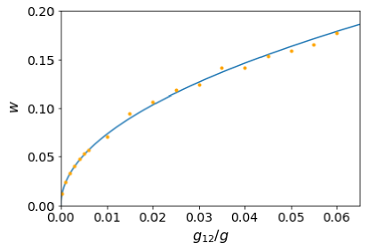
Figure 8: (Color online) Soliton relative motion frequency as a function of the interparticle strength ratio in the absence of external trap. The continuous (blue) line represents our theoretical prediction Eq. (15) and the (orange) dots are values extracted by means of Fourier analysis from the numerical solution of the time dependent GP equation.

The excitation frequencies of the stationary states can be readily extracted by solving the Bogoliubov equations Eq. (34). In the Appendix we analytically show that there are two zero modes of excitation at $g_{12}/g=0$, and $1$, and hence that the system of overlapped dark solitons is expected to be unstable in between. However such analysis assume an infinite system, and the situation is quite different in systems of finite size, where ranges of dynamical stability can be found. Fig. 5 shows two examples of this phenomenon, where the Bogoliubov modes are computed for overlapped solitons with the same chemical potential $\mu=0.5$ in 1D rings of different sizes $L=20,\;40$. The instability emerge from a Hopf bifurcation, which occurs due to the collision of two excitation modes (see the discussion about this collision in the next section): one mode associated to the oscillations around the minimum of the effective potential of soliton interactions, given by expression (15) and represented in Fig. 5 by the solid red curve, and the background spin density mode of lowest energy (represented by the dashed curve for the longer ring), which is given by the analytical expression (in full units) Abad2013 :

$$\hbar\omega=\sqrt{\frac{\hbar^{2}k^{2}}{2m}\left(\frac{\hbar^{2}k^{2}}{2m}+2(g-g_{12})n\right)}.$$ (40)

The small disagreement between the crossing of these analytical curves and the beginning of instabilities in the numerical results arises from the curvature of the modes near the bifurcation point, and decreases for longer rings. This first instability triggers new collisions between modes and, as a consequence, more instability regions. The longer the ring the higher the number of instability regions in the system, approaching the prediction for the infinite case. It is worth remarking that the bound state mode predicted by Eq. (15), in excellent agreement with the numerics, does not change with the size of the ring.

To analyze the dynamics of dark-dark solitons in the bound state allowed by the repulsive interparticle interactions $g_{12}>0$, we excite the relative motion of the solitons by imposing the initial ansatz

$$\begin{aligned} &\psi_{1}=\sqrt{n}\tanh\left(z-z_{0}\right)\\ &\psi_{2}=\sqrt{n}\tanh\left(z+z_{0}\right),\end{aligned}$$ (41)

and we fix $\mu=1$. Figures 6–7 show the comparison between the subsequent motion of the solitons from the numerical solution of GP Eq. (1), and the analytical prediction by Eq. (15) fitted to $y(t)=z_{0}\cos{wt}$. As can be seen, it provides a reasonable good estimate for small $g_{12}$ (Fig. 6) but fails for larger $g_{12}$ (Fig. 7) or also long times.

In order to obtain a more quantitative comparison we have run different real time evolutions for varying $g_{12}$ and equal chemical potential $\mu=1$. By tracking the position of the solitons (at minimum density), we have computed their characteristic frequency from a Fourier analysis in time. The numerical results are presented in Fig. 8, and show a very good agreement with our analytical prediction for small values of $g_{12}/g$.

III.2 Trapped case

III.2.1 Attractive interaction between condensates: ${g_{12}<0}$

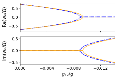
Figure 9: (Color online) Frequency of the dark soliton relative motion in a harmonic trap with $\Omega=0.1$. The real (top panel) and imaginary (bottom) parts of this frequency are shown according to our analytical prediction Eq. (23) (continuous orange line) and the numerical solution of the excitation spectrum from Eq. (34) for the out-of-phase anomalous mode (dash-dotted lines).

As anticipated, in this case the configuration of overlapped solitons at $z_{0}*=0$ is unstable for $|g_{12}/g|>g_{c}$. This instability can also be detected by the appearance of an imaginary frequency in the excitation spectrum. Fig. 9 shows our results for the linear excitations of such a stationary state with $\mu=10\,\Omega$ from the solution of the Bogoliubov equations (dash-dotted lines). The frequency of the out-of-phase anomalous mode (see a discussion of this mode in next section) takes real values for $|g_{12}/g|<g_{c}$ and pure imaginary for $|g_{12}/g|>g_{c}$. This critical point $g_{c}$ is associated to the change of the total effective potential, from single-well to double-well.

Along with the change of the total effective potential two new stable fixed points appear in the system. In Fig. 10 we compare these points (red dots), obtained by extracting the mean position of the soliton oscillations around the equilibrium positions, with our analytical approach Eq. (24) (orange line).The latter fails for increasing values of $|g/g_{12}|$. However the direct numerical computation of Eq. (21) (blue line) provides a very good agreement for the regime of interest, and shows that the distance between equilibrium points increases with $|g_{12}/g|$ instead of being saturated at $2z_{0}^{*}=1.44$.

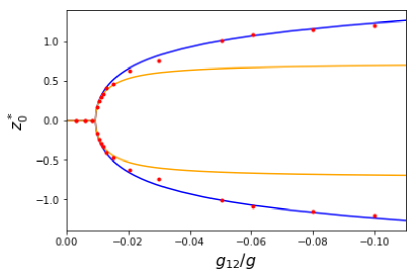
Figure 10: (Color online) Fixed points of the effective double well potential given by Eq. (21) (continuous blue line) as a function of $g_{12}/g$. The continuous (orange) line represents the analytical result (24) and the (red) dots are the mean position of the soliton oscillations extracted from the numerical solution of GP equation.

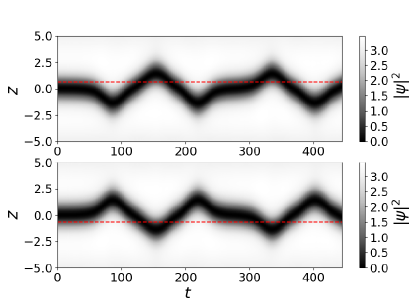
Figure 11: Spatio-temporal evolution of a dark-dark-soliton density obtained from the numerical solution of the GP Eq. (1) for $g_{12}/g=-0.046$ and harmonic trapping $\Omega=0.1$. Each panel corresponds to a different condensate. The dashed (red) lines represent the position of the equilibrium points given by (24).

We have numerically solved the GP Eq. (1) for the real-time evolution of  dark-dark solitons with values of $g_{12}$ below and above the bifurcation point $g_{c}$ for the change of stability. First, we have computed a case (see Fig. 11) with overlapped solitons situated at $z_{0}=0$ and $g_{12}/g=-0.046<g_{c}$, hence unstable according to the linear prediction. The initial stationary state has been perturbed with white-noise of $1\%$ amplitude. As expected the system is unstable, and eventually the solitons separate by moving towards the minima of the effective double well potential Eq. (24). In this case, each dark soliton has enough energy to pass through the energy barrier created at the trap center $z_{0}=0$, so that collisions between them are observed to cause a shift in their trajectories.

If instead the two dark solitons are initially situated at different locations, close to the positions of the fixed points Eq. (24) (see Fig. 12), the solitons oscillate symmetrically around such points. Their time evolution can be fitted by $x(t)=z_{0}^{*}+\left(-z_{0}^{*}+z_{0}\right)\cos(w_{\rm eff}t)$, where $w_{\rm eff}$ is given by (25), and provides a good approximation to the real time evolution obtained from the GP equation.

Figure 12: Same as Fig. 11 with $g_{12}/g=-0.0125$. In this spatio-temporal evolution each dark soliton is situated off center ($z_{0}=\pm 0.3$, near the equilibrium points given by (24)). The continuous line is fitted according to our analytical results (see text).

III.2.2 Repulsive interaction between condensates: ${g_{12}>0}$

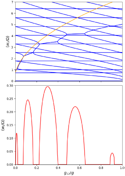
Figure 13: (Color online) Numerical results from the Bogoliubov spectrum of a dark-dark soliton with $\mu=10\,\Omega$ in a trap. The real (top panel) and imaginary (bottom panel) parts of the excitation frequencies are shown against the interaction strength ratio $g_{12}/g$. The continuous (orange) line represents the analytical values from Eq. (15).

Figure 13 represents the excitation spectrum of overlapped dark-dark solitons at $z_{0}^{*}=0$, in the range $g_{12}/g\in[0,1]$, for $\mu=10\,\Omega$, within the Thomas Fermi regime of the axial harmonic oscillator. At $g_{12}=0$, corresponding to uncoupled solitons, the linear modes have double degeneracy, and the lowest energy excitations are the anomalous mode, with frequency $\omega_{0}=\Omega/\sqrt{2}$, and the hydro-dynamical excitations $\omega_{n}=\sqrt{{n(n+1)}/{2}}\,\Omega$, with $n=1,2,...$ Stringari1996 ; Busch2000 ; Kevrekidis2015 ; Frantzeskakis2010 . The degeneracy is broken for non null $g_{12}$ and gives rise to two branches of in-phase and out-of-phase modes. In the hydro-dynamical case, the in-phase modes are associated to excitations in the total density of the background, and remain constant for varying $g_{12}$. On the other hand, the out-of-phase or spin modes account for variations in the difference of the background densities Abad2013 , and decrease their energy for increasing values of $g_{12}$.

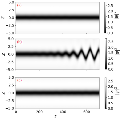
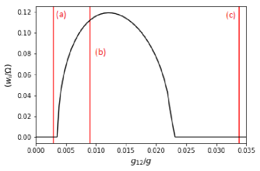
Figure 14: Real time evolution of three dark-dark solitons with varying coupling out of and inside the first instability region of Fig. 13, showing corresponding stable and unstable dynamics.

The anomalous modes are characterized by the negative value of the quantity $norm\times energy$ MacKay1987 , and in scalar condensates their frequency coincide with the oscillation frequency of the solitons in the trap Busch2000 . There are also two different anomalous modes for non null $g_{12}$, an in-phase one with constant energy, and an out-of-phase mode whose energy increases with $g_{12}$. The in-phase anomalous mode is associated with the small amplitude, abreast oscillations of the solitons in the trap, hence it is the same as in decoupled condensates: $\omega_{0}=\Omega/\sqrt{2}$. However, the out-of-phase anomalous mode is associated with the relative motion of the solitons. This mode, given by the analytical expression Eq. (23), is depicted (orange line) in the upper panel of Fig. 13, in good agreement with the numerical results for small values of $g_{12}/g$.

The lower panel of Fig. 13 present our numerical results for the imaginary part of the spectrum. As previously commented in the untrapped case, these instabilities are characterized by the collision of the out-of-phase anomalous mode with the spin mode associated with the background. These collisions produce Hamiltonian-Hopf bifurcations where a complex frequency quartet appears in the excitation spectrum. It is interesting to see that the out-of-phase anomalous mode only collides with odd spin modes. Regions of stability and instability alternates up to a value of the coupling with $g_{12}/g$ close to 1, but interestingly inside the immiscible regime. The higher the chemical potential, the closer is this value to $g_{12}/g=1$, according with the Bogoliubov analysis for the untrapped case. Such a value can be well approximated within the Thomas-Fermi regime by Eq. (40) evaluated at maximum density $n=\mu/(g+g_{12})$. Again the crossing of this analytical frequency with the function for small oscillations Eq. (23) provides a good estimate for the beginning of the first instability region in the range $g_{12}/g\in[0,1]$. It is worth noticing that such instability is not captured by Eq. (23) alone, due to the fact that for its derivation the soliton motion was assumed to be decoupled from the background.

Figure 14 shows examples of stable and unstable dark-dark solitons near the first instability region of Fig. 13. The evolution of the nonlinear systems develops according the linear stability analysis and demonstrate the existence of dynamically stable coupled solitons, cases (a) and (c), that could be experimentally realized.

IV Conclusions

The dynamics of dark-dark soliton states in two density coupled BECs has been studied within GP theory. By performing a perturbation analysis in the parameter $g_{12}/g$ for solitons with equal chemical potential, we have derived analytical expressions describing their relative motion both in harmonic traps and untrapped systems. Contrary to the case of solitons in scalar condensates, our theoretical model predicts that the interaction between dark solitons excited in different condensates is attractive (repulsive) for repulsive (attractive) interparticle interactions $g_{12}$. In harmonically trapped systems, the scenario is specially interesting for negative $g_{12}$, where the effective potential felt by the solitons modifies its shape as a function of $g_{12}$ (through a pitchfork bifurcation) from a single-well potential to a double-well potential, then allowing for stationary states made of solitons located at different positions.

The theoretical analytical predictions have been shown to be in good agreement with the numerical solutions of the Gross Pitaevskii equation for the real time evolution, and with the Bogoliubov equations for the linear excitations of the dark-dark solitons. In particular, we have demonstrated that the resonance of two out-of-phase modes, the anomalous one giving the frequency of the relative motion between solitons, and the lowest energy mode associated to the spin density excitation of the background, give rise to instabilities (Hopf bifurcations) that produce the decay of dark-dark solitons. This fact translate in finite systems, either harmonically trapped condensates or ring geometries, into alternating regions of dynamical stability and instability.

The existence of dynamically stable dark-dark solitons open up the way for their experimental realization. The current availability of Feshbach resonances for tuning both interaction parameters $g$ and $g_{12}$ allows to choose a stable fringe in the spectrum. Also in this regard, as a natural extension of this work, it would be interesting to explore the stability of equivalent states (soliton-soliton or vortex-vortex states) in multidimensional systems.

Appendix: Bogoliubov equations for overlapping dark solitons without external trap

In this case, the ground state of Eqs. (1) is the constant density solution $\psi_{1}(x)=\psi_{2}(x)=\sqrt{n}$, such that $\mu=(g+g_{12})n$. The dark soliton solutions healing to the ground state with density $n$ are given by

$$\psi_{1,2}(x)=\psi_{d}(x)e^{-i\mu\,t/\hbar}=\sqrt{\frac{\mu}{g+g_{12}}}\,\tanh\left(\frac{x}{\xi}\right)e^{-i\mu\,t/\hbar}\,,$$ (42)

where $\xi=\sqrt{\hbar^{2}/m\mu}$ is the soliton healing length. As in the scalar case, it can be seen that the soliton state depends on both, the chemical potential $\mu$ and the (sum of the) interaction strength $g+g_{12}$.

We check the stability of Eq. (42) by solving the Bogoliubov equations

$$H_{0}\,u_{1}+\psi_{d}^{2}\left[(2g+g_{12})u_{1}+gv_{1}+g_{12}(u_{2}+v_{2})\right]=\omega\,u_{1}$$

$$-H_{0}\,v_{1}-\psi_{d}^{2}\left[(2g+g_{12})v_{1}+gu_{1}+g_{12}(u_{2}+v_{2})\right]=\omega\,v_{1}$$

$$H_{0}\,u_{2}+\psi_{d}^{2}\left[(2g+g_{12})u_{2}+gv_{2}+g_{12}(u_{1}+v_{1})\right]=\omega\,u_{2}$$

$$-H_{0}\,v_{2}-\psi_{d}^{2}\left[(2g+g_{12})v_{2}+gu_{2}+g_{12}(u_{1}+v_{1})\right]=\omega\,v_{2},$$ (43)

where $H_{0}=-(\hbar^{2}/2m)\partial_{xx}-\mu$, and $[u_{1}(x),v_{1}(x),u_{2}(x),v_{2}(x)]$ are the linear modes with energy $\omega$.

By adding and substracting the the two first previous equations, on the one hand, and the two last, on the other hand, we obtain new equations for the linear combinations $f_{j\pm}=u_{j}(x)\pm v_{j}(x)$

$$\left(\frac{-\hbar^{2}}{2m}\partial_{xx}+\,(g+g_{12})\,\psi_{d}^{2}-\mu\right)f_{1-}=\omega f_{1+}$$

$$\left(\frac{-\hbar^{2}}{2m}\partial_{xx}+\,(g+g_{12})\,\psi_{d}^{2}-\mu\right)f_{2-}=\omega f_{2+},$$ (44)

$$\left(\frac{-\hbar^{2}}{2m}\partial_{xx}+(3g+g_{12})\psi_{d}^{2}\,-\mu\right)f_{1+}+2g_{12}\psi_{d}^{2}f_{2+}=\omega f_{1-}\,$$

$$\left(\frac{-\hbar^{2}}{2m}\partial_{xx}+(3g+g_{12})\psi_{d}^{2}\,-\mu\right)f_{2+}+2g_{12}\psi_{d}^{2}f_{1+}=\omega f_{2-}\,.$$ (45)

The first two equations Eqs. (44) are already decoupled for the modes $1$ and $2$, and (for $\omega=0$) contains zero energy excitations associated to the $U(1)$ symmetry presented within each condensate, so that a global phase can be arbitrarily picked in the soliton solutions Eq. (42). However, Eqs. (45) are still coupling the modes $1$ and $2$. In order to decouple them, we make the symmetric $f_{s\pm}=f_{1\pm}(x)+f_{2\pm}(x)$ and antisymmetric $f_{a\pm}=f_{1\pm}(x)-f_{2\pm}(x)$ linear combinarions to get

$$\left(\frac{-\hbar^{2}}{2m}\partial_{xx}+\,(g+g_{12})\,\psi_{d}^{2}-\mu\right)f_{s-}=\omega f_{s+}$$

$$\left(\frac{-\hbar^{2}}{2m}\partial_{xx}+3(g+g_{12})\psi_{d}^{2}\,-\mu\right)f_{s+}=\omega f_{s-}\,,$$ (46)

and

$$\left(\frac{-\hbar^{2}}{2m}\partial_{xx}+\,(g+g_{12})\,\psi_{d}^{2}-\mu\right)f_{a-}=\omega f_{a+}\,$$

$$\left(\frac{-\hbar^{2}}{2m}\partial_{xx}+(3g-g_{12})\psi_{d}^{2}\,-\mu\right)f_{a+}=\omega f_{a-}\,.$$ (47)

Equations (46) for the symmetric combinations $f_{s\pm}=f_{1\pm}(x)+f_{2\pm}(x)$ are equivalent to the Bog equations of a scalar condensate in a dark soliton state for an interaction strength $g+g_{12}$. As a result they do not present unstable modes, and contain two Goldstone modes (with $\omega=0$) reflecting the mentioned $U(1)$ symmetry and the translational invariance of the system.

On the other hand, the Eqs. (47) for the antisymmetric combinations $f_{a\pm}=f_{1\pm}(x)-f_{2\pm}(x)$ are relevant for the unstable modes having complex frequencies $\omega$. These modes can first appear at $\omega=0$ for particular values of the system parameters $\{\mu,g,g_{12}\}$ (for a given particle species of mass $m$), indicating a bifurcation of the soliton solutions giving place to a new stationary state. However, as we have seen in the text, the instabilities can also appear from a couple of nonzero real frequencies which become complex, indicating a Hopf bifurcation with a subsequent oscillatory dynamics. Below, we analyze the first case associated to the existence of zero modes.

At $\omega=0$, since the first equation (46) provides the commented Goldstone modes, we only have to look for solutions to

$$\left(\frac{-\hbar^{2}}{2m}\partial_{xx}+\mu\frac{3g-g_{12}}{g+g_{12}}\,\tanh^{2}\left(\frac{x}{\xi}\,\right)-\mu\right)f_{a+}=0\,,$$ (48)

that in units of the healing length gives

$$-\frac{1}{2}\partial_{xx}f_{a+}-(1+\delta g)\,\mbox{sech}^{2}(x)f_{a+}=-\delta g\,f_{a+},$$ (49)

where $\delta g=2(g-g_{12})/({g+g_{12}})=2(g-g_{12})n/\mu$ is the relevant parameter for the emergence of instabilities. Eq. (49) is a Schrödinger equation for the asymmetric wavefunction $f_{a+}$ in the potential well $\mbox{sech}^{2}(x)$ with depth $(1+\delta g)$. This well has bound states with energy $-\delta g$ whenever Rosen ; Sophie2017

$$\sqrt{2\,\delta g+\frac{9}{4}}-\sqrt{2\,\delta g}-\frac{1}{2}=n\,,$$ (50)

with $n=0,1,2,\dots$ and $n\leq\sqrt{2\delta g+9/4}-1/2$. The latter condition ensures that $g_{12}<g$ and saturates with $g=g_{12}$ at the starting point of the inmiscible regime.