Spinful Aubry-André model in a magnetic field: Delocalization facilitated by a weak spin-orbit coupling

Abstract

We have incorporated spin-orbit coupling into the Aubry-André model of tight-binding electron motion in the presence of periodic potential with a period incommensurate with lattice constant. This model is known to exhibit an insulator-metal transition upon increasing the hopping amplitude. Without external magnetic field, spin-orbit coupling leads to a simple renormalization of the hopping amplitude. However, when the degeneracy of the on-site energies is lifted by an external magnetic field, the interplay of Zeeman splitting and spin-orbit coupling has a strong effect on the localization length. We studied this interplay numerically by calculating the energy dependence of the Lyapunov exponent in the insulating regime. Numerical results can be unambiguously interpreted in the language of the phase-space trajectories. As a first step, we have explained the plateau in the energy dependence of the localization length in the original Aubry-André model. Our main finding is that a very weak spin-orbit coupling leads to delocalization of states with energies smaller than the Zeeman shift. The origin of the effect is the spin-orbit-induced opening of new transport channels. We have also found that restructuring of the phase-space trajectories, which takes place at certain energies in the insulating regime, causes a singularity in the energy dependence of the localization length.

I Introduction

A standard description of electron motion in a one-dimensional quasiperiodic potential is based on the Aubry-André (AA) modelOriginal with tight-binding Hamiltonian

$$\hat{H}_{0}=-t\sum\limits_{n}\left(c_{n}^{\dagger}c_{n+1}+c_{n+1}^{\dagger}c_{n}\right)+V\sum\limits_{n}\cos(2\pi\beta n)c_{n}^{\dagger}c_{n},$$ (1)

where $c_{n}^{\dagger}$ is the creation operator of electron on $n$-th site, $t$ is the hopping integral, $V$ is the amplitude of modulation of the on-site energies, and $\beta^{-1}$ is the modulation period. Non-triviality of the AA model originates from the fact that, for irrational $\beta$, it exhibits a delocalization transition and yet contains no randomness.

The key finding of Ref. Original, is that the Hamiltonian Eq. (1) possesses self-duality: upon transformation from coordinate to the momentum space it retains its form after the interchange $V\leftrightarrow 2t$. The consequence of this dualitySokoloffReview is that, for $V>2t$, all eigenstates are exponentially localized with localization length scaling as $(V-2t)^{-1}$. From the perspective of physics, the importance of the AA model is that it captures the peculiarities of motion of a two-dimensional electron in a perpendicular magnetic field and a periodic potential.Hofstadter ; Azbel1979 ; Thouless1982

Early studies of the AA model Sokoloff1980 ; Suslov ; Soukoulis ; Thouless1983 ; Kohmoto ; Kohmoto1 were focused on the properties of localized eigenfunctions near the transition. Lately, the interest to the AA model has been revived DasSarmaEdges ; InOpticalLattice ; Flach2013 ; KaiSun+DasSarma2013 ; Shlyapnikov ; Interacting2015 ; InOpticalLattice1 ; QuenchDynamics ; AnomalousDiffusion ; SO+bosons ; NigelCooper ; ac-driven ; Skipetrov ; QuenchDynamics1 ; AAAdiabaticPumping . Nowadays, it is invoked to study different observable quantities in the presence of the quasiperiodic background. These studies were largely motivated by two groups of experiments Refs. Experiment2008, ; Experiment2015, ; Experiment2017, and Refs. Experiment2009, ; Experiment2012, ; Experiment2013, . In the experiment Ref. Experiment2008, the expansion of cold atoms loaded into an optical lattice was studied. One-dimensional modulation was formed as a result of interference of two laser beams. Localization transition, which takes place upon increasing the modulation amplitude, was demonstrated through the analysis of spatial and momentum distribution of atoms released from the lattice. In Refs. Experiment2015, , Experiment2017, the degree of localization of cold fermions in quasiperiodic optical lattice was monitored via the time evolution of the imbalance of population of different sites following a quench of system parameters.

In experiments of the second groupExperiment2009 ; Experiment2012 ; Experiment2013 , propagation of light along the axes of coupled waveguides has been studied. The centers of waveguides formed a periodic array, while their parameters were periodically modulated. Localization transition has been detected via the spreading of initially narrow wave packet across the lattice.

Cavity quantum electrodynamics with cold atomsOptomechanics0 ; Optomechanics1 offers an alternative approach to emulating the AA HamiltonianNigelCooper ; InOpticalLattice . Experimental advances motivated new theoretical studies towards the extension of the AA model. These studies include incorporation of interaction effectsShlyapnikov ; Interacting2015 , effects of the ac-driveac-driven , and the dynamics of a quenchQuenchDynamics ; QuenchDynamics1 .

Another recent development in the field of cold atoms is the possibility to impose Zeeman shifts and spin-orbit couplingSpielman ; Galitski-Spielman by illumination the condensate with lasers. This raises a question about the extension of the AA model to incorporate spin-dependent effects. We address this question in the present paper.

The result of incorporation of the Zeeman splitting, $2\Delta$, into the AA model is, obviously, two decoupled AA models for $\uparrow$ and $\downarrow$ spin projections. At the transition, $V=2t$, two delocalized states emerge at energies $\pm\Delta$. We will show that incorporation of spin-orbit coupling alone does not violate the duality and amounts to modification of the hopping matrix element, while the eigenstates for opposite chiralities remain degenerate.

Generalization of the AA model becomes nontrivial when both, Zeeman splitting and spin-orbit coupling, are incorporated. In this case, the duality is lifted. We studied the interplay of the two spin-dependent effects numerically. The results are interpreted in the limit of large modulation period, $\beta\ll 1$, when the semiclassical description and, thus, the language of phase-space trajectoriesPhaseSpaceTrajectories applies. Nontriviality of interplay of Zeeman splitting and spin-orbit coupling originates from peculiar structure of the phase-space trajectories and the evolution of this structure with energy. In the language of phase-space trajectories, delocalization transition corresponds to the connectivity of these trajectories both in coordinate and in momentum space.

Our main finding is that, in the vicinity of the delocalization transition, a weak spin-orbit coupling leads to metallization in the energy domain $(-\Delta,\Delta)$. The origin of the effect is that spin-orbit coupling opens new transport channels. These channels facilitate the coupling between disconnected trajectories, thus allowing to avoid tunneling. In general, we demonstrate that restructuring of the phase-space at certain energy causes an anomaly in the localization length at this energy even if the restructuring takes place in the insulating regime.

II phase-space trajectories and localization length in Aubry-André model in the semiclassical limit

II.1 AA model with long modulation period

The most transparent scenario of delocalization transition in the Aubry-André model was proposed in Ref. Suslov, . This scenario is based on simplification which becomes possible when the inverse period is small, $\beta\ll 1$, the fractional part, $\beta_{1}$, of $\beta^{-1}$ is small, and all the successive $\beta_{i}$, the fractional parts of $\beta_{i-1}^{-1}$, are small. In this limit the system is characterized by the hierarchy of periods

$$l_{1}\sim\frac{1}{\beta},~{}l_{2}\sim\frac{1}{\beta\beta_{1}},~{}...~{},~{}l_{n}\sim\frac{1}{\beta\beta_{1}\beta_{2}...\beta_{n-1}},~{}...$$ (2)

With $l_{n}$ growing exponentially with $n$, the renormalization-group procedure is applicable. As a first step, smallness of $\beta$ guarantees that a given period of the potential, $V(x)=V\cos(2\pi\beta x)$, contains many, $\sim\frac{1}{\beta}\left(\frac{V}{t}\right)$, levels. These levels are the eigenfunctions of the operator, $2t\cos{\hat{p}}+V(x)$, where the coordinate, $x=n$, and the momentum, ${\hat{p}}=-id/dx$, are treated as continuous variables.

By virtue of the same condition, $\beta\ll 1$, the levels are discrete, i.e. the overlap, $t^{(1)}$, of the wave functions in the neighboring periods is smaller than the level spacing. If a group of $\beta^{-1}$ sites is viewed as a “supersite”, which is the essence of the renormalization group transformation, then this overlap plays the role of a first-order hopping integral. On the other hand, with overlap neglected, the levels in the neighboring periods are mismatched. This mismatch, being the result of irrationality of $\beta$, plays the role of the first-order modulation amplitude, $V^{(1)}$, of the supersite energiesSuslov . As a result, original model Eq. (1) with parameters $t$, $V$, and the period, $\beta^{-1}$, transforms into the same model with renormalized parameters $t^{(1)}$, $V^{(1)}$, and the period, $\beta_{1}^{-1}$. From the fact that renormalized Hamiltonian possesses duality, the recurrent relation put forward in Ref. Suslov, has the form

$$\left(\frac{V^{(n+1)}}{2t^{(n+1)}}-1\right)\sim\frac{1}{\beta_{n}}\left(\frac{V^{(n)}}{2t^{(n)}}-1\right)\sim l_{n+1}\left(\frac{V}{2t}-1\right)^{n}.$$ (3)

The fact that the critical exponent in the AA model is equal to $1$ follows immediately from Eq. (3).

On the physical level, the above procedure captures how the allowed band at the step, $n$, breaks into $\frac{1}{\beta_{n+1}}$ allowed bands at the step $(n+1)$ (devil’s staircaseAzbel1979 ). On the quantitative level, besides the critical exponent, this description does not answer the basic question about the energy dependence of the localization length in the insulating regime. We focus on this question in our numerical study.

In numerics, the full-developed staircase cannot be captured. Still, with two spin-dependent effects incorporated, the duality of the model gets violated, so that the modification of the localization length turns out to be highly nontrivial.

II.2 Test of the numerical approach

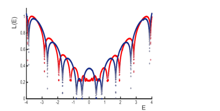
Figure 1: (Color online) Energy dependence of the Lyapunov exponent, $L(E)$, calculated numerically in the insulating regime with $t=0.4V$ for two values of $\beta$: commensurate $\beta=\frac{1}{10}$ (blue) and incommensurate $\beta=\frac{\sqrt{5}-1}{14}$ (red). While the values of $\beta$ are close to each other, $L(E)$ for incommensurate potential exhibits a plateau. The band-structure-induced wiggles are weak within the plateau. In the semiclassical limit, the plateau is expected in the interval $|E|<(V-2t)=0.2V$. Energy is measured in the units of $V/2$.

Numerical studies of the localization properties of eigenfunctions in AA model are carried out either by analysis of the inverse participation ratio, see e. g. Ref. DasSarmaEdges, , or by the analysis of eigenvalues of the transfer matrix, as in Ref. SO+bosons, . We have adopted the approach suggested in Ref. NUMERICAL, , which is based on the Thouless formula.Thouless1972 The object of interest is the behavior of the Lyapunov exponent, $L(E)$, which is the inverse localization length of the state with energy, $E$. The details of the computational procedure are presented in Appendix I. The analysis of the numerical data is complicated by the fact that irrational period of the potential, $\beta$, is approximated as a rational number in the computational process. For rational $\beta$, the exponent, $L(E)$, turns to zero within the energy bands, separated by the gaps. This causes “wiggles” in $L(E)$ obtained numerically. We call these wiggles, the band-structure effect. The problems caused by the band-structure effect become less acute as the value of $\beta$ is decreased. This is because the bands of allowed energies become progressively small. Still, it is important to note that, even at small $\beta$, the exponent, $L(E)$, calculated numerically, is distinctively different for incommensurate $\beta$. This is illustrated in Fig. 1, where the results for $L(E)$ are shown for two close values of $\beta$, one rational, $\beta=\frac{1}{10}$, and one irrational, $\beta=\frac{\sqrt{5}-1}{14}$. For irrational $\beta$, the expansion into continuous fraction has the form: $\beta_{1}=11$, $\beta_{2}=3$, $\beta_{3}=15$, and $\beta_{i}=\beta_{i-2}$ for $i>3$. The main difference between the two $L(E)$ curves is that, for irrational $\beta$, the $L(E)$-dependence exhibits a continuous plateau in the insulating regime, $V>2t$. The width of the plateau is $2(V-2t)$, reflecting the proximity to the transition. On the contrary, for rational $\beta$, $L(E)$ has two zeros in the plateau region connected by a smooth curve. This indicates that, for rational $\beta$, the behavior of eigenfunctions is not sensitive to the transition. Outside of the interval $|E|<(V-2t)$ both $L(E)$ curves have similar behavior. The difference between rational and irrational $\beta$ manifests itself in the fact that, for irrational $\beta$, the Lyapunov exponents, while exhibiting minima indicative of underdeveloped band-structure, never turns to zero.

III AA model in the semiclassical limit

As discussed in the previous Section, incommensurability manifests itself as a plateau in $L(E)$ dependence. Upon decreasing $\beta$, the plateau becomes progressively more pronounced. This is because wiggles in $L(E)$ get suppressed. This is illustrated in Fig. 2 for $\beta=\frac{\sqrt{5}-1}{29}$, i.e. two times smaller than in Fig. 1. It is important that, despite the presence of wiggles, the evolution of $L(E)$ across the metal-insulator transition can be clearly traced. The plateau in the insulating regime evolves into $L(E)\propto|E|$ at the transition. This is followed by a plateau $L(E)=0$ in the metallic regime. The behavior $L(E)\propto|E|$ in the interval $|E|<(V-2t)$ is in accord with general theorySuslov .

In this Section we demonstrate that, aside from wiggles, the behavior of $L(E)$ in Fig. 2 can be captured quantitatively within the semiclassical description. For small $\beta$ the potential changes slowly, which allows to introduce a local dispersion law at a given $x$. This law has a form

$$E(p,x)=V\cos(2\pi\beta x)+2t\cos p.$$ (4)

The equation Eq. (4) defines a system of phase-space trajectories,PhaseSpaceTrajectories $E(p,x)=E$. These trajectories are illustrated in Fig. 3.

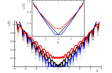
Figure 2: (Color online) Manifestation of the delocalization transition in the energy dependence of the Lyapunov exponent. The curves, $L(E)$, calculated numerically for $\beta=\frac{\sqrt{5}-1}{29}$ and for the same hopping integrals as in Fig. 3: $t=0.4V$ (red), $t=0.5V$ (black), and $t=0.66V$ (blue), are shown. Wiggles in the curves reflect the “band-structure effect,” as in Fig. 1. Still, the smooth parts of the curves clearly indicate the transition from insulator to metal. These smooth parts are described very well by $L(E)$ calculated analytically from Eqs. (5) and (6) and shown in the inset.

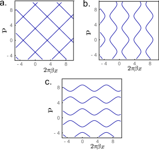
Figure 3: (Color online) Phase-space trajectories in the AA model are shown for zero energy and for three values of the hopping integral: $t=0.5V$ (a), $t=0.4V$ (b), and $t=0.66V$ (c). Trajectories in (b) “percolate” in the $p$-direction, while the trajectories in (c) percolate in the $x$-direction.

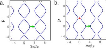
Figure 4: (Color online) Illustration of the origin of a plateau in $L(E)$ which develops in the interval $|E|<(V-2t)$ in the insulating regime. (a) For energies outside of this interval the coupling of the phase-space trajectories separated by a period involves a one-step tunneling at $p=0$, which is the shortest tunneling path. (b) For energies inside the interval this coupling involves a two-step tunneling at $p=0$ (green arrow) and $p=\pi$ (red arrow). As follows from Eq. 7, the logarithm of the tunneling amplitude for the first step is proportional to $(V-2t+E)$, while for the second step this logarithm is proportional to $(V-2t-E)$. Thus, the product of the amplitudes does not depend on $E$.

In the semiclassical limit, the duality, $p\leftrightarrow 2\pi x$ and $V\leftrightarrow 2t$, becomes apparent. In the language of phase-space trajectories, the metallic and the insulating states correspond to the trajectories continuous in the $x$-direction and discontinuous in $x$-direction, respectively. Metal-insulator transition at $V=2t$ takes place when the trajectories, corresponding to $E=0$, “percolate”. The energy dependence of the Lyapunov exponent at the transition point is determined by tunnel coupling of the trajectories disconnected in the $x$-direction. It follows from Eq. (4) that the tunneling takes place either along the line ${\text{Re}}~{}p=0$ or along the line ${\text{Re}}~{}p=\pi$. These points correspond to the minimal separation of the disconnected trajectories, see Fig. 4. Using Eq. (4), the semiclassical expression for the logarithm of the coupling constant, $\int dx~{}{\text{Im}}\hskip 2.84526ptp$, calculated along ${\text{Re}}~{}p=0$, can be cast in the form

$${\cal L}_{1}=\frac{1}{\pi\beta}\int\limits_{0}^{\cosh^{-1}\left(\frac{V+E}{2t}\right)}dq\frac{q\sinh q}{\sqrt{\big{(}\frac{V+E}{2t}-\cosh q\big{)}\big{(}\frac{V-E}{2t}+\cosh q\big{)}}}.$$ (5)

Corresponding expression for tunneling along ${\text{Re}}~{}p=\pi$ reads

$${\cal L}_{2}=\frac{1}{\pi\beta}\int\limits_{0}^{\cosh^{-1}\left(\frac{V-E}{2t}\right)}dq\frac{q\sinh q}{\sqrt{\big{(}\frac{V+E}{2t}+\cosh q\big{)}\big{(}\frac{V-E}{2t}-\cosh q\big{)}}}.$$ (6)

The upper limit in Eq. (5) corresponds to the first bracket in the denominator turning to zero, while the upper limit of Eq. (6) corresponds to the second bracket in the denominator turning to zero. If the argument in $\cosh^{-1}$ is smaller than $1$, the corresponding ${\cal L}$ should be set to zero.

At critical value $V=2t$ only ${\cal L}_{1}$ is nonzero for $E>0$, while only ${\cal L}_{2}$ is nonzero for $E<0$. For $E\ll t$ we can expand $\cosh q$ in the first bracket and replace $\cosh q$ by $1$ in the second bracket. Then the integral can be readily evaluated yielding

$${\cal L}_{1}=\frac{1}{\beta}\left(\frac{E}{4t}\right).$$ (7)

To relate ${\cal L}_{1}$ to the Lyapunov exponent, we reason as follows. Tunnel coupling of two trajectories separated in the $x$-direction by $n$ periods is $\exp(-n{\cal L}_{1})$. The distance between this trajectories is $x_{n}=\frac{n}{\beta}$. Expressed via the Lyapunov exponent, this coupling is $\exp(-Lx_{n})$. Thus, $L$ and ${\cal L}_{1}$ are related as $L=\beta{\cal L}_{1}$. We then conclude that the semiclassical result Eq. (7) captures the behavior of the Lyapunov exponent at the transition obtained numerically and shown in Fig. 2.

Consider now the vicinity of the transition $0<(V-2t)\ll t$. In the domain $|E|>(V-2t)$ only one of ${\cal L}_{1}$, ${\cal L}_{2}$ is nonzero, as it was at the transition. Then the generalization of Eq. (7), valid for arbitrary sign of $E$, takes the form

$$L(E)=\frac{|E|+(V-2t)}{4t}.$$ (8)

In the domain $|E|<(V-2t)$ both ${\cal L}_{1}$ and ${\cal L}_{2}$ are nonzero. The Lyapunov exponent is determined by the sum

$$L(E)=\beta\left({\cal L}_{1}+{\cal L}_{2}\right).$$ (9)

It is easy to see that the energy drops out from this sum, so that

$$L(E)=\frac{(V-2t)}{2t}$$ (10)

in this domain. The results Eq. (8) and Eq. (10) are plotted in Fig. 2, inset. We see that they completely agree with numerical results shown in the same figure. The expression for $L(0)$ is in accord with critical exponent of the AA model being equal to $1$.Suslov

We note that the simulation of the $L(E)$-dependence was previously carried out in Ref. NUMERICAL, . To suppress the band-structure effects the on-site energies were chosen in the form $V\cos(2\pi\beta|n|^{\nu})$, with $\nu=0.7$, so that the results did not depend on whether or not $\beta$ is irrational. Numerical results in Ref. NUMERICAL, are quite similar to those shown in Fig. 2, inset. However, the authors did not have an explanation for the plateau.

It is instructive to illustrate the $L(E)$-behavior in the AA model with the help of Fig. 4. Coupling between two phase-space trajectories separated by a period, $1/\beta$, requires tunneling. For $|E|>(V-2t)$, the geometry of the trajectories is such that this tunneling is a one-step process, see Fig. 4a. By contrast, for $|E|<(V-2t)$ the geometry of the trajectories is different, so that one-step tunneling is insufficient for the transport along $x$. Rather, the coupling is a product of the amplitudes of tunneling at $p=0$ and $p=\pi$. Upon the change of energy, one amplitude grows, while the other amplitude drops off, so that their product remains constant. Note finally, that the linear behavior of $L(E)$ given by Eq. (8) also applies for $V<2t$, outside the metallic domain, $|E|<(2t-V)$.

IV Delocalization in the presence of the Zeeman splitting: effect of a weak spin-orbit coupling

Zeeman splitting is incorporated into the AA model by adding the term $\Delta\sigma$ to the on-site energies, where $\sigma$ takes the values $\pm 1$. Presence of spin-orbit coupling allows a spin-flip process upon hopping to the neighboring sitejapanese . For hopping, say, to the right, we denote the corresponding hopping amplitude with $it_{1}$. Then, for hopping to the left, this amplitude is $-it_{1}$. With Zeeman splitting and spin-orbit coupling included, the Hamiltonian Eq. (1) takes the form

$$\hat{H}=-t\sum\limits_{n,\sigma}\left(c_{n,\sigma}^{\dagger}c_{n+1,\sigma}+c_{n+1,\sigma}^{\dagger}c_{n,\sigma}\right)\\ -it_{1}\sum\limits_{n,\sigma\neq\sigma^{{}^{\prime}}}\left(c_{n,\sigma}^{\dagger}c_{n+1,\sigma^{{}^{\prime}}}-c_{n+1,\sigma^{{}^{\prime}}}^{\dagger}c_{n,\sigma}\right)\\ +\sum\limits_{n,\sigma}\Big{[}V\cos(2\pi\beta n)+\Delta\sigma\Big{]}c_{n,\sigma}^{\dagger}c_{n,\sigma}.$$ (11)

In the semiclassical limit, the Hamiltonian Eq. (11) defines two branches of the spectrum and, correspondingly, two types of the phase-space trajectories. They are described by the equations

$$V\cos(2\pi\beta x)+2t\cos p\pm\Big{[}\Delta^{2}+4t_{1}^{2}\sin^{2}p\Big{]}^{1/2}=E.$$ (12)

It is easy to see that, without Zeeman splitting, the effect of spin-orbit coupling amounts to the replacement of $t$ by $\pm\left(t^{2}+t_{1}^{2}\right)^{1/2}$. This observation is, actually, general, i.e. it is valid not only in the semiclassical limit. As demonstrated in Appendix II, it can be derived rigorously from the Hamiltonian Eq. (11). Transformation $t\rightarrow\pm\left(t^{2}+t_{1}^{2}\right)^{1/2}$ is accompanied by the shift of momentum. Equally, it is obvious that without spin-orbit coupling, the eigenstates of the Hamiltonian Eq. (11) are the same as in Eq. (1) with eigenvalues shifted by $\pm\Delta$.

Our prime finding is that the interplay of the two spin-dependent processes has a dramatic effect on the localization properties of the eigenstates. More specifically, very small spin-orbit coupling leads to a strong suppression of the localization. This is illustrated in Fig. 5. The dependence, $L(E)$, in this figure was calculated for parameters $V$ and $t$ corresponding to the criticality, so that for, $t_{1}=0$, we obtained two $V$-shaped curves centered at $E=\pm\Delta$. After a small $t_{1}=0.05V$ was included, the behavior of $L(E)$ near $\pm\Delta$ did not change. However, $L(E)$ dropped down significantly in a wide domain of intermediate energies $|E|<V$.

The physics underlying this stark suppression of localization is the following. Small $t_{1}$ opens new channels of coupling between the trajectories corresponding to a given spin. Obviously, for $t_{1}=0$, all eigenstates corresponding to the branches Eq. (12) are orthogonal to each other. With finite $t_{1}$, the eigenstates corresponding to a given momentum are orthogonal to each other. However, the eigenstates corresponding to different momenta have a finite overlap. Below we confirm this statement by a direct calculation.

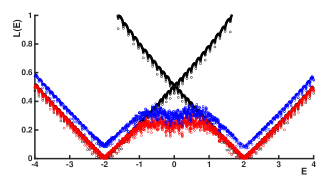
Figure 5: (Color online) Illustration of the effect of spin-orbit coupling on the localization in the AA model with Zeeman splitting. All the curves show $L(E)$ calculated for the critical value $t=0.5V$. Zeeman splitting is chosen to be $\Delta=V$. Black lines are $L(E)$ calculated for $t_{1}=0$. They correspond to the metal-insulator transitions at energies $E=\pm\Delta$. Incorporation of a weak spin-orbit coupling, $t_{1}=0.05V$, suppresses the localization in the domain $-\Delta<E<\Delta$. Blue and red numerical curves are for two eigenvalues of the transmission matrix (see the text). For clarity, the calculation was performed for large period, $\beta=\frac{\sqrt{5}-1}{97}$.

The analytical forms of the eigenfunctions corresponding to $+$ and $-$ branches are the following:

$$\Psi_{p}^{+}=\begin{pmatrix}\varphi_{1p}^{+}\\ \\ \varphi_{2p}^{+}\end{pmatrix}=\frac{1}{2^{1/2}D_{p}^{1/4}(D_{p}-\Delta)^{1/2}}\begin{pmatrix}-2it_{1}\sin p\\ \\ \Delta-D_{p}\end{pmatrix},$$ (13)

$$\Psi_{p}^{-}=\quad\begin{pmatrix}\varphi_{1p}^{-}\\ \\ \varphi_{2p}^{-}\end{pmatrix}=\frac{1}{2^{1/2}D_{p}^{1/4}(D_{p}+\Delta)^{1/2}}\begin{pmatrix}-2it_{1}\sin p\\ \\ \Delta+D_{p}\end{pmatrix},$$ (14)

where $D_{p}$ is defined as

$$D_{p}=\left(\Delta^{2}+4t_{1}^{2}\sin^{2}p\right)^{1/2}.$$ (15)

Using Eqs. (13) and (14), we calculate the scalar product of $+$ and $-$ eigenfunctions with different momenta and obtain

$$\langle\Psi_{p+\frac{q}{2}}^{-}|\Psi_{p-\frac{q}{2}}^{+}\rangle=-\frac{4t_{1}^{2}\Delta\sin\frac{q}{2}\cos p}{(D_{p+\frac{q}{2}}D_{p-\frac{q}{2}})^{1/4}[(D_{p+\frac{q}{2}}+\Delta)(D_{p-\frac{q}{2}}-\Delta)]^{1/2}}\\ \times\Bigg{[}\frac{\Delta\sin\frac{q}{2}\cos p}{\Delta^{2}+4t_{1}^{2}\sin(p+\frac{q}{2})\sin(p-\frac{q}{2})+D_{p+\frac{q}{2}}D_{p-\frac{q}{2}}}+2\frac{\cos\frac{q}{2}\sin p}{D_{p+\frac{q}{2}}+D_{p-\frac{q}{2}}}\Bigg{]}.$$ (16)

It is easy to see that this product is zero when either $\Delta=0$, $t_{1}=0$, or the transferred momentum, $q$, is equal to zero.

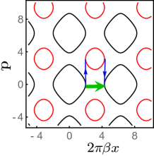
Figure 6: (Color online) Schematic illustration of the spin-orbit facilitated delocalization. The phase-space trajectories for a given energy $E<\Delta$ include the contours corresponding to two different branches, see Eq. (12). They are shown with black and red lines. Coupling between two black contours is determined either by tunneling (green arrow) or by two virtual transitions from black to red and back (blue arrows). These transitions are accompanied by change of the momentum by $\pi$, so that the corresponding spinors are not orthogonal, see Eq. (16). Moreover, the amplitudes of these transitions are proportional to $t_{1}$ but do not contain tunneling exponent. Thus, already at very small $t_{1}$, these transitions dominate the coupling. As a result, $L(E)$ drops dramatically, as shown in Fig. 5. The contours in the figure are shown for parameters: $\Delta=V$, $t=0.5V$ (as in Fig. 5), and for $E=0.5V$.

Now we can explain the behavior of $L(E)$ in Fig. 5. The phase-space trajectories corresponding to intermediate energies are shown in Fig. 6. Black contours correspond to $+$ branch, while red contours correspond to $-$ branch. Direct coupling between two black contours requires tunneling shown with green arrow. Note, however, that the coupling can be realized by a two-step process via an intermediate red contour: first the virtual transition from black to red, shown by a left blue arrow, and then the transition from red to shifted black contour, shown by a right blue arrow. It can be easily shown that the momentum transfer in both virtual transitions is $\pi$, so that the blue lines are vertical.

For small $t_{1}$, the amplitude of the two-step process is small $\propto t_{1}^{2}$. On the other hand, it does not contain the tunneling exponent. Thus, this process dominates the Lyapunov exponent when $L(E)$ calculated for direct tunneling is bigger than $|\ln t_{1}^{2}|$. We have checked this prediction numerically. The results are shown in Fig. 7. It can be seen that the plateau in $L(E)$ at intermediate energies indeed scales with $|\ln t_{1}^{2}|$.

To conclude the Section, we demonstrated that for energies, at which the phase-space trajectories corresponding to both branches coexist, a particle can avoid tunneling by “bouncing” between the states of different branches. It should be emphasized that this effect is specific only for tight-binding model in which the bandwidth is limited.

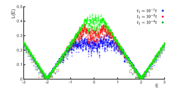
Figure 7: (Color online) Scaling of the plateau in $L(E)$ with spin-orbit strength, $t_{1}$. The plateau height calculated for three $t_{1}$-values drops, upon increasing $t_{1}$, as $|\ln\left(t_{1}/t\right)|$. Parameters $\Delta$, $t$ and the period, $\beta$, are the same as in Fig. 5.

V Delocalization due to spin-orbit coupling alone

In previous Section we assumed that the amplitude, $t_{1}$, of hopping with spin-flip constitutes a small correction to the spin-conserving hopping amplitude, $t$. In the present Section we show that interplay of Zeeman splitting and spin-orbit coupling alone, without direct hopping, can result in nontrivial effects in localization properties of the AA model.

Upon setting $t=0$ in Eq. (12), the equations for the phase-space trajectories assume the form

$$\pm\Big{[}\Delta^{2}+4t_{1}^{2}\sin^{2}p\Big{]}^{1/2}-E=V\cos(2\pi\beta x).$$ (17)

Although the duality between $x$ and $p$ is absent, both branches still exhibit the delocalization transition for certain relation between $t_{1}$, $\Delta$, and $V$. To find this relation and the energy position of the delocalized state, we reason as follows. Upon changing $p$ from $0$ to $\pi/2$, the combination in the left-hand side of Eq. (17) changes from $\left(\Delta-E\right)$ to $\left[\left(\Delta^{2}+4t_{1}^{2}\right)^{1/2}-E\right]$, while the combination in the right-hand side changes from $-V$ to $V$ upon changing $x$. To achieve percolation of phase-space trajectories, one should require that these intervals of change coincide. This leads to the conditions

$$\Delta-E=-V,$$ (18)

$$\left(\Delta^{2}+4t_{1}^{2}\right)^{1/2}-E=V.$$ (19)

Upon solving the above system, we find the critical value of $t_{1}$ and percolation energy, $E^{c}$,

$$\frac{t_{1}^{c}}{V}=\Bigg{[}\frac{|\Delta|}{V}+1\Bigg{]}^{1/2},~{}~{}~{}\pm\frac{E^{c}}{V}=\frac{|\Delta|}{V}+1.$$ (20)

The Lyapunov exponent, $L(E)$, calculated for critical value, $t_{1}=t_{1}^{c}$, and for one value of $t_{1}$ below the transition are shown in Fig. 8a. We see that quantum delocalization indeed takes place at critical $t_{1}$. As illustrated in Fig. 8b, the phase-space trajectories at $t_{1}=t_{1}^{c}$ and $E=E^{c}$ are not perfect squares. This is the reflection of the absence of $x$-$p$ duality. This duality is respected only near the crossing points, like $(x,p)=(0,\pi/2)$, but it is these points that are responsible for transport.

Energies $\pm E^{c}$ correspond to delocalization within individual branches. Most nontrivial scenario emerges when both branches are involved in transport. We will demonstrate that, for a certain relation between $t_{1}$, $V$, and $\Delta$ there is an anomaly in the behavior of the localization length with energy inside the insulator regime. This relation is established from the condition that the energy distance between the branches is equal to $2V$ and has the form

$$\frac{4\left({\tilde{t}}_{1}^{c}\right)^{2}}{V^{2}}+\frac{\Delta^{2}}{V^{2}}=1.$$ (21)

Firstly, at this $t_{1}$, the phase-space trajectories corresponding to both branches coexist. They are shown by blue and red lines in Fig. 9. The value $t_{1}={\tilde{t}}_{1}^{c}$ is distinguished by the fact that the restructuring of the phase-space trajectories corresponding to $E=0$ takes place at this $t_{1}$. Note that the restructuring at $t_{1}={\tilde{t}}_{1}^{c}$ does not involve percolation, as it is illustrated in Fig. 9.

The restructuring of the phase-space trajectories affects the transport for the following reason. As seen in Fig. 9b, for $t_{1}>{\tilde{t}}_{1}^{c}$, the transport is exclusively due to tunneling between blue and red trajectories. On the contrary, for $t_{1}<{\tilde{t}}_{1}^{c}$ the transport requires both: inter-branch tunneling between blue and red trajectories as well as intra-branch tunneling between blue trajectories and between red trajectories. This is because for $t_{1}<{\tilde{t}}_{1}^{c}$ additional classically forbidden regions appear, see Fig. 9c.

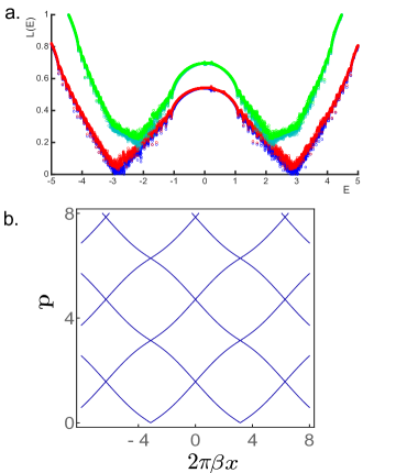
Figure 8: (Color online) Illustration of delocalization transition at zero direct hopping $(t=0)$. The transfer between the sites is exclusively due to finite spin-orbit coupling. (a): the dependencies $L(E)$, calculated for $\Delta=2V$ and for two values of $t_{1}$ are shown: (red) $t_{1}=1.72V$ and (green) $t_{1}=1.22V$. For the first value, the condition Eq. (20) is satisfied, so that the phase-space trajectories for $E=E_{c}=3V$, shown in (b), percolate. For the second value, $L(E)$ exhibits the plateau-like behavior near the minimum. The underlying reason for this is that the transport between disconnected phase-space trajectories involves two types of tunneling similar to Fig. 4b. Energy in the figure is measured in the units of $V$.

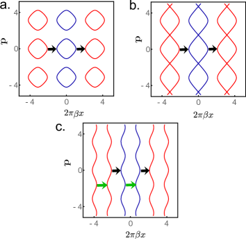
Figure 9: (Color online) Phase-space trajectories at zero energy and in the absence of direct hopping are shown for parameters $t_{1}=0.433V$ (a), $t_{1}=0.333V$ (b), $t_{1}=0.485V$ (c). Zeeman splitting is chosen to be $\Delta=0.5V$ in all three plots.

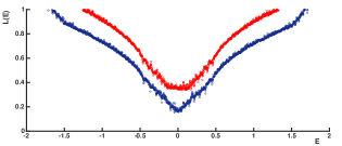
Figure 10: (Color online) The dependencies, $L(E)$, are shown for $t=0$, $\Delta=0.5V$ and two values of $t_{1}$: (blue) $t_{1}={\tilde{t}}_{1}^{c}=0.433V$ and (red) $t_{1}=0.35V$. The blue curve exhibits a $V$-shaped behavior which reflects the restructuring of the phase-space trajectories. The red curve exhibits a plateau around $E=0$. This plateau has the similar origin as the plateau in Fig. 2. Energy is measured in the units of $V$.

Restructuring of the trajectories at $t_{1}={\tilde{t}}_{1}^{c}$ leads to the anomaly in the energy dependence of the Lyapunov exponent. Namely, $L(E)$ exhibits a $V$-shape behavior, as shown in Fig. 10. The origin of this behavior is the following. The minimal value, $L(0)$, is determined by the inter-branch tunneling. For positive $E$, transport requires additional tunneling between the red trajectories. For negative $E$, transport requires additional tunneling between the blue trajectories. This additional tunneling takes place at $p=\pi/2$. The “price” of additional tunneling is proportional to $E$, as we have established above, see Eq. (7). Thus, the behavior of $L(E)$ at small $E$ has the form

$$\left(L(E)-L(0)\right)\propto|E|.$$ (22)

Note that the tunneling between red and blue trajectories is “forbidden”, in the sense, that the initial and final states are both at $p=0$. Thus, the corresponding spinors are orthogonal to each other. The reason why this tunneling still takes place is the uncertainty in the momentum, $\delta p$, of a tunneling particle. This uncertainty can be viewed as a momentum transfer in the course of tunneling. Then the overlap integral Eq. (16) can be estimated as $\delta p/\Delta$. The uncertainty is set by the discreteness of the AA model, i.e. by the fact that the coordinate in Eq. (17) takes integer values. This yields, $\delta p\sim\beta^{-1}$.

For $t_{1}$ slightly smaller than ${\tilde{t}}_{1}^{c}$, a plateau in $L(E)$ develops in the vicinity of $E=0$. The origin of this plateau is absolutely similar to the origin of the plateau around zero energy for $t_{1}=0$ and finite $t$ slightly smaller than $0.5V$.

VI Conclusion

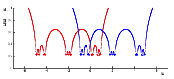
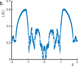
Figure 11: (Color online) The Lyapunov exponent as a function of energy is plotted for canonical $\beta=\frac{\sqrt{5}-1}{2}$ in the insulating regime, $t=0.4V$. Zeeman splitting is chosen to be $\Delta=V$. In the upper panel, (a), spin-orbit coupling is absent. In the lower panel, (b), the parameter $t_{1}$ is chosen to be $t_{1}=0.05V$. It is seen that two plots differ only near $E=0$, where small $t_{1}$ causes the metallization. Blue and red curves in (b) correspond to two eigenvalues of the transmission matrix. Energy is measured in the units of $V/2$.

To illustrate our findings, we presented the numerical results for large modulation periods, $\beta\ll 1$. For these periods the semiclassical description applies, which allowed us to interpret the findings in the language of the phase-space trajectories. In most studies, however, the inverse “golden mean” value, $\beta=\frac{\sqrt{5}-1}{2}$, is employed. For this period, the localization properties of the eigenstates in the insulating regime are most complex, in the sense, that $L(E)$ takes very different values for close energies. This “band-structure-induced” wiggles in $L(E)$ are most pronounced in the vicinity of the transition, as is illustrated in Fig. 2 (black curve). We emphasize that the effect of delocalization due to small $t_{1}$ persists for canonical $\beta=\frac{\sqrt{5}-1}{2}$. In Fig. 11 we show the curves $L(E)$ for this value of $\beta$ calculated without spin-orbit coupling, $t_{1}=0$, and with weak spin-orbit coupling, $t_{1}=0.05V$, We see that finite $t_{1}$ makes almost no difference except for the domain near $E=0$, where it turns the insulator with $L(0)\approx 0.2$ into a metal.

It is instructive to put our main finding into a more general perspective. The closest analogy to the effect we report can be found in Ref. PRL1995, . In this paper the orbital motion of a 2D electron in a strong perpendicular magnetic field was considered. It was demonstrated that spin-orbit coupling between the Zeeman-split Landau levels assists the passage of electron through the saddle points of a smooth random potential, and, thus, facilitates delocalization.

Delocalizing effect of spin-orbit coupling in the quantum Hall regime is expectedKhmelnitskii to manifest itself via the splitting of the extended states in two overlapping spin subbands. This is in accord with later numerical simulationsLeeChalker ; HannaQuantumHall+SO

Concerning the standard physical mechanism of spin-orbit facilitating of delocalizationHikami , it is based on the suppression of constructive interference of two scattering paths related by time reversal. In two dimensions it leads to the crossover from weak localization to weak antilocalization in the magnetoresistance curves. It is inefficient in the problem we studied due to the presence of strong Zeeman splitting. Note finally, that quantization of the phase-space trajectories in a weak magnetic field in metals with strong spin-orbit couplingBeenakker ; Glazman had recently became a hot topic in relation to Weyl semimetals.

Acknowledgements

The work was supported by the Department of Energy, Office of Basic Energy Sciences, Grant No. DE- FG02-06ER46313.

VII Appendix I

We adopt and extend the numerical procedure, described in Ref. NUMERICAL, , to calculate the Lyapunov exponent, $L(E)$, for the Hamiltonian Eq. (11). Rewriting the Hamiltonian Eq. (11) in the form similar to that in Ref. NUMERICAL, one has

$$\hat{H}=\sum\limits_{n}\left(V_{n}I+\Delta\sigma_{z}\right)|\phi_{n}\rangle\langle\phi_{n}|\\ +T\sum\limits_{n}\Big{(}|\phi_{n}\rangle\langle\phi_{n+1}|+|\phi_{n+1}\rangle\langle\phi_{n}|\Big{)},$$ (23)

where $|\phi_{n}\rangle$ is a $2\times 1$ vector

$$\phi_{n}=\begin{pmatrix}\psi_{n}^{\uparrow}\\ \\ \psi_{n}^{\downarrow}\end{pmatrix},$$ (24)

and $\psi_{n}^{\uparrow(\downarrow)}$ corresponds to up(down) spin projections. The matrices $I$ and $\sigma_{z}$ are the identity matrix and the Pauli matrix, respectively. The $2\times 2$ matrix, $T$, has the meaning of the transmission matrix and has the form

$$T=\begin{pmatrix}t&&it_{1}\\ \\ -it_{1}&&t\end{pmatrix}.$$ (25)

The diagonal terms, $V_{n}=V\cos\left(2\pi\beta n\right)$, stand for on-site energies. Parameters $\Delta$, $t$, $t_{1}$ are defined in the main text.

The numerical procedure in Ref. NUMERICAL, is based on step-by-step decimation of sites achieved by renormalization of energies and coupling matrix elements for remaining sites. Since $V_{n}$ is an even function of $n$, we can restrict consideration to $n\geq 0$.

As a first step, consider three sites $n=0$, $n=1$, and $n=2$. Elimination of the site $n=1$, results in the following renormalization of the bare on-site energies, $\left(V_{n}I-\Delta\sigma_{z}\right)$, of the sites $n=0$, and $n=2$, as well as renormalization of coupling, $T_{\scriptscriptstyle 0,2}$,

$$\varepsilon_{\scriptscriptstyle 0}^{\scriptscriptstyle 1}(E)=\left(V_{0}I-\Delta\sigma_{z}\right)+T^{\dagger}\left(E-V_{1}I+\Delta\sigma_{z}\right)^{-1}T,$$

$$\varepsilon_{\scriptscriptstyle 2}^{\scriptscriptstyle 1}(E)=\left(V_{2}I-\Delta\sigma_{z}\right)+T^{\dagger}\left(E-V_{1}I+\Delta\sigma_{z}\right)^{-1}T,$$

$$T_{\scriptscriptstyle 2,0}(E)=T^{\dagger}\left(E-V_{1}I+\Delta\sigma_{z}\right)^{-1}T.$$ (26)

Renormalized energies, $\varepsilon_{0}^{1}(E)$, and $\varepsilon_{2}^{1}(E)$ serve as bare energies in the subsequent elimination steps. At the second step, the site $n=2$ is eliminated using the rules prescribed by Eq. (VII). Repeating this procedure $N-1$ times, one arrives to the system of two sites, $n=0$ and $n=N$, with effective on-site energies and effective coupling in the form

$$\varepsilon_{\scriptscriptstyle 0}^{\scriptscriptstyle N-1}(E)=\varepsilon_{\scriptscriptstyle 0}^{\scriptscriptstyle N-2}(E)+T_{\scriptscriptstyle 0,N-1}\Big{[}E-\varepsilon_{\scriptscriptstyle N-1}^{\scriptscriptstyle N-2}(E)\Big{]}^{-1}T_{\scriptscriptstyle N-1,0}(E).$$ (27)

$$\varepsilon_{\scriptscriptstyle N}^{\scriptscriptstyle N-1}(E)=\varepsilon_{\scriptscriptstyle N}^{\scriptscriptstyle N-2}(E)+T_{\scriptscriptstyle 0,N-1}(E)\Big{[}E-\varepsilon_{\scriptscriptstyle N-1}^{\scriptscriptstyle N-2}(E)\Big{]}^{-1}T_{\scriptscriptstyle N-1,0}(E).$$ (28)

$$T_{\scriptscriptstyle N,0}(E)=T_{\scriptscriptstyle 0,N}^{\dagger}(E)=T_{\scriptscriptstyle 0,N-1}\Big{[}E-\varepsilon_{\scriptscriptstyle N-1}^{\scriptscriptstyle N-2}(E)\Big{]}^{-1}T.$$ (29)

In Ref. NUMERICAL, the Lyapunov exponent is defined as

$$L(E)=-\lim\limits_{\scriptscriptstyle N\rightarrow\infty}\frac{1}{N}\ln|\lambda_{\scriptscriptstyle N}(E)|,$$ (30)

where $\lambda_{\scriptscriptstyle N}(E)$ is the eigenvalue of the effective coupling matrix, $T_{\scriptscriptstyle 0,N}$. In the presence of the Zeeman splitting and the spin-orbit coupling the eigenvalues are non-degenerate, which results in two Lyapunov exponents. Only the smallest of these two values should be identified with the inverse localization length.

VIII Appendix II

In the presence of both direct hopping, $t$, and spin-orbit coupling, $t_{1}$, one can write the tight binding equations for AA model as

$$V\cos(2\pi\beta n)f_{n}+t(f_{n+1}+f_{n-1})+t_{1}(g_{n+1}-g_{n-1})\\ \hskip 156.49014pt=Ef_{n},\\ V\cos(2\pi\beta n)g_{n}+t(g_{n+1}+g_{n-1})-t_{1}(f_{n+1}-f_{n-1})\\ =Eg_{n},$$ (31)

where $f_{n},g_{n}$ are the amplitudes at site $n$, corresponding to the up spin and to the down spin. Fourier transformations of $f_{n}$ and $g_{n}$ can be written as follows:

$$f_{n} = \sum\limits_{m}A_{m}\exp[2im\pi\beta n]\exp(ikn),$$

$$g_{n} = \sum\limits_{m}B_{m}\exp[2im\pi\beta n]\exp(ikn)$$ (32)

Substituting Eq. (VIII) in Eq. (31) and then comparing the coefficients of $\exp[2im\pi\beta n]\exp(ikn)$ we arrive at

$$\frac{V}{2}\Big{[}A_{m+1}+A_{m-1}\Big{]}+2t\cos(2\pi\beta m+k)A_{m}\\ \hskip 48.36967pt+2it_{1}\sin(2\pi\beta m+k)B_{m}=EA_{m},\\ \frac{V}{2}\Big{[}B_{m+1}+B_{m-1}\Big{]}+2t\cos(2\pi\beta m+k)B_{m}\\ -2it_{1}\sin(2\pi\beta m+k)A_{m}=EB_{m}.$$ (33)

Multiplying the first equation by $i$ and then adding/subtracting it to/from the second equation yields

$$\frac{V}{2}\Big{[}A_{m+1}\pm iB_{m+1}+A_{m-1}\pm iB_{m-1}\Big{]}\\ +2\ \sqrt{t^{2}+t_{1}^{2}}\cos(2\pi\beta m+k\mp k_{0})\Big{[}A_{m}\pm iB_{m}\Big{]}=E\Big{[}A_{m}\pm iB_{m}\Big{]},$$ (34)

where

$$k_{0}=\arctan\frac{t_{1}}{t},$$ (35)

and $A\pm iB$ are the new amplitudes. We have reduced the AA model with spin-orbit coupling to two decoupled AA models for a spinless electron with hopping amplitude $\left(t^{2}+t_{1}^{2}\right)^{1/2}$. It is important that, while the eigenvalues of Eqs. (34) are the same for $+$ and $-$ signs, the corresponding eigenvectors are not orthogonal to each other.

References

- (1) S. Aubry and G. André, “Analyticity Breaking and Ander- son Localization in Incommensurate Lattices,” Ann. Isr. Phys. Soc. 3, 133 (1980).
- (2) J. B. Sokoloff, “Unusual band structure, wave functions and electrical conductance in crystals with incommensurate periodic potentials,” Phys. Rep. 126, 189 (1985).
- (3) D. R. Hofstadter, “Energy levels and wave functions of Bloch electrons in rational and irrational magnetic fields,” Phys. Rev. B 14, 2239 (1976).
- (4) M. Ya. Azbel, “Quantum Particle in One-Dimensional Potentials with Incommensurate Periods,” Phys. Rev. Lett. 43 1954 (1979).
- (5) D. J. Thouless, M. Kohmoto, M. P. Nightingale, and M. den Nijs, “Quantized Hall Conductance in a Two-Dimensional Periodic Potential,” Phys. Rev. Lett. 49, 405 (1982).
- (6) J. B. Sokoloff, “Electron localization in crystals with quasiperiodic lattice potentials,” Phys. Rev. B 22, 5823 (1980).
- (7) I. M. Suslov, “Localization in one-dimensional incommensurate systems,” Zh. Eksp. Teor. Fiz. 83 1079 (1982) [Sov. Phys. JETP 56 612 (1982)].
- (8) C. M. Soukoulis and E. N. Economou, “Localization in One-Dimensional Lattices in the Presence of Incommensurate Potentials,” Phys. Rev. Lett. 48, 1043 (1982).
- (9) D. J. Thouless, “Bandwidths for a quasiperiodic tight-binding model,” Phys. Rev. B 28, 4272 (1983).
- (10) M. P. Kohmoto, L. P. Kadanoff, and C. Tang,“Localization Problem in One Dimension: Mapping and Escape,” Phys. Rev. Lett. 50, 1870 (1983).
- (11) M. P. Kohmoto, “Metal-Insulator Transition and Scaling for Incommensurate Systems,” Phys. Rev. Lett. 51, 1198 (1983).
- (12) J. Biddle and S. Das Sarma, “Predicted Mobility Edges in One-Dimensional Incommensurate Optical Lattices: An Exactly Solvable Model of Anderson Localization,” Phys. Rev. Lett. 104, 070601 (2010).
- (13) L. Zhou, H. Pu, K. Zhang, X.-D. Zhao, and W. Zhang, “Cavity-induced switching between localized and extended states in a noninteracting Bose-Einstein condensate,” Phys. Rev. A 84, 043606 (2011).
- (14) K. Rayanov, G. Radons, and S. Flach, “Decohering localized waves,” Phys. Rev. E 88, 012901 (2013).
- (15) V. P. Michal, B. L. Altshuler, and G. V. Shlyapnikov, “Delocalization of Weakly Interacting Bosons in a 1D Quasiperiodic Potential,” Phys. Rev. Lett. 113, 045304 (2014).
- (16) V. Mastropietro, “Localization of Interacting Fermions in the Aubry-André Model,” Phys. Rev. Lett. 115, 180401 (2015).
- (17) K. Rojan, R. Kraus, T. Fogarty, H. Habibian, A. Minguzzi, and G. Morigi, “Localization transition in the presence of cavity backaction,” Phys. Rev. A 94, 013839 (2016).
- (18) C. Yang, Y. Wang, P. Wang, X. Gao, and S. Chen, “Dynamical signature of localization-delocalization transition in a one-dimensional incommensurate lattice,” Phys. Rev. B 95, 184201 (2017).
- (19) E. Gholami and Z. M. Lashkami, “Noise, delocalization, and quantum diffusion in one-dimensional tight-binding models,” Phys. Rev. E 95, 022216 (2017).
- (20) S. Ray, B. Mukherjee, S. Sinha, and K. Sengupta, “Bosons with incommensurate potential and spin-orbit coupling,” Phys. Rev. A 96, 023607 (2017).
- (21) W. Zheng and N. R. Cooper, “Anomalous Diffusion in a Dynamical Optical Lattice,” arXiv:1709.03916.
- (22) S. Ray, A. Ghosh, and S. Sinha, “Drive Induced Delocalization in Aubry-André Model,” arXiv:1709.04018.
- (23) A. Sinha and S. E. Skipetrov, “Time-dependent reflection at the localization transition,” arXiv:1709.06828.
- (24) Q.-B. Zeng, S. Chen, and R. Lü, “Quench dynamics in the Aubry-André-Harper model with p-wave superconductivity,” arXiv:1710.05256.
- (25) X. L. Zhao, Z. C. Shi, C. S. Yu, and X. X. Yi, “Influence of localization transition on dynamical properties for an extended Aubry-André-Harper model,” J. Phys. B 50, 235503 (2017).
- (26) S. Ganeshan, K. Sun, and S. Das Sarma, “Topological Zero-Energy Modes in Gapless Commensurate Aubry-André-Harper Models,” Phys. Rev. Lett. 110, 180403 (2013).
- (27) G. Roati, C. D’Errico, L. Fallani, M. Fattori, C. Fort, M. Zaccanti, G. Modugno, M. Modugno, and M. Inguscio, “Anderson localization of a non-interacting Bose-Einstein condensate,” Nat. Lett. 453, 895 (2008).
- (28) M. Schreiber, S. S. Hodgman, P. Bordia, H, P. Lüschen, M. H. Fischer, R. Vosk, E. Altman, U. Schneider, and I. Bloch, “Observation of many-body localization of interacting fermions in a quasirandom optical lattice,” Science 349, 842 (2015).
- (29) P. Bordia, H. Lüschen, U. Schneider, M. Knap, and I. Bloch, “Periodically driving a many-body localized quantum system,” Nat. Phys. 13, 460 (2017).
- (30) Y. Lahini, R. Pugatch, F. Pozzi, M. Sorel, R. Morandotti, N. Davidson, and Y. Silberberg, “Observation of a Localization Transition in Quasiperiodic Photonic Lattices,” Phys. Rev. Lett. 103, 013901 (2009).
- (31) Y. E. Kraus, Y. Lahini, Z. Ringel, M. Verbin, and O. Zilberberg, “Topological States and Adiabatic Pumping in Quasicrystals,” Phys. Rev. Lett. 109, 106402 (2012).
- (32) M. Verbin, O. Zilberberg, Y. E. Kraus, Y. Lahini, and Y. Silberberg, “Observation of topological phase transitions in photonic quasicrystals,” Phys. Rev. Lett. 110, 076403 (2013).
- (33) P. Maunz, T. Puppe, I. Schuster, N. Syassen, P. W. H. Pinkse, and G. Remp, “Cavity cooling of a single atom,” Nature 428, 50 (2004).
- (34) H. Ritsch, P. Domokos, F. Brennecke, and T. Esslinger, “Cold atoms in cavity-generated dynamical optical potentials,” Rev. Mod. Phys. 85, 553 (2013).
- (35) Y.-J. Lin1, R. L. Compton, K. Jiménez-Garcia, J. V. Porto, and I. B. Spielman, “Synthetic magnetic fields for ultracold neutral atoms,” Nature 462, 628 (2009).
- (36) V. Galitski and I. B. Spielman, “Spin-orbit coupling in quantum gases,” Nature 494, 49 (2013).
- (37) M. Albert and P. Leboeuf, “Localization by bichromatic potentials versus Anderson localization,” Phys. Rev. A 81, 013614 (2010).
- (38) R. Farchioni, G. Grosso, and G. P. Parravicini, “Electronic structure in incommensurate potentials obtained using a numerically accurate renormalization scheme,” Phys. Rev. B 45, 6383 (1992).
- (39) D. J. Thouless, “A relation between the density of states and range of localization for one dimensional random systems,” J. Phys. C 5, 77 (1972).
- (40) T. Mii, N. Shima, K. Kano, and K. Makoshi, “Spin-Orbit Interaction in the Tight-Binding Model: Toward the Comprehension of the Rashba Effect at Surfaces,” J. Phys. Soc. Jpn. 83, 064706 (2014).
- (41) D. G. Polyakov and M. E. Raikh, “Quantum Hall Effect in Spin-Degenerate Landau Levels: Spin-Orbit Enhancement of the Conductivity,” Phys. Rev. Lett. 75, 1368 (1995).
- (42) “Quantum Hall effect without Landau quantization,” Helv. Phys. Acta. 65, 164 (1992).
- (43) D. K. K. Lee and J. T. Chalker, “Unified model for two localization problems: Electron states in spin-degenerate Landau levels and in a random magnetic field,” Phys. Rev. Lett. 72, 1510 (1994).
- (44) C. B. Hanna, D. P. Arovas, K. Mullen, and S. M. Girvin, Phys. Rev. B 52, 5221 (1995).
- (45) S. Hikami, A. I. Larkin, and Y. Nagaoka, “Spin-orbit interaction and magnetoresistance in the two dimensional random system,” Prog. Theor. Phys. 63, 707 (1980).
- (46) T. E. O’Brien, M. Diez, and C. W. J. Beenakker, Phys. Rev. Lett. 116, 236401 (2016).
- (47) A. Alexandradinata and L. Glazman, “Modern theory of magnetic breakdown,” arXiv:1708.09387.