Abstract

Multiple quantum (MQ) NMR coherence spectra, which can be obtained experimentally in MQ NMR, can be transferred from the sender to the remote receiver without mixing the MQ-coherences of different orders and distortions. The only effect of such transfer is scaling of the certain blocks of sender’s density matrix (matrices of MQ-coherences of different order). Such a block-scaled transfer is an alternative to the perfect state transfer. In particular, equal scaling of higher order MQ-coherences matrices is possible. Moreover, there are states which can be transferred to the receiver preserving their zero-order coherence matrix. The examples of block-scaled transfer in spin-1/2 communication lines of 6 and 42 nodes with two-qubit sender and receiver are presented.

I Introduction

The problem of remote state creation is an intensively developing direction in quantum information processing. Having been formulated by Bose in Ref.Bose as a problem of pure state transfer, it has undergone many modifications since that time. First of all, we should mention the papers regarding perfect state transfer based on the fully engineered spin chain CDEL ; ACDE ; KS and high-probability state transfer based on chains with remote GKMT ; WLKGGB ; FKZ_2010 and optimized BACVV2010 ; ZO ; BACVV2011 ; ABCVV ; SAOZ end-bonds.

The next series of papers refers to manipulating the parameters of the remotely created states. Here, first of all, we shall cite the experiments with photons PBGWK2 ; PBGWK ; XLYG , where photon polarizations appear as creatable parameters. The interest in other two-level systems as material suitable for remote state creation appears in Ref.LH . Recently, different aspects of state creation in spin-1/2 chains have been considered: the optimization of creatable region via local unitary transformations of sender and extended receiver Z_2014 ; BZ_2015 ; BZ_2016 , the remote manipulation of multi-quantum coherences FKZ_2016 , the creation of particular two-qubit states SZ_2016 .

Evolution of quantum state unavoidably destroys the density matrix initially settled at the sender. There are three basic destroying processes: dispersion (due to the complicated spectrum of a propagating signal), decay (due to the interaction with environment) and element mixing. The latter is, in particular, the consequence of the dispersion and is absent, for instance, in the case of perfect state transfer CDEL ; ACDE ; KS . However, the perfect state transfer is a mathematical model which is hardly realizable in practice. Therefore, the development of a tool allowing to reconstruct the sender’s initial matrix from the matrix registered at the receiver is a problem of principal importance.

In our paper we concentrate on studying the states that can be transferred from the sender to the receiver with minor, well characterizable deformation avoiding mixing of matrix elements. In the ideal case, the only deformation would be scaling the matrix elements which can take arbitrary values satisfying the requirements of positivity and normalization for the density matrix. Such states can serve as carriers of quntum information encoded into the elements of a density matrix.

In this regard we refer to Ref.FZ_2017 , where the MQ-coherence matrices were shown to evolve independently under the Hamiltonian conserving the excitation number in a spin system. Hence we can study the transfer of a state of several interacting qubits from the sender to the receiver without mixing MQ NMR coherences of different orders during the transfer process. The interest in these matrices is intimately connected with the new possibilities given by multiple quantum (MQ) NMR in solids allowing to observe experimentally MQ NMR coherences of different orders. In turn, MQ NMR dynamics is a powerful tool for studying the nuclear spin distributions in various systems BMGP ; DMF including a nanopore DFZ_2011 . Therefore, there are numerous papers studying the coherence matrices as a whole object (for instance, in terms of coherence intensities). In particular, the dynamics and relaxation of MQ coherences in solids were considered in Ref.KS1 ; KS2 ; AS ; CCGR ; BFVV . It was shown in Ref.FZ_2017 that the MQ-coherence matrices do not mix during the evolution under the Hamiltonian conserving the number of excited spins. However, the matrix elements inside of each such matrix do mix during the evolution. We propose a way of overcoming this mixing.

Our basic results can be stated as follows.

1. Each MQ-coherence matrix of the properly selected sender’s initial state can evolve without mixing its elements. This process leads to the minimal deformation of the transferred state and can be an alternative to the perfect state transfer.

2. In certain cases the evolution of each MQ-coherence matrix reduces to just multiplication by a constant parameter thus scaling it (block-scaled states).

3. The sender’s zero-order coherence matrix of a special structure can be perfectly transferred to the receiver’s zero-order coherence matrix.

4. The scale factors can be the same for all the higher order coherence matrices.

5. All arguments in nn.2-4 are justified using examples of a two-qubit state transfer (i.e., we use the two-qubit sender and receiver) along the chains of 6 and 42 nodes. The creatable regions of the receiver state-space are characterized in all considered cases of the block-scaled transfer.

The paper has the following structure. General discussion of block-scaled states is given in Sec.II. Transfer of one-qubit block-scaled states is considered in Sec.III. The detailed study of two-qubit block-scaled state transfer is presented in Sec.IV. Basic results are discussed in Sec.V. Analytical derivation of the two-qubit state evolution and explicit formulas for the elements of the receiver density matrix are given in the Appendix, Sec.VI.

II Block-scaled states

The purpose of the initial state transfer from the sender to the receiver is obtaining the sender’s initial state at the receiver side at some time instant. However, the receiver state differs from the desired one in general. Usually, the evolution mixes all the elements of the initial state so that the elements of the receiver density matrix are linear combinations of all the elements of the sender’s initial density matrix. However, there might be special initial states and a special evolution Hamiltonian such that the elements of the receiver density matrix are proportional to the appropriate elements of the sender density matrix up to the normalization condition, i.e., for the $M$-qubit receiver,

$$\rho^{(R)}_{nm}=\lambda_{nm}\rho^{(S)}_{nm},\;\;(n,m)\neq(2^{M},2^{M}),$$ (1)

$$\rho^{(R)}_{2^{M}2^{M}}=1-\sum_{i=1}^{2^{M}-1}\rho^{(R)}_{ii},$$ (2)

where the parameters $\lambda_{nm}$ are called the scale factors (they do not depend on the initial state) and the $2^{M}\times 2^{M}$ density matrix $\rho^{(R)}$ is defined as

$$\rho^{(R)}=Tr_{/R}\rho(t),$$ (3)

where the trace is over the state space of the whole spin system except the receiver. Thus, the only non-scaled element of the density matrix $\rho^{(R)}$ is the diagonal element $\rho^{(R)}_{2^{M}2^{M}}$, because it is nesessary to satisfy the normalization condition, see Eq.(2). We notice that any diagonal element can be chosen for this purpose, although the obtained results depend on this choice, see Sec.III.

Relations (1,2) can be considered as a map of the elements of sender’s initial state density matrix to the elements of the receiver density matrix. This map performs the partial restoring of the sender’s initial state and can be realized, in particular, if the evolution is governed by the Hamiltonian conserving the number of excitations in the system, for instance, by the nearest neighbor $XX$-Hamiltonian,

$$H=\sum_{i=1}^{N-1}D(I_{ix}I_{(i+1)x}+I_{iy}I_{(i+1)y}),$$ (4)

where $D$ is a coupling constant. In this case, the MQ-coherence matrices evolve independently. We recall that the element of a density matrix $\rho^{(R)}$ contributes to the $\pm n$th coherence matrix $\rho^{(R;\pm n)}$ if it corresponds to the transition in the state space changing the excitation number by $\pm n$. Such evolution prompts us to present the density matrix $\rho^{(R)}$ as the sum

$$\rho^{(R)}=\sum_{i=1}^{M}\rho^{(R;i)},\;\;\rho^{(R;-i)}=(\rho^{(R;i)})^{+}.$$ (5)

Writing the sender’s and receiver’s zero-order coherence matrices as the sums

$$\rho^{(S;0)}=e^{(4)}+\tilde{\rho}^{(S;0)},\;\;\;\rho^{(R;0)}=e^{(4)}+\tilde{\rho}^{(R;0)},\;\;\;e^{(4)}={\mbox{diag}}(\underbrace{0,\dots,0}_{2^{M}-1},1),$$ (6)

we rewrite system (1,2) in the form

$$\rho^{(R;i)}_{nm}=\lambda^{(i)}_{nm}\rho^{(S;i)}_{nm},\;\;i=\pm 1,\dots,\pm M,\;\;\lambda^{(-i)}=(\lambda^{(i)})^{*}$$ (7)

$$\tilde{\rho}^{(R;0)}_{nm}=\lambda^{(0)}_{nm}\tilde{\rho}^{(S;0)}_{nm},$$

where $*$ means complex conjugate. In this way, we select $e^{(4)}$ as the non-scaled part (including just one non-zero element) of the receiver density matrix.

Next, we can require that scale factors for all elements from the each particular coherence matrix and from the matrix $\tilde{\rho}^{(S;0)}_{nm}$ in (7) are the same, $\lambda^{(i)}_{nm}\equiv\lambda^{(i)}$. Then (7) reduces to the following system:

$$\rho^{(R;i)}(t)=\lambda^{(i)}(t)\rho^{(S;i)}(0),\;\;i=\pm 1,\dots,\pm M,$$ (8)

$$\tilde{\rho}^{(R;0)}(t)=\lambda^{(0)}(t)\tilde{\rho}^{(S;0)}(0).$$

In other words, evolution scales the blocks of the sender’s initial state $\rho^{(S)}(0)$. We refer to receiver state (8) as the block-scaled state. System (8) can be considered as a map from the sender’s to the receiver’s coherence matrices. It is shown in Secs.III and IV that $|\lambda^{(i)}|<1$, $i>0$, so that the evolution compresses the higher-order coherence matrices, while $\lambda^{(0)}$ (which is real) can be either greater or smaller then unit.

Finally, we consider the case of equal scale factors for coherence matrices of all non-zero orders $|i|>0$ (uniform scaling): $\lambda^{(\pm M)}=\dots=\lambda^{(\pm 1)}=\lambda^{\pm}$, i.e.,

$$\rho^{(R;i)}=\lambda^{\pm}\rho^{(S;i)},\;\;i=\pm 1,\dots,\pm M,\;\;\;\lambda^{-}=(\lambda^{+})^{*},$$ (9)

$$\tilde{\rho}^{(R;0)}=\lambda^{(0)}\tilde{\rho}^{(S;0)}.$$

Hereafter, we study maps (8) and (9) with real scale factors:

$$\lambda^{(i)}=\lambda^{(-i)},\;\;\lambda^{-}=\lambda^{+}=\lambda.$$ (10)

III Communication line with one-qubit sender and receiver

Here, we consider the model of an $N$-node spin-communication line with one-node sender and receiver connected by the transmission line of $N-2$ spins. The problem of a pure state evolution in such a communication line was considered in Ref.FKZ_2016 ; here we remind the nesessary details.

The initial state in our model is a tensor product state

$$\rho(0)=\rho^{(S)}(0)\otimes\rho^{(TL,R)}(0),$$ (11)

where the sender state $\rho^{(S)}(0)$ is a pure one (we use the Dirac notations $|0\rangle$ and $|1\rangle$ for the ground and excited spin states, respectively):

$$\rho^{(S)}(0)=(a_{0}|0\rangle+a_{1}|1\rangle)(\langle 0|a_{0}^{*}+\langle 1|a_{1}^{*})=\left(\begin{array}[]{cc}1-|a_{1}|^{2}&a_{0}a_{1}^{*}\cr a_{0}^{*}a_{1}&|a_{1}|^{2}\end{array}\right),\;\;|a_{0}|^{2}+|a_{1}|^{2}=1,$$ (14)

and the state of the rest of the system is the thermal equilibrium one:

$$\rho^{(TL,R)}(0) = \frac{e^{bI_{z}}}{\left(2\cosh\frac{b}{2}\right)^{N-1}}.$$ (15)

Here $\displaystyle b=\frac{\hbar\omega_{0}}{kT}$ ($\hbar$ is the Planck constant, $\omega_{0}$ is the Larmor frequency of spins in the external magnetic field, $k$ is the Boltzmann constant, $T$ is the temperature), $I_{i}^{\pm}=I_{xi}\pm iI_{yi}$, $I_{\alpha i}$ is the $i$th spin projection on the $\alpha$-axis and $H$ is the $XX$ nearest neighbor Hamiltonian (4). The receiver density matrix reads FKZ_2016

$$\rho^{(R)}(t)=\left(\begin{array}[]{cc}\frac{e^{\frac{b}{2}}}{2\cosh\frac{b}{2}}+\frac{1}{2}\left(\frac{e^{-\frac{b}{2}}}{2\cosh\frac{b}{2}}-2|a_{1}|^{2}\right)|f(t)|^{2}&\left(-\tanh\frac{b}{2}\right)^{N-1}a_{0}a_{1}^{*}f^{*}(t)\cr\left(-\tanh\frac{b}{2}\right)^{N-1}a_{0}^{*}a_{1}f(t)&\frac{e^{-\frac{b}{2}}}{2\cosh\frac{b}{2}}-\frac{1}{2}\left(\frac{e^{-\frac{b}{2}}}{2\cosh\frac{b}{2}}-2|a_{1}|^{2}\right)|f(t)|^{2}\end{array}\right),$$ (18)

where

$$f(t)=\sum_{k=1}^{N}e^{i\varepsilon_{k}t}g_{1k}g_{Nk},\;\;\varepsilon_{k}=\cos\frac{\pi k}{N+1},\;\;g_{jk}=\left(\frac{2}{N+1}\right)^{1/2}\sin\frac{\pi jk}{N+1},\;\;j,k=1,\dots,N.$$ (19)

One can easily verify that $f$ is real for odd $N$ and imaginary for even $N$.

The partial restoring (7) with $M=1$ reads (the element $\rho^{(R)}_{22}$ provides normalization)

$$\rho^{(R;1)}_{12}=\lambda^{(1)}\rho^{(S;1)}_{12},$$ (20)

$$\rho^{(R;0)}_{11}=\lambda^{(0)}\rho^{(S;0)}_{11}.$$ (21)

Relation (20) always holds, and

$$\lambda^{(1)}=f^{*}\left(-\tanh\frac{b}{2}\right)^{N-1},$$ (22)

so that $\lambda^{(1)}$ is independent on the sender’s initial state. On the contrary, condition (21) yields

$$\lambda^{(0)}=\frac{-2e^{b}-|f|^{2}+2|a_{1}|^{2}|f|^{2}(1+e^{b})}{2(e^{b}+1)(|a_{1}|^{2}-1)}.$$ (23)

Therefore, $\lambda^{(0)}$ depends on the sender’s initial state in general (through the parameter $a_{1}$). However, if

$$|f|^{2}=\frac{2e^{b}}{1+2e^{b}},$$ (24)

then

$$\lambda^{(0)}=\frac{2e^{b}}{1+2e^{b}}\geq\frac{2}{3},\;\;b>0,$$ (25)

which is independent on the sender’s initial state. It can be shown numerically that condition (24) with $f$ given in (19) can be satisfied for $N\leq 17$. For the boundary value $N=17$ we have $|f|^{2}=0.6730$ at $t=19.6551$.

Another variant of the partial restoring reads (the element $\rho^{(R)}_{11}$ provides normalization)

$$\rho^{(R)}_{12}=\lambda^{(1)}\rho^{(S)}_{12},$$ (26)

$$\rho^{(R)}_{22}=\lambda^{(0)}\rho^{(S)}_{22}.$$ (27)

In this case, $\alpha_{22}$ depends on the initial state (the parameter $a_{1}$) as follows

$$\lambda^{(0)}=|f|^{2}+\frac{2-|f|^{2}}{2|a_{1}|^{2}(1+e^{b})}.$$ (28)

In the low temperature limit $b\to\infty$, Eq.(28) reduces to

$$\lambda^{(0)}=|f|^{2},$$ (29)

which is independent on the initial state. In this limit, we have

$$\rho^{(R)}(t)=\left(\begin{array}[]{cc}1-|a_{1}|^{2}|f(t)|^{2}&(-1)^{N-1}a_{0}a_{1}^{*}f^{*}(t)\cr(-1)^{N-1}a_{0}^{*}a_{1}f(t)&|a_{1}|^{2}|f(t)|^{2}\end{array}\right).$$ (32)

Thus, results of state restoring depend on our choice of the diagonal element providing normalization: the element $\rho^{(R)}_{22}$ in formulas (20)-(25) or the element $\rho^{(R)}_{11}$ in formulas (26)-(32).

III.1 Perfect transfer of zero-order coherence matrix

Unlike the higher-order coherence matrices, the zero-order coherence matrix can be perfectly transferred from the sender to the receiver along the homogeneous spin chain. In both cases, Eqs.(20),(21), (23) and Eqs.(26),(27), (28), the requirement

$$\lambda^{(0)}=1$$ (33)

yields

$$|a_{1}|^{2}=\frac{2-|f|^{2}}{2(1-|f|^{2})(1+e^{b})}.$$ (34)

This formula shows that the value of $|a_{1}|$ satisfying condition (33) decreases as $b$ increases and increases with $|f|$. In the limit $b\to\infty$, requirement (33) yields $|f|=1$ (perfect state transfer), so that condition (33) becomes independent on the parameter of the initial state $a_{1}$.

IV Communication line with two-qubit sender and receiver

Now, we consider the model of $N$-node spin-communication line with the two-node sender and two-node receiver connected by a transmission line of $N-4$ spins. The initial state of this system is a product state (11) where the sender state $\rho^{(S)}_{0}$ is an arbitrary mixed two-qubit state written as

$$\rho^{(S)}(0) = \frac{1}{4}E+a_{01}I_{z1}+a_{02}I_{z2}+a_{03}I_{z1}I_{z2}+a_{11}I_{2}^{-}+a_{11}^{*}I_{2}^{+}+a_{12}I_{z1}I_{2}^{-}+a_{12}^{*}I_{z1}I_{2}^{+}+$$

$$a_{13}I_{1}^{-}I_{2}^{+}+a_{13}^{*}I_{1}^{+}I_{2}^{-}+a_{21}I_{1}^{-}+a_{21}^{*}I_{1}^{+}+a_{22}I_{1}^{-}I_{z2}+a_{22}^{*}I_{1}^{+}I_{z2}+a_{31}I_{1}^{-}I_{2}^{-}+a_{31}^{*}I_{1}^{+}I_{2}^{+},$$

and the rest of the system is in the thermal equilibrium state,

$$\rho^{(TL,R)} = \frac{e^{bI_{z}}}{\left(2\cosh\frac{b}{2}\right)^{N-2}}.$$ (36)

Here, $H$ is the $XX$ nearest neighbor Hamiltonian (4). We notice that the nearest-neighbor Hamiltonian (4) and initial state (IV), (36) enable the analytical study of the spin dynamics. Using the Jordan-Wigner transformation JW ; CG we derive the evolution of the density matrix $\rho$ for a homogeneous spin-1/2 chain of arbitrary length $N$ and obtain the receiver state (3). The applied analytical approach allows us to avoid the numerical calculations in $2^{N}\times 2^{N}$ matrix space and study the state-propagation in long chains. The basic steps of constructing the density matrix for the receiver state are briefly outlined in Appendix.

The receiver density matrix (3) can be presented as the sum of the matrices $\rho^{(R;n)}$ contributing to the $n$th order coherence:

$$\rho^{(R)}=\sum_{n=-2}^{2}\rho^{(R;n)},$$ (37)

and the explicit formulas for the nonzero elements of the matrices $\rho^{(R;n)}$ are found analytically. Thus, for the zero order coherence we have

$$(\rho^{(R;0)})_{ij}=\alpha_{ij,11}\rho^{(S)}_{11}+\alpha_{ij,22}\rho^{(S)}_{22}+\alpha_{ij,33}\rho^{(S)}_{33}+\alpha_{ij,44}\rho^{(S)}_{44}+\alpha_{ij,23}\rho^{(S)}_{23}+\alpha_{ij,32}(\rho^{(S)}_{23})^{*},$$ (38)

$$(i,j)=(1,1),(2,2),(3,3),(4,4),(2,3),(3,2),$$

For the first order coherence:

$$(\rho^{(R;1)})_{ij}=\alpha_{ij,12}\rho^{(S)}_{12}+\alpha_{ij,13}\rho^{(S)}_{13}+\alpha_{ij;24}\rho^{(S)}_{24}+\alpha_{ij;34}\rho^{(S)}_{34},\;\;(i,j)=(1,2),(1,3),(2,4),(3,4),$$ (39)

Finally, for the second order coherence we have

$$\rho^{(R;2)}_{14}=\alpha_{14,14}\rho^{(S)}_{14}.$$ (40)

Thus, the elements of each matrix $\rho^{(R;n)}$ depend on the elements of the appropriate matrix $\rho^{(S;n)}$. The analytical expressions for the coefficients $\alpha_{ij;nm}$ in formulas (38) –(40) are given in Appendix, Eqs.(167)- (204).

IV.1 General properties of map (8), (10)

We consider block-scaling map (8), (10) with $M=2$ (we also write the inverse temperature $b$ as an argument) ,

$$\rho^{(R;\pm 2)}(t,b)=\lambda^{(2)}(t)\rho^{(S;\pm 2)}(0),$$ (41)

$$\rho^{(R;\pm 1)}(t,b)=\lambda^{(1)}(t,b)\rho^{(S;\pm 1)}(0),$$ (42)

$$\tilde{\rho}^{(R;0)}(t,b)=\lambda^{(0)}\tilde{\rho}^{(S;0)}(0),$$ (43)

and, first of all, treat Eqs.(41) – (43) as three independent maps without ensuring positivity for the density matrices consisting of the above coherence matrices.

The simplest map is Eq.(41). According to (40), the scale factor $\lambda^{(2)}$ in this map reads

$$\lambda^{(2)}(t)=\alpha_{14;14}(t).$$ (44)

This function is explicitly found in the Appendix, Eq.(204). It is an oscillating function with the first maximum at $t\sim N$, see Fig.1. Thus, this maxima for $N=6$ and $N=42$ read, respectively, $\lambda^{(2)}_{opt}=0.8960$ at $t_{opt}=8.5153$ and $\lambda^{(2)}_{opt}=0.2621$ at $t_{opt}=47.8855$.

Figure 1: Scale factor $\lambda^{(2)}$ as a function of $t$ for the spin chains of $N=6$ (thin line) and $N=42$ (bold line) nodes.

Next, map (42) concerning the $\pm 1$-order coherences is more complicated. It can be written as (for the 1-order coherence)

$$T^{(1)}(t,b)X^{(1)}=\lambda^{(1)}(t,b)X^{(1)},$$ (45)

where, in view of (39), $T^{(1)}$ and $X^{(1)}$ read:

$$T^{(1)}=\left(\begin{array}[]{cccc}\alpha_{12;12}&\alpha_{12;13}&\alpha_{12;24}&\alpha_{12;34}\cr\alpha_{13;12}&\alpha_{13;13}&\alpha_{13;24}&\alpha_{13;34}\cr\alpha_{24;12}&\alpha_{24;13}&\alpha_{24;24}&\alpha_{24;34}\cr\alpha_{34;12}&\alpha_{34;13}&\alpha_{34;24}&\alpha_{34;34}\cr\end{array}\right),\;\;X^{(1)}=\left(\begin{array}[]{c}\rho^{(S)}_{12}\cr\rho^{(S)}_{13}\cr\rho^{(S)}_{24}\cr\rho^{(S)}_{34}\end{array}\right).$$ (54)

In addition, $T^{(-1)}=(T^{(1)})^{*}$ and $X^{(-1)}=(X^{(1)})^{*}$. Eq.(54) is nothing but the eigenvalue problem for the matrix $T^{(1)}$, where the scale factor $\lambda^{(1)}$ is the eigenvalue and $X^{(1)}$ is the appropriate eigenvector. We can expect that both $\lambda^{(1)}$ and $X^{(1)}$ depend on $t$ and $b$ because $T^{(1)}$ does. The $4\times 4$ eigenvalue problem has four different eigenvalues in general, $\lambda^{(1)}_{i}$, $i=1,2,3,4$ (ordered by the absolute value $|\lambda_{1}|\geq|\lambda_{2}|\geq|\lambda_{3}|\geq|\lambda_{4}|$), associated with the eigenvectors $c^{(1)}_{i}X^{(1)}_{i}$ ($|X^{(1)}_{i}|=1$), where the arbitrary scalar factors $c^{(1)}_{i}$ are complex in general. Since we need only one eigenvector out of four (corresponding to the maximal by absolute value eigenvalue $\lambda_{1}$), we denote $c^{(1)}\equiv c^{(1)}_{1}$. As mentioned above, we consider only the real eigenvalues, which are presented over the plane $(b,t)$ in Fig.2 for $N=6$ in decreasing order from Fig.2a to Fig.2d. This figure shows that each eigenvalue $\lambda^{(1)}_{i}$ has a maximum as $b\to\infty$ at some instant $t$. The upper boundary lines in panels of Fig.2 separate the real eigenvalues (below these lines) from the complex ones (above the boundary lines) which are not shown in figure.

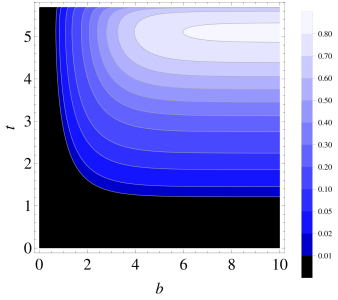
(a)

(b)

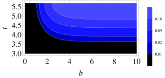
(c)

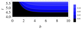
(d)

Figure 2: Four different eigenvalues $\lambda^{(1)}_{i}$ (see Eq.(45)) in decreasing order from (a) to (d) over the plane $(b,t)$ for the spin chain of $N=6$ nodes.

Finally, map (43) can be written as

$$T^{(0)}(t,b)X^{(0)}+B(t,b)=\lambda^{(0)}X^{(0)},$$ (55)

where

$$T^{(0)}=\left(\begin{array}[]{ccccc}\alpha_{11;11}-\alpha_{11;44}&\alpha_{11;22}-\alpha_{11;44}&\alpha_{11;33}-\alpha_{11;44}&\alpha_{11;23}&\alpha_{11;32}\cr\alpha_{22;11}-\alpha_{22;44}&\alpha_{22;22}-\alpha_{22;44}&\alpha_{22;33}-\alpha_{22;44}&\alpha_{22;23}&\alpha_{22;32}\cr\alpha_{33;11}-\alpha_{33;44}&\alpha_{33;22}-\alpha_{33;44}&\alpha_{33;33}-\alpha_{33;44}&\alpha_{33;23}&\alpha_{33;32}\cr\alpha_{23;11}-\alpha_{23;44}&\alpha_{23;22}-\alpha_{23;44}&\alpha_{23;33}-\alpha_{23;44}&\alpha_{23;23}&\alpha_{23;32}\cr\alpha_{32;11}-\alpha_{32;44}&\alpha_{32;22}-\alpha_{32;44}&\alpha_{32;33}-\alpha_{32;44}&\alpha_{32;23}&\alpha_{32;32}\end{array}\right),$$ (61)

$$X^{(0)}=\left(\begin{array}[]{c}\rho^{(S)}_{11}\cr\rho^{(S)}_{22}\cr\rho^{(S)}_{33}\cr\rho^{(S)}_{23}\cr(\rho^{(S)}_{23})^{*}\end{array}\right),\;\;\;B=\left(\begin{array}[]{c}\alpha_{11;44}\cr\alpha_{22;44}\cr\alpha_{33;44}\cr\alpha_{23;44}\cr\alpha_{32;44}\end{array}\right).$$ (72)

If $\det\,T^{(0)}\neq 0$, this map can be considered as a uniquely solvable linear system for $X^{(0)}$ where the scale factor $\lambda^{(0)}$ is an arbitrary real parameter.

We denote by $\rho^{(X;\pm 1)}$ and $\tilde{\rho}^{(X;0)}$, respectively, the matrices $\rho^{(S;\pm 1)}$ and $\tilde{\rho}^{(S;0)}$ constructed on the vectors $X^{(\pm 1)}$ and $X^{(0)}$. We also denote by $\rho^{(X;\pm 2)}$ the matrices with all zero elements except $\rho^{(X;2)}_{14}=\rho^{(X;-2)}_{41}=1$ and let $c^{(2)}=\rho^{(S)}_{14}$. Then maps (41) – (43) can be written as

$$\rho^{(R;2)}(t,b)=(\rho^{(R;-2)}(t,b))^{+}=\lambda^{(2)}(t)c^{(2)}\rho^{(X;2)},$$ (73)

$$\rho^{(R;1)}(t,b)=(\rho^{(R;-1)}(t,b))^{+}=\lambda^{(1)}(t,b)c^{(1)}\rho^{(X;1)}(t,b),$$ (75)

$$\tilde{\rho}^{(R;0)}(t,b)=\lambda^{(0)}\tilde{\rho}^{(X;0)}(t,b).$$

In particular, if $\lambda^{(i)}=1$, $i=0,1,2$, then $\rho^{(R;\pm i)}\equiv\rho^{(S;\pm i)}=c^{(i)}\rho^{(X;\pm i)}$, $i=1,2$ and $\tilde{\rho}^{(R;0)}\equiv\tilde{\rho}^{(S;0)}=\tilde{\rho}^{(X;0)}$, which holds for the perfect state transfer.

Thus, the sender’s initial density matrix of the form

$$\rho^{(S)}=e^{(4)}+\tilde{\rho}^{(X;0)}+c^{(1)}\rho^{(X;1)}+(c^{(1)})^{*}\rho^{(X;-1)}+c^{(2)}\rho^{(X;2)}+(c^{(2)})^{*}\rho^{(X;-2)}$$ (76)

can be transferred to the receiver as the block-scaled matrix of the form

$$\rho^{(R)} = e^{(4)}+\lambda^{(0)}\tilde{\rho}^{(X;0)}+\lambda^{(1)}\left(c^{(1)}\rho^{(X;1)}+(c^{(1)})^{*}\rho^{(X;-1)}\right)+$$

$$\lambda^{(2)}\left(c^{(2)}\rho^{(X;2)}+(c^{(2)})^{*}\rho^{(X;-2)}\right)$$

(remember that we consider only real $\lambda^{(i)}$ according to (10)). The sender density matrix $\rho^{(S)}$ implicitly depends on the parameter $\lambda^{(0)}$ through $\tilde{\rho}^{(X;0)}$ whose matrix elements solve eq.(55) at fixed $\lambda^{(0)}$. In addition, $\rho^{(S)}$ depends on two constant parameters $c^{(1)}$ and $c^{(2)}$. Among these three parameters, only $\lambda^{(0)}$ is real by its definition (diagonal elements of a density matrix must be real). For simplicity, we consider only real $c^{(1)}$ and $c^{(2)}$ as well and, in addition, we set them positive. It is important that these three parameters are not arbitrary but must result in a positive sender density matrix. Therefore, they fill some bounded allowed region in the three-dimensional space with the boundary depending on $t$ and $b$, which will be studied in Secs.IV.3 and IV.4 for the chains of $N=6$ and 42 nodes.

IV.2 General characteristics of scaled MQ-coherence matrices of receiver state

The results of Sec.IV.1 show that, for any fixed values of $t$ and $b$, we can construct the scale factors $\lambda^{(i)}$, $i=0,1,2$ and matrix $\rho^{(S)}$ (76) such that the receiver density matrix $\rho^{(R)}$ is a block-scaled $\rho^{(S)}$. The parameters $\lambda^{(0)}$ and $c^{(i)}$, $i=1,2$, must provide positivity of the density matrix $\rho^{(S)}$ (and consequently $\rho^{(R)}$). For any fixed $t$ and $b$, the set of such parameters fills some region in the three-dimensional space $(\lambda^{(0)},c^{(1)},c^{(2)})$. The corresponding matrices $\rho^{(S)}$ of form (76) can be transferred to the receiver as block-scaled states. Accordingly, the above three-dimensional region maps into the region in the three-dimensional space of scaled parameters $(\lambda^{(0)},c^{(1)}\lambda^{(1)},c^{(2)}\lambda^{(2)})$. Since we are most interested in creating a large variety of higher-order coherence matrices, we solve the optimization problem of finding $\lambda^{(0)}_{opt}$, the time instance $t_{opt}$ and the inverse temperature $b_{opt}$ that maximize the creatable space in the plane of the scaled parameters $c^{(1)}\lambda^{(1)}$ and $c^{(2)}\lambda^{(2)}$. We consider three cases with $\lambda^{(1)}\neq\lambda^{(2)}$ (non-uniform scaling): (i) $c^{(1)}=0$, $c^{(2)}\neq 0$, (ii) $c^{(1)}\neq 0$, $c^{(2)}=0$, (iii) $c^{(1)}\neq 0$, $c^{(2)}\neq 0$, and the case (iv) $\lambda^{(1)}=\lambda^{(2)}$, $c^{(1)}\neq 0$, $c^{(2)}\neq 0$ (uniform scaling of the higher order coherence matrices).

First, we turn to the case of one non-zero parameter $c^{(i)}$, i.e., either $c^{(1)}=0$ or $c^{(2)}=0$. For instance, let $c^{(1)}=0$. Then, at fixed $t$, $b$ and $\lambda^{(0)}$, there is $c^{(2)}_{max}>0$ such that the density matrix $\rho^{(S)}$ is positive if $0\leq c^{(2)}\leq c^{(2)}_{max}$ (creatable interval). The parameter $c^{(2)}_{max}$ maps into the scaled parameter $S^{(2)}=c^{(2)}_{max}\lambda^{(2)}$ characterizing the receiver state space. Similarly, if $c^{(2)}=0$, we obtain the creatable interval $0\leq c^{(1)}\leq c^{(1)}_{max}$ providing positivity of $\rho^{(S)}$; the parameter $c^{(1)}_{max}$ maps into $S^{(1)}=c^{(1)}_{max}\lambda^{(1)}$. Maximizing parameter $c^{(2)}_{max}$ or $c^{(1)}_{max}$ over $t$, $b$ and $\lambda^{(0)}$ we find the optimal values $t_{opt}$, $b_{opt}$ and $\lambda^{(0)}_{opt}$. Introducing the notation

$$c^{(i)}_{opt}=c^{(i)}(t_{opt},b_{opt},\lambda^{(0)}_{opt}),\;\;i=1,2,$$ (78)

$$\lambda^{(1)}_{opt}=\lambda^{(1)}(t_{opt},b_{opt}),\;\;\lambda^{(2)}_{opt}=\lambda^{(2)}(t_{opt}),$$

we write the maxima of $S^{(i)}$ as

$$S^{(i)}_{max}=c^{(i)}_{opt}\lambda^{(i)}_{opt},\;\;i=1,2.$$ (79)

If both $c^{(1)}\neq 0$ and $c^{(2)}\neq 0$, the positive parameters $c^{(i)}$, $i=1,2$, at fixed $t$, $b$ and $\lambda^{(0)}$ fill the first quarter of the ellipse-like region (creatable region) centered at the coordinate origin in the plane $(c^{(1)}\lambda^{(1)},c^{(2)}\lambda^{(2)})$. The semi-axes of this region are $S^{(1)}=c^{(1)}_{max}\lambda^{(1)}$ (at $c^{(2)}=0$) and $S^{(2)}=c^{(2)}_{max}\lambda^{(2)}$ (at $c^{(1)}=0$). We consider the area of this region as its characteristics which can be estimated as a product of the above semi-axes: $S^{(12)}=S^{(1)}S^{(2)}=c^{(1)}_{max}\lambda^{(1)}c^{(2)}_{max}\lambda^{(2)}$. Maximizing this quantity over $t$, $b$ and $\lambda^{(0)}$, we obtain the optimal values $t_{opt}$, $b_{opt}$ and $\lambda^{(0)}_{opt}$. The maximum of $S^{(12)}$ reads:

$$S^{(12)}_{max}=S^{(1)}_{max}S^{(2)}_{max}=c^{(1)}_{opt}\lambda^{(1)}_{opt}c^{(2)}_{opt}\lambda^{(2)}_{opt}.$$ (80)

Now we consider the above four cases in more detail for the chains of $N=6$ and $N=42$ nodes.

IV.3 Creation of scaled coherence matrices in chain of $N=6$ nodes

IV.3.1 Optimization of block-scaled state over $t$, $b$ and $\lambda^{(0)}$

Case 1: $\lambda^{(1)}\neq\lambda^{(2)}$, $c^{(1)}=0$, $c^{(2)}\neq 0$.

The parameter $c^{(2)}$ must provide the non-negativity for the density matrix $\rho^{(S)}(0)$. The optimization shows that the maximum of $S^{(2)}$ corresponds to $b=b_{opt}\to\infty$. In our case it is enough to set $b_{opt}=10$. We depict $S^{(2)}=c^{(2)}_{max}\lambda^{(2)}$ as a function of $\lambda^{(0)}$ and $t$ at $b=10$ in Fig.3a. Next we find $t_{opt}$ and $\lambda^{(0)}_{opt}$ which maximize $S^{(2)}$: $S^{(2)}_{max}=0.3117$ at $t_{opt}=8.5153$ and $\lambda^{(0)}_{opt}=1.0837$. In addition, $\lambda^{(2)}_{opt}=0.8960$. For the optimal values $\lambda^{(0)}_{opt}$ and $t_{opt}$, the length of the interval $S^{(2)}$ as a function of $b$ is shown in Fig.3b.

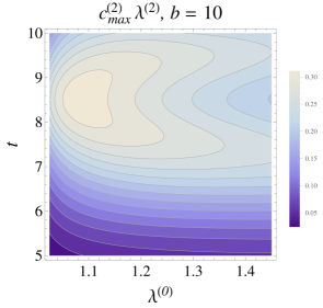
(a)

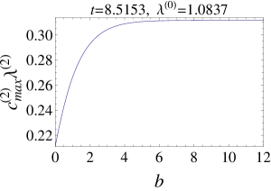
(b)

Figure 3: (a) Length of the interval $S^{(2)}=c^{(2)}_{max}\lambda^{(2)}$ over the $(\lambda_{0},t)$-plane at $b=10$. Maximum $S^{(2)}_{max}=0.3117$ corresponds to $t_{opt}=8.5153$, $\lambda^{(0)}_{opt}=1.0837$, $\lambda^{(2)}_{opt}=0.8960$. (b) The length of the interval $S^{(2)}$ as a function of $b$ at $t=t_{opt}$ and $\lambda=\lambda^{(0)}_{opt}$.

Finally, we construct the vector $X^{(0)}_{opt}$ corresponding to the above optimal values $t_{opt}$, $b_{opt}$ and $\lambda^{(0)}_{opt}$:

$$X^{(0)}_{opt}=\left(\begin{array}[]{c}0.40596\cr 0.15131\cr 0.14467\cr 0.00010i\cr-0.00010i\end{array}\right).$$ (86)

Case 2: $\lambda^{(1)}\neq\lambda^{(2)}$, $c^{(1)}\neq 0$, $c^{(2)}=0$.

Now the parameter $c^{(1)}$ must provide the non-negativity for the density matrix $\rho^{(S)}(0)$. Similar to $S^{(2)}$ in Sec.IV.3.1, $S^{(1)}$ is an increasing function of $b$, so its maximum corresponds to $b=b_{opt}\to\infty$. Again we set $b_{opt}=10$ and depicture $S^{(1)}=c^{(1)}_{max}\lambda^{(1)}$ as a function of $\lambda^{(0)}$ and $t$ at $b=10$ in Fig.4a. Next we find $t_{opt}$ and $\lambda^{(0)}_{opt}$ which maximize $S^{(1)}$: $S^{(1)}_{max}=0.2870$ at $t_{opt}=5.0326$ and $\lambda^{(0)}_{opt}=1.2201$. In addition, $\lambda^{(1)}_{opt}=0.8145$. For the optimal values $\lambda^{(0)}_{opt}$ and $t_{opt}$, the length of the interval $S^{(1)}$ as a function of $b$ is shown in Fig.4b.

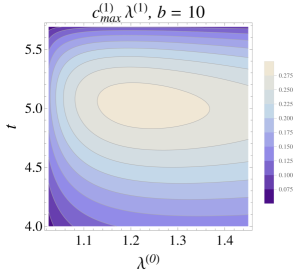
(a)

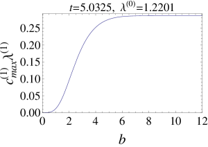
(b)

Figure 4: (a) Length of the interval $S^{(1)}=c^{(1)}_{max}\lambda^{(1)}$ over the $(\lambda_{0},t)$-plane at $b=10$. Maximum $S^{(1)}_{max}=0.2870$ corresponds to $t_{opt}=5.0326$, $\lambda^{(0)}_{opt}=1.2201$, $\lambda^{(1)}_{opt}=0.8145$. (b) Length of the interval $S^{(1)}=c^{(1)}_{max}\lambda^{(1)}$ as a function of $b$ at $\lambda^{(0)}_{opt}$ and $t_{opt}$.

Finally, we construct the vectors $X^{(0)}_{opt}$ and $X^{(1)}_{opt}$ corresponding to the above optimal values $t_{opt}$, $b_{opt}$ and $\lambda^{(0)}_{opt}$:

$$X^{(0)}_{opt}=\left(\begin{array}[]{c}0.59440\cr 0.12890\cr 0.09232\cr-0.10707i\cr 0.10707i\end{array}\right),\;\;X^{(1)}_{opt}=\left(\begin{array}[]{c}0.77790\cr-0.62839i\cr-0.00003i\cr-0.00004\end{array}\right).$$ (96)

Case 3: $\lambda^{(1)}\neq\lambda^{(2)}$, $c^{(1)}\neq 0$, $c^{(2)}\neq 0$.

Now the two parameters $c^{(1)}$ and $c^{(2)}$ must provide the nonnegativity for the density matrix $\rho^{(S)}(0)$. The maximum of the estimated area $S^{(12)}=c^{(1)}_{opt}c^{(2)}_{opt}\lambda^{(1)}_{opt}\lambda^{(2)}_{opt}=0.0189$ corresponds to $t_{opt}=5.3768$, $b_{opt}=5.3790$, $\lambda^{(0)}_{opt}=1.2634$, in addition $\lambda^{(1)}_{opt}=0.7613$ and $\lambda^{(2)}_{opt}=0.2289$. The estimated area $S^{(12)}$ as a function of $\lambda^{(0)}$ and $t$ at $b=b_{opt}$ is depicted in Fig.5a, while $S^{(12)}$ as a function of $b$ at $\lambda^{(0)}_{opt}$ and $t_{opt}$ is shown in Fig.5b. The semi-axes of the ellipse-like region are $S^{(1)}_{max}=c^{(1)}_{opt}\lambda^{(1)}_{opt}=0.2448$ and $S^{(2)}_{max}=c^{(2)}_{opt}\lambda^{(2)}_{opt}=0.0771$.

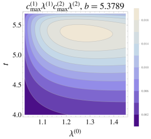
(a)

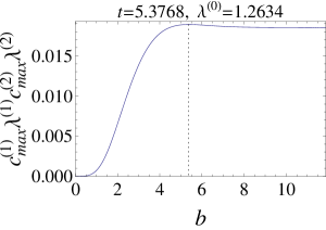
(b)

Figure 5: (a) The estimated area $S^{(12)}=c^{(1)}_{max}c^{(2)}_{max}\lambda^{(1)}\lambda^{(2)}$ over the $(\lambda_{0},t)$-plane at $b_{opt}=5.3790$. The maximum $S^{(12)}_{max}=0.0189$ corresponds to $t_{opt}=5.3768$, $\lambda^{(0)}_{opt}=1.2634$, $\lambda^{(1)}_{opt}=0.7613$, $\lambda^{(2)}_{opt}=0.2289$. (b) The estimated area $S^{(12)}$ as a function of $b$ at $\lambda^{(0)}_{opt}$ and $t_{opt}$. There is a maximum at $b=5.3789$.

Finally, we construct the vectors $X^{(0)}_{opt}$ and $X^{(1)}_{opt}$ corresponding to the above optimal values $t_{opt}$, $b_{opt}$ and $\lambda^{(0)}_{opt}$:

$$X^{(0)}_{opt}=\left(\begin{array}[]{c}0.51945\cr 0.18237\cr 0.07949\cr-0.11342i\cr 0.11342i\end{array}\right),\;\;X^{(1)}_{opt}=\left(\begin{array}[]{c}0.88361\cr-0.46820i\cr-0.00216i\cr-0.00408\end{array}\right).$$ (106)

Case 4: $\lambda^{(1)}=\lambda^{(2)}$, $c^{(1)}\neq 0$, $c^{(2)}\neq 0$.

At last, we can consider the case of uniform scaling of the higher-order coherence matrices (9):

$$\lambda^{(2)}=\lambda^{(1)}=\lambda.$$ (107)

The graph of the parameter $\lambda$ over the $(b,t)$-plane forms the curve shown in Fig.6.

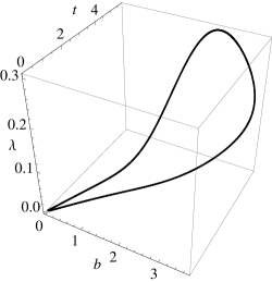
Figure 6: The parameter $\lambda$ over the plane $(b,t)$.

Again, the parameters $c^{(1)}$ and $c^{(2)}$ provide non-negativity for the density matrix $\rho^{(S)}(0)$. Similar to Sec.IV.3.1, the creatable region can be characterized by the estimated area $S^{(12)}$. This parameter is depicted in Fig.7 as a function of points $(b,t)$ satisfying condition (107) (i.e., the points of the projection of the curve in Fig.6 onto the plane $(b,t)$) for three values of $\lambda^{(0)}$: $\lambda^{(0)}=1$, $1.2022$, $1.4$. The maximum $S^{(12)}_{max}=0.0086$, corresponds to $b_{opt}=2.3462$, $t_{opt}=5.6651$, $\lambda^{(0)}_{opt}=1.2022$ with $\lambda_{opt}=0.2956$. The semi-axes are $S^{(1)}_{max}=c^{(1)}_{opt}\lambda_{opt}=0.0904$, $S^{(2)}_{max}=c^{(2)}_{opt}\lambda_{opt}=0.0946$.

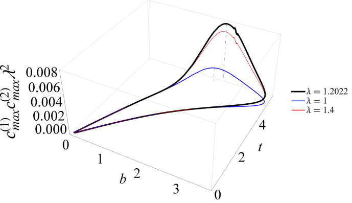
Figure 7: The estimated area $S^{(12)}=c^{(1)}_{max}c^{(2)}_{max}\lambda^{2}$ as a function of the point $(b,t)$ on the curve in Fig.6 at three values of the parameter $\lambda^{(0)}$: $\lambda^{(0)}=\lambda^{(0)}_{opt}=1.2022$, $\lambda^{(0)}=1.4>\lambda^{(0)}_{opt}$ and $\lambda^{(0)}=1<\lambda^{(0)}_{opt}$. Dash lines indicate the positions of the maxima.

Finally, the vectors $X^{(0)}_{opt}$ and $X^{(1)}_{opt}$ corresponding to the above optimal values $t_{opt}$, $b_{opt}$ and $\lambda^{(0)}_{opt}$ read:

$$X^{(0)}_{opt}=\left(\begin{array}[]{c}0.49962\cr 0.20645\cr 0.08884\cr-0.07298i\cr 0.07298i\end{array}\right),\;\;X^{(1)}_{opt}=\left(\begin{array}[]{c}0.98333\cr-0.15484i\cr-0.01482i\cr-0.09414\end{array}\right).$$ (117)

IV.3.2 Optimization of block-scaled state over $t$ and $b$ with $\lambda^{(0)}=1$ (perfect transfer of zero-order coherence matrix)

Unlike the higher order coherences, the zero-order coherence matrix can be perfectly transferred from the sender to the receiver, i.e., we can set $\lambda^{(0)}=1$ in map (43). It is likely that this possibility is associated with the classical nature of this coherence. Thus, the problem of state-restoring at the receiver side reduces to the operations with higher-order coherence matrices which encode the quantum information of the transferred state.

In this section, we consider the Cases 1-4 of Sec.IV.2 and perform the optimization of the creatable regions in the receiver’s state space setting $\lambda^{(0)}=1$. In all considered cases, the creatable region is smaller in comparison with the corresponding cases of Sec.IV.2. The brief results of optimization are below.

Case 1: $c^{(1)}=0$, $c^{(2)}\neq 0$.

In this case $t_{opt}=8.5153$, $b_{opt}=0$, $\lambda^{(2)}_{opt}=0.8960$ and the maximum of $S^{(2)}$ is $S^{(2)}_{max}=0.2240$, which is smaller in comparison with the same parameter in Sec.IV.3.1. The graph of $S^{(2)}$ as a function of $b$ at $t_{opt}$ is given in Fig.8a.

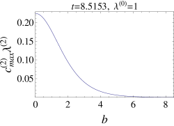
(a)

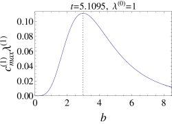
(b)

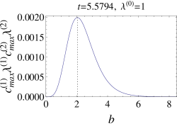
(c)

Figure 8: (a) Case 1: $S^{(2)}{=c^{(2)}_{max}\lambda^{(2)}}$ as a function of $b$ at $t_{opt}=8.5153$; (b) Case 2: $S^{(1)}{=c^{(1)}_{max}\lambda^{(1)}}$ as a function of $b$ at $t_{opt}=5.1095$; (c) Case 3: $S^{(12)}{=c^{(1)}_{max}\lambda^{(1)}c^{(2)}_{max}\lambda^{(2)}}$ as a function of $b$ at $t_{opt}=5.5794$.

The appropriate vector $X^{(0)}_{opt}$ corresponding to the above optimal values $t_{opt}$ and $b_{opt}$ is

$$X^{(0)}_{opt}=\left(\begin{array}[]{c}0.25\cr 0.25\cr 0.25\cr 0\cr 0\end{array}\right),$$ (123)

which corresponds to the zero-order coherence matrix in the form of the density matrix for the maximally mixed state.

Case 2: $c^{(1)}\neq 0$, $c^{(2)}=0$.

In this case $t_{opt}=5.1095$, $b_{opt}=2.9830$, $\lambda^{(1)}_{opt}=0.5444$ and the maximum of $S^{(1)}$ is $S^{(1)}_{max}=0.1111$, which is smaller in comparison with the same parameter in Sec.IV.3.1. The graph of $S^{(1)}$ as a function of $b$ at $t_{opt}$ is given in Fig.8b. The appropriate vectors $X^{(0)}_{opt}$ and $X^{(1)}_{opt}$ corresponding to the above optimal values $t_{opt}$ and $b_{opt}$ are

$$X^{(0)}_{opt}=\left(\begin{array}[]{c}0.90593\cr 0.04588\cr 0.04588\cr 0\cr 0\end{array}\right),\;\;X^{(1)}_{opt}=\left(\begin{array}[]{c}0.79903\cr-0.59916i\cr-0.03034i\cr-0.04046\end{array}\right).$$ (133)

Case 3: $c^{(1)}\neq 0$, $c^{(2)}\neq 0$.

In this case $t_{opt}=5.5794$, $b_{opt}=2.0412$, $\lambda^{(1)}_{opt}=0.2507$, $\lambda^{(2)}_{opt}=0.2748$ and the maximum of $S^{(12)}$ is $S^{(12)}_{max}=0.0020$, which is smaller in comparison with the same parameter in Sec.IV.3.1. The lengths of the semi-axes are $S^{(1)}_{max}=c^{(1)}_{opt}\lambda^{(1)}_{opt}=0.0713$, $S^{(2)}_{max}=c^{(2)}_{opt}\lambda^{(2)}_{opt}=0.0280$. The graph of $S^{(12)}$ as a function of $b$ at $t_{opt}$ is given in Fig.8c. The appropriate vectors $X^{(0)}_{opt}$ and $X^{(1)}_{opt}$ corresponding to the above optimal values $t_{opt}$ and $b_{opt}$ are

$$X^{(0)}_{opt}=\left(\begin{array}[]{c}0.78332\cr 0.10173\cr 0.10173\cr 0\cr 0\end{array}\right),\;\;X^{(1)}_{opt}=\left(\begin{array}[]{c}0.94716\cr-0.29378i\cr-0.03815i\cr-0.12301\end{array}\right).$$ (143)

Case 4: $\lambda^{(1)}=\lambda^{(2)}$, $c^{(1)}\neq 0$, $c^{(2)}\neq 0$.

In this case $t_{opt}=5.5574$, $b_{opt}=2.0950$, $\lambda_{opt}=0.2696$. Then, the maximum of $S^{(12)}$ is $S^{(12)}_{max}=0.00199$, which is smaller then the same parameter in Sec.IV.3.1. The lengths of the semi-axes are $S^{(1)}_{max}=c^{(1)}_{opt}\lambda_{opt}=0.0756$, $S^{(2)}_{max}=c^{(2)}_{opt}\lambda_{opt}=0.0263$. Thus, we see that the creatable region is smaller then the one obtained in Sec.IV.3.1. The graph of $S^{(12)}$ as a function of the points $(b,t)$ on the projection of the curve in Fig.6 onto the plane $(b,t)$ is given in Fig.7, the lower curve. The appropriate vectors $X^{(0)}_{opt}$ and $X^{(1)}_{opt}$ corresponding to the above optimal values $t_{opt}$ and $b_{opt}$ are

$$X^{(0)}_{opt}=\left(\begin{array}[]{c}0.79285\cr 0.09757\cr 0.09757\cr 0\cr 0\end{array}\right),\;\;X^{(1)}_{opt}=\left(\begin{array}[]{c}0.93988\cr-0.31891i\cr-0.03925i\cr-0.11567\end{array}\right).$$ (153)

IV.4 Creation of scaled coherence matrices in chain of $N=42$ nodes. Brief results

In these section we briefly repeat the results of Sec.IV.3 on creating the scaled coherence matrices in longer chain of $N=42$ nodes. In particular we do not provide the vectors $X^{(1)}$ and $X^{(0)}$ corresponding the optimal values of $t$, $b$ and $\lambda^{(0)}$.

IV.4.1 Optimization of block-scaled state over $\lambda^{(0)}$, $t$ and $b$

Case 1: $\lambda^{(1)}\neq\lambda^{(2)}$, $c^{(1)}=0$, $c^{(2)}\neq 0$.

The optimization shows that the maximum of $S^{(2)}$ corresponds to $b=b_{opt}\to\infty$ (similar to Sec.IV.3.1, we set $b_{opt}=10$). We have: $S^{(2)}_{max}=0.1146$ and $\lambda^{(2)}_{opt}=0.2620$ at $t_{opt}=47.9719$ and $\lambda^{(0)}_{opt}=1.6975$.

Case 2: $\lambda^{(1)}\neq\lambda^{(2)}$, $c^{(1)}\neq 0$, $c^{(2)}=0$.

We have $S^{(1)}_{max}=0.0468$ and $\lambda^{(1)}_{opt}=0.3187$ at $b_{opt}=7.0248$, $t_{opt}=41.3281$ and $\lambda^{(0)}_{opt}=1.3694$.

Case 3: $\lambda^{(1)}\neq\lambda^{(2)}$, $c^{(1)}\neq 0$, $c^{(2)}\neq 0$.

We have $S^{(12)}_{max}=c^{(1)}_{opt}c^{(2)}_{opt}\lambda^{(1)}_{opt}\lambda^{(2)}_{opt}=0.0007$, $\lambda^{(1)}_{opt}=0.2952$ and $\lambda^{(2)}_{opt}=0.0393$ at $b_{opt}=6.8796$, $t_{opt}=41.9410$, $\lambda^{(0)}_{opt}=1.5323$. The semi-axes of the optimized creatable region are $S^{(1)}_{max}=0.0390$ and $S^{(2)}_{max}=0.0178$.

Case 4: $\lambda^{(1)}=\lambda^{(2)}$, $c^{(1)}\neq 0$, $c^{(2)}\neq 0$.

Finally, we can consider the case of uniform scaling of the higher-order coherence matrices (9): $\lambda^{(2)}=\lambda^{(1)}=\lambda.$ We have $S^{(12)}_{max}=1.8720\times 10^{-4}$ and $\lambda_{opt}=0.0494$ at $b_{opt}=3.8922$, $t_{opt}=42.3077$, $\lambda^{(0)}_{opt}=1.4258$. The semi-axes of the optimized creatable region are $S^{(1)}_{max}=0.0088$ $S^{(2)}_{max}=0.0212$.

IV.4.2 Optimization of block-scaled state over $t$ and $b$ with $\lambda^{(0)}=1$ (perfect transfer of zero-order coherence matrix)

Case 1: $c^{(1)}=0$, $c^{(2)}\neq 0$.

We have $S^{(2)}_{max}=0.0655$ and $\lambda^{(2)}_{opt}=0.2621$ at $t_{opt}=47.8855$, $b_{opt}=0$.

Case 2: $c^{(1)}\neq 0$, $c^{(2)}=0$.

We have $S^{(1)}_{max}=0.0162$ and $\lambda^{(1)}_{opt}=0.2101$ at $t_{opt}=41.3423$, $b_{opt}=5.0997$.

Case 3: $c^{(1)}\neq 0$, $c^{(2)}\neq 0$.

We have $S^{(12)}_{max}=7.0609\times 10^{-6}$, $\lambda^{(1)}_{opt}=0.0699$ and $\lambda^{(2)}_{opt}=0.0454$ at $t_{opt}=42.1667$, $b_{opt}=4.0247$. The semi-axes of the optimized creatable region are $S^{(1)}_{max}=0.0090$, $S^{(2)}_{max}=0.0008$.

Case 4: $\lambda^{(1)}=\lambda^{(2)}$, $c^{(1)}\neq 0$, $c^{(2)}\neq 0$.

We have $S^{(12)}_{max}=6.7468\times 10^{-6}$ and $\lambda_{opt}=0.0473$ at $t_{opt}=42.2365$, $b_{opt}=3.8124$. The semi-axes of the optimized creatable region are $S^{(1)}_{max}=0.0067$, $S^{(2)}_{max}=0.0010$.

IV.5 Summary of results for chains of $N=6$ and $N=42$ nodes

Now we summarize the results characterizing the creatable regions in all cases considered in Secs.IV.3 and IV.4. The most important are the creatable intervals $S^{(1)}_{max}$ (Case 1), $S^{(2)}_{max}$ (Case 2) and areas $S^{(12)}_{max}=S^{(1)}_{max}S^{(2)}_{max}$ (Cases 3 and 4), as well as the scale factors $\lambda^{(1)}_{opt}$ and $\lambda^{(2)}_{opt}$. All these parameters are collected in Table 1 for the chains of 6 and 42 nodes.

Case $\#$	$N=6$				$N=42$
	$S^{(1)}_{max}$	$S^{(2)}_{max}$	$\lambda^{(1)}_{opt}$	$\lambda^{(2)}_{opt}$	$S^{(1)}_{max}$	$S^{(2)}_{max}$	$\lambda^{(1)}_{opt}$	$\lambda^{(2)}_{opt}$
Case 1	–	0.3117	–	0.8960	–	0.1146	–	0.2620
Case 2	0.2870	–	0.8145	–	0.0468	–	0.3187	–
Case 3	0.2448	0.0771	0.7613	0.2289	0.0390	0.0178	0.2952	0.0393
Case 4	0.0904	0.0946	0.2956	0.2956	0.0088	0.0212	0.0494	0.0494

(a) The optimized scale factor $\lambda^{(0)}=\lambda^{(0)}_{opt}$.

Case $\#$	$N=6$				$N=42$
	$S^{(1)}_{max}$	$S^{(2)}_{max}$	$\lambda^{(1)}_{opt}$	$\lambda^{(2)}_{opt}$	$S^{(1)}_{max}$	$S^{(2)}_{max}$	$\lambda^{(1)}_{opt}$	$\lambda^{(2)}_{opt}$
Case 1	–	0.2240	–	0.8960	–	0.0655	–	0.2621
Case 2	0.1111	–	0.5444	–	0.0162	–	0.2101	–
Case 3	0.0713	0.0280	0.2507	0.2748	0.0090	0.0008	0.0699	0.0454
Case 4	0.0756	0.0263	0.2696	0.2696	0.0067	0.0010	0.0473	0.0473

(b) The fixed scale factor $\lambda^{(0)}=1$.

Table 1: The semi-axes $S^{(1)}_{max}$ and $S^{(2)}_{max}$ of creatable regions and corresponding scale factors $\lambda^{(1)}_{opt}$ and $\lambda^{(2)}_{opt}$ for the chains of $N=6$ and 42 nodes.

This table shows us that the parameters $S^{(i)}_{max}$ and scale factors $\lambda^{(i)}_{opt}$ are bigger if we optimize $t$, $b$ and $\lambda^{(0)}$ for only one of the semi-axes, either $S^{(1)}$ or $S^{(2)}$. Simultaneous optimization for both of them reduces these parameters. Comparing Cases 3 and 4, we conclude that the creatable area reduces if we require equal scale factors $\lambda^{(1)}=\lambda^{(2)}=\lambda$ (although $S^{(2)}$ becomes slightly bigger in this case, except Table 1b, $N=6$). In this case, the scale factor $\lambda^{(1)}_{opt}$ is also less then $\max(\lambda^{(1)}_{opt},\lambda^{(2)}_{opt})$ in the case $\lambda^{(1)}\neq\lambda^{(2)}$. Another reducing factor is the requirement for the perfect transfer of the zero-order coherence matrix ($\lambda^{(0)}=1$), compare Table 1a and Table 1b. Finally, a crucial factor is the chain length $N$, which follows from comparing two columns $N=6$ and $N=42$ in Table 1. However, the later can be partially overcame using the optimization technique, such as optimizing boundary coupling constants BACVV2010 ; ZO ; BACVV2011 ; ABCVV ; SAOZ .

We emphasize that $\lambda^{(i)}_{opt}<1$ ($i=1,2$) and $\lambda^{(0)}_{opt}>1$, which holds in all our experiments (except the case of perfect zero order coherence transfer when $\lambda^{(0)}=1$ by our requirement). Thus, scaling of the higher-order coherence matrices is compressive, while scaling of the zero-order coherence matrix is stretching. Perhaps this difference is associated with the classical contribution to the zero-order coherence from the diagonal elements of the density matrix.

V Conclusion

The problem of manipulating the quantum information distribution in a quantum communication line is of principal importance. A well known method of an ideal manipulation is the perfect state transfer allowing to transfer multi-qubit states (up to the mirror symmetry) without any deformation. However, this ideal transfer is hardly realizable in practice because it requires very special properties of a communication line. In practice, during evolution the state experiences dispersion and decay which result in mixing all elements of the transferred density matrix. In particular, if the sender’s initial state was a pure one, it becomes a mixed state at the receiver side.

Therefore, the development of another ways of information propagation is an important and still unresolved problem. We propose the information propagation using the states that can be transferred with a minimal deformation. This deformation can be simply described as scaling the matrix elements without mixing them and, which is important, our protocol is not sensitive to the particular realization of a communication line. The only requirement for the Hamiltonian is preserving the excitation number in a quantum system.

In this paper, we do not apply any additional tools to prevent mixing matrix elements. Thus, the evolution of the sender’s initial density matrix without mixing its elements is provided by its particular structure. We find states such that the scale factors of all elements inside of each block are the same (except for the only diagonal element which fixes the normalization). We call the states evolving in this way the block-scaled states.

In our case, the scaling of higher order MQ-coherence matrices is compressive ($|\lambda^{(i)}|<1$, $i=1,2$). This is a consequence of the dispersion which supplements the evolution. On the contrary, the scaling of zero-order coherence matrix (without a single diagonal element which must satisfy the normalization condition) can be stretching ($\lambda^{(0)}\geq 1$ in all our examples). Eventually, the scale factors of higher order coherence matrices tend to zero as $t\to\infty$. Consequently, the information (both classical and quantum) survives in the zero-order coherence matrix in this limit.

The presence of a free parameter in each MQ-coherence matrix (respectively, $\lambda^{(0)}$, $c^{(1)}$ and $c^{(2)}$) might be enough to establish the full control of coherence intensities inside of the bounded region of their available values. To control all elements of transferred coherence matrices, an extension of this protocol to introduce more free parameters in the transferred state is required. A possible strategy in this direction is implementing the unitary-transformation tool at the receiver side FZ_2017 .

The found states which evolve to the block-scaled states can serve for the distribution of quantum information in a communication line.

Finally, we give several remarks regarding the features of the proposed protocol.

1. Admissible values of parameters $\lambda^{(0)}$, $c^{(1)}$ and $c^{(2)}$ provide the non-negativity for the transferred density matrix, so that they cover a bounded region in the three dimensional space of these parameters.

2. Although the quantum effects prevail at low temperature ($b\to\infty$), the optimal values of $b$ in many our examples are finite (see Secs.IV.3.1, IV.3.1, IV.3.2). Perhaps, this means the presence of combined classical-quantum contribution into the corresponding process.

3. The zero-order coherence matrices of certain sender states can be perfectly transferred to the receiver, while this is impossible for the higher-order coherence matrix. Perhaps, this is because the zero-order coherence includes the diagonal elements of the density matrix which are responsible for the classical correlations. States possessing this property are the least structurally deformed in comparison with other block-scaled states.

4. The block-scale transfer is not related to the particular geometry of a communication line, so that there is a large freedom in realization of this protocol. The only requirement for the Hamiltonian is conserving the excitation number in the spin system. This implies the option of splitting the density matrix into the set of MQ-coherence matrices which do not mix with each other during evolution.

5. The result of remote block-scaled state-creation depends on the parity of the spin chain. In particular, there is a cyclic dependence of the phase of the scale factors $\lambda^{(i)}$, $i=1,2$, on the chain length $N$. A consequence of this dependence is that the uniform scaling $\lambda^{(1)}=\lambda^{(2)}$ can be established only in the chains of $N=2+4n$ ($n\in{\mathbb{N}}$) nodes.

This work is partially supported by the program of the Presidium of RAS No. 5 ”Electron resonance, spin-dependent electron effects and spin technology” and by the Russian Foundation for Basic Research (Grants No.15-07-07928, No.16-03-00056).

VI Appendix. Derivation of receiver density matrix

VI.1 Jordan-Wigner transformation

First, we recall some basic formulas of the Jordan-Wigner transformation JW ; CG . The operators $I^{\pm}_{n}=I_{xn}\pm iI_{yn}$ generate the fermion operators $c_{n}$ and $c_{n}^{+}$ by the formulas:

$$c_{j}=(-2)^{j-1}\prod_{i=1}^{j-1}I_{zi}I_{j}^{-},\;\;c_{j}^{+}=(-2)^{j-1}\prod_{i=1}^{j-1}I_{zi}I_{j}^{+},$$ (154)

which satisfy the anti-commutation relations

$$\{c_{j},c_{i}\}=0,\;\;\{c_{j}^{+},c_{i}^{+}\}=0,\;\;\{c_{j}^{+},c_{i}\}=\delta_{ij},$$ (155)

therefore $I_{zj}=c_{j}^{+}c_{j}-\frac{1}{2}$. We also introduce the operators $\beta_{n}$ as Fourier transforms of $c_{n}$:

$$c_{j}=\sum_{k=1}^{N}g_{jk}\beta_{k},\;\;g_{kj}=\left(\frac{2}{N+1}\right)^{1/2}\sin\frac{\pi kj}{N+1},$$ (156)

Then, the Hamiltonian (4) in terms of the operators $\beta_{n}$ reads:

$$H=\sum_{k=1}^{N}\varepsilon_{k}\beta_{k}^{+}\beta_{k},\;\;\varepsilon_{k}=\cos\frac{\pi k}{N+1}.$$ (157)

and therefore the following evident relations among the operators $I_{\alpha j}$ and $c_{j}$:

$$I_{zj}=c_{j}^{+}c_{j}-\frac{1}{2},\;\;I_{1}^{-}=c_{1},\;\;\;I_{1}^{+}=c_{1}^{+},\;\;\;I_{2}^{-}=-2I_{z1}c_{1},\;\;\;I_{2}^{+}=-2I_{z1}c_{1}^{+}.$$ (158)

VI.2 Evolution

Now we consider the evolution of the initial state $\rho(0)$ (11) and write it in the following form convenient for the further analytical calculations:

$$\rho(t)=\frac{1}{Z}e^{-itH}r_{0}e^{itH}e^{bI_{z}}=\frac{r(t)}{Z}e^{bI_{z}},\;\;r_{0}=\rho(0)e^{-bI_{z1}}e^{-bI_{z2}}.$$ (159)

For convenience we present $r_{0}$ in the basis of matrices $4\times 4$:

$$r_{0} = \tilde{a}_{00}E+\tilde{a}_{01}I_{z1}+\tilde{a}_{02}I_{z2}+\tilde{a}_{03}I_{z1}I_{z2}+\tilde{a}_{11}I_{2}^{-}+\tilde{a}_{12}I_{2}^{+}+\tilde{a}_{13}I_{z1}I_{2}^{-}+\tilde{a}_{14}I_{z1}I_{2}^{+}+$$

$$\tilde{a}_{15}I_{1}^{-}I_{2}^{+}+\tilde{a}_{16}I_{1}^{+}I_{2}^{-}+\tilde{a}_{21}I_{1}^{-}+\tilde{a}_{22}I_{1}^{+}+\tilde{a}_{23}I_{1}^{-}I_{z2}+\tilde{a}_{24}I_{1}^{+}I_{z2}+\tilde{a}_{31}I_{1}^{-}I_{2}^{-}+\tilde{a}_{32}I_{1}^{+}I_{2}^{+},$$

where $\tilde{a}_{ij}$ are explicitly given in terms of $a_{ij}$ in Eq.(IV):

$$\tilde{a}_{00}=\frac{1}{8}\Big{(}1-a_{03}+(1+a_{03})\cosh(b)-2(a_{01}+a_{02})\sinh(b)\Big{)},$$ (161)

$$\tilde{a}_{01}=\frac{1}{4}\Big{(}2(a_{01}-a_{02})+2(a_{01}+a_{02})\cosh(b)-(1+a_{03})\sinh(b)\Big{)},$$

$$\tilde{a}_{02}=\frac{1}{4}\Big{(}2(a_{02}-a_{01})+2(a_{01}+a_{02})\cosh(b)-(1+a_{03})\sinh(b)\Big{)},$$

$$\tilde{a}_{03}=\frac{1}{2}\Big{(}-1+a_{03}+(1+a_{03})\cosh(b)-2(a_{01}+a_{02})\sinh(b)\Big{)},$$

$$\tilde{a}_{11}=\frac{1}{4}\Big{(}2(e^{-b}+1)a_{11}+(e^{-b}-1)a_{12}\Big{)},\;\;\;$$

$$\tilde{a}_{12}=\frac{1}{4}\Big{(}2(e^{b}+1)a_{11}^{*}-(e^{b}-1)a_{12}^{*}\Big{)},\;\;\;$$

$$\tilde{a}_{13}=\frac{1}{2}\Big{(}2(e^{-b}-1)a_{11}+(e^{-b}+1)a_{12}\Big{)},$$

$$\tilde{a}_{14}=\frac{1}{2}\Big{(}-2(e^{b}-1)a_{11}^{*}+(e^{b}+1)a_{12}^{*}\Big{)},$$

$$\tilde{a}_{15}=a_{13},\;\;\tilde{a}_{16}=a_{13}^{*},$$

$$\tilde{a}_{21}=\frac{1}{4}\Big{(}2(e^{-b}+1)a_{21}+(e^{-b}-1)a_{22}\Big{)},\;\;\;$$

$$\tilde{a}_{22}=\frac{1}{4}\Big{(}2(e^{b}+1)a_{21}^{*}-(e^{b}-1)a_{22}^{*}\Big{)},\;\;\;$$

$$\tilde{a}_{23}=\frac{1}{2}\Big{(}2(e^{-b}-1)a_{21}+(e^{-b}+1)a_{22}\Big{)},$$

$$\tilde{a}_{24}=\frac{1}{2}\Big{(}-2(e^{b}-1)a_{21}^{*}+(e^{b}+1)a_{22}^{*}\Big{)},$$

$$\tilde{a}_{31}=e^{-b}a_{31},\;\;\tilde{a}_{32}=e^{b}a_{31}^{*},$$

The time dependence of the density matrix is embedded in the transition amplitudes:

$$f_{ij}=\sum_{k=1}^{N}g_{ik}g_{kj}e^{-it\varepsilon_{k}},\;\;i,j=N,N-1,$$ (162)

and the matrix $r(t)=e^{-itH}r_{0}e^{itH}$ in Eq.(159) can be given in the following form:

$$r(t)=A^{0}+\sum_{j}(A^{11}_{j}c_{j}+A^{12}_{j}c_{j}^{+})+\sum_{j_{1},j_{2}}(A^{21}_{j_{1}j_{2}}c_{j_{1}}^{+}c_{j_{2}}+A^{22}_{j_{1}j_{2}}c_{j_{1}}c_{j_{2}}+A^{23}_{j_{1}j_{2}}c_{j_{1}}^{+}c_{j_{2}}^{+})+$$ (163)

$$\sum_{j_{1},j_{2},j_{3}}(A^{31}_{j_{1}j_{2}j_{3}}c_{j_{1}}^{+}c_{j_{2}}c_{j_{3}}+A^{32}_{j_{1}j_{2}j_{3}}c_{j_{1}}^{+}c_{j_{2}}^{+}c_{j_{3}})+\sum_{j_{1},j_{2},j_{3},j_{4}}A^{41}_{j_{1}j_{2}j_{3}j_{4}}c_{j_{1}}^{+}c_{j_{2}}^{+}c_{j_{3}}c_{j_{4}}$$

where

$$A^{0}=\tilde{a}_{00}-\frac{\tilde{a}_{01}}{2}-\frac{\tilde{a}_{02}}{2}+\frac{\tilde{a}_{03}}{4},$$ (164)

$$A^{11}_{j}=(\tilde{a}_{11}-\frac{\tilde{a}_{13}}{2})f_{2j}^{*}+(\tilde{a}_{21}-\frac{\tilde{a}_{23}}{2})f_{1j}^{*},\;\;A^{12}_{j}=(\tilde{a}_{12}-\frac{\tilde{a}_{14}}{2})f_{2j}+(\tilde{a}_{22}-\frac{\tilde{a}_{24}}{2})f_{1j},$$

$$A^{21}_{j_{1}j_{2}}=(\tilde{a}_{01}-\frac{\tilde{a}_{03}}{2})f_{1j_{1}}f_{1j2}^{*}+(\tilde{a}_{02}-\frac{\tilde{a}_{03}}{2})f_{2j_{1}}f_{2j2}^{*}+\tilde{a}_{15}f_{2j_{1}}f_{1j_{2}}^{*}+\tilde{a}_{16}f_{1j_{1}}f_{2j_{2}}^{*},$$

$$A^{21}_{0}=\sum_{j=1}^{N}A^{21}_{jj}=\tilde{a}_{01}+\tilde{a}_{02}-\tilde{a}_{03},\;\;A^{22}_{j_{1}j_{2}}=-\tilde{a}_{31}f_{1j_{1}}^{*}f_{2j_{2}}^{*},\;\;A^{23}_{j_{1}j_{2}}=\tilde{a}_{32}f_{1j_{1}}f_{2j_{2}},$$

$$A^{31}_{j_{1}j_{2}j_{3}}=\tilde{a}_{23}f_{2j_{1}}f_{2j_{2}}^{*}f_{1j_{3}}^{*}-2\tilde{a}_{11}f_{1j_{1}}f_{1j_{2}}^{*}f_{2j_{3}}^{*},$$

$$A^{31}_{j_{2}}=\sum_{j=1}^{N}A^{31}_{jjj_{2}}=\tilde{a}_{23}f_{1j_{2}}^{*}-2\tilde{a}_{11}f_{2j_{2}}^{*},\;\;\sum_{j=1}^{N}A^{31}_{jj_{2}j}=0,$$

$$A^{32}_{j_{1}j_{2}j_{3}}=\tilde{a}_{24}f_{1j_{1}}f_{2j_{2}}f_{2j_{3}}^{*}-2\tilde{a}_{12}f_{2j_{1}}f_{1j_{2}}f_{1j_{3}}^{*},\;\;A^{32}_{j_{2}}=\sum_{j=1}^{N}A^{32}_{j_{2}jj}=\tilde{a}_{24}f_{1j_{2}}-2\tilde{a}_{12}f_{2j_{2}},$$

$$\sum_{j=1}^{N}A^{32}_{jj_{2}j}=0,\;\;A^{41}_{j_{1}j_{2}j_{3}j_{4}}=-\tilde{a}_{03}f_{1j_{1}}f_{2j_{2}}f_{1j_{3}}^{*}f_{2j_{4}}^{*},,$$

$$A^{41;1}_{j_{2}j_{3}}=\sum_{j=1}^{N}A^{41}_{jj_{2}jj_{3}}=-\tilde{a}_{03}f_{2j_{2}}f_{2j_{3}}^{*},\;\;A^{41;2}_{j_{2}j_{3}}=\sum_{j=1}^{N}A^{41}_{j_{2}jj_{3}j}=-\tilde{a}_{03}f_{1j_{2}}f_{1j_{3}}^{*},\;\;$$

$$\sum_{j=1}^{N}A^{41}_{jj_{2}j_{3}j}=\sum_{j=1}^{N}A^{41}_{j_{2}jjj_{3}}=0,\;\;A^{41}_{0}=\sum_{j_{1},j_{2}=1}^{N}A^{41}_{j_{1}j_{2}j_{1}j_{2}}=-\tilde{a}_{03}.$$

VI.3 Reduced density matrix

Now we construct the reduced density matrix $\rho^{(R)}$ describing the receiver state,

$$\rho^{(R)}=Tr_{/R}\rho(t)=\frac{1}{Z}\tilde{\rho}_{0}(t)e^{bI_{z}},$$ (165)

calculating the trace of each term in expression (159). For the elements of this density matrix we have the formulas (38-40) with the following relations between $\rho^{(S)}_{ij}$ and $a_{ij}$:

$$\rho^{(S)}_{11}=\frac{1}{4}(1+2a_{01}+2a_{02}+a_{03}),\;\;\rho^{(S)}_{12}=\frac{1}{2}(2a^{*}_{11}+a^{*}_{12}),\;\;\rho^{(S)}_{13}=\frac{1}{2}(2a^{*}_{21}+a^{*}_{22}),$$ (166)

$$\rho^{(S)}_{14}=a^{*}_{31},\;\;\rho^{(S)}_{22}=\frac{1}{4}(1+2a_{01}-2a_{02}-a_{03}),\;\;\rho^{(S)}_{23}=a^{*}_{13},\;\;\rho^{(S)}_{24}=\frac{1}{2}(2a^{*}_{21}-a^{*}_{22}),$$

$$\rho^{(S)}_{33}=\frac{1}{4}(1-2a_{01}+2a_{02}-a_{03}),\;\;\rho^{(S)}_{34}=\frac{1}{2}(2a^{*}_{11}-a^{*}_{12}),\;\;\rho^{(S)}_{44}=1-\sum_{n=1}^{3}\rho^{(S)}_{nn}.$$

In addition, the coefficients $\alpha_{ij;nm}$ in the formulas (38)-(40) for the elements of the density matrix $\rho^{(R)}$ are given by the following expressions:

$$\alpha_{11,11}=K_{1}^{2}(e^{2b}+e^{b}\sum_{i=1}^{2}\sum_{j={N-1}}^{N}|f_{i,j}|^{2}+$$ (167)

$$(f_{1,N}f_{2,N-1}-f_{1,N-1}f_{2,N})(f_{1,N}^{*}f_{2,N-1}^{*}-f_{1,N-1}^{*}f_{2,N}^{*})),$$

$$\alpha_{11,22}=K_{2}(-(e^{b}+|f_{1,N}|^{2})(|f_{2,N-1}|^{2}-1)+$$ (168)

$$(-e^{b}f_{2,N}+f_{1,N}f_{2,N-1}f_{1,N-1}^{*})f_{2,N}^{*}+f_{1,N-1}(f_{2,N}f_{1,N}^{*}f_{2,N-1}^{*}+f_{1,N-1}^{*}(1-|f_{2,N}|^{2}))),$$

$$\alpha_{11,33}=K_{2}(e^{b}+|f_{2,N-1}|^{2}+|f_{2,N}|^{2}-$$ (169)

$$f_{1,N-1}(f_{1,N-1}^{*}(e^{b}+|f_{2,N}|^{2})-f_{2,N}f_{1,N}^{*}f_{2,N-1}^{*})-$$

$$f_{1,N}(e^{b}f_{1,N}^{*}+f_{2,N-1}(f_{1,N}^{*}f_{2,N-1}^{*}-f_{1,N-1}^{*}f_{2,N}^{*}))),$$

$$\alpha_{11,44}=K_{2}e^{b}((|f_{1,N}|^{2}-1)(|f_{2,N-1}|^{2}-1)-$$ (170)

$$(f_{2,N}+f_{1,N}f_{2,N-1}f_{1,N-1}^{*})f_{2,N}^{*}+f_{1,N-1}(f_{1,N-1}^{*}(|f_{2,N}|^{2}-1)-f_{2,N}f_{1,N}^{*}f_{2,N-1}^{*})),$$

$$\alpha_{11,23}=\alpha_{11,32}^{*}=K_{1}e^{b}(f_{1,N-1}f_{2,N-1}^{*}+f_{1,N}f_{2,N}^{*})$$ (171)

$$\alpha_{22,11}=K_{1}^{2}(-(|f_{1,N}|^{2}-1)(e^{b}+|f_{2,N-1}|^{2})+$$ (172)

$$(f_{1,N}f_{2,N-1}f_{1,N-1}^{*}-e^{b}f_{2,N})f_{2,N}^{*}+f_{1,N-1}(f_{2,N}f_{1,N}^{*}f_{2,N-1}^{*}+f_{1,N-1}^{*}(1-|f_{2,N}|^{2}))),$$

$$\alpha_{22,22}=K_{1}^{2}(e^{b}(|f_{1,N}|^{2}-1)(|f_{2,N-1}|^{2}-1)+$$ (173)

$$e^{b}(e^{b}f_{2,N}-f_{1,N}f_{2,N-1}f_{1,N-1}^{*})f_{2,N}^{*}+f_{1,N-1}(f_{1,N-1}^{*}(1+e^{b}|f_{2,N}|^{2})-e^{b}f_{2,N}f_{1,N}^{*}f_{2,N-1}^{*})),$$

$$\alpha_{22,33}=K_{1}^{2}(e^{b}+|f_{2,N-1}|^{2}+e^{b}(|f_{1,N}|^{2}(e^{b}+|f_{2,N-1}|^{2})-$$ (174)

$$(f_{2,N}+f_{1,N}f_{2,N-1}f_{1,N-1}^{*})f_{2,N}^{*}+f_{1,N-1}(f_{1,N-1}^{*}(|f_{2,N}|^{2}-1)-f_{2,N}f_{1,N}^{*}f_{2,N-1}^{*}))),$$

$$\alpha_{22,44}=K_{1}^{2}e^{b}(-(1+e^{b}|f_{1,N}|^{2})(|f_{2,N-1}|^{2}-1)+$$ (175)

$$e^{b}(f_{2,N}+f_{1,N}f_{2,N-1}f_{1,N-1}^{*})f_{2,N}^{*}-f_{1,N-1}(f_{1,N-1}^{*}(1+e^{b}|f_{2,N}|^{2})-e^{b}f_{2,N}f_{1,N}^{*}f_{2,N-1}^{*})),$$

$$\alpha_{22,23}=\alpha_{22,32}^{*}=K_{1}(f_{1,N-1}f_{2,N-1}^{*}-e^{b}f_{1,N}f_{2,N}^{*})$$ (176)

$$\alpha_{33,11}=K_{1}^{2}(e^{b}+|f_{1,N}|^{2}+|f_{2,N}|^{2}-f_{2,N-1}((e^{b}+|f_{1,N}|^{2})f_{2,N-1}^{*}-f_{1,N}f_{1,N-1}^{*}f_{2,N}^{*})-$$ (177)

$$f_{1,N-1}(f_{1,N-1}^{*}(e^{b}+|f_{2,N}|^{2})-f_{2,N}f_{1,N}^{*}f_{2,N-1}^{*})),$$

$$\alpha_{33,22}=K_{1}^{2}(e^{b}+|f_{1,N}|^{2}+e^{b}(-|f_{2,N}|^{2}+$$ (178)

$$f_{2,N-1}((e^{b}+|f_{1,N}|^{2})f_{2,N-1}^{*}-f_{1,N}f_{1,N-1}^{*}f_{2,N}^{*})+f_{1,N-1}(f_{1,N-1}^{*}(|f_{2,N}|^{2}-1)-f_{2,N}f_{1,N}^{*}f_{2,N-1}^{*}))),$$

$$\alpha_{33,33}=K_{1}^{2}(|f_{2,N}|^{2}+e^{b}((|f_{1,N}|^{2}-1)(|f_{2,N-1}|^{2}-1)-f_{1,N}f_{2,N-1}f_{1,N-1}^{*}f_{2,N}^{*})+$$ (179)

$$e^{b}f_{1,N-1}(f_{1,N-1}^{*}(e^{b}+|f_{2,N}|^{2})-f_{2,N}f_{1,N}^{*}f_{2,N-1}^{*})),$$

$$\alpha_{33,44}=-K_{2}(|f_{1,N}|^{2}+|f_{2,N}|^{2}-1+$$ (180)

$$e^{b}(f_{2,N-1}((|f_{1,N}|^{2}-1)f_{2,N-1}^{*}-f_{1,N}f_{1,N-1}^{*}f_{2,N}^{*})+f_{1,N-1}(f_{1,N-1}^{*}(|f_{2,N}|^{2}-1)-f_{2,N}f_{1,N}^{*}f_{2,N-1}^{*}))),$$

$$\alpha_{33,23}=\alpha_{33,32}^{*}=K_{1}(f_{1,N}f_{2,N}^{*}-e^{b}f_{1,N-1}f_{2,N-1}^{*})$$ (181)

$$\alpha_{23,11}=K_{1}(f_{1,N-1}f_{1,N}^{*}+f_{2,N-1}f_{2,N}^{*}),$$ (182)

$$\alpha_{23,22}=K_{1}f_{1,N-1}f_{1,N}^{*}-e^{b}f_{2,N-1}f_{2,N}^{*}),$$ (183)

$$\alpha_{23,33}=K_{1}f_{2,N-1}f_{2,N}^{*}-e^{b}f_{1,N-1}f_{1,N}^{*}),$$ (184)

$$\alpha_{23,44}=-K_{1}e^{b}(f_{1,N-1}f_{1,N}^{*}+f_{2,N-1}f_{2,N}^{*}),$$ (185)

$$\alpha_{23,23}=f_{1,N-1}f_{2,N}^{*},$$ (186)

$$\alpha_{23,32}=f_{2,N-1}f_{1,N}^{*}$$ (187)

$$\alpha_{12,12}=K_{3}(e^{b}f_{2,N}+(f_{1,N}f_{2,N-1}-f_{1,N-1}f_{2,N})f_{1,N-1}^{*}),$$ (188)

$$\alpha_{12,13}=-K_{3}(e^{b}f_{1,N}+(f_{1,N-1}f_{2,N}-f_{1,N}f_{2,N-1})f_{2,N-1}^{*}),$$ (189)

$$\alpha_{12,24}=K_{4}(f_{1,N}-(f_{1,N}f_{2,N-1}-f_{1,N-1}f_{2,N})f_{2,N-1}^{*}),$$ (190)

$$\alpha_{12,34}=K_{4}(f_{2,N}+(f_{1,N}f_{2,N-1}-f_{1,N-1}f_{2,N})f_{1,N-1}^{*})$$ (191)

$$\alpha_{13,12}=-K_{3}(f_{1,N-1}f_{2,N}f_{1,N}^{*}+f_{2,N-1}(e^{b}-|f_{1,N}|^{2})),$$ (192)

$$\alpha_{13,13}=K_{3}(f_{1,N}f_{2,N-1}f_{2,N}^{*}+f_{1,N-1}(e^{b}-|f_{2,N}|^{2})),$$ (193)

$$\alpha_{13,24}=K_{4}(f_{1,N-1}(|f_{2,N}|^{2}-1)-f_{1,N}f_{2,N-1}f_{2,N}^{*}),$$ (194)

$$\alpha_{13,34}=K_{4}(f_{2,N-1}(|f_{1,N}|^{2}-1)-f_{1,N-1}f_{2,N}f_{1,N}^{*})$$ (195)

$$\alpha_{24,12}=K_{3}(f_{2,N-1}(|f_{1,N}|^{2}-1)-f_{1,N-1}f_{2,N}f_{1,N}^{*}),$$ (196)

$$\alpha_{24,13}=K_{3}(f_{1,N}f_{2,N-1}f_{2,N}^{*}+f_{1,N-1}(1-|f_{2,N}|^{2})),$$ (197)

$$\alpha_{24,24}=-K_{3}(f_{1,N-1}+e^{b}(f_{1,N}f_{2,N-1}-f_{1,N-1}f_{2,N})f_{2,N}^{*}),$$ (198)

$$\alpha_{24,34}=-K_{3}(f_{2,N-1}+e^{b}(f_{1,N-1}f_{2,N}-f_{1,N}f_{2,N-1})f_{1,N}^{*})$$ (199)

$$\alpha_{34,12}=-K_{3}(f_{2,N}+(f_{1,N}f_{2,N-1}-f_{1,N-1}f_{2,N})f_{1,N-1}^{*}),$$ (200)

$$\alpha_{34,13}=K_{3}(f_{1,N}-(f_{1,N}f_{2,N-1}-f_{1,N-1}f_{2,N})f_{2,N-1}^{*}),$$ (201)

$$\alpha_{34,24}=K_{3}(e^{b}(f_{1,N}f_{2,N-1}-f_{1,N-1}f_{2,N})f_{2,N-1}^{*}-f_{1,N}),$$ (202)

$$\alpha_{34,34}=-K_{3}(e^{b}(f_{1,N}f_{2,N-1}-f_{1,N-1}f_{2,N})f_{1,N-1}^{*}+f_{2,N}),$$ (203)

$$\alpha_{14,14}=f_{1,N-1}f_{2,N}-f_{1,N}f_{2,N-1}$$ (204)

where

$$K_{1}=\frac{1}{1+e^{b}},\;\;K_{2}=\frac{1}{2(1+\cosh\;b)},$$ (205)

$$K_{3}=\frac{(-1)^{N}e^{-\frac{b}{2}}\tanh^{N-3}\frac{b}{2}}{2\cosh\frac{b}{2}},\;\;K_{4}=\frac{(-1)^{N}e^{\frac{b}{2}}\tanh^{N-3}\frac{b}{2}}{2\cosh\frac{b}{2}}.$$

References

- (1) S. Bose, Phys. Rev. Lett. 91, 207901 (2003)
- (2) M.Christandl, N.Datta, A.Ekert, and A.J.Landahl, Phys.Rev.Lett. 92, 187902 (2004)
- (3) C.Albanese, M.Christandl, N.Datta, and A.Ekert, Phys.Rev.Lett. 93, 230502 (2004)
- (4) P.Karbach and J.Stolze, Phys.Rev.A 72, 030301(R) (2005)
- (5) G.Gualdi, V.Kostak, I.Marzoli, and P.Tombesi, Phys.Rev. A 78, 022325 (2008)
- (6) A.Wójcik, T.Luczak, P.Kurzyński, A.Grudka, T.Gdala, and M.Bednarska Phys. Rev. A 72, 034303 (2005)
- (7) E.B.Fel’dman, E.I.Kuznetsova and A.I.Zenchuk, Phys. Rev. A 82, 022332 (2010)
- (8) L. Banchi, T. J. G. Apollaro, A. Cuccoli, R. Vaia, and P. Verrucchi, Phys.Rev.A 82, 052321 (2010)
- (9) A. Zwick and O. Osenda, J. Phys. A: Math. Theor. 44, (2011) 105302.
- (10) L. Banchi, T. J. G. Apollaro, A. Cuccoli, R. Vaia and P. Verrucchi, New J. Phys. 13, 123006 (2011)
- (11) T. J. G. Apollaro, L. Banchi, A. Cuccoli, R. Vaia, and P. Verrucchi, Phys. Rev. A 85 (2012), 052319
- (12) J.Stolze, G. A. Álvarez, O. Osenda, and A. Zwick in Quantum State Transfer and Network Engineering. Quantum Science and Technology, ed. by G.M.Nikolopoulos and I.Jex, Springer Berlin Heidelberg, Berlin, p.149 (2014)
- (13) N.A.Peters, J.T.Barreiro, M.E.Goggin, T.-C.Wei, and P.G.Kwiat, Phys.Rev.Lett. 94, 150502 (2005)
- (14) N.A.Peters, J.T.Barreiro, M.E.Goggin, T.-C.Wei, and P.G.Kwiat in Quantum Communications and Quantum Imaging III, ed. R.E.Meyers, Ya.Shih, Proc. of SPIE 5893 (SPIE, Bellingham, WA, 2005)
- (15) G.Y. Xiang, J.Li, B.Yu, and G.C.Guo Phys. Rev. A 72, 012315 (2005)
- (16) Liu, L.L., Hwang, T., Controlled remote state preparation protocols via AKLT states, Quantum Inf.Process. 13, 1639-1650 (2014)
- (17) A.I.Zenchuk, Phys. Rev. A 90, 052302(13) (2014)
- (18) G. A. Bochkin and A. I. Zenchuk, Phys.Rev.A 91, 062326(11) (2015)
- (19) G. Bochkin and A. Zenchuk, Extension of the remotely creatable region via the local unitary transformation on the receiver side, Quntum Information and Computation, 16 (2016) 1349-1364
- (20) E.B.Fel’dman , E. I. Kuznetsova, A.I.Zenchuk, Quantum Inf. Proc. 15 (2016) 2521
- (21) J.Stolze and A.I.Zenchuk, Quant. Inf. Proc. 15, (2016) 3347
- (22) E.B.Fel’dman, A.I.Zenchuk, JETP 125, 1042 (2017)
- (23) J. Baum, M. Munowitz, A. N. Garroway, and A. Pines, J. Chem. Phys. 83, 2015 (1985).
- (24) S. I. Doronin, I. I. Maksimov, and E. B. Fel’dman, J. Exp. Theor. Phys. 91, 597 (2000).
- (25) S. I. Doronin, E. B. Fel’dman, and A. I. Zenchuk, J.Chem.Phys. 134, 034102 (2011)
- (26) H.G. Krojanski and D. Suter, Phys. Rev. Lett. 93, 090501 (2004).
- (27) H.G. Krojanski and D. Suter, Phys. Rev. Lett. 97, 150503 (2006).
- (28) G. A. Alvarez and D. Suter, Phys. Rev. Lett. 104, 230403 (2010).
- (29) H.J. Cho, P. Cappellaro, D. G. Cory, and C. Ramanathan, Phys. Rev. B 74, 224434 (2006).
- (30) G.A.Bochkin, E.B.Fel’dman, S.G.Vasil’ev, V.I.Volkov, Chem.Phys.Lett. 680, 56 (2017).
- (31) P.Jordan, E.Wigner, Z. Phys. 47, 631 (1928)
- (32) H.B.Cruz, L.L.Goncalves, J. Phys. C: Solid State Phys. 14, 2785 (1981)