Abstract: The nonlinear frequencies of pre-stressed graphene-based structures, such as flat graphene sheets and carbon nanotubes, are calculated. These structures are modeled with a nonlinear hyperelastic shell model. The model is calibrated with quantum mechanics data and is valid for high strains. Analytical solutions of the natural frequencies of various plates are obtained for the Canham bending model by assuming infinitesimal strains. These solutions are used for the verification of the numerical results. The performance of the model is illustrated by means of several examples. Modal analysis is performed for square plates under pure dilatation or uniaxial stretch, circular plates under pure dilatation or under the effects of an adhesive substrate, and carbon nanotubes under uniaxial compression or stretch. The adhesive substrate is modeled with van der Waals interaction (based on the Lennard-Jones potential) and a coarse grained contact model. It is shown that the analytical natural frequencies underestimate the real ones, and this should be considered in the design of devices based on graphene structures.

Keywords: Carbon nanotube (CNT); circular and square graphene plates; hyperelastic shell model; nonlinear finite elements; nonlinear frequencies.

 

List of important symbols

$\mathbf{1}$	identity tensor in $\mathbb{R}^{3}$
$\boldsymbol{a}_{\alpha}$	co-variant tangent vectors of $\mathcal{S}$; $\alpha=1,2$
$a_{\alpha\beta}$	co-variant components of the metric tensor of $\mathcal{S}$
$a^{\alpha\beta}$	contra-variant components of the metric tensor of $\mathcal{S}$
$\boldsymbol{a}^{\alpha}$	contra-variant tangent vectors of $\mathcal{S}$; $\alpha=1,2$
$\mathcal{S}_{0}$	reference configuration of the manifold
$\mathcal{S}$	current configuration of the manifold
$b_{\alpha\beta}$	co-variant components curvature tensor of $\mathcal{S}$
$\boldsymbol{E}^{(0)}$	logarithmic surface strain
$\boldsymbol{E}^{(0)}_{\text{dev}}$	deviatoric part of the logarithmic strain
$\Gamma^{\gamma}_{\alpha\beta}$	Christoffel symbols of the second kind
$H$	mean curvature of $\mathcal{S}$
$J$	surface area change of $\mathcal{S}$
$\kappa$	Gaussian curvature of $\mathcal{S}$
$\kappa_{1}$, $\kappa_{2}$	principal curvatures of $\mathcal{S}$
$k_{\mathrm{p}}$	penalty parameter
$\lambda$	square root of the stretch ratio, i.e. $\sqrt{\lambda_{1}/\lambda_{2}}$
$\lambda_{1}$, $\lambda_{2}$	principal surface stretches of $\mathcal{S}$
$\boldsymbol{n}$	surface normal of $\mathcal{S}$
$\xi^{\alpha}$	parametric coordinates; $\alpha=1,2$
$\boldsymbol{X}$	reference position of the manifold
$\boldsymbol{x}$	current position of the manifold

1 Introduction

The high mechanical strength [1], thermal conductivity [2, 3] and electrical conductivity [4, 5, 6] of graphene have received much interest in recent years. The vibrational properties (i.e. frequencies and mode shapes) of graphene play an important role in analysis and design of graphene-based sensors and resonators. There are several studies on the development of new sensors using graphene-based structures [7, 8]. For example, graphene can be used in oscillators and electro-mechanical resonators [9, 10, 11].
The effect of pre-stressing on the vibrational properties of graphene have been investigated by Gupta and Batra [12] and Mustapha [13], while foundation effects have been studied by Murmu and Pradhan [14], Lee and Chang [15], Lee et al. [16] and Mustapha [13]. Sadeghi and Naghdabadi [17] use an atomistic method at the temperature of 19.3 K to calculated the nonlinear frequencies of graphene sheets. The nonlinear vibration of sandwiches with graphene and piezoelectric layers have been modeled by Li et al. [18]. Favata and Podio-Guidugli [19] propose an orthotropic shell model for CNTs. Ansari et al. [20] use a non-local shell theory to include the size-effects in the calculation of the frequencies of single and double walled carbon nanotubes. Hussain et al. [21] obtain the natural freqencies of single walled carbon nanotubes by using Donnell thin shell theory. Li et al. [22] used a nonlinear finite element (FE) method to analyze large deformations and obtain the nonlinear frequencies of graphene membranes for nanomechanical applications. A linear material model works well for infinitesimal strains. But, the mechanical properties of graphene vary in large strains. Hence, nonlinear hyperelastic material models should be used to model the material behavior in large strains [23, 24]. Thermal vibration of rectangular, circular and annual graphene sheets are studied by Kumar et al. [25], Wang and Hu [26], Mohammadi et al. [27] and Biswal and Rao [28]. The vibrational properties of multi-layer circular and rectangular graphene sheets are obtained by Kitipornchai et al. [29] and Allahyari and Fadaee [30]. Ke et al. [31] has modeled the size-effects on vibrational properties of rectangular plates. The vibrational properties of a graphene sheet can be calculated by molecular mechanics [32] and molecular dynamics [33]. Strozzi et al. [34] have calculated the natural frequencies and mode shapes of CNTs by analytical approaches and validated them by experimental, atomistic and FE results. Arghavan and Singh [35] have computed the natural frequencies, mode shapes and force vibration of CNTs.
All mentioned continuum models are limited by linear elastic material behavior. However, graphene shows nonlinear and anisotropic behavior under large deformations [23]. Kumar and Parks [23] develop a hyperelastic material model for graphene that is based on three strain invariants and several unknown material constants. Those constants need to be determined from appropriate tests. A suitable approach for this are ab-initio calculations. They are more accurate than molecular dynamics simulations, and they do not have difficulties with applying homogeneous strain states as is the case in experiments. In addition, atomistic potentials [36, 37] underestimate elastic modulus [38]. A wide range for the elastic modulus for graphene have been reported by Cao [39] that under or overestimate experimental and ab-initio results [40, 41]. It should be mentioned that Gupta and Batra [12] used the MM3 potential and obtained a very close results to experimental and ab-initio results, but further investigations should be considered for large deformations. The nonlinear material model of Ghaffari et al. [24] is used here to remedy these deficiencies and the consistency of the model with experimental and ab-initio results is verified analytically. Neglecting the bending stiffness can result in large frequency errors for low pre-tension and/or small sheets. However, the bending stiffness can be neglected for a large graphene sheet under significant pre-tension [42, 24].
Isogeometric analysis (IGA) is a new computational technique that connects CAD and FE analysis [43]. Recently, an isogeometric FE formulation has been developed by Sauer et al. [44] for the analysis of liquid and solid membranes based on inherent curvilinear coordinates. It has been extended to anisotropic membranes by Roohbakhshan et al. [45] and rotation-free shells by Sauer and Duong [46] and Duong et al. [47]. This shell formulation has been applied to biomaterials and composites by Roohbakhshan and Sauer [48, 49] and to graphene by Ghaffari et al. [24]. The latter work uses the anisotropic membrane model of Kumar and Parks [23] and extends it to a shell formulation by including the Canham model [50]. This new model can simulate the anisotropic behavior of graphene-based structures under large deformation and it has been used to simulate indentation and peeling of graphene sheets and torsion and bending of carbon nanotubes (CNT). Thermal fluctuation are not considered in the current study. But the proposed model does allow for an extension to those. Thermal fluctuations can result in structural softening, but they can be suppressed with small pre-strains above 1% [51, 52]. Therefore Kumar et al. [53] and Ghaffari et al. [24] obtain similar material properties as the experimental results of Lee et al. [41] by using a hyperelastic constitutive law that disregards thermal fluctuations.
This work reports new data of the effect of stretching and contact on the vibrational frequencies. The major novelties of this work are

• The frequencies of square and circular graphene plates, and CNTs are obtained under nonlinear deformations.

• The effects of substrate adhesion on the frequencies of a graphene plate are investigated and instabilities are found for certain adhesion energies.

• The analytical solutions of the natural frequencies are obtained for the Canham bending model.

• The hyperelastic material model is valid under large deformations. So, the limitation of a linear elastic material model in previous studies is surpassed.

• The current formulation can be extended to capture finite size effects, such as those reported in [54, 55].

The remainder of this paper is organized as follows: In Sec. 2, the hyperelastic material model of Ghaffari et al. [24] is summarized. Its FE formulation is described in Sec. 3. In Sec. 4, the proposed numerical formulation is verified with analytical solutions. The nonlinear modal analysis is benchmarked with several numerical examples. The nonlinear modal analysis is conducted for a square sheet under pure dilatation and uniaxial stretch, a circular sheet under pure dilatation, a circular plate under adhesive effects of a substrate and CNTs under axial compression or stretch. The paper is concluded in Sec. 5.

2 Material model

Measured strains up to $12.5\%$ [56], $20\%$ [57] and even $25\%$ [41, 58] have been reported. Therefore, a nonlinear hyperelastic constitutive law for graphene is considered in this work. The membrane part of the strain energy is based on logarithmic strain and calibrated by density function theory (DFT) data [23]. It is adapted to a curvilinear formulation by Ghaffari et al. [24]. The membrane model is extended to a shell formulation by including the Canham bending strain energy. The required bending parameter is calibrated by quantum mechanics data [24].
An anisotropic functional can be based on an isotropic functional by including structural tensors [59, 60]. Based on the symmetry group of the graphene lattice and its structural tensor, a set of invariants can be introduced as [23]

$$\begin{array}[]{lll}\mathcal{J}_{1}\!\!\!&:=&\!\!\!\epsilon_{\mathrm{a}}=\ln J~{};\quad J:=\lambda_{1}\,\lambda_{2}~{},\\[8.53581pt] \mathcal{J}_{2}\!\!\!&:=&\!\!\!\displaystyle\ \frac{1}{4}\,\gamma_{i}^{2}=\frac{1}{2}\,\boldsymbol{E}^{(0)}_{\text{dev}}:\boldsymbol{E}^{(0)}_{\text{dev}}=(\ln\lambda)^{2};\lambda:=\sqrt{\frac{\lambda_{1}}{\lambda_{2}}}\quad;~{}\lambda_{1}\geq\lambda_{2}~{},\\[8.53581pt] \mathcal{J}_{3}\!\!\!&:=&\!\!\!\displaystyle\frac{1}{8}\,\gamma_{\theta}^{3}=\displaystyle\frac{1}{8}\left[\left(\hat{\boldsymbol{M}}:\boldsymbol{E}^{(0)}_{\text{dev}}\right)^{3}-3\,\left(\hat{\boldsymbol{M}}:\boldsymbol{E}^{(0)}_{\text{dev}}\right)\left(\hat{\boldsymbol{N}}:\boldsymbol{E}^{(0)}_{\text{dev}}\right)^{2}\right]=(\ln\lambda)^{3}\cos(6\theta)~{}.\end{array}$$ (1)

$\mathcal{J}_{1}$ and $\mathcal{J}_{2}$ capture the isotropic response of the material and $\mathcal{J}_{3}$ is related to the anisotropic features. $\boldsymbol{E}^{(0)}_{\text{dev}}$ is the deviatoric part of the logarithmic strain. In addition, $\hat{\boldsymbol{M}}$ and $\hat{\boldsymbol{N}}$ are defined as

$$\begin{array}[]{lll}\hat{\boldsymbol{M}}:=\displaystyle\hat{\boldsymbol{x}}\otimes\hat{\boldsymbol{x}}-\hat{\boldsymbol{y}}\otimes\hat{\boldsymbol{y}}~{},\end{array}$$ (2)

$$\begin{array}[]{lll}\hat{\boldsymbol{N}}:=\displaystyle\hat{\boldsymbol{x}}\otimes\hat{\boldsymbol{y}}+\hat{\boldsymbol{y}}\otimes\hat{\boldsymbol{x}}~{},\end{array}$$ (3)

where $\hat{\boldsymbol{x}}$ and $\hat{\boldsymbol{y}}$ are the two orthonormal vectors (see Fig. 1). $\theta$ is the maximum stretch angle relative to the armchair direction and defined as

$$\begin{array}[]{lll}\theta\!\!\!&=&\!\!\!\arccos{(\boldsymbol{Y}_{\!1}\cdot\hat{\boldsymbol{x}})}~{},\end{array}$$ (4)

where $\boldsymbol{Y}_{\!1}$ is the direction of the maximum stretch.

Figure 1: Anisotropy of the material: Orthonormal vectors characterize the graphene lattice. $\hat{\boldsymbol{x}}$ and $\hat{\boldsymbol{y}}$ are the armchair and zigzag directions.

The strain energy density per unit area of the initial configuration is decomposed into the membrane and bending parts $W_{\mathrm{m}}$ and $W_{\mathrm{b}}$ parts. The membrane part includes the pure dilatation and deviatoric parts $W^{\mathrm{dil}}_{\mathrm{m}}$ and $W^{\mathrm{dev}}_{\mathrm{m}}$. The strain energy density can thus be written as

$$\begin{array}[]{l}W(\mathcal{J}_{1},\mathcal{J}_{2},\mathcal{J}_{3},\kappa_{1},\kappa_{2})=W^{\mathrm{dil}}_{\mathrm{m}}(\mathcal{J}_{1})+W^{\mathrm{dev}}_{\mathrm{m}}(\mathcal{J}_{2},\,\mathcal{J}_{3};\mathcal{J}_{1})+W_{\mathrm{b}}(\kappa_{1},\kappa_{2})~{}.\end{array}$$ (5)

These terms are defined as

$$\begin{array}[]{lll}W^{\mathrm{dil}}_{\mathrm{m}}\!\!\!&:=&\!\!\!\varepsilon\big{[}1-(1+\hat{\alpha}\,\epsilon_{\mathrm{a}})\,\exp(-\hat{\alpha}\,\epsilon_{\mathrm{a}})\big{]}~{},\\[5.69054pt] W^{\mathrm{dev}}_{\mathrm{m}}\!\!\!&:=&\!\!\!2\,\mu(\epsilon_{\mathrm{a}})\,\mathcal{J}_{2}+\eta(\epsilon_{\mathrm{a}})\,\mathcal{J}_{3}~{},\end{array}$$ (6)

$$\begin{array}[]{lll}\displaystyle W_{\mathrm{b}}\!\!\!&:=&\!\!\!\displaystyle J\frac{c}{2}\left(\kappa_{1}^{2}+\kappa_{2}^{2}\right)~{}.\end{array}$$ (7)

where $\mu$ and $\eta$ are defined as

$$\begin{array}[]{lll}\mu(\epsilon_{\mathrm{a}})\!\!\!&:=&\!\!\!\mu_{0}-\mu_{1}\,e^{\hat{\beta}\,\epsilon_{\mathrm{a}}}~{},\\[5.69054pt] \eta(\epsilon_{\mathrm{a}})\!\!\!&:=&\!\!\!\eta_{0}-\eta_{1}\,\epsilon_{\mathrm{a}}^{2}~{}.\end{array}$$ (8)

The material constants $\varepsilon$, $\hat{\alpha}$, $\mu_{0}$, $\mu_{1}$, $\hat{\beta}$, $\eta_{0}$, $\eta_{1}$ and $c$ are defined in Tabs. 1 and 2. The parameters in Tab. 1 are computed from local density approximation (LDA) and generalized gradient approximation (GGA). In Tab. 2, FGBP and SGBP indicate the first and second generation Brenner potential respectively, while QM indicates quantum mechanics.
The first derivative of the strain energy density, relative to the metric and bending tensors, gives the co-variant components of the Kirchhoff and moment tensor as

$$\begin{array}[]{l}\tau^{\alpha\beta}=\displaystyle 2\frac{\partial{W}}{\partial{a_{\alpha\beta}}}~{},\end{array}$$ (9)

$$\begin{array}[]{l}M^{\alpha\beta}_{0}=\displaystyle\frac{\partial{W}}{\partial{b_{\alpha\beta}}}~{}.\end{array}$$ (10)

$\tau^{\alpha\beta}$ and $M^{\alpha\beta}_{0}$ are given in Ghaffari et al. [24] and Sauer and Duong [46].

	$\hat{\alpha}$	$\varepsilon~{}[\textnormal{N/m}]$	$\mu_{0}~{}[\textnormal{N/m}]$	$\mu_{1}~{}[\textnormal{N/m}]$	$\hat{\beta}$	$\eta_{0}~{}[\textnormal{N/m}]$	$\eta_{1}~{}[\textnormal{N/m}]$
GGA	1.53	93.84	172.18	27.03	5.16	94.65	4393.26
LDA	1.38	116.43	164.17	17.31	6.22	86.9${}^{\text{a}}$	3611.5${}^{\text{a}}$

Table 1: Material constants of graphene [23]. ${}^{\text{a}}$ See correction of Kumar and Parks [61]. (Kumar and Parks [23] contains errors)

	FGBP	SGBP	QM
$c$ [nN$\cdot$nm]	0.133	0.225	0.238

Table 2: Bending stiffness according to various atomistic models [40, 62]. FGBP = first generation Brenner potential; SGBP = second generation Brenner potential; QM = quantum mechanics.

3 Finite element formulation

In this section, the nonlinear modal analysis based on the FE method is presented. Based on the Galerkin method, the weak form of the equations of motion is obtained by using principle of virtual work [63]. The standard linearization is utilized and discretization is conducted based on NURBS shape functions [46]. Using the Kirchhoff-Love shell theory, the equations of motion for a two-dimensional (2D) manifold can be written as

$$\begin{array}[]{l}\boldsymbol{T}_{;\alpha}^{\alpha}+\boldsymbol{f}=\rho\,\dot{\boldsymbol{v}}~{}~{}~{}\forall~{}\boldsymbol{x}~{}\in~{}\mathcal{S}~{},\end{array}$$ (11)

where $\boldsymbol{f}$, $\dot{\boldsymbol{v}}$ and $\rho$ are body force, acceleration and mass density, respectively. $\boldsymbol{T}^{\alpha}$ is defined based on the Cauchy stress tensor $\sigma$ as

$$\begin{array}[]{lll}\boldsymbol{T}^{\alpha}\!\!\!&:=&\!\!\!\mbox{\boldmath$\sigma$}^{\mathrm{T}}\cdot\boldsymbol{a}^{\alpha}=N^{\alpha\beta}\,\boldsymbol{a}_{\beta}+S^{\alpha}\,\boldsymbol{n}~{},\end{array}$$ (12)

where $\sigma$ is defined as

$$\begin{array}[]{lll}\mbox{\boldmath$\sigma$}\!\!\!&:=&\!\!\!N^{\alpha\beta}\,\boldsymbol{a}_{\alpha}\otimes\boldsymbol{a}_{\beta}+S^{\alpha}\,\boldsymbol{a}_{\alpha}\otimes\boldsymbol{n}~{},\end{array}$$ (13)

where

$$\begin{array}[]{lll}N^{\alpha\beta}\!\!\!&=&\!\!\!\displaystyle\sigma^{\alpha\beta}+b_{\gamma}^{\alpha}\,M^{\gamma\beta}~{},\end{array}$$ (14)

$$\begin{array}[]{lll}S^{\alpha}\!\!\!&=&\!\!\!\displaystyle-M_{;\beta}^{\beta\alpha}~{},\end{array}$$ (15)

and $b_{\gamma}^{\alpha}=a^{\alpha\,\eta}\,b_{\eta\,\gamma}$ , $\sigma^{\alpha\beta}=\tau^{\alpha\beta}/J$ and $M^{\alpha\beta}=M_{0}^{\alpha\beta}/J~{}.$ The mixed in-plane components of $\sigma$ are defined as

$$\begin{array}[]{lll}N^{\alpha}_{\beta}\!\!\!&:=&\!\!\!N^{\alpha\gamma}\,a_{\gamma\beta}~{}.\end{array}$$ (16)

The discretized weak form can be written as

$$\begin{array}[]{lll}\mathbf{M}\,\ddot{\mathbf{u}}+\mathbf{f}_{\text{int}}=\mathbf{f}_{\text{ext}}~{},\end{array}$$ (17)

where $\mathbf{M}$ is the mass matrix and $\mathbf{f}_{\text{int}}$ and $\mathbf{f}_{\text{ext}}$ are the internal and external force vectors. Using Taylor expansion around $\hat{\mathbf{u}}$ such that $\mathbf{u}=\hat{\mathbf{u}}+\mathrm{d}\mathbf{u}$ , the linearized relation can be written as

$$\begin{array}[]{lll}\mathbf{M}\,\mathrm{d}\ddot{\mathbf{u}}+\mathbf{K}\,\mathrm{d}\mathbf{u}=-(\mathbf{f}_{\text{int}}+\mathbf{M}\,\ddot{\hat{\mathbf{u}}}-\mathbf{f}_{\text{ext}})~{},\end{array}$$ (18)

where $\mathbf{K}:=\partial(\mathbf{f}_{\text{int}}-\mathbf{f}_{\text{ext}})/\partial\mathbf{u}$ is the stiffness matrix. $\mathbf{K}$ includes the material and initial stress (geometric) stiffness matrices. The mass and stiffness matrices are given in B. The detailed derivation of the mass and stiffness matrices and a efficient formulation for their numerical implementation can be found in Sauer and Duong [46] and Duong et al. [47].
Graphene has a single atom thickness and its frequencies change severely under external loads. If the structure is excited by a dynamic load which has the same frequency and mode shape as the specimen, the structure may be unstable and fail. The vibrational properties of structures can be manipulated to avoid instabilities due to resonance. A pre-stretch can be used to change the natural frequencies and shift them away from the frequency of the applied external loads. The influence of damping on the vibrational properties of graphene-based resonators is important and should be considered to improve the modeling of these sensors. Experimental results suggest a nonlinear damping formulation for graphene-based the sensors [64, 65]. In addition, sensors can be used to measure the mass of a nano particle based on the vibrational properties of sensors [10]. The vibrational properties of these sensors can be tuned by specific pre-stretching to increase sensor precision for a suitable ranges of mass. Furthermore, the substrate influence on the vibrational properties of the graphene sheet should be modeled for an accurate design to reduce the cost calibration.
Eq. (18) is linearized to obtained $\mathbf{K}$ and calculate the frequencies [66]. In modal analysis, it is assumed that structures have a periodic response that can be defined as

$$\begin{array}[]{lll}\mathrm{d}\mathbf{u}\!\!\!&:=&\!\!\!\mathrm{d}\bar{\mathbf{u}}\,e^{-i\omega t}~{},\end{array}$$ (19)

where $\bar{\mathbf{u}}$ are $\omega$ are the mode shape and frequency of the structure. So, the generalized eigenvalue problem of the nonlinear system can be written as

$$\begin{array}[]{lll}\mathbf{K}\,\mathrm{d}\bar{\mathbf{u}}=\omega^{2}\,\mathbf{M}\,\mathrm{d}\bar{\mathbf{u}}~{}.\end{array}$$ (20)

4 Numerical examples

In this section, three numerical examples are shown: a square plate, a circular plate and a carbon nanotube. For the first two examples the FE formulation is verified in the linear elastic regime by comparison with analytical solutions. The analytical solution for the natural frequencies and mode shapes are provided in A. The load cases of pure dilatation, uniaxial stretch and interaction with an adhesive substrate are considered. The investigation is considered up to the instability point. The elasticity tensor loses its ellipticity [23] at the instability point and the frequencies of the membrane mode shapes become zero.

4.1 Vibrating square plates

First, a linear modal analysis is conducted for a simply supported square plate under zero pre-load, and the mode shapes and natural frequencies are obtained. The mode shapes, natural frequencies and numbering of modes of the unloaded system are illustrated in Fig. 2.

Figure 2: Vibrating square plate under zero pre-load: First 9 mode shapes and natural frequencies $\hat{f}_{(m,n)}=\hat{\omega}_{(m,n)}/2\pi$ in [THz], $\hat{\omega}_{(m,n)}=\omega_{(m,n)}\big{|}_{\boldsymbol{E}^{(0)}=\boldsymbol{0}}$. $m$ and $n$ are the number of half waves in the mode shapes along $\hat{\boldsymbol{x}}$ and $\hat{\boldsymbol{y}}$ directions. The boundary is simply supported.

A convergence study for mesh refinement is conducted and reported in Fig. 3.

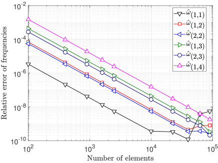
Figure 3: Vibrating square plate under zero pre-load: Relative error of the natural frequencies $\hat{\omega}_{(m,n)}=\omega_{(m,n)}\big{|}_{\boldsymbol{E}^{(0)}=\boldsymbol{0}}$ vs. mesh refinement. The analytical solution of (33) is used as reference. $m$ and $n$ are defined in Fig. 2. The boundary is simply supported.

As seen, the discretization error does not decrease beyond a certain refinement, since the condition number of the stiffness matrix becomes too large for an accurate solution of the problem. For the following simulation results a FE mesh with $80\times 80$ quadratic NURBS elements is considered to ensure convergence.
Second, the modal analysis of a square plate under nonlinear pure dilatation and uniaxial stretch is investigated. An isotropic square plate has repeated frequencies under pure dilatation. Under pure dilatation, the material response is isotropic, the frequencies are increasing monotonically and the order of modes does not change, see Fig. 4(a). Fig. 4(b) shows a comparison of the results with the analytical solution of Eq. (34). The comparison shows agreement for zero pre-stretch ($J=1$). As $J$ increases, differences show up due to the infinitesimal strain approximation used in the analytical solution. The material has an anisotropic response under uniaxial loading. The frequencies increase faster if the specimen is stretched along the zigzag direction rather than in other directions. In uniaxial stretch, the repeated frequencies become distinct and the order of modes can change during loading, e.g. $\omega_{(1,3)}$ is larger than $\omega_{(2,1)}$ in the unstretched structure, but beyond a certain stretch the frequencies reorder and $\omega_{(2,1)}$ become larger than $\omega_{(1,3)}$ (see Fig. 5a). In both cases, the frequencies increase up to a maximum, and the model becomes unstable if it is deformed further due to a loss of ellipticity of the elasticity tensor (e.g. vanishing shear modulus for pure dilatation). The strain for vanishing shear modulus ($\mu(\varepsilon_{a})=0$) can be analytically obtained as $\varepsilon_{a}=1/\beta\,\ln(\mu_{0}/\mu_{1})$. It should be mentioned that the classical formula for the stress-dependent frequencies [67] cannot capture the behavior correctly since it assume linear material behavior and thus predicts a linear frequency increase with the stretch, which is very different from the nonlinear behavior seen in Figs. 4(a) and 5.

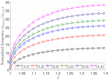
(a)

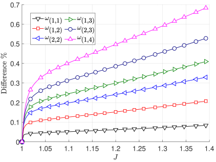
(b)

Figure 4: Vibrating square plate under pure dilatation: (4(a)) Variation of the frequencies and (4(b)) difference of the numerical results and the analytical solution of Eq. (34) in dependence of the surface stretch $J$. The plate has an edge length of 5 nm. $m$ and $n$ in $\omega_{(m,n)}$ are defined in Fig. 2. The results are normalized by $\hat{\omega}_{(1,1)}=\omega_{(1,1)}\big{|}_{J=1}$ (the first natural frequency). The boundary is simply supported.

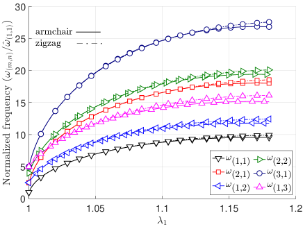
(a)

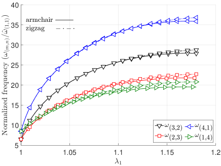
(b)

Figure 5: Vibrating square plate under uniaxial stretch: (5(a)) Frequencies 1 to 6; (5(b)) frequencies 7 to 10. $m$ and $n$ in $\omega_{(m,n)}$ are defined in Fig. 2. The edge length of the plate is 5 nm. The results are normalized by $\hat{\omega}_{(1,1)}=\omega_{(1,1)}\big{|}_{\lambda_{1}=1}$ (the first natural frequency). The plate is either stretched along the armchair or zigzag directions. The boundary is simply supported.

4.2 Vibrating circular plates

Like for the square plate, the linear modal analysis is conducted for circular plates. First, the behavior for zero pre-load is investigated. The resulting mode shapes, natural frequencies and the numbering of modes are illustrated in Figs. 6 and 7 for simply supported and clamped plates, respectively.

Figure 6: Vibrating circular plate at zero pre-load (simply supported boundary): First 8 mode shapes and natural frequencies $\hat{f}_{(m,n)}=\hat{\omega}_{(m,n)}/2\pi$ in [THz], $\hat{\omega}_{(m,n)}=\omega_{(m,n)}\big{|}_{\boldsymbol{E}^{(0)}=\boldsymbol{0}}$. $m$ and $n$ are the number of nodal diameters and circles, respectively. A nodal line is a line of material points of the plate (excluding boundaries) that do not displace during vibration.

Figure 7: Vibrating circular plate at zero pre-load (clamped boundary): First 8 mode shapes and natural frequencies $\hat{f}_{(m,n)}=\hat{\omega}_{(m,n)}/2\pi$ in [THz], $\hat{\omega}_{(m,n)}=\omega_{(m,n)}\big{|}_{\boldsymbol{E}^{(0)}=\boldsymbol{0}}$. $m$ and $n$ are the number of nodal diameters and circles, respectively. A nodal line is a line of material points of the plate (excluding boundaries) that do not displace during vibration.

A convergence study for mesh refinement is conducted and reported in Fig. 8.

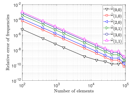
(a)

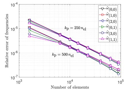
(b)

Figure 8: Vibrating circular plate under zero pre-load: Relative error of the natural frequencies for (8(a)) simply supported boundary; (8(b)) clamped boundary. The analytical solutions of (40) and (45) are used as reference. $m$ and $n$ in $\hat{\omega}_{(m,n)}=\omega_{(m,n)}\big{|}_{\boldsymbol{E}^{(0)}=\boldsymbol{0}}$ are defined in Figs. 6 and 7. The rotational dofs are fixed along the boundary by means of a penalty term using different penalty parameters $k_{\mathrm{p}}$, see Duong et al. [47] for details.

Due to ill-conditioning, the discretization error does not decrease beyond a certain refinement level. This is similar to the behavior of the square plate. For the following simulation results a FE mesh with $80\times 80$ quadratic NURBS elements is considered to ensure convergence.
Second, the vibrational behavior of a circular graphene plate under pure dilatation loading is investigated. In Fig. 9, the variation of the frequencies under pure dilatational loading is presented. As shown, the frequencies increase monotonically with $J$. The structure will become unstable if the loading is increased to far. Like for the square plate, the frequency dependency on deformation is nonlinear and cannot be captured correctly by analytical formulas based on linear elasticity.
Finally, a circular graphene plate in contact with an adhesive substrate is investigated. Locally, the substrate is modeled as a half space at each contact point and the atomic interaction is modeled via the Lennard Jones (L-J) potential. The half space potential can be written as

$$\begin{array}[]{lll}\Psi_{\text{(VdW)h}}\!\!\!&=&\!\!\!\displaystyle-\Gamma\left[\frac{3}{2}\left(\frac{h_{0}}{r}\right)^{3}-\frac{1}{2}\left(\frac{h_{0}}{r}\right)^{9}\right]~{},\end{array}$$ (21)

where $h_{0}$, $\Gamma$ and $r$ are the equilibrium distance, the interfacial adhesion energy per unit area and the normal distance of a surface point to the substrate. The derivation of the half space potential, contact force and stiffness can be found in Sauer and Li [68], Sauer and Wriggers [69] and Aitken and Huang [70]. In Fig. 10, the boundary conditions, the variation of the frequencies with increasing adhesion energy, and the first mode shape are shown. The locations with sudden frequency changes (indicated by dashed lines in Fig. 10(b)) are local instabilities where the frequency suddenly drops to zero and quickly recovers again, as the enlargement in Fig. 11(b) shows. A similar issue has been reported for loading of graphene on an adhesive substrate by Kumar et al. [53]. For these adhesion energies, the graphene surface can come very close to the substrate leading to negative eigenvalues of the contact stiffness matrix so that the eigenvalues of the total problem become very small. A large change in the frequencies and deformation can be seen at those frequencies. The softening effect of the stiffness results in the local mode shapes that are shown in Fig. 11.

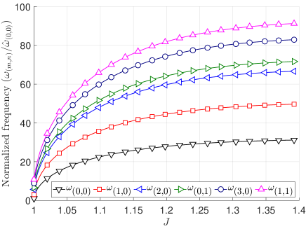
(a)

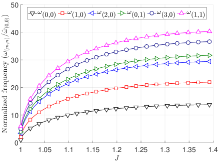
(b)

Figure 9: Vibrating circular plate under pure dilatation: Variation of the bending frequencies with the surface stretch $J$ for (9(a)) simply supported boundary; (9(b)) clamped boundary. $m$ and $n$ in $\omega_{(m,n)}$ are defined in Figs. 6 and 7. The radius of the disk is 5 nm and the results are normalized by $\hat{\omega}_{(0,0)}=\omega_{(0,0)}\big{|}_{J=1}$ (the first natural frequency).

(a)

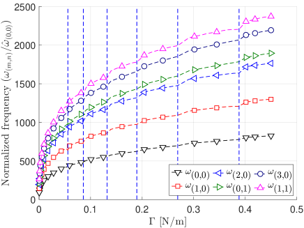
(b)

(c)

(d)

Figure 10: Vibrating circular plate on an adhesive substrate: (10(a)) Illustration of the boundary conditions; (10(b)) variation of the frequencies with the adhesion strength $\Gamma$; (10(c)) first mode shape $\omega_{(1,1)}$; (10(d)) cut of (10(c)). $m$ and $n$ in $\omega_{(m,n)}$ are defined in Fig. 6. The radii of the cavity $R_{1}$ and the fillet $R_{2}$ are 450 nm and 50 nm. The results are normalized by $\hat{\omega}_{(0,0)}=\omega_{(0,0)}\big{|}_{\Gamma=0}$ (the first natural frequency). Instability points are indicated by dashed vertical lines.

(a)

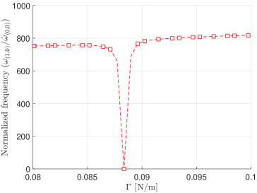
(b)

Figure 11: Vibrating circular plate on an adhesive substrate: (11(a)) Local mode near the instability point $\Gamma=0.08834~{}\mathrm{N/m}$; (11(b)) enlargement of (10(b)) for $\omega_{(1,0)}$.

4.3 Vibrating carbon nanotubes

In this section, modal analysis of CNTs is conducted to calculate the frequencies of CNTs. The model is verified in a linear regime and then the simulation is extended to the nonlinear regime. For the following simulation results a FE mesh with $160\times 160$ quadratic NURBS elements is considered to ensure convergence.
First, a linear modal analysis with free boundaries is conducted and the FE formulation is verified. The radial breathing modes can be easily computed in different numerical and experimental methods. In this mode, the radius of the CNT increases and there are no tangential displacements. The radial breathing mode should not be confused with the first torsion mode (see Fig. 12). The natural radial breathing modes of different CNTs for the proposed model are compared with other finite element, molecular dynamics, molecular mechanics, ab-initio and experimental results from the literature (Tab. 3). The quantum and experimental results of the radial breathing mode have been obtained by either using a periodic boundary condition in the axial direction or by considering very long CNTs, respectively. In Tab. 3, it has been confirmed that the radial breathing mode is converging when increasing the aspect ratio, so the proposed continuum results can be compared with atomistic and experimental results. The new results are in a good agreement with those. The frequencies from the proposed model are higher than other numerical results, but lower than (and thus closer to) experimental results. The first radial mode has a frequency that is several times larger than the first torsion mode in the current example.
Second, the influence of uniaxial stretch on the frequencies of CNTs is investigated. The CNTs are simply supported (Fig. 13) and stretched in the axial direction. The mode shapes, natural frequencies and their naming are shown in Fig. 14 for zero axial pre-tension. Figure 15 shows that the frequency of the torsion and shell modes are monotonically decreasing and increasing with stretch, respectively. In contrast, the bending beam frequencies first increase and then decrease under further stretching. The frequencies of the higher shell modes increase more than the lower shell modes, and the frequencies of the bending beam modes are changing with a similar factor for all CNTs. CNT(10,10) is stretched in the zigzag direction, which is the strongest direction, while CNT(17,0) and CNT(14,7) are stretched in other directions that are weaker than the armchair direction. So the torsion modes of CNT(17,0) and CNT(14,7) show a rapid decrease beyond $\lambda_{1}=1.142$, but the decrease is more slowly for CNT(10,10). A similar behavior should be seen for CNT(10,10), if it could be stretched further. The CNTs will become unstable if there are stretched further.

CNT($n$,$m$)	AR	PM	[71] (MD, FE)	[72] (MM)	[73] (FP)	[74] (Exp)
CNT(10,10)	5.669	5.14269	NA	5.02583	NA	NA
CNT(10,10)	10	5.13660	NA	5.01628	NA	NA
CNT(10,10)	15	5.13513	5.01783, 4.96518	NA	NA	NA
CNT(10,10)	$\infty$	5.13427	5.01783, 4.96518	NA	5.06649	5.30632
CNT(20,20)	5.669	2.57346	NA	2.51630	NA	NA
CNT(25,10)	5.669	2.85468	NA	2.79265	NA	NA
CNT(30,0)	5.669	2.47617	NA	2.42334	NA	NA
CNT(43,0)	6.052	2.07282	NA	2.02818	NA	NA

Table 3: Vibrating CNT with free boundary: The natural radial breathing frequencies [THz] according to various studies. The speed of light is taken as $2.9979\times 10^{8}$ m/s. AR = aspect ratio; PM = proposed model; MD = molecular dynamics; FE = three-dimensional finite elements; MM= molecular mechanics; FP = first principles; Exp = experimental; NA = not available.

Figure 12: Vibrating CNT with free boundary: Mode shapes: (a) Torsion mode 1 (TM1) occurring at 0.41545 THz, (b) radial breathing mode 1 (RB1) occurring at 5.13513 THz. The figures are colored by the norm of the eigenvectors.

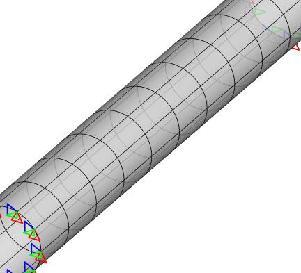
Figure 13: Vibrating CNT: Boundary conditions and finite element mesh.

Figure 14: Vibrating CNT at zero pre-tension: Mode shapes and natural frequencies $\hat{f}_{(m,n)}=\hat{\omega}_{(m,n)}/2\pi$ in [THz]: (a) Bending beam mode 1 (BB1), (b) bending beam mode 2 (BB2), (c) torsion mode 1 (TM1), (d) shell mode 1 (SH1), (e) shell mode 2 (SH2) and (f) shell mode 3 (SH3). CNT(10,10) with a length of 10 nm and simply supported boundary is used, where $m$ and $n$ in CNT$(n,m)$ are the chirality parameters. The figures are colored by the norm of the eigenvectors.

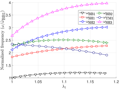
(a)

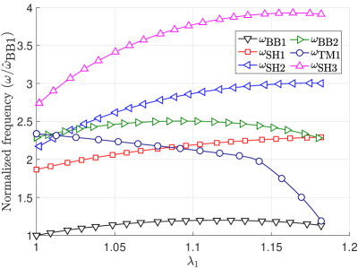
(b)

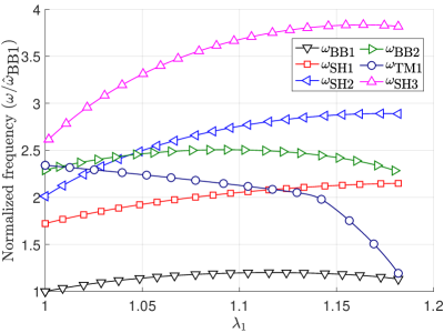
(c)

Figure 15: Vibrating CNTs under axial tension: Variation of the frequencies versus stretch $\lambda_{1}$. (15(a)) CNT(10,10), (15(b)) CNT(17,0), (15(c)) CNT(14,7). An aspect ratio of 7.3746 is used. BB, SH and TM stand for bending beam, shell and torsion modes. The boundary is simply supported.

Finally, the buckling of CNTs under compressive axial strains is investigated. CNTs buckle in bending beam or shell modes depending on their aspect ratio. The frequencies of the first and second bending beam mode become zero at $2.7\%$ and $5.4\%$ strain for CNT(7,0) with aspect ratio 15, indicating buckling (Fig. 16). Gupta et al. [75] obtain axial buckling strains of $2.2\%$ and $4.3\%$ for the same aspect ratio, which are lower than the current results. The frequencies of modes SH1, SH2, SH3, BB1 become zero at $7.14\%$, $7.56\%$, $7.8\%$ and $8.58\%$ strain for CNT(7.7) with aspect ratio 6.4. Yakobson et al. [76] and Gupta et al. [75] obtain the buckling strains $5\%$ and $9.12\%$ for the shell and bending beam modes for the same CNT.

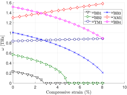
(a)

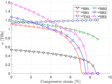
(b)

Figure 16: Vibrating CNTs under axial compression: Variation of the frequencies versus the axial strain for (16(a)) CNT(7,0) with AR=15, (16(b)) CNT(7,7) with AR=6.4. AR= aspect ratio. AM1= axial mode 1, BB4= bending beam mode 4 (see Fig. 14) for other mode shapes. The boundary is simply supported. Zero frequencies indicate buckling.

5 Conclusions

The nonlinear vibrational properties of graphene-based structures are determined with a new rotation-free shell formulation based on isogeometric finite elements. A hyperelastic material model is used to describe graphene-based structures under large deformations, accounting for nonlinear compressing, stretching and bending. The frequencies are affected strongly by those nonlinearities. Additionally, the nonlinearities of substrate interaction have a strong effect on the frequencies. A calculation based on linear elasticity can underestimate the frequencies, whereas the proposed nonlinear material model avoids this problem. It is therefore important to include the effects of pre-stretch or substrate adhesion in the modal analysis. The results of the current research can be used in the detailed design of graphene-based devices such as MEMS and NEMS. These calculations are essential to control resonance and stability. The modal analysis for square and circular plates under pure dilatation, uniaxial stretch, and substrate adhesion is conducted. The natural frequencies are verified with the analytical solutions for zero pre-load. The natural radial breathing mode of a CNT is compared with results from the literature and there is good agreement. The variation of CNT frequencies with uniaxial stretch and compression is obtained and the influence of chirality is investigated. The strains where the frequencies vanish correspond to the strain of various buckling modes. Further, the influence of chirality on the variation of the frequencies is studied. In the present study the nonlinearities due to large initial deformations, contact and constitution are considered. Another source of nonlinearity is tension modulation [77, 78]. Tension modulation describes tension that is constant in space, but varies in the time. The proposed model can be applied to many other graphene-based structures. An interesting example are the vibration of carbon nanocones [79, 80]. They can be studied in future work based the present finite element model.

Appendix A Analytical solution of natural frequencies

The natural frequencies for simply supported square and clamped/simply supported circular plates are analytically obtained for the Canham bending energy model. Here, it is shown that the shell theories based on the classical Koiter bending energy model [81, 82, 83] and Canham bending energy have the same differential equation but they have two different characteristic equations for a simply supported circular plate. This is due to the moment boundary conditions and Poisson’s ratio. The characteristic equations, which are obtained from the Koiter and Canham models, are identical for circular clamped plates. In addition, they are identical for square simply supported plates. In this section, first the mass density of graphene is calculated. Then, the characteristic equations for the different geometries and boundary conditions are derived. These solutions are used in the verification of the numerical method.

A.1 Graphene density

A hexagonal Representative Area Element (RAE) is selected to compute the mass density (Fig. 17). The area of the RAE can be computed as

$$\begin{array}[]{lll}\displaystyle A_{\mathrm{RAE}}\!\!\!&=&\!\!\!\displaystyle\frac{3\sqrt{3}}{2}\,a^{2}~{},\end{array}$$ (22)

where $a$ is the length of the carbon-carbon bond. In addition, each carbon atom is shared among three RAEs and so there are $6\times\frac{1}{3}=2$ full atoms per the RAE. Finally, the mass density in the reference configuration is computed as

$$\begin{array}[]{lll}\displaystyle\rho_{0}\!\!\!&=&\!\!\!\displaystyle\frac{2m}{A_{\mathrm{RAE}}}=0.76106\times 10^{-6}\frac{\mathrm{kg}}{\mathrm{m}^{2}}~{},\end{array}$$ (23)

where $m$ is the mass of a carbon atom and $\rho_{0}$ can be connected to the surface density in the current configuration via the area stretch $J$ as

$$\begin{array}[]{lll}\rho_{0}\!\!\!&=&\!\!\!J\,\rho~{}.\end{array}$$ (24)

Figure 17: Representative area element (RAE) for the computation of the mass density.

A.2 Equilibrium Equation

In this section, the plate equilibrium equation is derived for the Canham bending model [50, 84] in Cartesian coordinates. Then, it is transformed to operator form to be used in a cylindrical coordinate.
The Canham bending energy density per current area can be written as

$$\begin{array}[]{lll}w_{\mathrm{b}}=c\,\left(2H^{2}-\kappa\right)~{},\end{array}$$ (25)

where $H$ and $\kappa$ are the mean and Gaussian curvatures and $c$ is the bending modulus. If the strains are assumed to be infinitesimal and the shell is flat in the reference configuration, the bending deflection can be described by $z(x,y)$ and the bending strain energy density becomes

$$\begin{array}[]{lll}W_{\mathrm{b}}\!\!\!&=&\!\!\!\displaystyle c\,\left[\frac{1}{2}\left(\kappa_{xx}^{2}+\kappa_{yy}^{2}\right)+\kappa_{xy}^{2}\right]~{},\end{array}$$ (26)

where the Cartesian components of the curvature are

$$\begin{array}[]{lll}\displaystyle\kappa_{xx}\!\!\!&:=&\!\!\!z_{,xx}~{},\\[8.53581pt] \displaystyle\kappa_{yy}\!\!\!&:=&\!\!\!z_{,yy}~{},\\[8.53581pt] \displaystyle\kappa_{xy}\!\!\!&:=&\!\!\!z_{,xy}~{},\end{array}$$ (27)

where _,x and _,y denote partial differentiation w.r.t. $x$ and $y$. The Cartesian components of the bending moment are

$$\begin{array}[]{lll}M_{xx}=\displaystyle-\frac{\partial{W_{\mathrm{b}}}}{\partial{\kappa_{xx}}}=-c\,\kappa_{xx}~{},\\[8.53581pt] M_{yy}=\displaystyle-\frac{\partial{W_{\mathrm{b}}}}{\partial{\kappa_{yy}}}=-c\,\kappa_{yy}~{},\\[8.53581pt] M_{xy}=\displaystyle-\frac{\partial{W_{\mathrm{b}}}}{\partial{\kappa_{xy}}}=-c\,\kappa_{xy}~{}.\end{array}$$ (28)

The final equilibrium equation takes the well-known form [67]

$$\begin{array}[]{lll}\displaystyle\nabla^{4}(w)+\frac{\rho}{c}\,w_{,tt}\!\!\!&=&\!\!\!\displaystyle\frac{p}{c}~{}.\\ \end{array}$$ (29)

A.3 Rectangular plate: simply supported

The boundary conditions for a simply supported rectangular plate are

$$\begin{array}[]{l}\displaystyle w=0;~{}M_{xx}=-c\frac{\partial^{2}{w}}{\partial{x}^{2}}=0~{}\text{at}~{}x=\pm a~{},\\[8.53581pt] \displaystyle w=0;~{}M_{yy}=-c\frac{\partial^{2}{w}}{\partial{y}^{2}}=0~{}\text{at}~{}y=\pm b~{}.\\ \end{array}$$ (30)

where $a$ and $b$ are the half length and half width of the plate. The solution of Eq. (LABEL:e:equib_cart_w) can be decomposed into the harmonic time independent and time dependent parts as

$$\begin{array}[]{l}\displaystyle w(x,y,t)=W(x,y)\,e^{-i\hat{\omega}t}~{}.\end{array}$$ (31)

The final solution is [81, 67]

$$\begin{array}[]{l}\displaystyle w(x,y,t)=\sum\limits_{m,n=1}^{\infty}{A_{(m,n)}\,\sin\left(\frac{m\pi x}{a}\right)\,\sin\left(\frac{n\pi y}{b}\right)\,e^{-i\hat{\omega}_{(m,n)}t}}~{},\end{array}$$ (32)

where $A_{(m,n)}$ can be calculated by Fourier transformation and $\hat{\omega}_{(m,n)}$ are the natural vibration frequencies given by

$$\begin{array}[]{l}\displaystyle\hat{\omega}_{(m,n)}=\pi^{2}\,\left(\frac{m^{2}}{a^{2}}+\frac{n^{2}}{b^{2}}\right)\,\sqrt{\frac{c}{\rho}};~{}~{}\text{with}~{}~{}m,n=1,2,3,...~{}~{}.\end{array}$$ (33)

Including the effect of in-plane stresses gives

$$\begin{array}[]{lll}\displaystyle\omega_{(m,n)}^{2}\!\!\!&=&\!\!\!\displaystyle\hat{\omega}^{2}_{(m,n)}+\frac{1}{\rho}\left[N_{x}\left(\frac{\pi\,m}{a}\right)^{2}+N_{y}\left(\frac{\pi\,n}{b}\right)^{2}\right]~{},\end{array}$$ (34)

where $N_{x}$ and $N_{y}$ are the normal stress components along the $x$ and $y$ directions [81]. For the material model of Kumar and Parks [23] under pure dilatation, $N_{x}$ and $N_{y}$ can be written as

$$\begin{array}[]{lll}N_{x}=N_{y}=\displaystyle\varepsilon\,\hat{\alpha}^{2}\,\ln(J)\,e^{-(1+\hat{\alpha})\,\ln(J)}~{}.\end{array}$$ (35)

A.4 Circular plate

In this subsection, the characteristic equations of circular plates with clamped and simply supported boundary conditions are obtained.

A.4.1 Circular clamped

The boundary conditions of a clamped circular plate are

$$\begin{array}[]{l}\displaystyle w=0;~{}w_{,r}=0~{}\text{at}~{}r=a~{},\\[8.53581pt] \displaystyle w~{}\&~{}w_{,r}~{}\rightarrow~{}\text{finite}~{}\text{at}~{}r=0~{},\\ \end{array}$$ (36)

where $a$ is the radius of the plate. The solution of Eq. (LABEL:e:equib_cart_w) can be decomposed as

$$\begin{array}[]{l}\displaystyle w(r,\varphi,t)=R(r)e^{im\varphi}e^{-i\hat{\omega}t}~{}.\end{array}$$ (37)

The final solution is [81, 67]

$$\begin{array}[]{l}\displaystyle w(r,\varphi,t)=\sum\limits_{m,n=0}^{\infty}{\left[D_{(m,n)}\cos(m\varphi)+E_{(m,n)}\sin(m\varphi)\right]\,R_{(m,n)}(r)\,e^{-i\hat{\omega}_{(m,n)}t}}~{},\end{array}$$ (38)

where $R_{(m,n)}$ and $\hat{\omega}_{(m,n)}$ are

$$\begin{array}[]{l}\displaystyle R_{(m,n)}=I_{m}\left(\gamma_{(m,n)}\right)\,J_{m}\left(\frac{\gamma_{(m,n)}r}{a}\right)-J_{m}\left(\gamma_{(m,n)}\right)\,I_{m}\left(\frac{\gamma_{(m,n)}r}{a}\right)~{},\end{array}$$ (39)

$$\begin{array}[]{l}\displaystyle\hat{\omega}_{(m,n)}=\frac{\gamma_{(m,n)}^{2}}{a^{2}}\sqrt{\frac{c}{\rho}}~{},\end{array}$$ (40)

where $J_{m}$ and $I_{m}$ are the Bessel and modified Bessel functions of the first kind of order m. Furthermore, $\gamma_{(m,n)}$ are the solution of

$$\begin{array}[]{l}\displaystyle\frac{J_{m+1}(\gamma)}{J_{m}(\gamma)}+\frac{I_{m+1}(\gamma)}{I_{m}(\gamma)}=0;~{}~{}\text{with}~{}m=0,1,2,3,...~{}.\end{array}$$ (41)

$D_{(m,n)}$ and $E_{(m,n)}$ can be computed by Fourier transformation.

A.4.2 Circular simply supported

The boundary conditions of a simply supported circular plate are

$$\begin{array}[]{l}\displaystyle w=0;~{}\&~{}M_{rr}=-c\,w_{,rr}=0~{}\text{at}~{}r=a~{},\\[8.53581pt] \displaystyle w~{}\&~{}w_{,r}~{}\rightarrow~{}\text{finite}~{}\text{at}~{}r=0~{},\\ \end{array}$$ (42)

where $a$ is the radius of the plate. The final solution is [81, 67]

$$\begin{array}[]{l}\displaystyle w(r,\varphi,t)=\sum\limits_{m,n=0}^{\infty}{\left[D_{(m,n)}\,\cos(m\varphi)+E_{(m,n)}\,\sin(m\varphi)\right]\,R_{(m,n)}(r)\,e^{-i\hat{\omega}_{(m,n)}t}}~{},\end{array}$$ (43)

where $R_{(m,n)}$ and $\hat{\omega}_{(m,n)}$ are

$$\begin{array}[]{l}\displaystyle R_{(m,n)}=I_{m}\left(\gamma_{(m,n)}\right)\,J_{m}\left(\frac{\gamma_{(m,n)}r}{a}\right)-J_{m}\left(\gamma_{(m,n)}\right)\,I_{m}\left(\frac{\gamma_{(m,n)}r}{a}\right)~{},\end{array}$$ (44)

$$\begin{array}[]{l}\displaystyle\hat{\omega}_{(m,n)}=\frac{\gamma_{(m,n)}^{2}}{a^{2}}\,\sqrt{\frac{c}{\rho}}~{},\end{array}$$ (45)

where $\gamma_{(m,n)}$ are solution of

$$\begin{array}[]{l}\displaystyle\frac{J_{m+1}(\gamma)}{J_{m}(\gamma)}+\frac{I_{m+1}(\gamma)}{I_{m}(\gamma)}=2\gamma;~{}~{}\text{with}~{}~{}m=0,1,2,3,...~{}.\end{array}$$ (46)

This relation is different from the one which can be obtained for the Koiter shell theory [81].

Appendix B Stiffness and mass matrix

In this section, the finite element mass and stiffness matrices are given. They are defined based on NURBS shape functions $N_{i}$ and their parametric “,” and covariant “;” derivatives. The matrix form of NURBS shape functions and their derivatives can be written as [47]

$$\begin{array}[]{lll}\mathbf{N}\!\!\!&=&\!\!\![N_{1}\,\boldsymbol{1},N_{2}\,\boldsymbol{1},...,N_{n_{e}}\,\boldsymbol{1}]~{},\\[2.84526pt] \mathbf{N}_{,\alpha}\!\!\!&=&\!\!\![N_{1,\alpha}\,\boldsymbol{1},N_{2,\alpha}\,\boldsymbol{1},...,N_{n_{e},\alpha}\,\boldsymbol{1}]~{},\\[2.84526pt] \mathbf{N}_{,\alpha\beta}\!\!\!&=&\!\!\![N_{1,\alpha\beta}\,\boldsymbol{1},N_{2,\alpha\beta}\,\boldsymbol{1},...,N_{n_{e},\alpha\beta}\,\boldsymbol{1}]~{},\\[2.84526pt] \tilde{\mathbf{N}}_{;\alpha\beta}\!\!\!&=&\!\!\!\mathbf{N}_{,\alpha\beta}-\Gamma_{\alpha\beta}^{\gamma}\,\mathbf{N}_{,\gamma}~{},\end{array}$$ (47)

where $n_{e}$ is the number of control points per element. The mass matrix is independent of the deformation and can therefore be precomputed at the beginning of the simulation. It is

$$\begin{array}[]{lll}\mathbf{M}\!\!\!&=&\!\!\!\displaystyle\int\limits_{\mathcal{S}_{0}}{\rho_{0}\,\mathbf{N}^{T}\,\mathbf{N}\,\mathrm{d}A}~{}.\end{array}$$ (48)

The stiffness matrix can be written as

$$\begin{array}[]{lll}\mathbf{K}\!\!\!&=&\!\!\!\mathbf{k}_{\text{mat}}+\mathbf{k}_{\text{geo}}+\mathbf{k}_{\mathrm{c}}+\mathbf{k}_{\mathrm{p}}~{}.\end{array}$$ (49)

The material stiffness matrix $\mathbf{k}_{\text{mat}}$ can be written as

$$\begin{array}[]{lll}\mathbf{k}_{\text{mat}}\!\!\!&=&\!\!\!\mathbf{k}_{\tau\tau}+\mathbf{k}_{\tau M}+\mathbf{k}_{M\tau}+\mathbf{k}_{MM},\end{array}$$ (50)

with

$$\begin{array}[]{lll}\mathbf{k}_{\tau\tau}\!\!\!&:=&\!\!\!\displaystyle\int\limits_{\mathcal{S}_{0}}{{c}^{\alpha\beta\gamma\delta}\,\mathbf{N}_{,\alpha}^{\mathrm{T}}\,(\boldsymbol{a}_{\beta}\otimes\boldsymbol{a}_{\gamma})\,\mathbf{N}_{,\delta}~{}\mathrm{d}A}~{},\\ \mathbf{k}_{\tau M}\!\!\!&:=&\!\!\!\displaystyle\int\limits_{\mathcal{S}_{0}}{{d}^{\alpha\beta\gamma\delta}\,\mathbf{N}_{,\alpha}^{\mathrm{T}}\,(\boldsymbol{a}_{\beta}\otimes\boldsymbol{n})\,\tilde{\mathbf{N}}_{;\gamma\delta}~{}\mathrm{d}A}~{},\\ \mathbf{k}_{M\tau}\!\!\!&:=&\!\!\!\displaystyle\int\limits_{\mathcal{S}_{0}}{{e}^{\alpha\beta\gamma\delta}\,\tilde{\mathbf{N}}_{;\alpha\beta}^{\mathrm{T}}\,(\boldsymbol{n}\otimes\boldsymbol{a}_{\gamma})\,\mathbf{N}_{,\delta}~{}\mathrm{d}A}~{},\\ \mathbf{k}_{MM}\!\!\!&:=&\!\!\!\displaystyle\int\limits_{\mathcal{S}_{0}}{{f}^{\alpha\beta\gamma\delta}\,\tilde{\mathbf{N}}_{;\alpha\beta}^{\mathrm{T}}\,(\boldsymbol{n}\otimes\boldsymbol{n})\,\tilde{\mathbf{N}}_{;\gamma\delta}~{}\mathrm{d}A}~{}.\end{array}$$ (51)

Furthermore, the geometrical stiffness matrix $\mathbf{k}_{\text{geo}}$ is defined as

$$\begin{array}[]{lll}\mathbf{k}_{\text{geo}}\!\!\!&:=&\!\!\!\mathbf{k}_{\tau}+\mathbf{k}_{M}~{},\end{array}$$ (52)

with

$$\begin{array}[]{lll}\mathbf{k}_{\tau}\!\!\!&:=&\!\!\!\displaystyle\int\limits_{\mathcal{S}_{0}}{\mathbf{N}_{,\alpha}\,\tau^{\alpha\beta}\,\mathbf{N}_{,\beta}~{}\mathrm{d}A}~{},\end{array}$$ (53)

$$\begin{array}[]{lll}\mathbf{k}_{M}\!\!\!&:=&\!\!\!\displaystyle\mathbf{k}_{M1}+\mathbf{k}_{M2}+\mathbf{k}_{M2}^{\mathrm{T}}~{},\end{array}$$ (54)

with

$$\begin{array}[]{lll}\mathbf{k}_{M1}\!\!\!&:=&\!\!\!\displaystyle-\int\limits_{\mathcal{S}_{0}}{b_{\alpha\beta}\,M^{\alpha\beta}_{0}\,a^{\gamma\delta}\,\mathbf{N}_{,\gamma}^{\mathrm{T}}\,(\boldsymbol{n}\otimes\boldsymbol{n})\,\mathbf{N}_{,\delta}~{}\mathrm{d}A}~{},\\ \mathbf{k}_{M2}\!\!\!&:=&\!\!\!\displaystyle-\int\limits_{\mathcal{S}_{0}}{M^{\alpha\beta}_{0}\,\mathbf{N}_{,\gamma}^{\mathrm{T}}\,(\boldsymbol{n}\otimes\,a^{\gamma})\,\tilde{\mathbf{N}}_{;\alpha\,\beta}~{}\mathrm{d}A}~{}.\end{array}$$ (55)

The elasticity tensors of ${c}^{\alpha\beta\gamma\delta}$ , ${d}^{\alpha\beta\gamma\delta}$ , ${e}^{\alpha\beta\gamma\delta}$ and ${f}^{\alpha\beta\gamma\delta}$ are given in Ghaffari et al. [24] for graphene based on the definition in Sauer and Duong [46]. The contact stiffness matrix $\mathbf{k}_{\mathrm{c}}$ is given in Ghaffari et al. [24]. Clamped boundary conditions are applied with a penalty parameter and its stiffness matrix $\mathbf{k}_{\mathrm{p}}$ is given in Duong et al. [47].

References

- Akinwande et al. [2017] D. Akinwande, C. J. Brennan, J. S. Bunch, P. Egberts, J. R. Felts, H. Gao, R. Huang, J.-S. Kim, T. Li, Y. Li, K. M. Liechti, N. Lu, H. S. Park, E. J. Reed, P. Wang, B. I. Yakobson, T. Zhang, Y.-W. Zhang, Y. Zhou, Y. Zhu, A review on mechanics and mechanical properties of 2D materials-—graphene and beyond, Extreme Mech. Lett. 13 (2017) 42–77.
- Balandin [2011] A. A. Balandin, Thermal properties of graphene and nanostructured carbon materials, Nat. Mater. 10 (2011) 569–581.
- Renteria et al. [2014] J. D. Renteria, D. L. Nika, A. A. Balandin, Graphene Thermal Properties: Applications in Thermal Management and Energy Storage, Appl. Sci. 4 (2014) 525–547.
- Lemme [2010] M. Lemme, Current Status of Graphene Transistors, in: Gettering and Defect Engineering in Semiconductor Technology XIII, volume 156 of Solid State Phenomena, Trans Tech Publications, 2010, pp. 499–509.
- Schwierz [2010] F. Schwierz, Graphene transistors, Nat. Nanotechnol. 5 (2010) 487–496.
- Berashevich and Chakraborty [2010] J. Berashevich, T. Chakraborty, Graphene and graphane: New stars of nanoscale electronics, ArXiv e-prints (2010). DOI: arXiv:1003.6044.
- Pumera [2011] M. Pumera, Graphene in biosensing, Mater. Today 14 (2011) 308–315.
- Fazelzadeh and Ghavanloo [2014] S. A. Fazelzadeh, E. Ghavanloo, Nanoscale mass sensing based on vibration of single-layered graphene sheet in thermal environments, Acta Mech. Sin. 30 (2014) 84–91.
- Chen et al. [2013] C. Chen, S. Lee, V. V. Deshpande, G.-H. Lee, M. Lekas, K. Shepard, J. Hone, Graphene mechanical oscillators with tunable frequency, Nat. Nanotechnol. 8 (2013) 923–927.
- Natsuki [2015] T. Natsuki, Theoretical Analysis of Vibration Frequency of Graphene Sheets Used as Nanomechanical Mass Sensor, Electronics 4 (2015) 723–738.
- Kim et al. [2016] C.-W. Kim, M. D. Dai, K. Eom, Finite-size effect on the dynamic and sensing performances of graphene resonators: the role of edge stress, Beilstein J. Nanotechnol. 7 (2016) 685–696.
- Gupta and Batra [2010] S. S. Gupta, R. C. Batra, Elastic Properties and Frequencies of Free Vibrations of Single-Layer Graphene Sheets, J. Comput. Theor. Nanosci. 7 (2010) 2151–2164.
- Mustapha [2015] K. Mustapha, Vibration analysis of a pre-stressed graphene sheet embedded in a deformable matrix, arXiv preprint (2015). DOI: arXiv:1602.07658.
- Murmu and Pradhan [2009] T. Murmu, S. C. Pradhan, Vibration analysis of nano-single-layered graphene sheets embedded in elastic medium based on nonlocal elasticity theory, J. Appl. Phys. 105 (2009) 064319.
- Lee and Chang [2014] H.-L. Lee, W.-J. Chang, Vibration analysis of a graphene-substrate structure, Jpn. J. Appl. Phys. 53 (2014) 095102.
- Lee et al. [2014] H.-L. Lee, Y.-C. Yang, W.-J. Chang, Transverse Vibration of Circular Double-Layer Graphene Sheets Using Nonlocal Elasticity Theory, Microsc. Microanal. 20 (2014) 1772–1773.
- Sadeghi and Naghdabadi [2010] M. Sadeghi, R. Naghdabadi, Nonlinear vibrational analysis of single-layer graphene sheets, Nanotechnology 21 (2010) 105705.
- Li et al. [2015] H. Li, Y. Li, X. Wang, X. Huang, Nonlinear vibration characteristics of graphene/piezoelectric sandwich films under electric loading based on nonlocal elastic theory, J. Sound Vib. 358 (2015) 285–300.
- Favata and Podio-Guidugli [2012] A. Favata, P. Podio-Guidugli, A new CNT-oriented shell theory, Eur. J. Mech. - A/Solids 35 (2012) 75–96.
- Ansari et al. [2014] R. Ansari, H. Rouhi, S. Sahmani, Free vibration analysis of single- and double-walled carbon nanotubes based on nonlocal elastic shell models, J. Vib. Control 20 (2014) 670–678.
- Hussain et al. [2017] M. Hussain, M. N. Naeem, A. Shahzad, M. He, Vibrational behavior of single-walled carbon nanotubes based on cylindrical shell model using wave propagation approach, AIP Adv. 7 (2017) 045114.
- Li et al. [2016] P. Li, R. Hebibul, L. Zhao, Z. Li, Y. Zhao, Z. Jiang, Vibration and large deformation simulation analysis of graphene membrane for nanomechanical applications, in: 2016 IEEE 11th Annual International Conference on Nano/Micro Engineered and Molecular Systems (NEMS), 2016, pp. 209–212.
- Kumar and Parks [2014] S. Kumar, D. M. Parks, On the hyperelastic softening and elastic instabilities in graphene, Proceedings of the Royal Society of London A: Mathematical, Physical and Engineering Sciences 471 (2014).
- Ghaffari et al. [2018] R. Ghaffari, T. X. Duong, R. A. Sauer, A new shell formulation for graphene structures based on existing ab-initio data, Int. J. Solids Struct. 135 (2018) 37–60.
- Kumar et al. [2013] T. P. Kumar, S. Narendar, S. Gopalakrishnan, Thermal vibration analysis of monolayer graphene embedded in elastic medium based on nonlocal continuum mechanics, Compos. Struct. 100 (2013) 332–342.
- Wang and Hu [2015] L. Wang, H. Hu, Thermal vibration of a circular single-layered graphene sheet with simply supported or clamped boundary, J. Sound Vib. 349 (2015) 206–215.
- Mohammadi et al. [2014] M. Mohammadi, A. Farajpour, M. Goodarzi, F. Dinari, Thermo-mechanical vibration analysis of annular and circular graphene sheet embedded in an elastic medium, Lat. Am. J. SOLIDS Struct. 11 (2014) 659–682.
- Biswal and Rao [2015] T. Biswal, L. B. Rao, Thermo-Mechanical Vibration Analysis of Micro-Nano Scale Circular Plate Resting on an Elastic Medium, J. Nanosci. Nanotechnol. 1 (2015) 49–55.
- Kitipornchai et al. [2005] S. Kitipornchai, X. Q. He, K. M. Liew, Continuum model for the vibration of multilayered graphene sheets, Phys. Rev. B 72 (2005) 075443.
- Allahyari and Fadaee [2016] E. Allahyari, M. Fadaee, Analytical investigation on free vibration of circular double-layer graphene sheets including geometrical defect and surface effects, Compos. B. Eng. 85 (2016) 259–267.
- Ke et al. [2012] L.-L. Ke, Y.-S. Wang, J. Yang, S. Kitipornchai, Free vibration of size-dependent mindlin microplates based on the modified couple stress theory, J. Sound Vib. 331 (2012) 94–106.
- Chowdhury et al. [2011] R. Chowdhury, S. Adhikari, F. Scarpa, M. I. Friswell, Transverse vibration of single-layer graphene sheets, J. Phys. D: Appl. Phys. 44 (2011) 205401.
- Arash and Wang [2011] B. Arash, Q. Wang, Vibration of single- and double-layered graphene sheets, J. Nanotechnol. Eng. Med. 2 (2011) 011012.
- Strozzi et al. [2014] M. Strozzi, L. I. Manevitch, F. Pellicano, V. V. Smirnov, D. S. Shepelev, Low-frequency linear vibrations of single-walled carbon nanotubes: Analytical and numerical models, J. Sound Vib. 333 (2014) 2936–2957.
- Arghavan and Singh [2011] S. Arghavan, A. Singh, On the vibrations of single-walled carbon nanotubes, J. Sound Vib. 330 (2011) 3102–3122.
- Brenner [1990] D. W. Brenner, Empirical potential for hydrocarbons for use in simulating the chemical vapor deposition of diamond films, Phys. Rev. B 42 (1990) 9458–9471.
- Brenner et al. [2002] D. W. Brenner, O. A. Shenderova, J. A. Harrison, S. J. Stuart, B. Ni, S. B. Sinnott, A second-generation reactive empirical bond order (REBO) potential energy expression for hydrocarbons, J. Phys.: Condens. Matter 14 (2002) 783–802.
- Arroyo and Belytschko [2004] M. Arroyo, T. Belytschko, Finite crystal elasticity of carbon nanotubes based on the exponential Cauchy-Born rule, Phys. Rev. B 69 (2004) 115415.
- Cao [2014] G. Cao, Atomistic studies of mechanical properties of graphene, Polymers 6 (2014) 2404.
- Kudin et al. [2001] K. N. Kudin, G. E. Scuseria, B. I. Yakobson, BN, and C nanoshell elasticity from ab initio computations, Phys. Rev. B 64 (2001) 235406.
- Lee et al. [2008] C. Lee, X. Wei, J. W. Kysar, J. Hone, Measurement of the elastic properties and intrinsic strength of monolayer graphene, Science 321 (2008) 385–388.
- Sajadi et al. [2017] B. Sajadi, F. Alijani, D. Davidovikj, J. H. Goosen, P. G. Steeneken, F. van Keulen, Experimental characterization of graphene by electrostatic resonance frequency tuning, J. Appl. Phys. 122 (2017) 234302.
- Hughes et al. [2005] T. Hughes, J. Cottrell, Y. Bazilevs, Isogeometric analysis: CAD, finite elements, NURBS, exact geometry and mesh refinement, Comput. Methods in Appl. Mech. Eng. 194 (2005) 4135–4195.
- Sauer et al. [2014] R. A. Sauer, T. X. Duong, C. J. Corbett, A computational formulation for constrained solid and liquid membranes considering isogeometric finite elements, Comput. Methods in Appl. Mech. Eng. 271 (2014) 48–68.
- Roohbakhshan et al. [2016] F. Roohbakhshan, T. X. Duong, R. A. Sauer, A projection method to extract biological membrane models from 3D material models, J. Mech. Behav. Biomed. Mater. 58 (2016) 90–104.
- Sauer and Duong [2017] R. A. Sauer, T. X. Duong, On the theoretical foundations of thin solid and liquid shells, Math. Mech. Solids 22 (2017) 343–371.
- Duong et al. [2017] T. X. Duong, F. Roohbakhshan, R. A. Sauer, A new rotation-free isogeometric thin shell formulation and a corresponding continuity constraint for patch boundaries, Comput. Methods in Appl. Mech. Eng. 316 (2017) 43–83. Special Issue on Isogeometric Analysis: Progress and Challenges.
- Roohbakhshan and Sauer [2016] F. Roohbakhshan, R. A. Sauer, Isogeometric nonlinear shell elements for thin laminated composites based on analytical thickness integration, J. Micro. Mol. Phys. 01 (2016) 1640010.
- Roohbakhshan and Sauer [2017] F. Roohbakhshan, R. A. Sauer, Efficient isogeometric thin shell formulations for soft biological materials, Biomech. Model. Mechanobiol. 16 (2017) 1569–1597.
- Canham [1970] P. Canham, The minimum energy of bending as a possible explanation of the biconcave shape of the human red blood cell, J. Theor. Biol. 26 (1970) 61–81.
- Roldán et al. [2011] R. Roldán, A. Fasolino, K. V. Zakharchenko, M. I. Katsnelson, Suppression of anharmonicities in crystalline membranes by external strain, Phys. Rev. B 83 (2011) 174104.
- Gornyi et al. [2017] I. V. Gornyi, V. Y. Kachorovskii, A. D. Mirlin, Anomalous hooke’s law in disordered graphene, 2D Mater. 4 (2017) 011003.
- Kumar et al. [2016] S. Kumar, D. Parks, K. Kamrin, Mechanistic Origin of the Ultrastrong Adhesion between Graphene and a-: Beyond van der Waals, ACS Nano 10 (2016) 6552–6562. PMID: 27347793.
- Polizzotto [2001] C. Polizzotto, Nonlocal elasticity and related variational principles, Int. J. Solids Struct. 38 (2001) 7359–7380.
- Wang and Wang [2011] K. Wang, B. Wang, Vibration of nanoscale plates with surface energy via nonlocal elasticity, Physica E 44 (2011) 448–453.
- Pérez-Garza et al. [2014] H. H. Pérez-Garza, E. W. Kievit, G. F. Schneider, U. Staufer, Highly strained graphene samples of varying thickness and comparison of their behaviour, Nanotechnology 25 (2014) 465708.
- Tomori et al. [2011] H. Tomori, A. Kanda, H. Goto, Y. Ootuka, K. Tsukagoshi, S. Moriyama, E. Watanabe, D. Tsuya, Introducing nonuniform strain to graphene using dielectric nanopillars, Appl. Phys. Express 4 (2011) 075102.
- Kim et al. [2009] K. S. Kim, Y. Zhao, H. Jang, S. Y. Lee, J. M. Kim, K. S. Kim, J.-H. Ahn, P. Kim, J.-Y. Choi, B. H. Hong, Large-scale pattern growth of graphene films for stretchable transparent electrodes, nature 457 (2009) 706–710.
- Zheng [1994] Q.-S. Zheng, Theory of representations for tensor functions—-a unified invariant approach to constitutive equations, Appl. Mech. Rev. 47 (1994) 545–587.
- Itskov [2015] M. Itskov, Tensor Algebra and Tensor Analysis for Engineers: With Applications to Continuum Mechanics, Mathematical Engineering, Springer International Publishing, 2015.
- Kumar and Parks [2016] S. Kumar, D. M. Parks, Correction to ‘on the hyperelastic softening and elastic instabilities in graphene’, Proceedings of the Royal Society of London A: Mathematical, Physical and Engineering Sciences 472 (2016).
- Lu et al. [2009] Q. Lu, M. Arroyo, R. Huang, Elastic bending modulus of monolayer graphene, J. Phys. D: Appl. Phys. 42 (2009) 102002.
- Bonet and Wood [2008] J. Bonet, R. Wood, Nonlinear Continuum Mechanics for Finite Element Analysis, Cambridge University Press, 2008.
- Eichler. et al. [2011] A. Eichler., J. Moser., J. Chaste., M. Zdrojek, I. Wilson-Rae, A. Bachtold, Nonlinear damping in mechanical resonators made from carbon nanotubes and graphene, Nat Nano 6 (2011) 339–342.
- Moser et al. [2013] J. Moser, A. Eichler, J. Chaste, A. Bachtold, Nanomechanical resonators based on nanotubes and graphene, in: 2013 Transducers Eurosensors XXVII: The 17th International Conference on Solid-State Sensors, Actuators and Microsystems (TRANSDUCERS EUROSENSORS XXVII), 2013, pp. 657–660.
- Kerschen [2014] G. Kerschen, Modal Analysis of Nonlinear Mechanical Systems, volume 555, Springer, 2014.
- Ugural [2009] A. Ugural, Stresses in Beams, Plates, and Shells, Computational Mechanics and Applied Analysis, third ed., CRC Press, 2009.
- Sauer and Li [2007] R. A. Sauer, S. Li, A contact mechanics model for quasi-continua, Int. J. Numer. Methods Eng. 71 (2007) 931–962.
- Sauer and Wriggers [2009] R. A. Sauer, P. Wriggers, Formulation and analysis of a three-dimensional finite element implementation for adhesive contact at the nanoscale, Comput. Methods in Appl. Mech. Eng. 198 (2009) 3871–3883.
- Aitken and Huang [2010] Z. H. Aitken, R. Huang, Effects of mismatch strain and substrate surface corrugation on morphology of supported monolayer graphene, J. Appl. Phys. 107 (2010) 123531.
- Batra and Gupta [2008] R. C. Batra, S. S. Gupta, Wall thickness and radial breathing modes of single-walled carbon nanotubes, J. Appl. Mech 75 (2008) 061010–061010–6.
- Gupta et al. [2010] S. Gupta, F. Bosco, R. Batra, Wall thickness and elastic moduli of single-walled carbon nanotubes from frequencies of axial, torsional and inextensional modes of vibration, Comput. Mater. Sci. 47 (2010) 1049–1059.
- Lawler et al. [2005] H. M. Lawler, D. Areshkin, J. Mintmire, C. White, Radial-breathing mode frequencies for single-walled carbon nanotubes of arbitrary chirality: First-principles calculations, MRS Proceedings 899 (2005).
- Kuzmany et al. [1998] H. Kuzmany, B. Burger, M. Hulman, J. Kürti, A. G. Rinzler, R. E. Smalley, Spectroscopic analysis of different types of single-wall carbon nanotubes, EPL (Europhysics Letters) 44 (1998) 518.
- Gupta et al. [2016] S. S. Gupta, P. Agrawal, R. C. Batra, Buckling of single-walled carbon nanotubes using two criteria, J. Appl. Phys. 119 (2016) 245106.
- Yakobson et al. [1996] B. I. Yakobson, C. J. Brabec, J. Bernholc, Nanomechanics of carbon tubes: Instabilities beyond linear response, Phys. Rev. Lett. 76 (1996) 2511–2514.
- Avanzini et al. [2012] F. Avanzini, R. Marogna, B. Bank, Efficient synthesis of tension modulation in strings and membranes based on energy estimation, J. Acoust. Soc. Am. 131 (2012) 897–906.
- Bank [2009] B. Bank, Energy-based synthesis of tension modulation in strings, in: Proceedings of the 12th International Conference on Digital Audio Effects (DAFx-09), 2009, pp. 365–372.
- Firouz-Abadi et al. [2011] R. Firouz-Abadi, M. Fotouhi, H. Haddadpour, Free vibration analysis of nanocones using a nonlocal continuum model, Phys. Lett. A 375 (2011) 3593–3598.
- Gandomani et al. [2016] M. R. Gandomani, M. Noorian, H. Haddadpour, M. Fotouhi, Dynamic stability analysis of single walled carbon nanocone conveying fluid, Comput. Mater. Sci. 113 (2016) 123–132.
- Leissa [1969] A. Leissa, Vibration of Plates, NASA SP, Scientific and Technical Information Division, National Aeronautics and Space Administration, 1969.
- Hagedorn and DasGupta [2007] P. Hagedorn, A. DasGupta, Vibrations and Waves in Continuous Mechanical Systems, Wiley, 2007.
- Blevins [2015] R. Blevins, Formulas for Dynamics, Acoustics and Vibration, Wiley Series in Acoustics Noise and Vibration, Wiley, 2015.
- Belay et al. [2016] T. Belay, C. I. Kim, P. Schiavone, Analytical solution of lipid membrane morphology subjected to boundary forces on the edges of rectangular membranes, Continuum Mech. Thermodyn. 28 (2016) 305–315.