A Hierarchical Multivariate Spatio-Temporal Model for Large Clustered Climate data with Annual Cycles

Abstract

We present a multivariate hierarchical space-time model to describe the joint series of monthly extreme temperatures and amounts of rainfall. Data are available for 360 monitoring stations over 60 years, with missing data affecting almost all series. Model components account for spatio-temporal dependence with annual cycles, dependence on covariates and between responses. The very large amount of data is tackled modeling the spatio-temporal dependence by the nearest neighbor Gaussian process. Response multivariate dependencies are described using the linear model of coregionalization, while annual cycles are assessed by a circular representation of time. The proposed approach allows imputation of missing values and easy interpolation of climate surfaces at the national level. The motivation behind is the characterization of the so called ecoregions over the Italian territory. Ecoregions delineate broad and discrete ecologically homogeneous areas of similar potential as regards the climate, physiography, hydrography, vegetation and wildlife, and provide a geographic framework for interpreting ecological processes, disturbance regimes, vegetation patterns and dynamics. To now, the two main Italian macro-ecoregions are hierarchically arranged into 35 zones. The current climatic characterization of Italian ecoregions is based on data and bioclimatic indices for the period 1955-1985 and requires an appropriate update.

1 Introduction

Climate elements and regimes, such as temperature, precipitation and their annual cycles, primarily affect type and distribution of plants, animals, and soils as well as their combination in complex ecosystems [3, 32]. As such, the ecological classification of climate represents one of the basic step for the definition and mapping of ecoregions, i.e. of broad ecosystems occurring in discrete geographical areas [2, 30]. In keeping with these assumptions, a hierarchical classification of the ecoregions was recently performed in Italy including climate among the main diagnostic features, together with biogeography and physiography [12]. The Italian ecoregions (see figure 1) are arranged into four hierarchically nested tiers, which consist of 2 Divisions, 7 Provinces, 11 Sections, and 33 Subsections. For each of the tiers a different climatic diagnostic detail has been adopted: different macroclimatic zones and regions characterize Divisions and Provinces, whereas different bioclimatic types and ranges in observed thermo-pluviometric data characterize Section and Subsections.

1.1 Bioclimatic classification

To now, the climatic features adopted for the diagnosis and description of the Italian ecoregions mainly refer to data and bioclimatic indices that date back to the period 1955-1985. It needs to be updated in order to validate ecoregion boundaries, summarize current and past climatic conditions of the ecoregions, assess climate impacts on ecosystems at the meso-scale and formulate reliable biodiversity conservation strategies. To these aim several models and approaches have been proposed [see 25, 34] and several limitations have been pointed out such over smoothing in the interpolation of climate variables, severe loss of precision at small spatial resolution and more. As a matter of fact, temperature and precipitation data are generally heavily discretized in both space and time and require the interpolation to climate surfaces. Interpolations are usually carried out neglecting the correlation between climatic variables and provide climate surfaces that are often over-smoothed especially at the sub-continental scale. The uncertainty of estimated temperatures and precipitations considerably increases in areas characterized by large variation in elevation or with sparse weather monitoring stations. [24] clearly state that “rigorous mapping of climatic patterns outstands as one of the mayor issues concerning climatic change”. In their paper they investigate the extent of the bioclimatic approach to develop a rigorous cartographic methodology to express climatic diversity patterns. Their work is strongly affected by the quality of climate surfaces available at the chosen scale. [31] present four approaches that summarize projected climate changes across Ontario’s ecosystems at two spatial scales (ecoregions and selected natural heritage areas). The four approaches are based on interpolated climate surfaces obtained neglecting the correlation among climatic variables and without a rigorous assessment of estimates uncertainty. The majority of the above cited works define and analyze ecoregions making extensive use of the WorldClim database. The most recent release of the WorldClim database was obtained using the work of [19] who present an updated version of an older protocol due to [25]. With this new release WorldClim includes independent spatially interpolated monthly estimates of many climate variables for global land areas, at approximately 1 $km^{2}$ spatial resolution. Monthly values of temperature (minimum, maximum and average), precipitation, solar radiation, vapor pressure and wind speed are aggregated across the target temporal range 1970-2000 using data from between 9000 and 60000 weather monitoring stations. Weather station data were interpolated using thin-plate splines with covariates including elevation, distance to the coast and three satellite-derived variables: maximum and minimum land surface temperature as well as cloud cover obtained by the MODIS satellite platform. The authors propose to use a multi-step procedure, adopting the best performing model for each region and variable. Although this solution allows for an improvement in terms of goodness of fit, it does not allow for an easy evaluation of the overall uncertainty and does not avoid the risk of over-smoothing that was already observed with the previous protocol.

1.2 The available data

Precipitation and min/max temperature data were recorded monthly at 360 monitoring stations over 60 years (1951-2010). Therefore, the overall database consists of approximately 750000 records for three variables. The data were mostly obtained from National Institutions, such as ISPRA (“Progetto Annali” and SCIA), CRA/CREA, Meteomont (Guardia Forestale) and ENEA. Furthermore, data from additional stations were acquired from numerous Italian local authorities (Regions, Provinces). Almost all time series are affected by variable amounts of missing data as shown in table 1 reporting summary statistics on percentages of missing values by stations.

	Min.	1st Qu.	Median	Mean	3rd Qu.	Max.
Rain	0.00	1.88	7.64	11.50	18.47	68.33
T. max	0.00	5.42	13.47	16.50	24.31	96.25
T. min	0.00	5.45	13.47	16.52	24.17	96.25

Table 1: Summary statistics of the percentages of missing data at monitoring station.

The observed climate variables vary consistently with the 33 ecoregional subsections, as is shown in Figure 2.

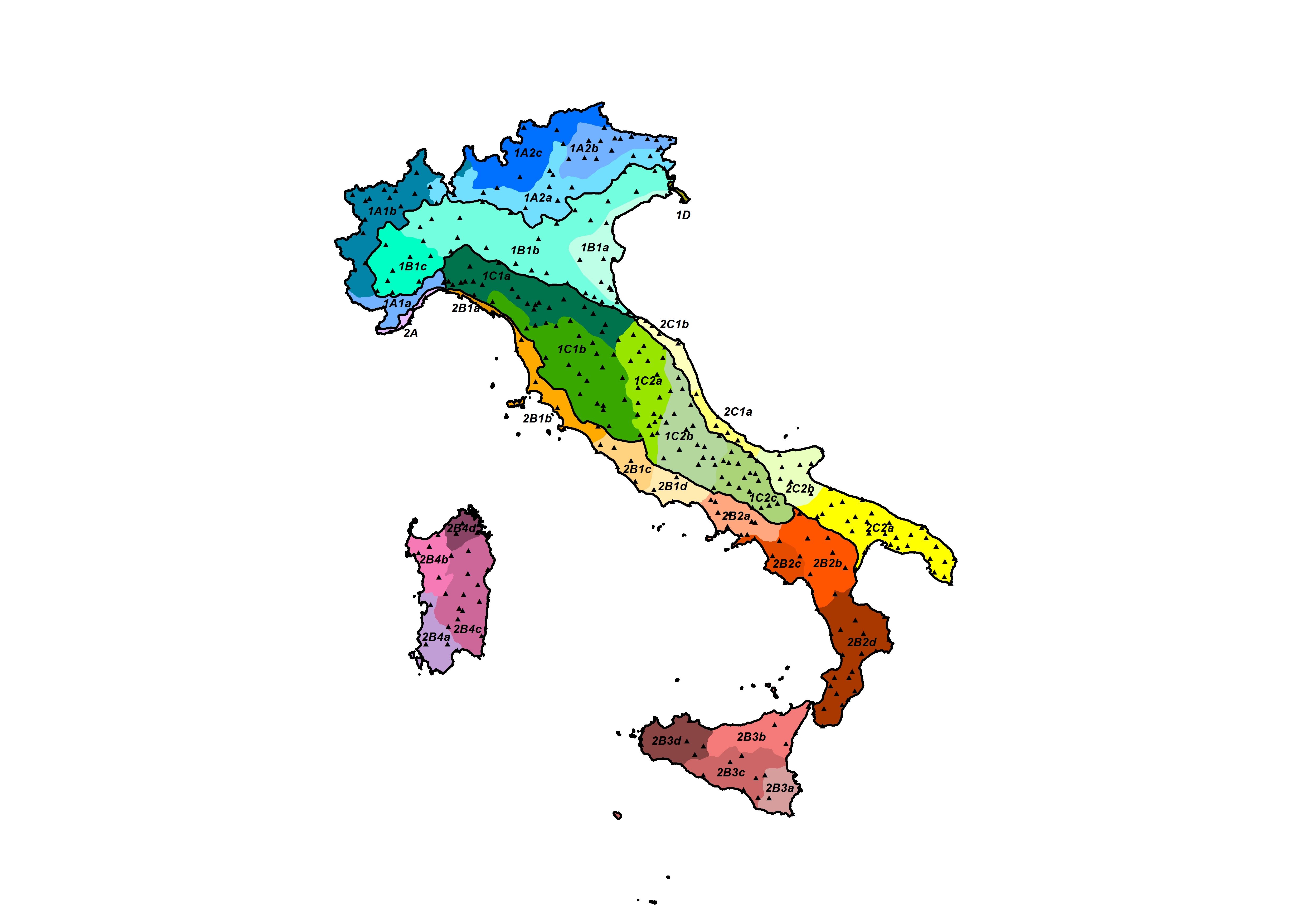
(a) $k=5$

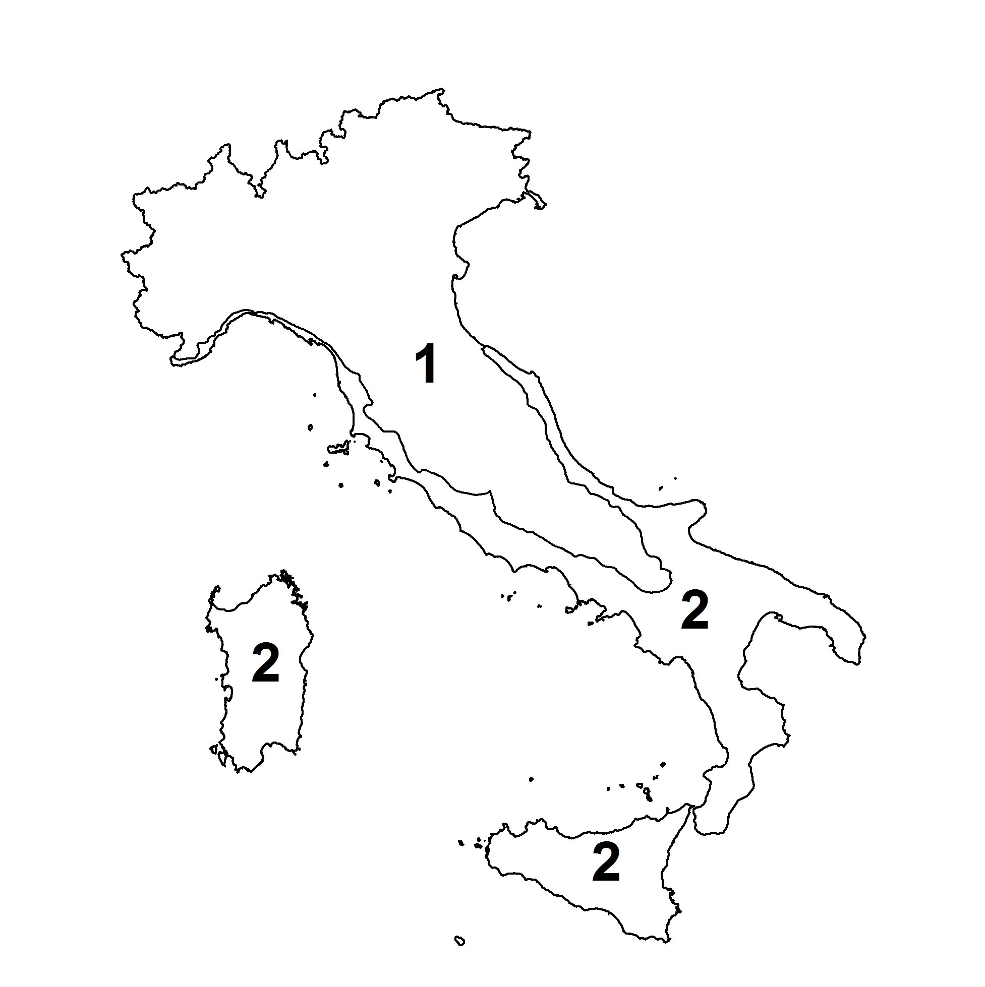
(b) $k=2$

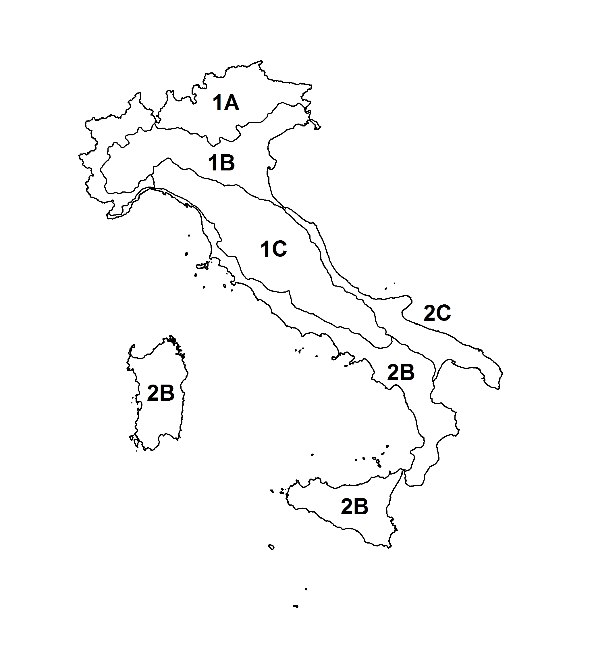
(c) $k=3$

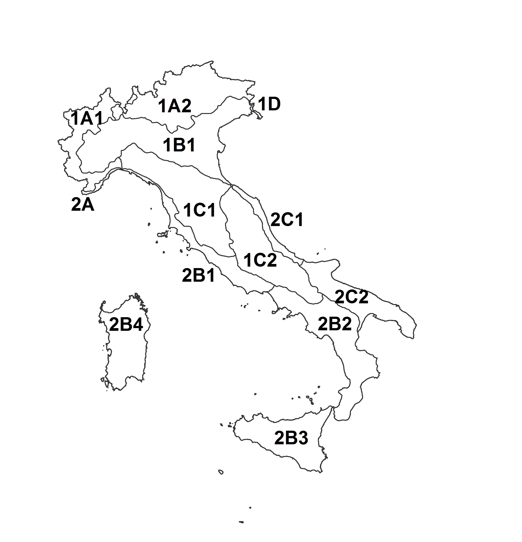
(d) $k=4$

Figure 1: Ecoregional hierarchical tier organization and climate monitoring network (a).

(a) Maximum Temperature

(b) Minimum Temperature

(c) Log-precipitation

Figure 2: Boxplots of maximum, minimum temperature and rainfall by ecoregions. Colors follow the Italian ecoregional Sections, see figure 1.

1.3 Spatio-temporal interpolation of large datasets

Bioclimatic classification requires an effective interpolation approach accounting for the correlation among climate variables and such that uncertainty evaluation is rigorously obtained. A very large amount of literature on the interpolationj of massive spatial and spatio-temporal data is now available, with some review papers [26, 28] and books [4, 21, 13] to which the interested reader is referred for details. In what follows, we restrict our interest to inferences that can be carried on at arbitrary spatial and temporal resolutions, possibly finer than those of the observed data, and to approaches that allow for a rigorous evaluation of the overall uncertainty and that are computationally feasible. The common choice would be to construct a stochastic process model to capture dependence using a spatio-temporal covariance function [21, and references therein]. While the richness and flexibility of spatio-temporal process models are indisputable, their computational feasibility and implementation pose major challenges for large datasets. Model-based inference almost always involves the calculation of inverses of large matrices, say $N\times N$, where $N$ is the number of spatio-temporal points considered. Unless the matrix is sparse or has a specific structure that eases the computation, $\mathcal{O}(N^{3})$ floating points operations would be required for any matrix inversion. Approaches for modeling large covariance matrices in purely spatial settings include low rank and covariance tapering models [21, 4, 13, and references therein] and multivariate tapering proposed in Bevilacqua et al. [7], approximations using Gaussian Markov Random Fields (GMRF), the Laplace transform and Stochastic Partial differential Equations [35, 36, 29, 9, 8], products of lower dimensional conditional densities [see 15, 16, and references therein] and composite likelihoods [17] with the recent multivariate extension proposed in Bevilacqua et al. [6]. A large number of extensions to spatio-temporal settings have been proposed, including [14], [20] and [27] who introduce dynamic spatio-temporal low-rank spatial processes, while [39] choose a GMRF approach. All the previous works use dynamic models defined for fixed temporal lags and are not easily extended to continuous spatio-temporal domains. Continuous spatio-temporal process modeling of large data has received relatively less attention. Composite likelihoods are proposed in [1] and [5] for parameter estimation in a continuous space-time setup. Both papers focus upon constructing computationally feasible likelihood approximations and inference is restricted to parameter estimation only. Uncertainty estimates are mostly based on asymptotic results which are often inappropriate for irregularly observed data. Moreover, in both cases predictions at arbitrary locations and time points are obtained imputing estimates into an interpolator derived with a different process model. Furthermore, computations are expensive for large $N$ and may not be accurate in reflecting the predictive uncertainty. Finally, an interesting proposal was recently provided by [15] with the definition of the Nearest Neighbor Gaussian Process (NNGP) approximation for large continuous spatial datasets, extended to the spatio-temporal framework in [16].

In this work we are going to apply, introducing several novelties, the approach proposed by [16] to a multivariate spatio-temporal setting, using a generalised NNGP approximation on a multi-response problem. To this aim, we combine the NNGP with the linear model of coregionalization [22] and with a circular representation of time [see for instance 37] to include annual cycles. We obtain a computationally feasible tool that allows for multivariate interpolation with large continuous space-time data, providing an accurate evaluation of the associated uncertainties. The proposed approach is applied to the characterization of Italian ecoregions in terms of temperature and precipitation, providing successful answers to the problems mentioned above: we estimate a joint model that accounts for climate variables correlation and obtain rigorous assessment of all estimates and predictions uncertainty. We deal with a huge amount of data and avoid over-smoothing. Further, we introduce annual cycles using a novel and flexible tool, we discuss the “best” ecoregions hierarchical classification tier in terms of temperature and precipitation characterization and, eventually, we get a direct imputation of missing data.

While in section 1.2 we gave a full description of the available data and of the four ecoregion hierarchical classification tiers, the rest of the paper is organized as follows. Section 2 is dedicated to the definition of the multivariate coregionalization model for the Italian data, while section 3 contains the NNGP definition and some details of the implementation of estimates and predictions. Results are reported and commented in section 4, while section 5 contains some final remarks and addresses for future developments.

2 The Model

Let $\mbox{\boldmath$s$}\in\mathcal{S}\subset\mathbb{R}^{d}$, with $d=2$, and $t\in\mathcal{T}\subset\mathbb{R}$ be spatial and temporal coordinates respectively, and let $Y^{*}_{1}(\mbox{\boldmath$s$},t)$, $Y^{*}_{2}(\mbox{\boldmath$s$},t)$ and $Y^{*}_{3}(\mbox{\boldmath$s$},t)$ represent the precipitation level, minimum and maximum temperatures observed at $(\mbox{\boldmath$s$},t)$. Then these variables have the following constraints: $Y^{*}_{1}(\mbox{\boldmath$s$},t)\geq 0$ and $Y^{*}_{3}(\mbox{\boldmath$s$},t)\geq Y^{*}_{2}(\mbox{\boldmath$s$},t)$. To simplify modeling and computations, we prefer to work with latent variables defined over the entire real line $\mathbb{R}$, embedding the above constraints in the variable definitions. Latent variables $Y_{1}(\mbox{\boldmath$s$},t)$, $Y_{2}(\mbox{\boldmath$s$},t)$ and $Y_{3}(\mbox{\boldmath$s$},t)$ are defined as follows:

$$\begin{cases}Y_{1}(\mbox{\boldmath$s$},t)=Y^{*}_{1}(\mbox{\boldmath$s$},t)&\mbox{ if }Y^{*}_{1}(\mbox{\boldmath$s$},t)>0,\\ Y_{1}(\mbox{\boldmath$s$},t)\leq 0&\mbox{ if }Y^{*}_{1}(\mbox{\boldmath$s$},t)=0,\end{cases}$$ (1)

$$Y_{2}(\mbox{\boldmath$s$},t)=Y^{*}_{2}(\mbox{\boldmath$s$},t),$$

$$\begin{cases}Y_{3}(\mbox{\boldmath$s$},t)=Y^{*}_{3}(\mbox{\boldmath$s$},t)-Y^{*}_{2}(\mbox{\boldmath$s$},t)&\mbox{ if }Y^{*}_{3}(\mbox{\boldmath$s$},t)-Y^{*}_{2}(\mbox{\boldmath$s$},t)>0,\\ Y_{3}(\mbox{\boldmath$s$},t)\leq 0&\mbox{ if }Y^{*}_{3}(\mbox{\boldmath$s$},t)-Y^{*}_{2}(\mbox{\boldmath$s$},t)=0.\end{cases}$$ (2)

Each latent response $Y_{i}$, $i=1,2,3$ is described by a combination of fixed and random terms:

$$Y_{i}(\mbox{\boldmath$s$},t)=\mathbf{X}(\mbox{\boldmath$s$})\boldsymbol{\beta}_{z_{k}}(\mbox{\boldmath$s$})+\omega_{i}(\mbox{\boldmath$s$},t)+\lambda_{i}(\mbox{\boldmath$s$},t)+\epsilon_{i}(\mbox{\boldmath$s$},t)$$ (3)

with $\epsilon_{i}(\mbox{\boldmath$s$},t)\stackrel{{\scriptstyle iid}}{{\sim}}N(0,\sigma_{\epsilon,i}^{2})$. Here $\mathbf{X}(\mbox{\boldmath$s$})=(1,X(\mbox{\boldmath$s$}))$ and $X(\mbox{\boldmath$s$})$ is the elevation of site $s$. The integer valued indicator $z_{k}(\mbox{\boldmath$s$})\subset{\mathbb{Z}^{+}}$ is the ecoregion label for the $k^{th}$ ecoregion tier: with $k=1$ we have one ecoregion covering the entire country, while $k=5$ returns the finer classification with 35 ecoregions. In general $z_{1}(\mbox{\boldmath$s$})=1$, $z_{2}(\mbox{\boldmath$s$})\in\{1,2\}$, $z_{3}(\mbox{\boldmath$s$})\in\{1,2,\dots 7\}$, $z_{4}(\mbox{\boldmath$s$})\in\{1,2,\dots 13\}$ and $z_{5}(\mbox{\boldmath$s$})\in\{1,2,\dots 35\}$. Then $\boldsymbol{\beta}_{z_{k}}=(\beta_{0,z_{k}},\beta_{1,z_{k}})^{\prime}$ are regression coefficients, varying with the ecoregion. The term $\lambda_{i}(\mbox{\boldmath$s$},t)$ describes the monthly effect of the annual cyclical behavior. More precisely, we represent time on a circular scale with 1 year period. We assume that $h^{*}_{t}=h_{t}\mod L$ is a circular variable with period $L=1$years, where $h_{t}=|t_{l}-t_{d}|$ is the temporal lag. This choice implies that e.g.: if $h_{t}=1$years, then $h_{t}^{*}=h_{t}\mod 1$year $=0$; if $h_{t}=1.1$years, then $h^{*}_{t}=0.1$ and so on. Then assuming $\lambda_{i}(\mbox{\boldmath$s$},t)\perp\lambda_{i}(\mbox{\boldmath$s$}^{\prime},t)$ for all $t$’s and $i$’s, we describe the monthly effect of the annual cyclical behavior of each response by:

$$\lambda_{i}(\mbox{\boldmath$s$},t)\sim N\left(0,\sigma^{2}_{cy,i}\exp(-\phi_{cy,i}h^{*}_{t})\right),\;\;i=1,2,3$$ (4)

where $\sigma^{2}_{cy,i},\phi_{cy,i}>0$ holds for both annual cyclical parameters.

Finally, the term $\omega_{i}(\mbox{\boldmath$s$},t)$ in (3) is defined as a multivariate spatio-temporal Gaussian process (GP) with dependent components. First we consider the multivariate GP $\mathbf{w}(\mbox{\boldmath$s$},t)=(w_{1}(\mbox{\boldmath$s$},t),w_{2}(\mbox{\boldmath$s$},t),w_{3}(\mbox{\boldmath$s$},t))^{\prime}$, where $w_{i}(\mbox{\boldmath$s$},t)\perp w_{j}(\mbox{\boldmath$s$},t)$, for all $(\mbox{\boldmath$s$},t)$’s and $w_{i}\sim GP(\mathbf{0},C(h_{\mbox{\boldmath$s$}},h_{t};\boldsymbol{\theta}_{i}))$ where $C(h_{\mbox{\boldmath$s$}},h_{t};\boldsymbol{\theta}_{i})$ is a spatio-temporal correlation function and where $h_{\mbox{\boldmath$s$}}=||\mbox{\boldmath$s$}_{l}-\mbox{\boldmath$s$}_{q}||$ and $h_{t}$ are the spatial and temporal distances with $(h_{\mbox{\boldmath$s$}},h_{t})\in\mathbb{R}^{2}\times\mathbb{R}$. We choose the general non-separable space-time correlation structure proposed by [23], defining $C(\cdot,\cdot;\cdot)$ as in his equation (14), i.e.:

$$C(h_{\mbox{\boldmath$s$}},h_{t};\boldsymbol{\theta}_{i})=\frac{1}{(\phi_{ti,i}|h_{t}|^{2\alpha_{i}}+1)^{\tau}}\exp\left(-\frac{\phi_{sp,i}\|h_{\mbox{\boldmath$s$}}\|^{2\gamma_{i}}}{(\phi_{ti,i}|h_{t}|^{2\alpha_{i}}+1)^{\eta_{i}\gamma_{i}}}\right).$$ (5)

Non-negative scaling parameters $\phi_{ti,i}$ and $\phi_{sp,i}$ are associated to time and space respectively, the smoothness parameters $\alpha_{i}$ and $\gamma_{i}$ take values in $(0,1]$, the space-time interaction parameter $\eta_{i}$ ranges in $[0,1]$ and $\tau\geq d/2$. Following both [23] and [15], we set $\tau=1$, $\alpha=1$ and $\gamma=0.5$. Attractively, as $\eta_{i}$ decreases towards zero, we achieve separability in space and time. Using the independent components of $\mathbf{w}$ , we can now define $\boldsymbol{\omega}(\mbox{\boldmath$s$},t)=(\omega_{1}(\mbox{\boldmath$s$},t),\omega_{2}(\mbox{\boldmath$s$},t),\omega_{3}(\mbox{\boldmath$s$},t))^{\prime}$ as follows:

$$\boldsymbol{\omega}(\mbox{\boldmath$s$},t)=\mathbf{A}\mathbf{w}(\mbox{\boldmath$s$},t)\;$$ (6)

where $\mathbf{A}\mathbf{A}^{\prime}=\mbox{Cov}\left(\omega_{1},\omega_{2},\omega_{3}\right)=\mbox{\boldmath$\Sigma$}$. Now, letting $\mathbf{T}_{i}=\mbox{$\mathbf{a}$ }_{i}\mbox{$\mathbf{a}$ }_{i}^{\prime}$, where $\mathbf{a}_{i}$ is the $i^{th}$ column of $\mathbf{A}$ , the covariance matrix for the process $\boldsymbol{\omega}$ at different times and locations is given by:

$$\mbox{\boldmath$\Sigma$}_{l,q}=\mbox{Cov}(\boldsymbol{\omega}(\mbox{\boldmath$s$}_{l},t_{l}),\boldsymbol{\omega}(\mbox{\boldmath$s$}_{q},t_{q}))=\sum_{i=1}^{3}\mathbf{T}_{i}C\left((||\mbox{\boldmath$s$}_{l}-\mbox{\boldmath$s$}_{q}||,|t_{l}-t_{q}|);\boldsymbol{\theta}_{i}\right).$$ (7)

Remark that the choice of $\mathbf{A}$ in equation (6) is not unique and has specific consequences on the process structure [22], hence a careful choice is required. A popular choice is the Cholesky decomposition of the symmetric matrix $\Sigma$ that produces a lower diagonal matrix. This decomposition induces an artificial ordering of the response variables in this setting, given that the correlation structure of $\omega_{1}$ depends only on $C(\cdot,\cdot;\boldsymbol{\theta}_{1})$, the one of $\omega_{2}$ depends on $C(\cdot,\cdot;\boldsymbol{\theta}_{1})$ and $C(\cdot,\cdot;\boldsymbol{\theta}_{2})$, while the correlation of $\omega_{3}$ depends on $C(\cdot,\cdot;\boldsymbol{\theta}_{1})$, $C(\cdot,\cdot;\boldsymbol{\theta}_{2})$ and $C(\cdot,\cdot;\boldsymbol{\theta}_{3})$. To avoid this artificial ordering, we propose to decompose by $\Sigma$ by a different approach: let $\boldsymbol{\Gamma}=diag(\gamma_{1},\gamma_{2},\gamma_{3})$ be the diagonal matrix of the square rooted eigenvalues of $\Sigma$ and $\boldsymbol{\Psi}$ be the orthogonal matrix of its eigenvectors, such that $\boldsymbol{\Psi}^{\prime}\boldsymbol{\Psi}=\mathbf{I}$, we then let $\mathbf{A}=\boldsymbol{\Psi}\boldsymbol{\Gamma}\boldsymbol{\Psi}^{\prime}$. Such matrix $\mathbf{A}$ is symmetric by construction and its elements do not depend on the ordering of the eigenvalues. Assume that $\mathbf{D}$ is a $3\times 3$ matrix that changes the ordering of the elements of $\boldsymbol{\omega}(\mathbf{s},t)$. The covariance matrix of $\mathbf{D}\boldsymbol{\omega}$ is then $\mathbf{D}\boldsymbol{\Sigma}\mathbf{D}^{\prime}$ with eigenvectors as the columns of matrix $\mathbf{D}\boldsymbol{\Psi}$. Now let $\mathbf{D}\boldsymbol{\Sigma}\mathbf{D}^{\prime}=\mathbf{A}_{*}\mathbf{A}_{*}^{\prime}$, then $\mathbf{A}_{*}=\mathbf{D}\boldsymbol{\Psi}\boldsymbol{\Gamma}\boldsymbol{\Psi}^{\prime}\mathbf{D}^{\prime}=\mathbf{D}\mathbf{A}\mathbf{D}^{\prime}$, proving that $\mathbf{A}_{*}$ has the same values of $\mathbf{A}$ but arranged accordingly to the reordering matrix $\mathbf{D}$.

3 Implementation

The huge dimension of the data, i.e. 360 spatial locations observed at 720 times, does not allow the implementation of a full multivariate Gaussian process. This issue, generally referred to as “Big $n$ problem” [26], arises from the need to compute the covariance matrix of the entire multivariate process, that in our case has dimension $3*720*360=777600$. Such a big matrix has to be stored and inverted to compute the model likelihood, with a computational cost of the order of $O(777600^{3})$. This is not feasible even for very large computers or computer clusters. For this reasons, an approximated approach has to be adopted. Several approaches to obtain computationally feasible approximations of Gaussian processes have been proposed in the literature [for example see 26, and references therein]. In this work we adopt an efficient and accurate approximation of a Gaussian process recently proposed by Datta et al. [15], namely the Nearest Neighbors Gaussian Process (NNGP).

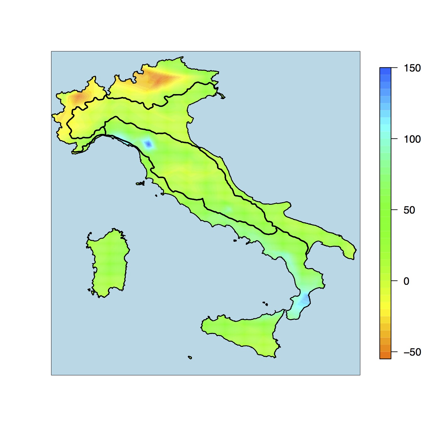
(a) Rainfall January

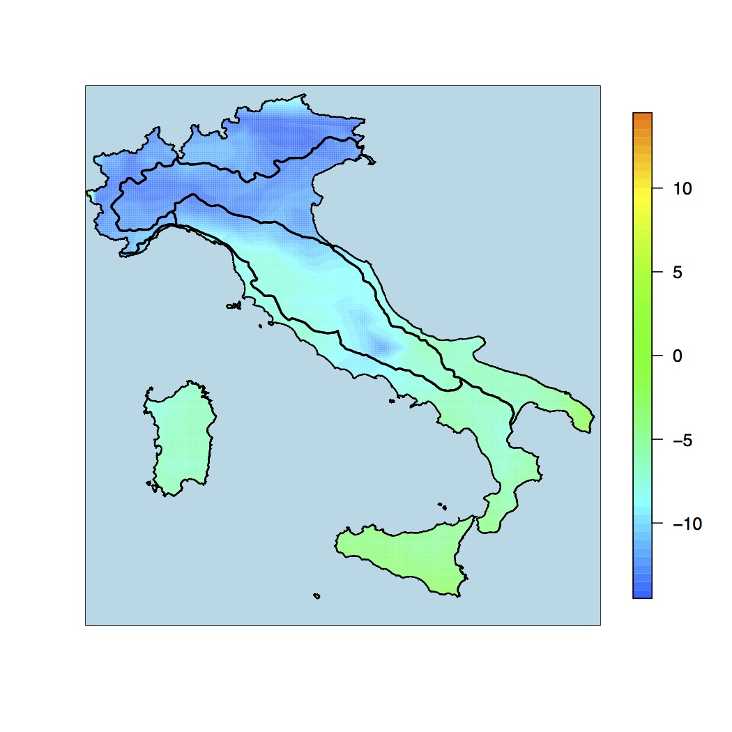
(b) Temperature min. January

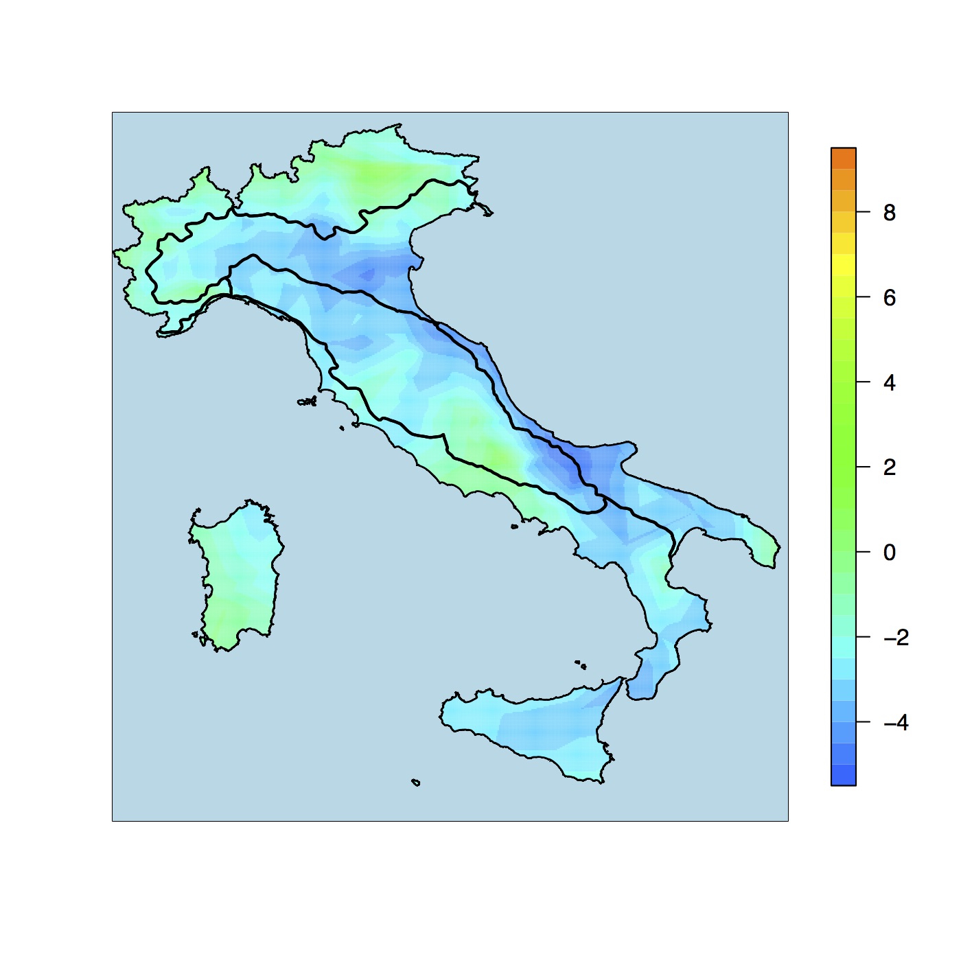
(c) $\Delta$ Temperature January

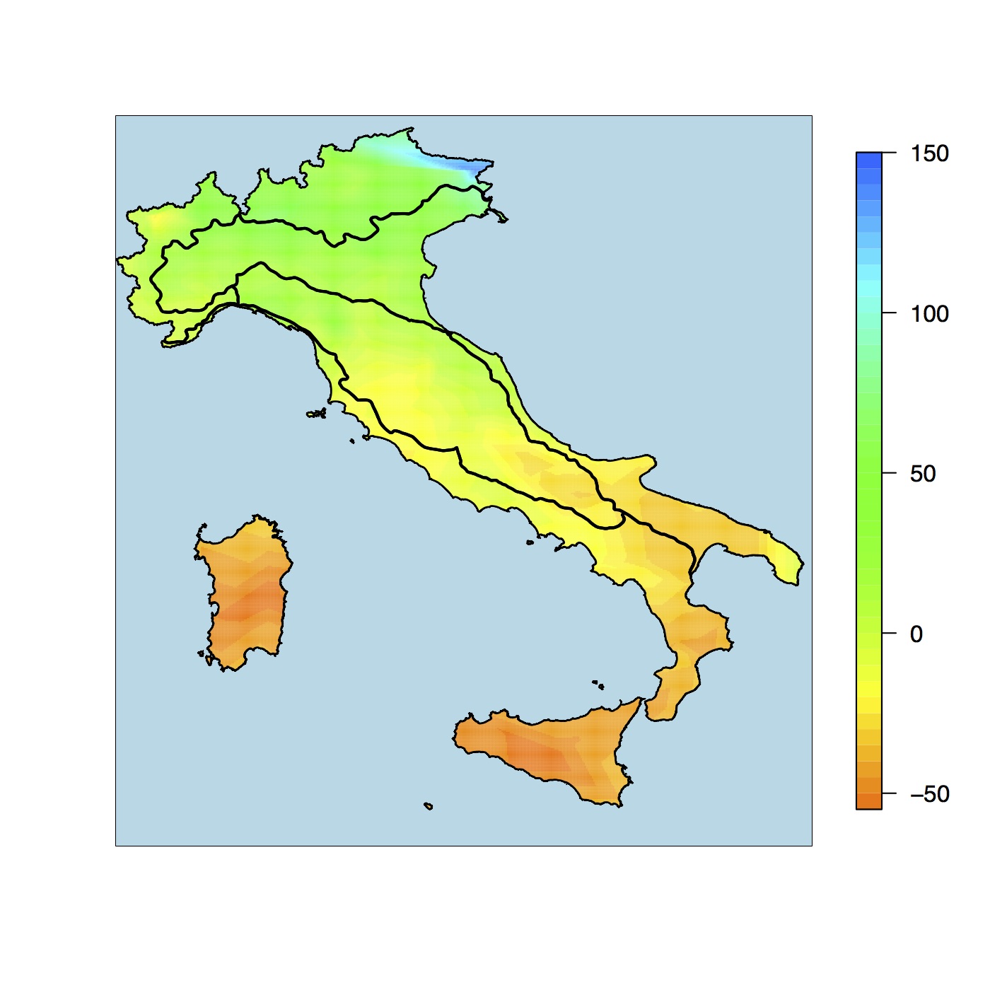
(d) Rainfall August

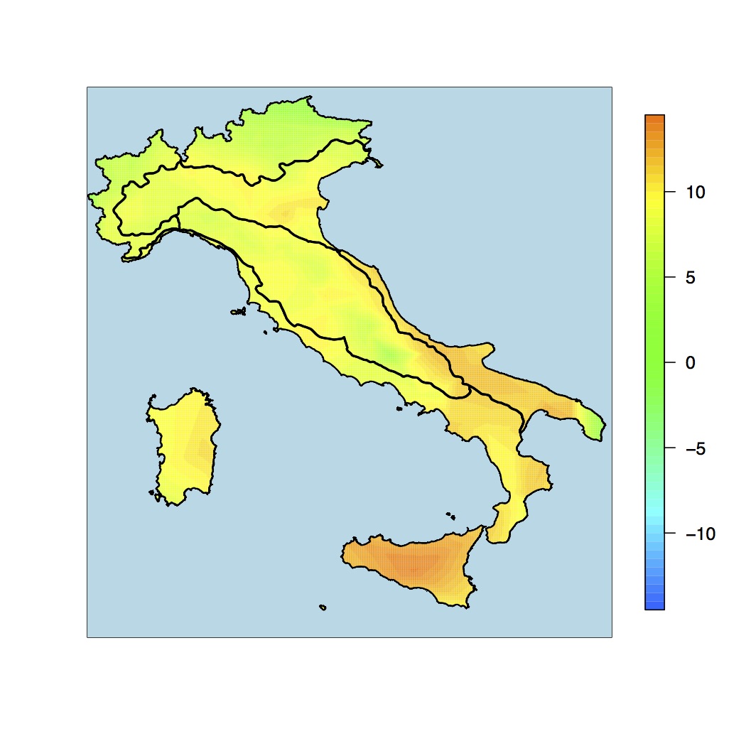
(e) Temperature min. August

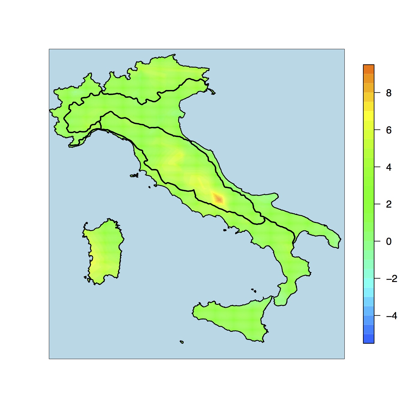
(f) $\Delta$ Temperature August

Figure 4: Maps of the monthly effects of January (a,b,c) and August (d,e,f) on the annual cycles of the three components of the process.

To address some issues related to the numerical stability of the estimation algorithm, we propose to rescale and standardize the response 6.o,6ovariables. Only in the case of the monthly rain amount, in order to preserve the information about the zeroes, we simply rescale the variable by its standard deviation. Hence, in what follows, $Y_{1}$ is rescaled while $Y_{2}$ and $Y_{3}$ are both standardized. Results are presented according to the model (transformed) scale (except for the RMSE and figure 4).

3.1 NNGP

Letting $N$ be the number of observations in space and time, we denote their locations by $(\mbox{\boldmath$s$}_{n},t_{n})$, $n=1,\dots,N$ and we let $\boldsymbol{\omega}_{n}=(\omega_{1}(\mbox{\boldmath$s$}_{n},t_{n}),\omega_{2}(\mbox{\boldmath$s$}_{n},t_{n}),\omega_{3}(\mbox{\boldmath$s$}_{n},t_{n}))^{\prime}$ with $\boldsymbol{\omega}=(\boldsymbol{\omega}_{1},\dots,\boldsymbol{\omega}_{N})^{\prime}$. If $f(\cdot)$ is a generic density function, then the joint distribution of the whole set of observations is given by

$$f(\boldsymbol{\omega})=\prod_{n=1}^{N}f(\boldsymbol{\omega}_{n}|\boldsymbol{\omega}_{n-1},\dots,\boldsymbol{\omega}_{1})$$ (8)

with $\boldsymbol{\omega}_{0}=\emptyset$. In (8) $f(\boldsymbol{\omega})$ and $f(\boldsymbol{\omega}_{n}|\boldsymbol{\omega}_{n-1},\dots,\boldsymbol{\omega}_{1})$ are Gaussian densities of size $3\cdot N$ and $3$, respectively. Notice that, though there is no univocal definition of a space-time ordering of observed locations, (8) is a valid representation of the joint density for any given ordering.

Let $\boldsymbol{\Omega}_{n}=(\boldsymbol{\omega}_{n-1},\dots,\boldsymbol{\omega}_{1})^{\prime}$ be the conditional set of $\boldsymbol{\omega}_{n}$ in (8) and let $\boldsymbol{\Omega}_{n}(m)\subseteq\boldsymbol{\Omega}_{n}$ be a set that contains at most $m$ elements of $\boldsymbol{\Omega}_{n}$. With the NNGP the joint distribution of the whole set of observations in (8) is by

$$\prod_{n=1}^{N}f(\boldsymbol{\omega}_{n}|\boldsymbol{\Omega}_{n}(m)).<$$ (9)

Indeed the quality of the approximation increases with $m$ and, as shown by [15], and the best results are achieved if we chose the $m$ elements of $\boldsymbol{\Omega}_{n}$ that have the higher correlation with $\boldsymbol{\omega}_{n}$.

To implement the NNGP three decisions have to be made:

• how to order the observations;

• how to choose the the value of $m$;

• how to choose the elements of $\boldsymbol{\Omega}_{n}(m)\subseteq\boldsymbol{\Omega}_{n}$.

The ordering

A natural ordering is immediately available for the time dimension, but there is not a unique way to order observations in space at a given time. The way we order spatial locations has a strong influence on the definition of how candidate locations enter $\boldsymbol{\Omega}_{n}(m)$. Here we follow Datta et al. [15] and order locations first according to one of the two coordinates and then according to the other. This ensures that $\boldsymbol{\Omega}_{n}$ includes observations spatially and temporally close to $\boldsymbol{\omega}_{n}$.

The value of $m$

Compared to the size of the problem, the number of neighbors $m$ should be small in order to obtain a computational gain. Datta et al. [16] showed that, assuming that the elements of $\boldsymbol{\Omega}_{n}(m)$ are “close enough” (correlated or geographically close) to $\boldsymbol{\omega}_{n}$, $m\in\{10,\dots,20\}$ produces an approximation almost indistinguishable from the original process.

The elements in $\boldsymbol{\Omega}_{n}(m)$

Again, following Datta et al. [16], the best choice for $\boldsymbol{\Omega}_{n}(m)$ is to take the $m$ elements that have higher correlation with $\boldsymbol{\omega}_{n}$. In a purely univariate temporal or spatial setting, assuming that the correlation decreases with the distance, the optimal choice for the elements $\boldsymbol{\Omega}_{n}(m)$ would consider observations spatially/temporally closer to $\boldsymbol{\omega}_{n}$. In a spatio-temporal setting with non-separable correlation function, there is not a one to one relation between distances and correlation, since a spatio-temporal distance is not uniquely defined. In an univariate spatio-temporal setting, Datta et al. [16] propose an adaptive approach in which $\boldsymbol{\Omega}_{n}(m)$ is defined at each MCMC iteration as the set that has the higher correlation with $\boldsymbol{\omega}_{n}$.

Basing the choice of $\boldsymbol{\Omega}_{n}(m)$ on correlations would imply to consider all possible sets of $m$ neighbors at each point for each MCMC iteration. In this work we prefer not to follow this approach, mostly for computational reasons as, unlike in Datta et al. [16], here we deal with a very large multivariate spatio-temporal data base. Hence we propose to define a spatio-temporal distance as shown in expression (10) and to include in $\boldsymbol{\Omega}_{n}(m)$ the locations with smaller distances from $\boldsymbol{\omega}_{n}$. Obviously, the spatial and temporal dimensions have different scales, so we adjust the spatio-temporal distance euristically as follows:

$$\sqrt{\left(h_{s}\frac{2}{30}\right)^{2}+h_{t}^{2}},$$ (10)

assuming that one year has the same weigh as $150$Km’s. Our choice is justified by the following considerations: in each neighborhood we want to include information on the spatial dependence, the time dependence and the cross-correlation structure, furthermore we need information on the annual cyclical component. Equation (10) ensures that the generic point $(\mbox{\boldmath$s$}_{n},t_{n})$ has approximately $m$ neighbors, $\sqrt{m}$ of which are observed at the same time and at different locations, $\sqrt{m}$ share the same spatial location and are observed at different times and the remaining are observed at different times and locations. Furthermore, in order to learn about the annual cyclical component, we may have to modify the points at the boundaries of $\boldsymbol{\Omega}_{n}(m)$. This is done in such a way that, for example, the neighborhood of location $s$-January 2000 includes location $s$-January 1999 and $s$-February 1999.

3.2 Implementation details

In our setting $E(\boldsymbol{\omega})=\mathbf{0}_{N}$, then using standard results from the multivariate normal theory, we can write

$$f(\boldsymbol{\omega}_{n}|\boldsymbol{\Omega}_{n}(m))=\phi_{3}(\boldsymbol{\omega}_{n}|\mathbf{B}_{n}\boldsymbol{\Omega}_{n}(m),\mathbf{F}_{n})$$ (11)

where $\phi_{3}(\boldsymbol{\omega}_{n}|\mathbf{B}_{n}\boldsymbol{\Omega}_{n}(m),\mathbf{F}_{n})$ is the $3-$variate normal distribution with mean $\mathbf{B}_{n}\boldsymbol{\Omega}_{n}(m)$ and covariance matrix $\mathbf{F}_{n}$. Parameters $\mathbf{B}_{n}$ and $\mathbf{F}_{n}$ depend on the Gneiting correlation function parameters, on $\boldsymbol{\Sigma}$ and on the distances between the spatio-temporal locations in $(\boldsymbol{\omega}_{n},\boldsymbol{\Omega}_{n}(m))$.

Our data are observed over 360 spatial locations, that are the same at each time point. Given the set of $m$ values we explored ($m=10,15,20$), the maximum temporal distance between $\boldsymbol{\omega}_{n}$ and the elements of $\boldsymbol{\Omega}_{n}(m)$ is equal to 1 year, with the exception of the first 12 months in the database that have a maximum distance of less then one year. Hence, starting from the 13^th time-point onwards, the parameters $\mathbf{B}_{n}$ and $\mathbf{F}_{n}$ at the same spatial location will be the same, as they are based on the same distance matrices. Then we only need to compute $\mathbf{B}_{n}$ and $\mathbf{F}_{n}$ for the first 13 times and 360 spatial locations, thus obtaining a huge computational gain. Notice that in this setting the computation of the full conditionals of $\omega_{n}$ implies only a time window of two years at each sampled location. Given that after the first 12 months the distances between points start to repeat, we need to compute the full conditionals for the first 13 months and the last 12 months, as in these latter cases the two years time window is not available.

Grid prediction

Let $\mathbf{Y}_{0}=(\mathbf{Y}(s_{N+1},t_{N+1}),\dots\mathbf{Y}(s_{N+720},t_{N+720}))^{\prime}$ be the 3-variate time series of $Y$’s at a spatial grid point and let define $\boldsymbol{\Omega}_{y,N+j}=(\mathbf{y}_{N+j-1},\dots,\mathbf{y}_{1})$ as the conditioning set of $\mathbf{y}_{N+j}$, with $j\in\{1,\dots,720\}$ and $\mathbf{y}_{n}=(y_{1}(\mathbf{s}_{n},t_{n}),y_{2}(\mathbf{s}_{n},t_{n}),y_{3}(\mathbf{s}_{n},t_{n}))^{\prime}$. In like vein, we define $\Omega_{y,N+j}(m)$ as the set of $m$ nearest neighbors of $\mathbf{y}_{N+j}$, based on the distance (10). Notice that, since $\Omega_{y,N+j}$ contains all spatio-temporal locations, the set of $m$ nearest neighbors $\Omega_{y,N+j}(m)$ can contain temporal indexes that are even higher than $t_{N+j}$, e.g. in the set of neighbors of the first time of a grid point, there can be points in the second or third time.

We want to obtain samples of $\mathbf{Y}_{0}$ from the predictive density

$$f(\mathbf{y}_{0}|\mathbf{y}^{O})=\int\prod_{j=1}^{720}f(\mathbf{y}_{N+j}|\boldsymbol{\Omega}_{y,N+j},\boldsymbol{\theta})f(\mathbf{y}^{M},\boldsymbol{\theta}|\mathbf{y}^{O})d\boldsymbol{\theta}d\mathbf{y}^{M}.$$ (12)

where $\mathbf{y}^{M}$ and $\mathbf{y}^{O}$ are subsets of $\mathbf{y}=(\mathbf{y}_{1},\dots,\mathbf{y}_{N})^{\prime}$ composed of, respectively, missing and observed data, $\boldsymbol{\theta}$ contains all model parameters and $f(\mathbf{y}^{M},\boldsymbol{\theta}|\mathbf{y}^{O})$ is the posterior distribution. Our interest is also in the prediction of the annual cyclical component $\boldsymbol{\lambda}_{0}=(\boldsymbol{\lambda}_{N+1},\dots,\boldsymbol{\lambda}_{N+12})$, where $\boldsymbol{\lambda}_{N+j}=(\lambda_{1}(s_{j},t_{j}),\lambda_{2}(s_{j},t_{j}),\lambda_{3}(s_{j},t_{j}))^{\prime}$. We then sample from the following predictive density:

$$f(\boldsymbol{\lambda}_{0}|\mathbf{y}^{O})=\int f(\boldsymbol{\lambda}_{0}|\mathbf{y}_{0},\mathbf{y},\boldsymbol{\theta})\prod_{j=1}^{720}f(\mathbf{y}_{N+j}|\boldsymbol{\Omega}_{y,N+j},\boldsymbol{\theta})f(\mathbf{y}^{M},\boldsymbol{\theta}|\mathbf{y}^{O})d\boldsymbol{\theta}d\mathbf{y}^{M}d\mathbf{y}_{0}.$$ (13)

The density $f(\mathbf{y}_{N+j}|\boldsymbol{\Omega}_{y,N+j},\boldsymbol{\theta})$ in (12) and (13) is a trivariate normal, but as with equation (8), estimation of its parameters requires the computation/inversion of a covariance matrix of dimension $N+j$ [4].We then use the NNGP to approximate the predictive densities and substitute $\boldsymbol{\Omega}_{y,N+j}(m)$ to $\boldsymbol{\Omega}_{y,N+j}$ in both expressions. After model fitting, posterior samples from (12) and (13) can be obtained using standard Monte Carlo procedures.

4 Results and discussion

We estimated nine different models, varying the number of neighbors in the NNGP, $m=\{10,15,20\}$, and the ecoregional hierarchical tier, $k\in\{3,4,5\}$. The MCMC was implemented with 100000 iterations, a burn-in phase of 70000 and thinning by 12, keeping 2500 samples for posterior inferences. Posteriors estimates were obtained in about three days of a fast computer cluster, as specified below. Model choice was performed using the DIC [38] and results are reported in table 2. As expected, the largest number of neighbors always returns the smallest DIC value for a given $k$. In bold we highlight the “best” model that suggest to aggregate ecoregions into 7 distinct provinces (see figure 1). Provinces represent the highest and most general ecoregional tier among those considered with the model implementation. Therefore, this result is consistent with a principle widely adopted by hierarchical approaches for the ecological classification of land. This basic principle states that climate acts as a primary environmental factor in determining the broad-scale ecosystem variation. On the contrary, factors such as geomorphology and soil features assume an equal or greater importance than climate only at lower levels [3, 33].

			m
		10	15	20
	3	4593496	3434861	3362126
k	4	4797839	4518074	3853829
	5	6793930	5537513	5432627

Table 2: Model choice, DIC values for different choices of the hierarchical ecoregional tier ($k$) and neighborhood size ($m$) in the NNGP approximation.

Posterior estimates of the Gaussian Process parameters (see equations (4) and (5)) and their variances are reported in table 3, while in figure 3 the proportion of the variance of the seasonal, space-time and residual term over their sum is reported, this in order to descripe the relevance of each term in explaining the totalvariation of each variable. It is worth noticing that for the minimum temperature almost the entire variation can be ascribed to the seasonal component, while for the thermal excursion a 15.5% is due to the spatiotemporal term and a negligible contribution comes from the residual part. The precipitation has a different behaviour, a large portion of variation is seasonal (51%), but now the space-time dynamic has more relevant role, while 14.6% of variation is left unexplained. These behaviour of the three variables is perfectly compatible with the physics of the phenomena described, where rainfall is more influenced by local events here not available.

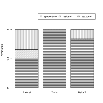
Figure 3: Proportion of the space-time, seasonal and residual components of the variance for each climate variable

		$\phi_{sp}$	$\phi_{ti}$	$\phi_{cy}$	$\eta$
$Y_{1}$	Est.	0.188	28.979	15.210	0.774
	(CI)	(0.184 0.192)	(28.871 29.072)	(14.972 15.394)	(0.774 0.775)
$Y_{2}$	Est.	0.138	9.628	10.176	0.943
	(CI)	(0.137 0.140)	(9.476 9.750)	(10.102 10.239)	(0.942 0.943)
$Y_{3}$	Est.	0.431	23.814	9.760	0.166
	(CI)	(0.429 0.432)	(23.576 23.995)	(9.690 9.835)	(0.165 0.168)
		$\sigma^{2}_{cy}$	$\sigma^{2}_{\epsilon}$	$\sigma^{2}_{\omega}$
$Y_{1}$	Est.	0.617	0.176	0.413
	(CI)	(0.612 0.623)	(0.175 0.178)	0.409 0.416)
$Y_{2}$	Est.	6.968	0.008	0.050
	(CI)	(6.830 7.092)	(0.008 0.008)	(0.050 0.051)
$Y_{3}$	Est.	2.799	0.062	0.525
	(CI)	(2.647 2.919)	(0.061 0.062 )	(0.519 0.532)

Table 3: Posterior estimates of the Gaussian process and annual cyclical component parameters, as in equations (5) and (4), respectively.

Table 3 shows a clear evidence that the three components are non-separable in space and time, as the $\eta$ parameter is never close to 0. The practical ranges and covariances of the three components provide useful information on the extent of the spatial, temporal and annual cyclical dependence. The spatial practical ranges of the process components are 15.95km ($Y_{1}$), 21.676km ($Y_{2}$) and 6.967km ($Y_{3}$), suggesting a much more localized behavior of the temperature range with respect to the other two variables. In terms of time dependence, we have the following practical ranges: 37.78 days ($Y_{1}$), 113.73 days ($Y_{2}$) and 45.98 days ($Y_{3}$). These values highlight the length of time windows of correlated behavior for each component, suggesting a similar temporal dependence for the rainfall and the temperature range. Finally the annual cyclical effect $\phi_{\mbox{cy}}$ (practical ranges: 71.99 days ($Y_{1}$), 107.60 days ($Y_{2}$), 112.19 days ($Y_{3}$)) highlights a similar behavior for the second and third variables, as expected: a shorter cycle is estimated for the rain, while annual cycles are longer and almost seasonal (4 months long) for both temperatures. Correlation between climate variables are also obtained and they are all significantly different from zero. Rain and minimum temperature are positively correlated (0.210 with a narrow 95$\%$ credible interval (0.208,0.213)), while rain an temperature range are negatively correlated (-0.214 with again a narrow 95$\%$ CI (-0.218,-0.211)). The minimum temperature and the temperature range are negatively correlated, showing a stronger relation, as expected (-0493, 95$\%$ CI (-0.499,-0.497)). This proposal allows to gather considerably more information on the joint behavior of the climate variables than previous studies where an older version of the database was also used to correlate climate data with altitude [11, 10].

In figure 4 examples of maps of two monthly effects of the annual cyclical components are reported. The maps for the months of January and August have been chosen as representative of the factors affecting the composition of ecosystems and their distribution over the Italian territory. Above all, these factors include moisture availability in the different seasons, winter cold and summer drought. Firstly, the model was able to show some interesting seasonal patterns of rainfall (fig. 4a and 4d). These include: (i) the continental regime of the Alpine Province, the only region with larger rainfall values in summer than in winter months; (ii) the transitional character of the Po Plain Province towards a more Mediterranean regime, with lower summer rainfall; (iii) the very clear latitudinal gradient in both the Apennine and peninsular Tyrrhenian Provinces, which mainly reflects the varying distance from the coast of the mountain reliefs. More local patterns are suggested as well, that however need a more in depth investigation at the Section and/or Subsection ecoregional levels. These include, for example, the longitudinal summer gradient in rainfall between Eastern and Western Alps and the marked summer rainfall decrease in some Southern peninsular and main island sectors. Secondly, winter cold (fig. 4b) clearly characterises both the Alpine and Po Plain Provinces within the Temperate Division. On the contrary, the variable behaviour within the Apennine Province should be further investigated in order to highlight in detail the differences with the Tyrrhenian Province of the Mediterranean Region. Patterns that need to be characterised at lower ecoregional levels emerged in this case as well. These include, for example, the latitudinal gradient along the Adriatic Province and the differences between the two main Tyrrhenian islands. The third component of the process, among the several features, highlights the relevance of reduced winter temperatures and their variation in characterising the termic continentality of the Po Plain and Adriatic Provinces. It also confirms that higher temperatures occur in both the Tyrrhenian and the Adriatic Mediterranean Provinces.

In tables 4 and 5 the posterior estimates of the intercepts and regression coefficients distinguished by ecoregion are reported. Remark that all estimates for the 4th ecoregion (1D) are not relevant and very different from the other values, due to the presence of only one monitoring station in the given area. This suggests to consider the aggregation of the 4th ecoregion to one of its neighbors for future investigations, as recently tested in the first report on the Italian natural capital. Estimates of the model intercepts $\beta_{0}$’s allow to analyse the behaviour of each component in the specific ecoregion. The only estimate that shows a value close to zero is for temperature range in ecoregion 1B, the Po Plain Province, suggesting a very small temperature range. All ecoregions are well characterized with some overlapping of credible intervals for each variable, suggesting similarities between areas. Similar behavior in terms of rainfall ($Y_{1}$) can be found in ecoregions 1B, 2A, 2B and 2C ($j=2,5,6,7$), while 1A, 1B and 2C ($j=1,2,7$) show similarities in terms of minimum temperature ($Y_{2}$) and only 1A and 2C ($j=1,7$) show intervals estimates overlapping for the temperature range ($Y_{3}$). Notice that 1B covering the Po Plain is a very variable area where a transition from the continental to the mediterranean behaviours occurs. The relation with the elevation described by the estimates of the regression coefficients $\beta_{1}$’s often admits the zero value in the 95$\%$ credible interval. This is likely linked to the presence of a latitudinal gradient in the area. For example, in the Po Plain Province (1B) a large area is divided by the Po river in a northern sector with continental regime and a southern sector with Apennine regime, as already highlighted for the effects of the cyclical components. The Alpine province (1A) is associated to regression coefficients that are all quite far from zero and this can be linked to the absence of a latitudinal gradient, being the region affected only by a longitudinal variation. Moreover the area is characterized by a considerable relief energy (large quota gradient).

		$\beta_{0,1}$	$\beta_{0,2}$	$\beta_{0,3}$	$\beta_{0,4}$
$Y_{1}$	Est.	1.348	0.741	0.965	-0.050
	(CI)	(1.280 1.400)	(0.668 0.794)	(0.924 1.003)	(-8.155 7.777)
$Y_{2}$	Est.	0.207	0.225	0.094	-0.005
	(CI)	(0.189 0.234)	(0.207 0.240)	(0.084 0.106)	(-1.746 1.758)
$Y_{3}$	Est.	0.155	0.008	0.779	0.083
	(CI)	(0.055 0.201 )	(-0.069 0.097)	(0.737 0.844)	(-4.919 4.748)
		$\beta_{0,5}$	$\beta_{0,6}$	$\beta_{0,7}$
$Y_{1}$	Est.	0.633	0.740	0.783
	(CI)	(0.520 0.787)	(0.710 0.774)	(0.745 0.838)
$Y_{2}$	Est.	0.878	0.457	0.277
	(CI)	(0.838 0.910)	(0.445 0.464)	(0.263 0.295)
$Y_{3}$	Est.	-1.965	-0.070	0.196
	(CI)	(-2.038 -1.856)	(-0.125 -0.038)	(0.127 0.264)

Table 4: Point estimates of the intercepts at each ecoregion and for each Gaussian process component. Ecoregions are coded as follows $1=1A$, $2=1B$, $3=1C$, $4=1D$, $5=2A$, $6=2B$ and $7=2C$.

		$\beta_{1,1}$	$\beta_{1,2}$	$\beta_{1,3}$	$\beta_{1,4}$
$Y_{1}$	Est.	0.029	0.498	0.248	63.022
	(CI)	(-0.022 0.068)	(0.189 0.742)	(0.208 0.294)	(-650.237 788.956)
$Y_{2}$	Est.	-0.747	-0.322	-0.452	73.423
	(CI)	(-0.761 -0.729)	(-0.414 -0.242)	(-0.470 -0.437)	(-86.057 231.301)
$Y_{3}$	Est.	-0.366	-0.094	-1.073	-117.311
	(CI)	(-0.428 -0.305)	(-0.648 0.423)	(-1.177 -1.023)	(-544.667 338.024)
		$\beta_{1,5}$	$\beta_{1,6}$	$\beta_{1,7}$
$Y_{1}$	Est.	-0.532	0.548	0.416
	(CI)	(-1.250 0.241)	(0.502 0.592)	(0.272 0.546)
$Y_{2}$	Est.	-2.802	-0.842	-0.452
	(CI)	(-3.038 -2.541)	(-0.856 -0.826)	(-0.498 -0.405 )
$Y_{3}$	Est.	8.256	0.040	-0.736
	(CI)	(6.891 9.607)	(-0.042 0.112)	(-0.985 -0.570)

Table 5: Point estimates of the regression coefficients$\times 1000$ at each ecoregion and for each Gaussian process component. Ecoregions are coded as follows $1=1A$, $2=1B$, $3=1C$, $4=1D$, $5=2A$, $6=2B$ and $7=2C$.

After model fitting, we used posterior samples to predict the values of the three variables over a $15Km\times 15km$ grid of 3305 spatial points over 720 times. Posterior estimates of each time series were obtained in only 20 minutes on the TeraStat cluster [18] that allows for fast computing with a limitation on the number of processes that can be lunched simultaneously. Such limitation is not implemented at the Bari ReCaS DataCenter that provides a computing power of 128 servers each with 64 cores and 256GB of RAM. It houses a small cluster dedicated to High Performance Computing, running applications using many cores at the same time, that was used for parallel computing of the predictions. To asses the out of sample predictive capability of the chosen model, we built a validation set starting with the finest definition of ecoregions ($k=5$, 35 ecoregions). We selected 10$\%$ of the available observations with at least one station per ecoregion, excluding ecoregions with only one station (1A1a,1D1a). The validation set was used to evaluate the root mean squared prediction error for each response variable on its original scale, obtaining very encouraging results: Rain 5.8mm, T. min 1.3^∘, T. max 1.4^∘ corresponding to a relative error of 0.38% for the Rain, 2.64% and 2.47% for the maximum and minimum temperature respectively.

5 Concluding remarks and future developments

In this paper we present a multivariate generalization of the NNGP model proposed in Datta et al. [16]. Our model combines the computational efficiency of NNGP’s with several new ideas for handling complex structures typical of climate variables. We use the linear model of coregionalization to account for multivariate spatio-temporal dependencies, a circular representation of the time index to define the annual cycles and propose an efficient implementation of the NNGP that allows to estimate the model with a huge amount of data. Results are very encouraging as we are able to interpolate climate variables at any spatial and temporal resolution and impute missing values. The richness of model output allows to characterise the Italian ecoregions with respect to rainfall, minimum and maximum temperature returning information on cyclical trend, spatial and temporal correlation.

The future will find us working on more detailed bioclimatic characterisation of the Italian ecoregions. To do that we need to obtain parameter estimates for all the available ecoregional tiers, including Divisions, Sections and Subsections. We are interested in better understanding the role of climate variables at a more detailed ecoregion level. Further, as new ecoregional boundaries have recently been proposed mainly based on biogeographic and physiographic considerations (Blasi et al., unpublished data), the model could be applied to develop a climatic characterisation of the new strata, comparing results to those reported in this paper.

References

- Bai et al. [2012] Bai, Y., Song, P. X.-K., and Raghunathan, T. E. (2012). Joint composite estimating functions in spatiotemporal models. Journal of the Royal Statistical Society: Series B (Statistical Methodology), 74(5), 799–824.
- Bailey [1983] Bailey, R. G. (1983). Delineation of ecosystem regions. Environmental Management, 7(4), 365–373.
- Bailey [2004] Bailey, R. G. (2004). Identifying ecoregion boundaries. Environmental Management, 34(Suppl 1), S14–S26.
- Banerjee et al. [2014] Banerjee, S., Gelfand, A. E., and Carlin, B. P. (2014). Hierarchical Modeling and Analysis for Spatial Data. Chapman and Hall/CRC, New York, second edition.
- Bevilacqua et al. [2012] Bevilacqua, M., Gaetan, C., Mateu, J., and Porcu, E. (2012). Estimating space and space-time covariance functions for large data sets: A weighted composite likelihood approach. Journal of the American Statistical Association, 107(497), 268–280.
- Bevilacqua et al. [2016a] Bevilacqua, M., Alegria, A., Velandia, D., and Porcu, E. (2016a). Composite likelihood inference for multivariate gaussian random fields. Journal of Agricultural, Biological, and Environmental Statistics, 21(3), 448–469.
- Bevilacqua et al. [2016b] Bevilacqua, M., Fassò, A., Gaetan, C., Porcu, E., and Velandia, D. (2016b). Covariance tapering for multivariate gaussian random fields estimation. Statistical Methods & Applications, 25(1), 21–37.
- Blangiardo and Cameletti [2015] Blangiardo, M. and Cameletti, M. (2015). Spatial and Spatio-temporal Bayesian Models with R - INLA. Wiley.
- Blangiardo et al. [2013] Blangiardo, M., Cameletti, M., Baio, G., and Rue, H. (2013). Spatial and spatio-temporal models with r-inla. Spatial and Spatio-temporal Epidemiology, 7, 39 – 55.
- Blasi et al. [2007a] Blasi, C., Michetti, L., Del Moro, M. A., Testa, O., and Teodonio, L. (2007a). Climate change and desertification vulnerability in southern italy. Phytocoenologia, 37(3-4), 495–521.
- Blasi et al. [2007b] Blasi, C., Chirici, G., Corona, P., Marchetti, M., Maselli, F., and Puletti, N. (2007b). Spazializzazione di dati climatici a livello nazionale tramite modelli regressivi localizzati. Forest@, 4, 213–219.
- Blasi et al. [2014] Blasi, C., Capotorti, G., Copiz, R., Guida, D., Mollo, B., Smiraglia, D., and Zavattero, L. (2014). Classification and mapping of the ecoregions of italy. Plant Biosystems - An International Journal Dealing with all Aspects of Plant Biology, 148(6), 1255–1345.
- Cressie and Wikle [2011] Cressie, N. and Wikle, C. K. (2011). Statistics for Spatio-Temporal Data. Wiley, Hoboken, N.J.
- Cressie et al. [2010] Cressie, N., Shi, T., and Kang, E. L. (2010). Fixed rank filtering for spatio-temporal data. Journal of Computational and Graphical Statistics, 19(3), 724–745.
- Datta et al. [2016a] Datta, A., Banerjee, S., Finley, A. O., and Gelfand, A. E. (2016a). Hierarchical nearest-neighbor gaussian process models for large geostatistical datasets. Journal of the American Statistical Association, 111(514), 800–812.
- Datta et al. [2016b] Datta, A., Banerjee, S., Finley, A. O., Hamm, N. A. S., and Schaap, M. (2016b). Nonseparable dynamic nearest neighbor gaussian process models for large spatio-temporal data with an application to particulate matter analysis. Ann. Appl. Stat., 10(3), 1286–1316.
- Eidsvik et al. [2014] Eidsvik, J., Shaby, B. A., Reich, B. J., Wheeler, M., and Niemi, J. (2014). Estimation and prediction in spatial models with block composite likelihoods. Journal of Computational and Graphical Statistics, 23(2), 295–315.
- Ferraro Petrillo and Raimato [2014] Ferraro Petrillo, U. and Raimato, G. (2014). Terastat computer cluster for high performance computing. “http://www.dss.uniroma1.it/en/node/6554” Department of Statistical Science Sapienza university of Rome.
- Fick and Hijmans [2017] Fick, S. E. and Hijmans, R. J. (2017). Worldclim 2: new 1-km spatial resolution climate surfaces for global land areas. International Journal of Climatology, pages n/a–n/a.
- Finley et al. [2012] Finley, A. O., Banerjee, S., and Gelfand, A. E. (2012). Bayesian dynamic modeling for large space-time datasets using gaussian predictive processes. Journal of Geographical Systems, 14(1), 29–47.
- Gelfand et al. [2010] Gelfand, A., Diggle, P., Fuentes, M., and Guttorp, P. (2010). Handbook of Spatial Statistics. Chapman and Hall.
- Gelfand et al. [2004] Gelfand, A. E., Schmidt, A. M., Banerjee, S., and Sirmans, C. F. (2004). Nonstationary multivariate process modeling through spatially varying coregionalization. TEST, 13(2), 263–312.
- Gneiting [2002] Gneiting, T. (2002). Nonseparable, Stationary Covariance Functions for Space-Time Data. Journal of the American Statistical Association, 97(458), 590–600.
- Gopar-Merino et al. [2015] Gopar-Merino, L. F., Velázquez, A., and de Azcárate, J. G. (2015). Bioclimatic mapping as a new method to assess effects of climatic change. Ecosphere, 6(1), 1–12. art13.
- Hijmans et al. [2005] Hijmans, R. J., Cameron, S. E., Parra, J. L., Jones, P. G., and Jarvis, A. (2005). Very high resolution interpolated climate surfaces for global land areas. International Journal of Climatology, 25(15), 1965–1978.
- Jona Lasinio et al. [2013] Jona Lasinio, G., Mastrantonio, G., and Pollice, A. (2013). Discussing the “big n problem”. Statistical Methods and Applications, 22(1), 97–112.
- Katzfuss and Cressie [2012] Katzfuss, M. and Cressie, N. (2012). Bayesian hierarchical spatio-temporal smoothing for very large datasets. Environmetrics, 23(1), 94–107.
- Li et al. [2016] Li, S., Dragicevic, S., Castro, F. A., Sester, M., Winter, S., Coltekin, A., Pettit, C., Jiang, B., Haworth, J., Stein, A., and Cheng, T. (2016). Geospatial big data handling theory and methods: A review and research challenges. ISPRS Journal of Photogrammetry and Remote Sensing, 115, 119 – 133. Theme issue ’State-of-the-art in photogrammetry, remote sensing and spatial information science’.
- Lindgren et al. [2011] Lindgren, F., Rue, H., and Lindström, J. (2011). An explicit link between gaussian fields and gaussian markov random fields: the stochastic partial differential equation approach. Journal of the Royal Statistical Society: Series B (Statistical Methodology), 73(4), 423–498.
- Loveland and Merchant [2004] Loveland, T. R. and Merchant, J. M. (2004). Ecoregions and ecoregionalization: Geographical and ecological perspectives. Environmental Management, 34((Suppl 1): S1).
- McKenney et al. [2010] McKenney, D. W., Pedlar, J. H., Lawrence, K., Gray, P. A., Colombo, S. J., and Crins, W. J. (2010). Current and projected future climatic conditions for ecoregions and selected natural heritage areas in ontario. Technical Report CCRR-16, Climate Change Research Report-Ontario Forest Research Institute.
- Metzger et al. [2013] Metzger, M. J., Bunce, R. G. H., Jongman, R. H. G., Sayre, R., Trabucco, A., and Zomer, R. (2013). A high-resolution bioclimate map of the world: a unifying framework for global biodiversity research and monitoring. Global Ecology and Biogeography, 22(5), 630–638.
- Mücher et al. [2010] Mücher, C. A., Klijn, J. A., Wascher, D. M., and Schaminée, J. H. (2010). A new european landscape classification (lanmap): A transparent, flexible and user-oriented methodology to distinguish landscapes. Ecological Indicators, 10(1), 87 – 103. Landscape Assessment for Sustainable Planning.
- Pesaresi et al. [2014] Pesaresi, S., Galdenzi, D., Biondi, E., and Casavecchia, S. (2014). Bioclimate of italy: application of the worldwide bioclimatic classification system. Journal of Maps, 10(4), 538–553.
- Rue and Held [2005] Rue, H. and Held, L. (2005). Gaussian Markov Random Fields: Theory And Applications. Monographs on Statistics and Applied Probability. Chapman and Hall/CRC.
- Rue et al. [2009] Rue, H., Martino, S., and Chopin, N. (2009). Approximate bayesian inference for latent gaussian models by using integrated nested laplace approximations. Journal of the Royal Statistical Society: Series B (Statistical Methodology), 71(2), 319–392.
- Shirota and Gelfand [2017] Shirota, S. and Gelfand, A. E. (2017). Space and circular time log gaussian cox processes with application to crime event data. Ann. Appl. Stat., 11(2), 481–503.
- Spiegelhalter et al. [2002] Spiegelhalter, D. J., Best, N. G., Carlin, B. P., and Van Der Linde, A. (2002). Bayesian measures of model complexity and fit. Journal of the Royal Statistical Society: Series B (Statistical Methodology), 64(4), 583–639.
- Xu et al. [2015] Xu, G., Liang, F., and Genton, M. G. (2015). Bayesian spatio-temporal geostatistical model with an auxiliary lattice for large datasets. Statistica Sinica, 25, 61–79.