Radially falling test particle approaching an evaporating black hole

Abstract

A simple model for an evaporating non-rotating black hole is considered, employing a global time that does not become singular at the putative horizon. The dynamics of a test particle falling radially towards the center of the black hole is then investigated. Contrary to a previous approach, we find that the particle may pass the Schwarzschild radius before the black hole has gone. Backreaction effects of Hawking radiation on the space-time metric are not considered, rather a purely kinematical point of view is taken here. The importance of choosing an appropriate time coordinate when describing physical processes in the vicinity of the Schwarzschild radius is emphasized. For a shrinking black hole, the true event horizon is found to be inside the sphere delimited by that radius.

I Introduction

In a recent article in this journal,aste05 Aste and Trautmann discussed the radial fall of a test particle onto a black hole evaporating by Hawking radiation. They did so in terms of what they admit to be a toy model, an approximation the validity of which is, in their own words, “dubious at best” near the event horizon of the black hole. Nevertheless, they believe their model to be a good approximation far from the horizon and consider their major qualitative result to be correct, i.e., that the black hole will evaporate under an infalling particle or observer before the latter can cross the horizon. Such a result would call into question that a black hole can form at all vachaspati07 , because any piece of infalling matter should hover above the nascent horizon, accumulating time dilation, while the incipient black hole is already busy evaporating.

The purpose of this paper is to show that a slightly more realistic approach, still a toy model, but at least one using a time coordinate that does not become singular at the Schwarzschild radius, leads to a diametrically opposed prediction: an observer falling towards an evaporating black hole will normally cross the “horizon” without noticing anything dramatic happening and, unfortunately, hit the central singularity the same way as with an eternal black hole. Rather precise timing of the fall, approaching the black hole near the end of its lifetime, when its mass has gotten small, would be necessary to avoid hitting it before it evaporates. Moreover, the Schwarzschild radius of an evaporating black hole loses its property of being an event horizon. Rather, its behavior bears some similarities to that of the Hubble sphere in cosmology,davis04 the locus of galaxies receding from an observer at the speed of light: a light signal sent outward from the Schwarzschild radius or even from slightly inside it can reach outside observers due to the shrinking of the radius.

These conclusions seem to be at odds not only with Ref. [aste05, ] but also with [vachaspati07, ], who use a genuine quantum mechanical formalism. However, the calculations in Ref. [vachaspati07, ] are based on the Schwarzschild time coordinate and therefore subject to the restrictions imposed by its use, even if this does not show up in a divergence of the calculation. We will discuss the nature and operational meaning of different time coordinates in Sec. 2. As we shall see, time coordinates constructed in an analogous way to the Schwarzschild time must become infinite for events on a horizon or one-way membrane for light propagation. If a quantum mechanical Hamiltonian is chosen conjugate to this time coordinate, it will obviously not be able to capture any dynamics at the horizon, whether or not this is signaled by an explicit divergence. Using this time automatically imposes limitations on the range of the description in a way not required by some other time coordinates. These restrictions then may lead to a misinterpretation of mathematically correct results.

The calculations in this paper are purely classical, i.e., no attempt is made at a quantum mechanical model of the radiation. There are controversial statements in the literature about the effects of backreaction of Hawking radiation. While there seems to be general agreement that the emission of Hawking radiation begins already during the collapse of a star, i.e., before the formation of an event horizon, some authors gerlach76 ; mersini14 ; peiming16 believe that the ensuing reduction of mass-energy may prevent the formation of a horizon altogether, whereas others parentani94 ; paranjape09 ; modak14 insist that it is too small to have such a drastic effect. We will not tackle these questions which refer to the dynamics of black-hole formation. Rather, the focus will be on getting the kinematics right, which, as I argue here, necessitates to avoid using a time coordinate that is singular at the apparent horizon. In the conclusions, I will return to the question whether we may learn something regarding the aforementioned controversy from our results as well. In any case, the Aste-Trautmann calculation does not take backreaction effects into account and nevertheless predicts evaporation of a black hole from under the feet of an infalling observer, so to speak. An attempt to improve a little on this calculation therefore need not invoke backreactions either.

The remainder of this paper is organized as follows. In Sec. II, Painlevé-Gullstrand (PG) coordinates for the metric of an eternal spherically symmetric black hole are introduced besides the standard Schwarzschild ones. Ways to operationally realize the synchronies established by these coordinates are presented and the reason for the singularity of standard Schwarzschild coordinates at the event horizon is explained. It is shown that in PG coordinates not only does the proper time of a particle falling into the black hole remain finite but also the global time. Section III briefly recalls the model of an evaporating black hole introduced by Aste and Trautmann and gives an alternative model based on a similar construction but now using the PG time coordinate to describe the decay law due to Hawking radiation. The equations of motion for a particle falling radially towards the black hole are given for this model and simplified. Finally, in Sec. IV, these equations as well as those describing outgoing light rays are solved numerically. The black hole does not normally evaporate, before an infalling object passes the Schwarzschild radius. A summary and conclusions are given in Sec. V.

II Time in general relativity

Our concept of time has been radically altered by the relativity theories. Just how radical the nature of this change turns out to be, may not have been as well appreciated as the wide acceptance of these theories would suggest.

Newton believed in absolute time as an independent aspect of reality. Newtonian simultaneity is objective. It can be ascertained, in principle, by the fact that there is no limit to the speed of signals in Newtonian physics. The motion of the center of mass of an object will immediately affect its gravitational interaction with a distant detector.

Einstein first deprived time of its absolute character in special relativity (SR), where different observers may have different notions of simultaneity, and later reduced it to a mere coordinate of four-dimensional spacetime, in general relativity (GR). The only concept of a physical time surviving in GR is that of proper time which is only local.

Already in his paper introducing SR,einstein05 Einstein emphasized that his approach to synchronization of clocks and, hence, simultaneity, was a definition, a fact that he later accentuated by stating that the constancy of the speed of light underlying his notion of simultaneity was “neither a supposition nor a hypothesis about the nature of light but a stipulation.”einstein52

That is, one may define simultaneity via the Einstein synchronization procedure (using light signals and defining the time of a distant event as the average between the times of emission and back reception of a light signal sent from the world line of an observer to the event and immediately reflected back), but this is in no way compulsory! There is a (gauge) degree of liberty in establishing synchrony of distant clocks,rizzi04a due to the fact that there is a finite maximum speed of signal transport. This prevents us from producing a unique standard of simultaneity of distant events. All we can distinguish objectively is whether pairs of such events are timelike, null or spacelike.

Nevertheless, the idea still appears to be ingrained in many minds that, once we have fixed an observer, what is simultaneous at a distance for this particular observer is objective, which would mean that a global “physical” time could be established at least for inertial observers. That this is incorrect often does not seem to be appreciated, and for a reason. If we extend the proper times of inertial observers via Einstein synchronization to global time coordinates for each of them (which is possible in a flat spacetime), this brings out the equivalence of all inertial systems stated in the relativity principle and renders the Lorentz symmetry of nature manifest. Therefore, as long as we are dealing, in SR, with (global) inertial systems only, Einstein synchronization is preferable over all other synchronization methods on practical grounds.

On the other hand, when we are concerned with non-inertial systems, then different synchronization methods may sometimes be preferable even in SR. Different standard clocks fixed on the rim of a rotating circular disk run at the same rate as viewed from an observer at the center of the disk. Nevertheless, if one synchronizes them around the rim with the Einstein procedure, a time gap will appear between the clock at the starting point, at angular position $\varphi$ and the one at angle $\varphi+2\pi$,kassner12b i.e., at the same position after having performed the synchronization procedure for a full turn. Setting clocks at fixed radial distance by a light signal from the center of the disk insteadcranor99 (“central synchronization”) leads to a simple description of phenomena such as the Sagnac effect, but gives rise to direction-dependent velocities of light.kassner12b

Obviously, practitioners of general relativity are less prone to falling into the trap of absolutizing observer-conditioned simultaneity, knowing that simultaneity at a distance is just a matter of choice of an appropriate spacelike foliation of spacetime (assuming one exists). There are clearly different choices, even for a specific observer. And, of course, this is true in SR as well, which can easily be given a covariant formulation. The mathematics is that of GR with vanishing Riemannian curvature. Therefore, the same freedom of establishing “sheets of simultaneity” exists in SR as in GR.

Global times in GR are just time coordinates. Generally, it is not possible to extend the proper time of an observer to a global coordinate in a way preserving its property of being the proper time for local observers at different positions, because that would lead to coordinate singularities in curved spacetime. To be able to interpret the coordinate in question as a time, its surfaces of constant value should of course be spacelike.

After these preliminaries, consider a standard representation of the metric of a Schwarzschild black hole,

$$\mathrm{d}s^{2}=\left(1-\frac{r_{s}}{r}\right)c^{2}\mathrm{d}t_{S}^{2}-\left(1-\frac{r_{s}}{r}\right)^{-1}\mathrm{d}r^{2}-r^{2}\mathrm{d}\Omega^{2}\>,$$ (1)

where $r_{s}=2GM_{0}/c^{2}$ is the Schwarzschild radius. $M_{0}$ is the mass of the black hole, while $G$ is Newton’s gravitational constant and $c$ is the speed of light. $\mathrm{d}\Omega^{2}=\mathrm{d}\vartheta^{2}+\sin^{2}\vartheta\mathrm{d}\varphi^{2}$ is the squared line element on the surface of a unit sphere, and we have given the time coordinate a subscript $S$ to distinguish it from alternative ones.

How is the time coordinate in the metric (1) constructed? It is not the proper time of any observer stationary within the metric, except for those at infinity. This can be seen immediately via calculation of the proper time interval $d\tau$ for such an observer ($\mathrm{d}s^{2}=c^{2}\,\mathrm{d}\tau^{2}$). Assuming $\mathrm{d}r=\mathrm{d}\vartheta=\mathrm{d}\varphi=0$, we find

$$\mathrm{d}\tau=\sqrt{1-\frac{r_{s}}{r}}\mathrm{d}t_{S}\>.$$ (2)

This is not a total differential, so this proper time cannot be integrated to provide us with a global time coordinate. However, local clocks at a radial distance $r$ from the center can be made to run fast by a factor of $\left(1-\frac{r_{s}}{r}\right)^{-1/2}$ with respect to local standard clocks. Presently, we will not consider the case $r<r_{s}$. For a discussion of how observers may determine that they are at rest within the spacetime described by the metric (1), see Ref. [misner73, ]. Once nonstandard clocks running at the same rate have been established, we only have to synchronize them, i.e., to fix the offset of each clock. The synchronization procedure leading to the time $t_{S}$ (up to a constant offset) is Einstein synchronization, based on the requirement that the time a light signal takes to travel from an observer $A$ to an observer $B$ is the same as the time it takes from $B$ to $A$. Note that this is valid with the Schwarzschild time, even though the coordinate speed of light is neither equal to $c$ nor constant. Light propagation is described by $\mathrm{d}s^{2}=0$, which for $\mathrm{d}\vartheta=\mathrm{d}\varphi=0$ leads to $\mathrm{d}r/\mathrm{d}t_{S}=\pm\left(1-r_{s}/r\right)c$, and the coordinate velocities of light in the $\vartheta$ and $\varphi$ directions also just change sign when switching from the forward to the backward direction: $r\,\mathrm{d}\vartheta/\mathrm{d}t_{S}=\pm\sqrt{1-r_{s}/r}\,c$, $r\sin\vartheta\,\mathrm{d}\varphi/\mathrm{d}t_{S}=\pm\sqrt{1-r_{s}/r}\,c$. All that matters for Einstein synchronization to work, is that the speed of light is the same in both directions at any point along a spatial path. This is guaranteed for any diagonal metric with time-independent coefficients, i.e., a static metric. If the metric is only diagonal, Einstein synchronization is normally still possible locally, i.e., for close-by clocks, because the property that the vacuum speed of light does not depend on the direction along a path is still satisfied on any one of its infinitesimal pieces. But in the case where we do not have fixed time-dilation factors that depend on position only, clocks will have to be constantly resynchronized with their neighbours, in order to operationally construct the time coordinate. It is not sufficient to just synchronize them once and let them run at a fixed prescribed rate.

The spatial coordinate $r=r_{s}$ describes the event horizon, whenever it is part of the solution, i.e., when the whole spherically symmetric mass distribution, outside of which the metric (1) holds, does not extend beyond $r_{s}$. Let us now ask what time coordinates we may assign to events on the horizon operationally via Einstein synchronization. Light cannot return to a distant observer from the horizon. Stated in a highbrow way, it takes an infinite time to return. Since by definition the time to go to the horizon must be the same as the time to return, both times must be infinite. So the only time coordinate possible for the horizon is $\infty$. There are no events at finite time on it, even for an eternal black hole. This is just another way of expressing the fact that Schwarzschild coordinates become singular at the horizon.

Note that we may generalize this observation: Any time-orthogonal coordinate system describing a spacetime, in which coordinate stationary observers stay outside an event horizon that may be present, will have to assign infinite time to the horizon, so the coordinates must be singular there.

Folklore has it that an observer, starting at a finite distance from a black hole and falling towards it, will reach the event horizon in finite proper time but take an infinite amount of time to reach it “from the perspective of a distant observer”. The first of these two statements is certainly true and also has a pretty clear physical meaning, because proper time is something the infaller can read off his standard clock. The second statement refers to Schwarzschild time and is also correct, if properly understood. Unfortunately, it is often misunderstood, then leading to misconceptions such as that the infalling observer may, just before she crosses the horizon, see the whole future of the universe or else that the collapse of a star will halt due to time dilation, before matter can cross the “critical radius”.spivey15

While the first of these beliefs is simply wrong,grib09 the second may be traced to mistaking the Schwarzschild time for a “coordinate independent physical quantity”,spivey15 an idea that is fully antithetical to GR, in which the Schwarzschild time merely is a coordinate. Its diverging at the horizon does not mean that the temporal end of the universe is approached. The event in spacetime corresponding to the arrival of an infaller at the horizon is in no way singular. There is time after and there is space around.

For an eternal black hole, described by the Schwarzschild metric (1), it is easy to see that $t_{S}$ cannot be a physical time near the event horizon. First, isotropy and invariance under time translations show that all points on the horizon are equivalent. Therefore, we expect events to exist on the horizon at all physical times (this may be taken as the meaning of eternal existence). But a Kruskal-Szekeres diagram readily shows that, if we exclude the origin (where the behavior of the Schwarzschild time is similar to that of the angular polar coordinate near the origin of a Euclidean coordinate system, in being undefined and arbitrary) the horizon has only one Schwarzschild time, viz. $t_{S}=\infty$, even though it occupies an infinite 3D submanifold of spacetime. Therefore, interpreting the Schwarzschild time as a physical time meets some difficulties on the horizon and in its immediate neighbourhood.

Moreover, the statement that the infaller takes infinite time as seen from a distant observer is largely devoid of physical meaning. What it means is essentially that it is possible to establish a simultaneity relation so that the time coordinate of the distant observer that is simultaneous with the event of the infaller touching the horizon is infinite. But this again is just a statement about coordinates. There may be, and as we shall see, there are, choices of time coordinates so that the event of the infaller on the horizon is simultaneous with a finite time of the distant observer. Translated to the sloppy language of folklore, this would say that the infaller reaches the horizon in a finite time from the perspective of a distant observer. This is equally correct as the original statement, it just refers to a different time coordinate, that, incidentally, may become equal to the proper time of a stationary observer at sufficiently large $r$ the same way as the Schwarzschild time does.

What residual of physical meaning we can assign to the fact that the Schwarzschild time diverges on approach to the horizon is that if an event outside the horizon is in timelike relationship to an observer just crossing the horizon, it must be in her causal past. Differently stated, events outside the horizon that are not in the causal past of an event on the horizon, must be spacelike with respect to it, they cannot be in its timelike causal future. But this is obvious from the fact that the timelike future of any event on the horizon is only inside it, ending in the singularity.

A major disadvantage of the Schwarzschild time coordinate is that it does not give us, without calculation, a time value, beyond which we know any signal emitted by the distant observer to be unable to reach an infalling observer. According to Schwarzschild simultaneity, any external signal is sent before the horizon is reached by the hapless infaller, so we always have to do a calculation to determine whether it may or may not reach her.

Let us consider a different form of the Schwarzschild metric:

$$\mathrm{d}s^{2}=\left(1-\frac{r_{s}}{r}\right)c^{2}\mathrm{d}t^{2}-2\sqrt{\frac{r_{s}}{r}}\,c\,\mathrm{d}t\mathrm{d}r-\mathrm{d}r^{2}-r^{2}\mathrm{d}\Omega^{2}\>.$$ (3)

These are Painlevé-Gullstrand coordinatespainleve21 ; gullstrand22 and they are known to be continuous across the horizon. The spatial coordinates are the same as in (1), the time coordinate $t$, to which I will refer as the Painlevé-Gullstrand or PG time, is related to the Schwarzschild time by

$$c\,t=c\,t_{S}+2\sqrt{rr_{s}}-r_{s}\ln\frac{\sqrt{r}+\sqrt{r_{s}}}{\sqrt{r}-\sqrt{r_{s}}}+c\,t_{R}\>,$$ (4)

where $t_{R}$ is an arbitrary constant that can be chosen to make the two times equal at some fixed radius $R$. Since the two metrics (1) and (3) are related by a coordinate transformation, they describe the same patch of spacetime in their common domain. The coordinate transformation (4) is what may be called a synchronization transformation, because the two times $t$ and $t_{S}$ run at the same rate for a coordinate stationary observer at $r$, their only difference being a fixed albeit $r$ dependent offset. Not every function of $r$ is eligible as an offset, i.e., will lead to an acceptable new time coordinate. If we write

$$c\,\mathrm{d}t=c\,\mathrm{d}t_{S}+f^{\prime}(r)\mathrm{d}r$$ (5)

and assume $\mathrm{d}t_{S}$ to be the positive time interval light takes to cover the radial distance $\mathrm{d}r$, then $\mathrm{d}t$ must be positive as well. Since

$$c\,\mathrm{d}t_{S}=\left(1-\frac{r_{s}}{r}\right)^{-1}\left\lvert\mathrm{d}r\right\rvert$$ (6)

outside the horizon ($\mathrm{d}s^{2}=0$, $\mathrm{d}\vartheta=\mathrm{d}\varphi=0$), we obtain, for $r>r_{s}$ the inequality

$$\left\lvert f^{\prime}(r)\right\rvert<\left(1-\frac{r_{s}}{r}\right)^{-1}$$ (7)

as a condition for legitimate synchronization transformations. From (4), we find

$$f^{\prime}(r)=\sqrt{\frac{r_{s}}{r}}\left(1-\frac{r_{s}}{r}\right)^{-1}\>,$$ (8)

so the inequality is obviously satisfied for $r>r_{s}$, demonstrating that $t$ is a legitimate time coordinate outside the horizon, preserving the time ordering of the Schwarzschild time. Inside the horizon, the continuity of the PG time across $r=r_{s}$ suggests that it is a more acceptable time coordinate than the Schwarzschild time $t_{S}$. In fact, it is known that inside the horizon $t_{S}$ takes on the signature of a spatial coordinate (while the prefactor of $\mathrm{d}r$ in (1) becomes positive, suggesting time like nature), so it is not a trustworthy temporal coordinate anymore.

Sometimes the metric (3) is considered describing a frame of freely falling observers (rain frame), because the local time axis of the coordinate system is parallel to that of such an observer described in local Minkowski coordinates. However, this is rather a matter of interpretation than one of fact. The coordinate stationary observers of the Painlevé-Gullstrand form of the metric are precisely the same as those of its Schwarzschild form.

It is useful to have a look at a radially freely falling particle in this metric. Equations of motion can be obtained from the Lagrangian $L=\left(\dfrac{\mathrm{d}s}{\mathrm{d}\tau}\right)^{2}$, and setting $\mathrm{d}\vartheta=\mathrm{d}\varphi=0$, we need only two of them. Denoting derivatives with respect to the proper time of our observer by a dot, we may use the fact that $t$ is a cyclic coordinate and the definition of $L$ itself:

$$\frac{1}{2}\frac{\partial L}{\partial\dot{t}} =\left(1-\frac{r_{s}}{r}\right)c\dot{t}-\sqrt{\frac{r_{s}}{r}}\,\dot{r}=A=\text{const.}\>,$$ (9)

$$L =c^{2}=\left(1-\frac{r_{s}}{r}\right)c^{2}\dot{t}^{2}-2\sqrt{\frac{r_{s}}{r}}c\dot{t}\dot{r}-\dot{r}^{2}\>.$$ (10)

Requiring the particle to have a kinetic energy that would put it in a coordinate stationary state at infinity, i.e., $\lim_{r\to\infty}\dot{r}=0$, we can determine $A$:

$$c^{2}=c^{2}\dot{t}^{2}\big{|}_{r=\infty}\quad \Rightarrow\quad\dot{t}\big{|}_{r=\infty}=1$$

$$A=c\dot{t}\big{|}_{r=\infty}\quad \Rightarrow\quad A=c\>.$$ (11)

We may then insert $\dot{r}=\sqrt{\dfrac{r}{r_{s}}}\left[\left(1-\dfrac{r_{s}}{r}\right)c\dot{t}-c\right]$ from (9) into Eq. (10), which reduces to a quadratic equation for $\dot{t}$:

$$\dot{t}^{2}-\frac{2}{1-r_{s}/r}\dot{t}+\frac{1+r_{s}/r}{1-r_{s}/r}=0\>$$ (12)

with the solutions

$$\dot{t}=\begin{cases}1&\text{for }\dot{r}<0\\ \dfrac{1+r_{s}/r}{1-r_{s}/r}&\text{for }\dot{r}>0\end{cases}\>.$$ (13)

This immediately suggests an operational procedure for clock synchronization in the Painlevé-Gullstrand frame of reference. Local stationary clocks must be nonstandard, as they must run at the same rate as Schwarzschild clocks ($\partial t/\partial t_{S}=1$). Then to synchronize these clocks along a radial line, a standard clock, initialized to the time of, say an observer at $R$, should be tossed towards the center from that observer’s position with initial velocity $\dot{r}=-\sqrt{\dfrac{r_{s}}{R}}c$ (which turns out to be the same as $\dfrac{\mathrm{d}r}{\mathrm{d}t}$ here). Each stationary clock passed by the falling clock should be set to the time displayed by the latter the moment of its passage. This way all of them will be synchronized with the time $t$ of the observer at $R$, because with these initial conditions $\dot{t}=1$ according to Eq. (13). Clocks on a shell with fixed radius $r$ may be synchronized with one already set at this radius via Einstein synchronization, providing the light path is kept at constant $r\>$ (or else by having a clock fall from radius $R$ at each value of $\vartheta$ and $\varphi$). Note that clocks at $r>R$ cannot be synchronized with those at $R$ by throwing a clock upward (i.e., in the direction of increasing $r$), because that does not result in $\dot{t}=1$. Instead, a clock has to be dropped from $r>R$, with the observer at $R$ noting its time on passing and sending the difference between his local time and the time noted to the observer at larger radius, who can then adjust his clock. This way the global time $t$ could be operationally realized for all $r>r_{s}$. For $r<r_{s}$, there are no stationary observers anymore, but keeping a dense stream of falling clocks, we could imagine the time coordinate to be implemented even inside the horizon, to be read off by anyone who ever ventures to go there.

Let us now consider, for reference in the next section, the radial fall towards the horizon of a particle or an observer starting from rest at $r=r_{0}$. The equations of motion are still given by (9) and (10) but the constant $A$ must be determined anew. We first note that combining (9) and (10) we obtain

$$A^{2}=\dot{r}^{2}+\left(1-\frac{r_{s}}{r}\right)c^{2}\>,$$ (14)

so the requirement $\dot{r}\big{|}_{r=r_{0}}=0$ leads to

$$A^{2}=\left(1-\frac{r_{s}}{r_{0}}\right)c^{2}\>.$$ (15)

Plugging this back into (14) we find

$$\dot{r}=-\sqrt{\frac{r_{s}}{r}-\frac{r_{s}}{r_{0}}}c\>,$$ (16)

whereas $\dot{t}$ is determined by (using $A>0$, from Eq. (9))

$$\left(1-\frac{r_{s}}{r}\right)\dot{t}=\sqrt{\frac{r_{s}}{r}}\dot{r}+\sqrt{1-\frac{r_{s}}{r_{0}}}c\>.$$ (17)

As was done in Ref. [aste05, ], we introduce a parameter $\eta$ setting

$$r=\frac{r_{0}}{2}\left(1+\cos\eta\right)=r_{0}\cos^{2}\frac{\eta}{2}\>.$$ (18)

$\eta=0$ corresponds to the initial position, while $\eta=\pi$ means that the singularity is being hit. Using (18) in (16), we obtain an equation for the proper time $\tau(\eta)$ (the inverse of $\dot{\eta}$ is the $\eta$ derivative of $\tau$ and the equation for $\tau^{\prime}(\eta)$ can be directly integrated):

$$c\tau(\eta)=\sqrt{\frac{r_{0}^{3}}{4r_{s}}}\left(\eta+\sin\eta\right)\>.$$ (19)

The result agrees with that of Ref. [aste05, ], as it must, given that $\tau$ was set equal to zero for $\eta=0$ in both calculations. Moreover, we can also find the global time $t(\eta)$, from (17), using $\dot{t}=t^{\prime}(\eta)/\tau^{\prime}(\eta)$. Solving this differential equation involves a slightly demanding integral but can be done analytically exactly, which provides

$$ct(\eta) =r_{s}\sqrt{\frac{r_{0}}{r_{s}}-1}\left[\eta+\frac{r_{0}}{2r_{s}}\left(\eta+\sin\eta\right)\right]$$

$$\hskip 5.69054pt+2\sqrt{r_{s}r_{0}}\left(\cos\frac{\eta}{2}-1\right)$$

$$\hskip 5.69054pt+2r_{s}\ln\frac{\sqrt{1-\frac{r_{s}}{r_{0}}}\left(1+\cos\frac{\eta}{2}\right)+\left(1+\sqrt{\frac{r_{s}}{r_{0}}}\right)\sin\frac{\eta}{2}}{\sqrt{1-\frac{r_{s}}{r_{0}}}\left(1+\cos\frac{\eta}{2}\right)+\left(1-\sqrt{\frac{r_{s}}{r_{0}}}\right)\sin\frac{\eta}{2}}\>.$$ (20)

It is possible though somewhat tedious to verify that the relationship between this result and the analogous formula for the Schwarzschild time of Ref. [aste05, ] is precisely given by Eq. (4) with $R=r_{0}$.

The horizon is described by $\cos\frac{\eta}{2}=\sqrt{\frac{r_{s}}{r_{0}}}$, so it is reached at

$$c\tau_{H}=\sqrt{\frac{r_{0}^{3}}{r_{s}}}\left(\arccos\sqrt{\frac{r_{s}}{r_{0}}}+\sqrt{\frac{r_{s}}{r_{0}}}\sqrt{1-\frac{r_{s}}{r_{0}}}\right)\>,$$ (21)

which agrees with Ref. [aste05, ]. In terms of the global time coordinate, the horizon is attained at

$$ct_{H} =r_{s}\sqrt{\frac{r_{0}}{r_{s}}-1}\left(2+\frac{r_{0}}{r_{s}}\right)\arccos\sqrt{\frac{r_{s}}{r_{0}}}+r_{0}+r_{s}$$

$$\hskip 5.69054pt-2\sqrt{r_{s}r_{0}}+2r_{s}\ln\left(1+\sqrt{\frac{r_{s}}{r_{0}}}\right)\>,$$ (22)

a perfectly finite time. Moreover, there is no problem determining both the proper and coordinate times of the observer hitting the central singularity. We just have to set $\eta=\pi$ and obtain

$$c\tau_{C} =\sqrt{\frac{r_{0}^{3}}{4r_{s}}}\pi\>,$$ (23)

$$ct_{C} =r_{s}\sqrt{\frac{r_{0}}{r_{s}}-1}\left(1+\frac{r_{0}}{2r_{s}}\right)\pi-2\sqrt{r_{s}r_{0}}$$

$$\hskip 5.69054pt+2r_{s}\ln\frac{1+\sqrt{\frac{r_{s}}{r_{0}}}+\sqrt{1-\frac{r_{s}}{r_{0}}}}{1-\sqrt{\frac{r_{s}}{r_{0}}}+\sqrt{1-\frac{r_{s}}{r_{0}}}}\>,\hskip 56.9055pt$$ (24)

and the Painlevé-Gullstrand time remains finite for this event as well. We can now see one of the advantages of the PG time over the Schwarzschild one. $t_{H}$ is simultaneous with the observer hitting the horizon, $t_{C}$ simultaneous with her hitting the singularity. Hence, it is clear that no signal sent by an outside observer after $t_{H}$ can ever be answered by the infaller and no signal sent after $t_{C}$ can ever reach her. The corresponding Schwarzschild times, which are also finite, must be estimated from solutions of the equation of motion for a signal chasing the infalling observer or particle. For the PG times, it is possible to just read them off the description of the infaller’s trajectory.

III Toy model of evaporating black hole

In Ref. [aste05, ], the authors give, as a simplified model of an evaporating black hole,

$$\mathrm{d}s^{2}=\left(1-\frac{r_{s}(t)}{r}\right)c^{2}\mathrm{d}t^{2}-\left(1-\frac{r_{s}(t)}{r}\right)^{-1}\mathrm{d}r^{2}-r^{2}\mathrm{d}\Omega^{2}\>,$$ (25)

where I will later refer to this time as $t=t_{S}$ and

$$r_{s}(t) =\begin{cases}k^{\prime}\left(t_{0}-t\right)^{1/3}&\text{for }t\leq t_{0}\\ 0&\text{for }t>t_{0}\end{cases}\>.$$ (26)

This is the time dependence a distant observer would infer from the relationship for Hawking radiation emitted by a macroscopic black hole. The temperature of a black hole is, in this limit, inversely proportional to its massopatrny12

$$T_{\text{BH}}(M) =\frac{\hbar c^{3}}{8\pi Gk_{B}M}\>,$$ (27)

where Planck’s constant (divided by $2\pi$) and Boltzmann’s constant appear in standard notations. The thermal radiation of a black body at this temperature is proportional to $T_{\text{BH}}^{4}$ but also to the surface of the black hole, which goes as $r_{S}^{2}\propto M^{2}\propto T_{\text{BH}}^{-2}$, so the total power output of a black hole due to Hawking ratdiation behaves as $T_{\text{BH}}^{2}\propto M^{-2}$:

$$P_{\text{BH}}(M) =\frac{\hbar c^{6}}{240\cdot 64\pi G^{2}}M^{-2}$$ (28)

leading to

$$\frac{\mathrm{d}M}{\mathrm{d}{t}} =-\frac{\hbar c^{4}}{15360\pi G^{2}M^{2}}$$ (29)

and $M^{3}(t)=\tilde{k}\left(t_{0}-t\right)$, where

$$t_{0}=5120M_{0}^{3}\frac{\pi G^{2}}{\hbar c^{4}}$$ (30)

is the lifetime of the black hole and $\tilde{k}=\hbar c^{4}/(5120\pi G^{2})$. $k^{\prime}$ is then just $2G\tilde{k}^{1/3}/c^{2}$. In Ref. [hiscock81a, ], it is argued that the dependency (26), based on a fixed-background calculation, cannot hold down to mass zero, so the functional law must be modified near $t=t_{0}$. As we shall see, our calculations suggest a similar conclusion.

Instead of (25), I propose the following toy model for the metric of an evaporating black hole:

$$\mathrm{d}s^{2} =\left(1-\frac{r_{s}(t)}{r}\right)c^{2}\mathrm{d}t^{2}-2\sqrt{\frac{r_{s}(t)}{r}}\,c\,\mathrm{d}t\mathrm{d}r$$

$$\hskip 5.69054pt-\mathrm{d}r^{2}-r^{2}\mathrm{d}\Omega^{2}\>,$$ (31)

with $r_{s}(t)$ again given by (26).

Two remarks are in order: First, at some sufficiently large distance from the black hole, the observed decay law will be the same as in the Aste-Trautmann model, so this new model is as compatible with Hawking radiation as the former. Second, the two models are no longer related to each other by a coordinate transformation, although they “almost” are as long as the time dependence of $r_{s}(t)$ is weak. Nevertheless, with $r_{s}$ time dependent, they describe two different physical situations.

Both models are less realistic than the Vaidya model of Ref. [hiscock81a, ] in the following respect: If we consider the metric of either model at fixed global time and observers at different radii, the central mass “seen” by these observers will be the same. However, the evaporated energy moves outward so the mass should increase, if $r$ is increased at fixed time, because a mass shell that has already passed an inner observer will still be inside the sphere on which a more outward observer is sitting, who therefore will “see” a bigger mass. In the Vaidya metric, the time coordinate is null, so moving outward at fixed time means moving outward with the speed of light, staying on the surface of a volume containing a fixed mass, if we assume the radiation to move at the speed of light. In this respect, the Vaidya metric is consistent, while models (25) and (31) are not. But they are more easily interpreted, both having a time-like time coordinate (for $r>r_{s}$).

This is at least true for the model (31) proposed here, whereas the Aste-Trautmann model has a somewhat severe conceptual problem. The time coordinate $t_{S}$ of (25) has no meaning for $r<r_{s}(t_{S})$, because it does not establish a simultaneity relationship between the outside and the inside of the Schwarzschild radius. However, our causal picture of Hawking radiation is that it transports energy from inside the volume delimited by $r_{s}$ to its outside. Now, given the temporal law $r_{s}(t_{S})$, how is a mass element inside $r_{s}$ to “know” what time it should “tunnel” outside (to keep the law going, so to speak)?modak14 The singular nature of $t_{S}$ forbids relating the disappearance of mass inside to its appearance outside. This means that besides the weak point already mentioned, consisting in a temporal law of the form $r_{s}=r_{s}(t_{S})$, the model even does not give a meaning to the law in the region of space where the radiation may be thought to originate! This is different in the case of the Vaidya metric and for the suggestion made here. In both of these cases at least the phenomenological temporal course of the dynamics is clear, including the relationship between events inside and outside the “horizon”.

Next, we wish to describe the dynamics of a test particle falling radially towards the black hole. To obtain equations of motion, we use the effective Lagrangian

$$\mathcal{L} =\left(1-\frac{r_{s}(t)}{r}\right)c^{2}\dot{t}^{2}-2\sqrt{\frac{r_{s}(t)}{r}}\,c\,\dot{t}\dot{r}-\dot{r}^{2}\>.$$ (32)

The Euler-Lagrange equations $\displaystyle\frac{\mathrm{d}}{\mathrm{d}{\tau}}\frac{\partial\mathcal{L}}{\partial{\dot{q}}}-\frac{\partial\mathcal{L}}{\partial{q}}=0$ ($q=t,\>r$) then read ($\displaystyle r_{s,t}\equiv\frac{\partial r_{s}}{\partial{t}}$)

$$\left(1-\frac{r_{s}}{r}\right)c\ddot{t} =\sqrt{\frac{r_{s}}{r}}\left(\ddot{r}-\frac{\dot{r}^{2}}{2r}\right)-\frac{r_{s}}{r^{2}}\,c\dot{t}\,\dot{r}+\frac{r_{s,t}}{2r}\,c\dot{t}^{2}\>,$$ (33)

$$\ddot{r} =-\sqrt{\frac{r_{s}}{r}}c\ddot{t}-\frac{r_{s,t}}{2r^{2}}\,c^{2}\dot{t}^{2}-\frac{r_{s,t}}{2\sqrt{r_{s}r}}\,c\dot{t}^{2}\>,$$ (34)

and from $\mathcal{L}=(\mathrm{d}s/\mathrm{d}\tau)^{2}=c^{2}$, we obtain a constant of motion (the modulus of the four-velocity)

$$c^{2}=\left(1-\frac{r_{s}(t)}{r}\right)c^{2}\dot{t}^{2}-2\sqrt{\frac{r_{s}(t)}{r}}\,c\,\dot{t}\dot{r}-\dot{r}^{2}\>.$$ (35)

Inserting (33) into (34) to eliminate $\ddot{t}$ and then replacing $\dot{t}$ (in the terms not containing $r_{s,t}$) with the help of (35), we may considerably simplify these equations to obtain

$$\ddot{r}=-\frac{r_{s}(t)}{2r^{2}}c^{2}-\frac{1}{2\sqrt{r_{s}r}}r_{s,t}\,c\dot{t}^{2}\>.$$ (36)

Obviously, for $r_{s,t}=0$, this has the form of Newton’s equation of motion ($r_{s}=2GM_{0}/c^{2}$ in that case), with Newton’s time replaced by proper time, an expected result.

Equation (35) is a quadratic equation for $\dot{t}$

$$\dot{t} =\frac{1}{1-r_{s}/r}\left(\sqrt{\frac{r_{s}}{r}}\,\frac{\dot{r}}{c}\pm\sqrt{1-\frac{r_{s}}{r}+\frac{\dot{r}^{2}}{c{{}^{2}}}}\right)\>,$$ (37)

and for an infalling particle ($\dot{r}<0$), the only positive solution is the one with the plus sign. To remove the prefactor that diverges at $r=r_{s}$, we expand the numerator and denominator by the factor $\sqrt{\frac{r_{s}}{r}}\,\frac{\dot{r}}{c}-\sqrt{1-\frac{r_{s}}{r}+\frac{\dot{r}^{2}}{c{{}^{2}}}}$ each and find

$$\dot{t} =\frac{1+\dot{r}^{2}/c^{2}}{\sqrt{1-\frac{r_{s}}{r}+\frac{\dot{r}^{2}}{c{{}^{2}}}}+\frac{\left\lvert\dot{r}\right\rvert}{c}\sqrt{\frac{r_{s}}{r}}}\>,$$ (38)

an expression that manifestly remains finite at $r=r_{s}$. Note that for $r_{s}=0$ (i.e., $t>t_{0}$), (38) reduces to

$$\dot{t} =\sqrt{1+\frac{\dot{r}^{2}}{c^{2}}}=\sqrt{1+\frac{1}{c^{2}}\left(\frac{\mathrm{d}r}{\mathrm{d}{t}}\right)^{2}\,\dot{t}^{2}}\>,$$ (39)

implying

$$\frac{\mathrm{d}\tau}{\mathrm{d}{t}} =\sqrt{1-\frac{\left(\frac{\mathrm{d}r}{\mathrm{d}{t}}\right)^{2}}{c^{2}}}\>,$$ (40)

which is the standard result for a particle moving in Minkowski spacetime (i.e., after the black hole has completely evaporated).

Equations (36) and (38) are solved numerically for the set of variables $r$, $v=\dot{r}$, and $t$. In the particular cases, where integration has to be done beyond $t=t_{0}$, the equations with $r_{s}\neq 0$ are solved up to $t=t_{0}-\varepsilon$, with a small value of $\varepsilon$ to avoid the singularity of $r_{s,t}$ at $t=t_{0}$ and $r_{s}$ is set equal to $0$ afterwards. $\varepsilon$ is varied (made smaller) until the resulting final velocity of the particle becomes independent of it. This procedure is necessary, because the used 4th-order Runge-Kutta solverpress86 with step size adaptation will otherwise halt trying to resolve the (integrable) singularity of $\ddot{r}$ at $t=t_{0}$.

In addition, let us consider and solve the equations of motion for an outgoing light ray in the vicinity of $r=r_{s}$. Using

$$0 =\left(\frac{\mathrm{d}s}{\mathrm{d}{t}}\right)^{2}=\left(1-\frac{r_{s}(t)}{r}\right)c^{2}-2\sqrt{\frac{r_{s}(t)}{r}}\,c\frac{\mathrm{d}r}{\mathrm{d}{t}}-\left(\frac{\mathrm{d}r}{\mathrm{d}{t}}\right)^{2},$$ (41)

we find

$$\frac{\mathrm{d}r}{\mathrm{d}{t}} =c\left(1-\sqrt{\frac{r_{s}(t)}{r}}\right)\>.$$ (42)

It can be shown analytically (setting $r=r_{s}+\delta$, $\delta\ll r_{s}$) that for $r$ close enough to $r_{s}$ at some initial time, $r(t)$ will in fact eventually increase, allowing the light ray to escape, a conclusion that is borne out by the numerics as we shall see below. (Initially $r(t)$ decreases for $\delta<0$, but $r_{s}(t)$ may decrease faster and as soon as $r(t)$ exceeds $r_{s}(t)$, it becomes an increasing function of time.) So $r_{s}(t)$ is not a true horizon anymore.

IV Fate of infalling particles and outgoing light rays

Before discussing numerical results, let us estimate some time scales. Taking $M_{0}=M_{\astrosun}=2\times 10^{30}\>$kg (i.e., one solar mass) for an exemplary black hole, we find it to radiate thermally at a temperature $T_{\text{BH}}=61.4\>$nK, according to Eq. (27). This is less than a microkelvin, so to radiate a solar mass away starting at that temperature will take a huge amount of time. In reality, the temperature increases as the mass decreases, therefore the process is self-accelerating. Nevertheless the life time of a solar-mass black hole, evaluated from Eq. (30), is about $6.7\times 10^{74}\>$s$=2.1\times 10^{67}\>$a, more than $10^{50}$ times the current age of the universe. Moreover, this estimate is valid only for a black hole living in true vacuum. The temperature of the cosmic microwave background (CMB) exceeds that of a black hole of mass $M_{\astrosun}$, hence any existing black hole of that mass or higher will grow by absorption of energy from that background rather than shrink. Therefore, the process of evaporation will lead to an effective mass decrease only after the CMB has cooled below $61.4\>$nK and from then on take on the order of at least $10^{67}\>$a. Moreover, typical stellar black holes have somewhat larger masses, so this is rather a lower limit. A typical black hole with mass 10 $M_{\astrosun}$ will need more than $10^{70}\>$a to decay, counting from the moment its environment has a lower temperature than the black hole.

How much time does it take for a particle falling radially into a black hole of mass $M_{\astrosun}$ from a distance of 1$\>\text{au}\;=1.496\times 10^{8}\>$km, i.e., the distance of the earth from the sun? The (initial) Schwarzschild radius of the sun is about 3 km, and time dilation does not kick in strongly before $r<10\,r_{s}$, even if we use $t_{S}$ to measure time, so for most of the trip Newtonian physics provides a good approximation. Kepler’s third law gives us a result of $1/(4\sqrt{2})\>\text{a}=0.177\>$a. Calculation of the four times $\tau_{H}$, $t_{H}$, $\tau_{C}$, and $t_{C}$ from Eqs. (21) through (24) gives 0.177 a for all four results, because their difference is not visible in the first three significant digits. Time dilation remains negligible in the PG time for this example and the first summand in each formula dominates the others for $r_{s}\ll r_{0}$. Note that $\tau_{C}$ agrees exactly with the Newtonian result, for obvious reasons [Eq. (36) takes exactly the form of the corresponding Newtonian equation of motion for constant $r_{s}$].

Since $0.177\>\text{a}\ll 10^{67}\>\text{a}$, the Schwarzschild radius has not changed appreciably during the fall and the result calculated for the static case should be an excellent approximation to what happens on evaporation. This is of course very different from the Aste-Trautmann model, where we have [$r_{s}=r_{s}(t_{S})$]

$$c^{2}\left(\frac{\mathrm{d}\tau}{\mathrm{d}t_{S}}\right)^{2}=\left(1-\frac{r_{s}}{r}\right)c^{2}-\left(1-\frac{r_{s}}{r}\right)^{-1}\left(\frac{\mathrm{d}r}{\mathrm{d}t_{S}}\right)^{2}$$ (43)

leading to a divergence of time dilation as $r_{s}$ is approached ($\mathrm{d}\tau/\mathrm{d}t_{S}\to 0$ and $\mathrm{d}r/\mathrm{d}t_{S}\to 0$, as the first term on the right-hand side must exceed the second one outside $r_{s}$). The corresponding equation for the model inspired by the PG variant of the metric follows from (35). It is

$$c^{2}\left(\frac{\mathrm{d}\tau}{\mathrm{d}t}\right)^{2}=\left(1-\frac{r_{s}}{r}\right)c^{2}-2\sqrt{\frac{r_{s}}{r}}c\frac{\mathrm{d}r}{\mathrm{d}t}-\left(\frac{\mathrm{d}r}{\mathrm{d}t}\right)^{2}$$ (44)

and $\mathrm{d}\tau/\mathrm{d}t$ need not be small, because the second term on the right-hand side is positive ($\mathrm{d}r/\mathrm{d}t<0$) and allows the left-hand side to stay away from zero even as $r\to r_{s}$.

It is easy to derive an upper bound of the time-dilation factor for $r>r_{s}$ from Eq. (43), using $\left\lvert\dot{r}/c\right\rvert<1$, which yields

$$\left\lvert\frac{\mathrm{d}t_{S}}{\mathrm{d}\tau}\right\rvert<\frac{\sqrt{2}}{1-r_{s}/r}\>.$$ (45)

Therefore, the time dilation factor remains smaller than $2\sqrt{2}$ for $r>2r_{s}$. That is, down to 6 km from the center, there should not be much of a difference between the behavior of the two models. Only then the particle starts to seem to freeze at the horizon in the Aste-Trautmann model for about $10^{67}$ years. Later, it would be liberated, but may have been spaghettified before, due to the smallness of the black hole preceding complete evaporation.

Numerical calculations were done in dimensionless units. The radial coordinate distance to the spatial origin of the metric is measured in multiples of $r_{s}$. As a time unit, we take a not too small fraction of $t_{0}$, ranging between 0.01 and 1/5, in order to be able to see evaporation on the time scale of our simulation. A few examples of the behavior of trajectories of particles falling into an evaporating black hole modeled as proposed here, are given in Fig. 1.

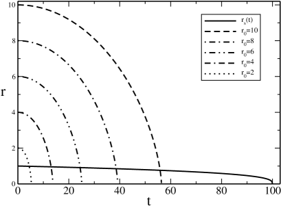
Figure 1: Trajectories of particles falling from different small multiples of $r_{s}(t=0)$ towards an evaporating black hole as modeled by the metric (31).

Note that by this choice of units, we are effectively considering black holes with a very low initial mass $M_{0}$. Indeed, it is possible to express the ratio between the characteristic times $\tau_{C}$, evaluated with the initial ($t=0$) Schwarzschild radius $r_{s0}$, and $t_{0}$ as

$$\frac{\tau_{C}}{t_{0}}=\frac{1}{5120}\left(\frac{r_{0}}{r_{s0}}\right)^{3/2}\left(\frac{m_{P}}{M_{0}}\right)^{2}\>,$$ (46)

where $m_{P}=\sqrt{\frac{\hbar c}{G}}=2.176\times 10^{-8}\>$kg is the Planck mass. To get this ratio close to one with $r_{0}/r_{s0}\approx 300$ (which roughly cancels the denominator 5120), we must have $M_{0}\approx m_{P}$. Let us assume $r_{0}=1\>\text{au}$ and check what mass $M_{0}$ is needed to obtain ${\tau_{C}}/{t_{0}}\approx 1$. It is useful to introduce $\tilde{m}_{0}\equiv c^{2}r_{0}/2G$ and to solve for $M_{0}/m_{P}$, which gives

$$\frac{M_{0}}{m_{P}}=\left(\frac{t_{0}}{\tau_{C}}\right)^{2/7}\frac{1}{5120^{2/7}}\left(\frac{\tilde{m}_{0}}{m_{P}}\right)^{3/7}\>,$$ (47)

providing a mass of $M_{0}=7.06\times 10^{10}\>$kg (that corresponds to the pretty small initial Schwarzschild radius $r_{s0}=1,05\times 10^{-16}\>$m) and a lifetime of $t_{0}\approx\tau_{C}\approx 9.38\times 10^{8}\>$a. Clearly, in scenarios of this kind (with a free-fall time of $10^{8}\>$a for just one astronomical unit) other masses that are present might affect the falling particle much stronger than the black hole (if we make the distance larger to reach an initially more massive black hole near the end of its life time, even distant stars will have to be taken into account as trajectory-perturbing factors). Therefore, in most real-life situations, we will have $\tau_{C}\ll t_{0}$. However, the only qualitative difference between this case and $\tau_{C}\lesssim t_{0}$ is that in the former case the curve describing $r_{s}(t)$ will be a straight line parallel to the time axis, whereas in the latter we see it approaching $r_{s}=0$.

What the calculation demonstrates is that letting the mass of the evaporating black hole depend on a time variable that does not get singular at $r_{s}$ and is meaningful also inside the Schwarzschild radius leads to an infalling particle or observer being able to cross $r_{s}$ without any problem, just as in the case of an eternal black hole. There are good reasons to believe that this is the generic behavior for any model using non-singular time coordinates to describe evaporation. In particular, the enormous separation of time scales between typical decay times of black holes and typical times to fall in one, suggests that the case of an evaporating black hole is indistinguishable from that of an eternal one, as far as crossing the “horizon” is concerned, in the large majority of cases.

Let us now consider whether $r_{s}(t)$ is a horizon indeed. First, it is clear that an outgoing radial light ray will momentarily hover at $r=r_{s}(t)$ with zero coordinate speed, as Eq. (31) degenerates to $\mathrm{d}r(\mathrm{d}r+2c\mathrm{d}t)=0$ there, so the solutions for the local speed of light are $\mathrm{d}r/\mathrm{d}t=0$ (outgoing ray) and $\mathrm{d}r/\mathrm{d}t=-2c$ (ingoing ray). However, after that instant $r_{s}$ has decreased a little, so the outgoing ray should have a positive velocity. This is clearly true for $r=r_{s}$, hence such a ray will escape. If we start our light ray inside $r_{s}$, however, escape may not be possible anymore. The numerical solution of Eq. (42) for several different initial conditions is depicted together with $r_{s}(t)$ in Fig. 2. The result demonstrates unambiguously that there is a range of initial conditions extending inside $r_{s}$ for which light can escape. On the other hand, light rays starting too far inside $r_{s}(0)$ will still hit the singularity. This means that a – time-dependent – event horizon continues to exist, separating events from which there is no escape to future null infinity and events from which a null ray can escape. However, the radial coordinate of that horizon is smaller than $r_{s}(t)$.

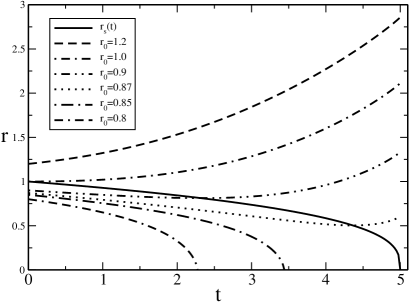
Figure 2: Light rays sent radially outward from different positions near the Schwarzschild radius or on it.

Finally, let us have a look at the case where an infalling particle approaches a black hole in a way that it would hit the position of the singularity only after the evaporation time $t_{0}$ (i.e., when the singularity is gone). From the preceding discussion, it should be clear given the vast disparity of time scales for falling and evaporation that such a phenomenon, while not impossible, requires quite some fine-tuning of the starting distance and time of the particle and the initial mass of the black hole. Figure 3 displays an example. Surprisingly, the particle starts getting repelled a short time before $r_{s}$ turns zero and ends up with positive radial velocity, i.e. moving away from the center of the mass distribution of the original black hole!

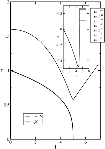
Figure 3: Particle falling radially onto a black hole that manages to evaporate before being hit. The inset gives the velocity as a function of time for a series of diminishing parameters $\varepsilon$ to demonstrate convergence.

While this is very counterintuitive at first sight, it is definitely predicted by the model. A look at Eq. (36) tells us that the deviation from Newton’s equation of motion, given by the second term on the right-hand side, is positive, i.e. repulsive, if $r_{s}$ decreases with increasing time – which is the case. Moreover, this term diverges as $r_{s}$ goes to zero. Since $r_{s,t}\propto(t_{0}-t)^{-2/3}$ and $1/\sqrt{r_{s}}\propto(t_{0}-t)^{-1/6}$, this divergence goes as $(t_{0}-t)^{-5/6}$ and is integrable. ($\dot{t}$ remains bounded.) Therefore, the velocity after $t=t_{0}$ will be finite. But it may be oriented away from the center, as the diverging repulsive term eventually exceeds the leading attractive term that goes to zero as $t\to t_{0}$. That the velocity is constant after complete evaporation of the black hole, is expected – the metric then is purely Minkowskian.

The unexpected behavior of the velocity of the infaller may be interpreted in two different ways. In the first, its counterintuitive aspects would be dismissed as a consequence of Newtonian thinking, making us believe that disappearance of mass from the center should only reduce gravitational attraction but not turn it into repulsion. In the Einstein approach, the disappearance of mass changes spacetime, i.e., it affects distances and time intervals. The same radial coordinate corresponds to a smaller proper distance to the center in the absence than in the presence of mass. If we assume that the proper distance as a physical measure of remoteness is continuous as central mass gets lost, this would suggest that the radial coordinate must increase in order to avoid a change of proper distance. This would result in an effective repulsion in terms of $r$.

The second way to interpret the repulsion would be to acknowledge that this is just a toy model, in which mass does not disappear via a well-defined physical process but rather by decree, so to speak. And while the mass function of time may be realistic for times that are small with respect to $t_{0}$, because there Hawking radiation can be described perturbatively, it will probably not describe things faithfully near the point of complete evaporation, where a fully quantum mechanical treatment is called for. This would then suggest that a more realistic decay law would not allow for a divergent term in the equation of motion. Rather, it would seem likely that the temporal decay happens much more smoothly towards the end, a conclusion that has been reached in Ref. [hiscock81a, ] for different reasons.

V Conclusions

In this paper, it was shown that there is no a priori reason to believe that Hawking radiation will make a black hole evaporate from under an observer, before she can fall in. While the argument is based on a toy model, not treating the time-dependent metric to be expected in the presence of Hawking radiation consistently, it has the advantage of a time coordinate leading to a metric that (a) does not become singular at the Schwarzschild radius $r_{s}(t)$ and (b) reduces to the Minkowski metric at infinity. The Aste-Trautmann modelaste05 does not have the first advantage, models based on Vaidya metricshiscock81a do not exhibit the second. Therefore, the toy model presented has the benefits of being both well-behaved and easily interpretable. The time in which the mass function following from Hawking radiation is usually expressed far from the black hole may be made to coincide with the model global time.

As it turns out, in this model the Schwarzschild radius is as easily crossed by a particle for an evaporating black hole as for an eternal one, and the crossing happens in finite time. This behavior is qualitatively different from that of the Aste-Trautmann model, which uses as input a dependence of the mass function on the Schwarzschild time. Conceptual problems of such an approach have been exposed.

What may be learned more generally from the results presented here?

Evidently, the slowing-down of an observer falling towards the horizon of a static black hole may be largely considered an optical illusion. After all, local coordinate stationary observers will not perceive any slowing-down, whereas the perception of a distant observer is readily explained in terms of gravitational redshift. The divergence of the Schwarzschild time on approach to the horizon is explicable as the consequence of an unfortunate coordinate choice. It is not a fact of physics but rather one resulting from a convention. An appropriate coordinate transformation removes the divergence.

However, things take a different twist, when time-dependent metrics are constructed by a generalization of either the Schwarzschild time or a non-singular time coordinate. The ensuing metrics are no longer related by a coordinate transformation but lead to physically different models. It then seems likely that the use of a coordinate that becomes singular at the Schwarzschild radius may produce spurious results.

Since the two models are different, the fact that they oppose each other even in a qualitative statement – one predicts crossing of the Schwarzschild radius while the other has the infaller freeze at the apparent horizon until the black hole has evaporated – is not extremely surprising. Of course, at most one of the models can be qualitatively right when compared with physical reality.

Finally, I would like to return to the question posed in the introduction whether a backreaction of the Hawking radiation might prevent formation of an event horizon or apparent horizon in the first place. Clearly, nothing rigorous can be said on the basis of the calculations presented here, as they do not consider backreaction. Nevertheless, our result may shed some light on the different approaches taken.

At least some of the treatments answering the question in the affirmativegerlach76 ; mersini14 use a Schwarzschild-type time coordinate to describe the outer metric of a collapsing star. This coordinate becomes singular at an apparent horizon the moment it forms. It may then be difficult to separate a spurious coordinate effect from a true delay of horizon formation. On the other hand, the approaches answering the question in the negative parentani94 ; paranjape09 ; modak14 generally seem to use non-singular coordinates for the relevant calculations.

Obviously, results denying the formation of a black hole would be much more convincing, if they were entirely obtained using coordinates that remain regular across apparent horizons.shankaranarayanan02

References

- (1) A. Aste and D. Trautmann, “Radial fall of a test particle onto an evaporating black hole,” Canad. J. Phys. 83, 1001–1006 (2005)
- (2) T. Vachaspati, D. Stojkovic, and L. M. Krauss, “Observation of incipient black holes and the information loss problem,” Phys. Rev. D 76, 024005 (2007)
- (3) T. M. Davis and C. H. Lineweaver, “Expanding Confusion: common misconceptions of cosmological horizons and the superluminal expansion of the universe,” Publ. Astron. Soc. Australia 21, 97–109 (2004)
- (4) A light signal sent from outside the Hubble sphere may reach us, due the the continuing expansion of the latter so it may eventually catch up with an inward-running light front. Once that light is inside the Hubble sphere, it will reach its center, in principle.
- (5) U.H. Gerlach, “The mechanism of blackbody radiation from an incipient black hole,” Phys. Rev. D 14, 1479–1508 (1976)
- (6) L. Mersini-Houghton, “Backreaction of Hawking radiation on a gravitationally collapsing star I: Black holes?.” Phys. Lett. 738, 61–67 (2014)
- (7) P.-M. Ho, “The absence of horizon in black-hole formation,” Nuclear Physics B 909, 394–417 (2016)
- (8) R. Parentani and T. Piran, “The internal geometry of an evaporating black hole,” Phys. Rev. Lett. 73, 2805–2808 (1994)
- (9) A. Paranjape and T. Padmanabhan, “Radiation from collapsing shells, semiclassical backreaction, and black hole formation,” Phys. Rev. D 80, 044011 (2009)
- (10) S.K. Modak, “Backreaction due to quantum tunneling and modification to the black hole evaporation process,” Phys. Rev. D 90, 044016 (2014)
- (11) A. Einstein, “Zur Elektrodynamik bewegter Körper,” Ann. Phys. 322, 891–921 (1905), English translation in The Principle of Relativity (Methuen, 1923, reprinted by Dover Publications, New York, 1952), pp. 35 – 65, “On the electrodynamics of moving bodies”.
- (12) A. Einstein, Relativity: The Special and the General Theory, 15 ed. (Crown, New York, 1952)
- (13) This procedure makes the one-way speed of light equal to its round-trip velocity.
- (14) G. Rizzi, M. L. Ruggiero, and A. Serafini, “Synchronization gauges and the principles of special relativity,” Found. Phys. 34, 1835–1887 (2004)
- (15) K. Kassner, “Ways to resolve Selleri’s paradox,” Am. J. Phys. 80, 1061–1066 (2012)
- (16) M. B. Cranor, E. M. Heider, and R. H. Price, “A circular twin paradox,” Am. J. Phys. 68, 1016–1020 (1999)
- (17) To understand why, imagine that the arclength of a planar curve and a local normal coordinate are to be extended from a strip about the curve to the whole plane. If the curve is not straight, it will have osculating circles of finite radius. Clearly, is not possible to assign a unique set of coordinates to the center of such a circle. The normal coordinate at two different arclengths will point to that center, so it is not described by a single arclength coordinate. The situation gets worse for points even farther away from the curve considered.
- (18) Standard clocks are running at the rate of their proper time. The clocks of the Global Positioning System are nonstandard clocks similar to the ones showing Schwarzschild time, except that they run slow with respect to a local standard clock, in order to keep them synchronous with clocks on Earth, not at infinity.
- (19) C. W. Misner, K. S. Thorne, and J. A. Wheeler, Gravitation (W. H. Freeman, New York, 1973)
- (20) This rate is identical to that of a (standard) master clock at infinity.
- (21) Kruskal-Szekeres coordinates escape this conclusion by the fact that a coordinate stationary observer necessarily crosses the horizon.
- (22) R. Spivey, “Dispelling black hole pathologies through theory and observation,” Progr. Phys. 11, 321–329 (2015)
- (23) A. A. Grib and Yu V. Pavlov, “Is it possible to see the infinite future of the Universe when falling into a black hole?.” Physics - Uspekhi 52, 257–261 (2009)
-
(24)
See, for example,
https://en.wikipedia.org/wiki/Kruskal-Szekeres_coordinates. - (25) There is also an antihorizon in the diagram, having . It is the times between these limits and that are missing from the horizons.
- (26) P. Painlevé, “La mécanique classique et la théorie de la relativité,” C. R. Acad. Sci. (Paris) 173, 677–680 (1921)
- (27) A. Gullstrand, “Allgemeine Lösung des statischen Einkörperproblems in der Einsteinschen Gravitationstheorie,” Arkiv. Mat. Astron. Fys. 16, 1–15 (1922)
- (28) We will assume this from now on, i.e., we set .
- (29) This speed corresponds to the one an object falling from rest at infinity would have at .
- (30) The light could be guided on the shell inside glass fibers, because for Einstein synchronization to work, we do not need the vacuum speed of light. All that is necessary is that the speed of the signal along the forward and backward directions of the fiber is the same.
- (31) T. Opatrný and L Richterek, “Black hole heat engine,” Am. J. Phys. 80, 66–71 (2012)
- (32) W. A. Hiscock, “Models of evaporating black holes. I,” Phys. Rev. D 23, 2813–2822 (1981)
- (33) W. H. Press, B. P. Flannery, S. A. Teukolsky, and W. T. Vetterling, Numerical Recipes (Cambridge University Press, Cambridge, 1986)
- (34) The trajectory of radial fall into the sun may be considered the first half of a degenerate Kepler ellipse with eccentricity 1, so the focus is the endpoint of the trajectory. The semimajor then is , with the radius of Earth’s orbit, making the “period” of that orbit equal to of the period of the Earth. So the time of fall to the center is a.
- (35) https://en.wikipedia.org/wiki/Spaghettification
- (36) The true proper time for falling to the singularity is of course somewhat longer in the model, as decreases.
- (37) However, as long as there is a central singularity, such a statement can be made only for distances measured from a shell outside the center, because the proper distance to the latter is not defined.
- (38) In Ref. [\rev@citealpnumpeiming16], the absence of a horizon may be spurious due to the choice of a generalization of outgoing Eddington-Finkelstein coordinates for the time dependent metric instead of the ingoing ones used in Ref. [\rev@citealpnumhiscock81a].
- (39) S. Shankaranarayanan, T. Padmanabhan, and K. Srinivasan, “Hawking radiation in different coordinate settings: complex paths approach,” Class. Quant. Grav. 19, 2671–2687 (2002)