A Hermite WENO reconstruction for fourth order temporal accurate schemes based on the GRP solver for hyperbolic conservation laws

Abstract.

This paper develops a new fifth order accurate Hermite WENO (HWENO) reconstruction method for hyperbolic conservation schemes in the framework of the two-stage fourth order accurate temporal discretization in [J. Li and Z. Du, A two-stage fourth order time-accurate discretization Lax–Wendroff type flow solvers, I. Hyperbolic conservation laws, SIAM, J. Sci. Comput., 38 (2016), pp. A3046–A3069]. Instead of computing the first moment of the solution additionally in the conventional HWENO or DG approach, we can directly take the interface values, which are already available in the numerical flux construction using the generalized Riemann problem (GRP) solver, to approximate the first moment. The resulting scheme is fourth order temporal accurate by only invoking the HWENO reconstruction twice so that it becomes more compact. Numerical experiments show that such compactness makes significant impact on the resolution of nonlinear waves.

Key Words. Hyperbolic conservation laws, Two-stage fourth-order accurate scheme, Hermite WENO reconstruction, GRP solver.

1. Introduction

In the development of high order accurate schemes for hyperbolic conservation laws, two families of approaches play important roles: one belongs to the method of line that achieves the temporal accuracy using the Runge-Kutta strategy [7, 27, 13, 8, 25]; the other is the Lax-Wendroff type approach that adopts the Cauchy-Kowaleveski expansions to design temporal-spatial coupled schemes [10, 1, 3, 15, 20, 31, 18]. Either family of approaches have their own advantages and disadvantages. The former has the simplicity in their practical implementation thanks to exact or approximate Riemann solvers, but the multi-stage temporal iteration inevitably causes the enlargement of the size of stencils; the latter can avoid the multi-stage temporal iteration but have to repeatedly make the differentiation of governing equations in order to construct high order accurate numerical fluxes. A recent two-stage fourth order accurate temporal discretization based on the Lax-Wendroff type solvers [11, 17] makes a compromise between these two families of methods: It just takes a two-stage iteration for the fourth order accuracy by using second order accurate temporal-spatial coupled Lax-Wendroff flow solvers so half of reconstruction steps can be saved in comparison with the same accurate method and complicated successive differentiations of governing equations can be avoided, which could be further extended using the multi-derivative Runge-Kutta methods [17, 5, 33]. Moreover, we notice that the solution values on cell interfaces already available in the procedure of numerical flux construction, called interface values in the present paper, can be used for the reconstruction procedure, thanks to the Lax-Wendroff flow solvers, which motivates us for such a study.

We develop a new fifth order accurate Hermite WENO (HWENO) reconstruction in the framework of two-stage fourth order accurate temporal discretization [11]. The HWENO interpolation adopts two values: the average value of the solution and the corresponding averaged gradient value (the first moment), as usual. The novelty is that the gradient values are directly approximated using the interface values when the Lax-Wendroff type flow solvers are used [1, 3, 18, 32], which is different from the standard HWENO method in [21, 22, 14]. Technically, we can further adjust nonlinear weights during the HWENO reconstruction, just like the WENO-Z method [4] modifying the classical WENO-JS [8]. In doing so, the resulting scheme is much more compact and has several distinct features.

1. The scheme just uses half of the reconstruction steps, compared with the standard RK-WENO methods.

2. The interface values are already available in the computation of numerical fluxes and no extra efforts are made on the gradient approximation.

3. The interface values are approximated by using the GRP solver and thus they are strong solution values without taking account of possible discontinuities in trouble cells.

4. A single HWENO reconstruction is more compact than the standard WENO reconstruction [8], as shown in other HWENO schemes [21, 22, 14].

This paper is organized as follows. In Section 2, we quickly review the two-stage method based on the Lax-Wendroff flow solvers and the HWENO reconstruction methods. In Section 3, we show the gradient approximation over each computational cell by using interface values of solutions. In Section 4, several numerical examples are displayed for the performance of such a HWENO reconstruction, by comparing with the WENO reconstruction with the same numerical flux. A discussion is made in Section 5.

2. The two-stage fourth oder method and the Hermite WENO reconstruction

This section serves to present a quick review of the two-stage fourth order method based on the Lax-Wendroff type flow solvers in [11] and the HWENO reconstruction procedure, originally in [21]. Instead of independently computing the first moment (the gradient of solution) in [21], we will construct it together with the solution average using the generalized Riemann problem (GRP) solver, which will be described in Setion 3.

2.1. Review of the two-stage fourth-order scheme

The two-stage fourth-order finite volume schemes based on the GRP solver was developed in [11]. Certainly, we can also use Men’shov’s modified GRP solver [15, 16] and the ADER solver [31, 32]. Both the acoustic and nonlinear versions of the GRP solver are provided in [3].

In this subsection, we quickly review this method by taking one-dimensional hyperbolic conservation laws,

(2.1) $$\begin{array}[]{l}\displaystyle{\frac{\partial\mathbf{u}}{\partial t}}+\displaystyle{\frac{\partial\mathbf{f}(\mathbf{u})}{\partial x}}=0,\ \ \ x\in\mathbb{R},t>0,\\[8.53581pt] \mathbf{u}(x,0)=\mathbf{u}_{0}(x),\ \ \ \ x\in\mathbb{R},\end{array}$$

where $\mathbf{u}$ is a vector of conservative variables and $\mathbf{f}(\mathbf{u})$ is the associated flux function vector. Given the computational mesh $I_{j}=(x_{j-\frac{1}{2}},x_{j+\frac{1}{2}})$ with the size $h=x_{j+\frac{1}{2}}-x_{j-\frac{1}{2}}$ for every $j$, we write (2.1) in form of the balance law,

(2.2) $${\frac{d\bar{\mathbf{u}}_{j}(t)}{dt}}=\mathcal{L}_{j}(\mathbf{u}):=-\displaystyle{\frac{1}{h}}[\mathbf{f}(\mathbf{u}(x_{j+\frac{1}{2}},t))-\mathbf{f}(\mathbf{u}(x_{j-\frac{1}{2}},t))],\ \ \ \bar{\mathbf{u}}_{j}(t)=\displaystyle{\frac{1}{h}}\int_{I_{j}}\mathbf{u}(x,t)dx,$$

where $\mathbf{u}(x_{j+\frac{1}{2}},t)$ is described in terms of GRP solver [3]. Then the two-stage approach for (2.1) is summarized as follows.

1. With the cell averages $\bar{\mathbf{u}}^{n}_{j}$ and interface values $\hat{\mathbf{u}}^{n}_{j+\frac{1}{2}}$, reconstruct the data at $t^{n}$ as a piece-wise polynomial function $\mathbf{u}(x,t^{n})=\mathbf{u}^{n}(x)$ by the HWENO interpolation that will be described below, and compute the corresponding GRP value $(\mathbf{u}_{j+\frac{1}{2}}^{n},(\partial\mathbf{u}/\partial t)_{j+\frac{1}{2}}^{n})$.

2. Compute the intermediate cell averages $\bar{\mathbf{u}}^{n+\frac{1}{2}}(x)$ and the interface values $\hat{\mathbf{u}}^{n+\frac{1}{2}}_{j+\frac{1}{2}}$ at $t^{n+\frac{1}{2}}=t^{n}+\frac{k}{2}$ using the formulae,

   (2.3) $$\begin{array}[]{l}\bar{\mathbf{u}}_{j}^{n+\frac{1}{2}}=\bar{\mathbf{u}}_{j}^{n}-\displaystyle{\frac{k}{2h}}[\mathbf{f}_{j+\frac{1}{2}}^{*}-\mathbf{f}_{j-\frac{1}{2}}^{*}],\\[8.53581pt] \displaystyle\mathbf{f}_{j+\frac{1}{2}}^{*}=\mathbf{f}(\mathbf{u}_{j+\frac{1}{2}}^{n})+\displaystyle{\frac{k}{4}}\displaystyle{\frac{\partial\mathbf{f}}{\partial\mathbf{u}}}({\mathbf{u}}^{n}_{j+\frac{1}{2}})\Big{(}\displaystyle{\frac{\partial\mathbf{u}}{\partial t}}\Big{)}^{n}_{j+\frac{1}{2}},\\[8.53581pt] \displaystyle\hat{\mathbf{u}}^{n+\frac{1}{2}}_{j+\frac{1}{2}}=\mathbf{u}_{j+\frac{1}{2}}^{n}+\frac{k}{2}\Big{(}\displaystyle{\frac{\partial\mathbf{u}}{\partial t}}\Big{)}_{j+\frac{1}{2}}^{n}.\end{array}$$

   where $k$ is the time step size and $\displaystyle{\frac{\partial\mathbf{f}}{\partial\mathbf{u}}}$ is the Jacobian of $\mathbf{f}(\mathbf{u})$. At this intermediate stage, the HWENO interpolation is carried out once again with the values $(\bar{\mathbf{u}}^{n+\frac{1}{2}}_{j},\hat{\mathbf{u}}^{n+\frac{1}{2}}_{j+\frac{1}{2}})$, to construct a piecewise polynomial $\mathbf{u}^{n+\frac{1}{2}}(x)$ and find the GRP value $(\mathbf{u}_{j+\frac{1}{2}}^{n+\frac{1}{2}},(\partial\mathbf{u}/\partial t)_{j+\frac{1}{2}}^{n+\frac{1}{2}})$, as done in Step 1.

3. Advance the solution to the next time level $t^{n+1}=t^{n}+k$ by

   (2.4) $$\begin{array}[]{l}\bar{\mathbf{u}}^{n+1}_{j}=\bar{\mathbf{u}}_{j}^{n}-\displaystyle{\frac{k}{h}}[\mathbf{f}_{j+\frac{1}{2}}^{4th}-\mathbf{f}_{j-\frac{1}{2}}^{4th}],\\[8.53581pt] \displaystyle\mathbf{f}_{j+\frac{1}{2}}^{4th}=\mathbf{f}(\mathbf{u}_{j+\frac{1}{2}}^{n})+\displaystyle{\frac{k}{2}}\Big{[}\displaystyle{\frac{1}{3}}\Big{(}\displaystyle{\frac{\partial\mathbf{f}}{\partial t}}\Big{)}^{n}_{j+\frac{1}{2}}+\displaystyle{\frac{2}{3}}\Big{(}\displaystyle{\frac{\partial\mathbf{f}}{\partial t}}\Big{)}^{n+\frac{1}{2}}_{j+\frac{1}{2}}\Big{]},\\[8.53581pt] \displaystyle\hat{\mathbf{u}}_{j+\frac{1}{2}}^{n+1}=\mathbf{u}_{j+\frac{1}{2}}^{n}+k\Big{(}\displaystyle{\frac{\partial\mathbf{u}}{\partial t}}\Big{)}_{j+\frac{1}{2}}^{n+\frac{1}{2}},\end{array}$$

   where the notations are

   $$\Big{(}\displaystyle{\frac{\partial\mathbf{f}}{\partial t}}\Big{)}^{n}_{j+\frac{1}{2}}=\displaystyle{\frac{\partial\mathbf{f}}{\partial\mathbf{u}}}(\mathbf{u}^{n}_{j+\frac{1}{2}})\Big{(}\displaystyle{\frac{\partial\mathbf{u}}{\partial t}}\Big{)}^{n}_{j+\frac{1}{2}},\ \ \ \Big{(}\displaystyle{\frac{\partial\mathbf{f}}{\partial t}}\Big{)}^{n+\frac{1}{2}}_{j+\frac{1}{2}}=\displaystyle{\frac{\partial\mathbf{f}}{\partial\mathbf{u}}}(\mathbf{u}^{n+\frac{1}{2}}_{j+\frac{1}{2}})\Big{(}\displaystyle{\frac{\partial\mathbf{u}}{\partial t}}\Big{)}^{n+\frac{1}{2}}_{j+\frac{1}{2}}.$$

The same procedure can be applied for two-dimensional cases. The details can be referred to [11].

Remark 2.1.

For this two-stage fourth order temporal accuracy method, the HWENO reconstruction is invoked only twice instead of four times from $t^{n}$ to $t^{n+1}=t^{n}+k$. In addition to save the computational cost, the size of stencils is automatically decreased.

2.2. A Hermite WENO Interpolation

In the approximation to a given function, there are two types of typical polynomial interpolations: the Lagrangian interpolation and the Hermite interpolation [24]. The former only uses the grid point values of the function, while the latter uses both the function value and its derivative value at the same grid point. It turns out that the latter uses half of grid points to derive the the polynomial approximations of the same degree to the given function compared to the former interpolation. So it is significant to develop a HWENO reconstruction technology for high order accurate schemes of hyperbolic conservation laws, as done in [21], so that the resulting scheme becomes more compact even though the same flux function approximation is adopted.

Let’s summarize the HWENO reconstruction in [21] for hyperbolic conservation laws in the finite volume framework although almost the same approach can be applied in the discontinuous Galerkin (DG) framework too [14]. Given the average $\bar{\mathbf{u}}_{j}$ and the derivative $\Delta\mathbf{u}_{j}$ of the function over the cell $I_{j}$,

(2.5) $$\bar{\mathbf{u}}_{j}=\displaystyle{\frac{1}{h}}\int_{I_{j}}\mathbf{u}(x,t)dx,\ \ \ \ \Delta\mathbf{u}_{j}=\displaystyle{\frac{1}{h}}\int_{I_{j}}\displaystyle{\frac{\partial\mathbf{u}}{\partial x}}(x,t)dx,$$

we want to construct a polynomial $p(x)$ such that $\mathbf{u}_{j+\frac{1}{2},-}:=p(x_{j+\frac{1}{2}})$ approximates the left limiting value of $\mathbf{u}(\cdot,t)$ at $x=x_{j+\frac{1}{2}}$.

We choose three stencils

(2.6) $$S^{(-1)}=I_{j-1}\cup I_{j},\ \ S^{(0)}=I_{j-1}\cup I_{j}\cup I_{j+1},\ \ S^{(1)}=I_{j}\cup I_{j+1}.$$

On stencil $S^{(0)}$, $\bar{\mathbf{u}}_{j-1}$, $\bar{\mathbf{u}}_{j}$ and $\bar{\mathbf{u}}_{j+1}$ are used to construct a polynomial $p^{(0)}$ for the interpolation. Hence at $x_{j+\frac{1}{2}}$, we have

(2.7) $$\mathbf{u}^{(0)}_{j+\frac{1}{2},-}:=p^{(0)}(x_{j+\frac{1}{2}})=-\displaystyle{\frac{1}{6}}\bar{\mathbf{u}}_{j-1}+\displaystyle{\frac{5}{6}}\bar{\mathbf{u}}_{j}+\displaystyle{\frac{1}{3}}\bar{\mathbf{u}}_{j+1}.$$

Similarly, $p^{(-1)}$ and $p^{(1)}$ are constructed by using $\bar{\mathbf{u}}_{j}$, $\bar{\mathbf{u}}_{j-1}$, $\Delta\mathbf{u}_{j-1}$ on $S^{(-1)}$ and by using $\bar{\mathbf{u}}_{j}$, $\bar{\mathbf{u}}_{j+1}$, $\Delta\mathbf{u}_{j+1}$ on $S^{(1)}$, respectively,

(2.8) $$\begin{array}[]{l}\mathbf{u}^{(-1)}_{j+\frac{1}{2},-}:=p^{(-1)}(x_{j+\frac{1}{2}})=-\displaystyle{\frac{7}{6}}\bar{\mathbf{u}}_{j-1}+\displaystyle{\frac{13}{6}}\bar{\mathbf{u}}_{j}-\displaystyle{\frac{2h}{3}}\Delta\mathbf{u}_{j-1},\\[8.53581pt] \mathbf{u}^{(1)}_{j+\frac{1}{2},-}:=p^{(1)}(x_{j+\frac{1}{2}})=\displaystyle{\frac{1}{6}}\bar{\mathbf{u}}_{j}+\displaystyle{\frac{5}{6}}\bar{\mathbf{u}}_{j+1}-\displaystyle{\frac{h}{3}}\Delta\mathbf{u}_{j+1}.\end{array}$$

If the solution is smooth on the large stencil $I_{-1}\cup I_{0}\cup I_{1}$, we have

(2.9) $$\tilde{\mathbf{u}}_{j+\frac{1}{2},-}=\displaystyle{\frac{1}{120}}(-23\bar{\mathbf{u}}_{j-1}+76\bar{\mathbf{u}}_{j}+67\bar{\mathbf{u}}_{j+1}-9h\Delta\mathbf{u}_{j-1}-21h\Delta\mathbf{u}_{j+1}).$$

Thus the linear weights of the three stencils are

(2.10) $$\gamma^{(-1)}=\displaystyle{\frac{9}{80}},\ \ \gamma^{(0)}=\displaystyle{\frac{29}{80}},\ \ \gamma^{(1)}=\displaystyle{\frac{21}{40}},$$

which ensure

$$\tilde{\mathbf{u}}_{j+\frac{1}{2},-}=\displaystyle\sum_{r=-1}^{1}\gamma^{(r)}\mathbf{u}^{(r)}_{j+\frac{1}{2},-}.$$

The smoothness indicators are defined by

(2.11) $$\beta^{(r)}=\displaystyle\sum_{l=1}^{2}\int_{I_{j}}h^{2l-1}\left(\displaystyle{\frac{d^{l}}{dx^{l}}}p^{(r)}(x)\right)^{2}dx,\ \ r=-1,0,1,$$

in the same way as in the WENO reconstructions where $p^{(r)}(x)$ is the interpolation polynomial on stencil $S^{(r)}$. Their explicit expressions are

(2.12) $$\begin{array}[]{l}\beta^{(-1)}=(-2\bar{\mathbf{u}}_{j-1}+2\bar{\mathbf{u}}_{j}-h\Delta\mathbf{u}_{j-1})^{2}+\displaystyle{\frac{13}{3}}(-\bar{\mathbf{u}}_{j-1}+\bar{\mathbf{u}}_{j}-h\Delta\mathbf{u}_{j-1})^{2},\\[8.53581pt] \beta^{(0)}=\displaystyle{\frac{1}{4}}(-\bar{\mathbf{u}}_{j-1}+\bar{\mathbf{u}}_{j+1})^{2}+\displaystyle{\frac{13}{12}}(-\bar{\mathbf{u}}_{j-1}+2\bar{\mathbf{u}}_{j}-\bar{\mathbf{u}}_{j+1})^{2},\\[8.53581pt] \beta^{(1)}=(2\bar{\mathbf{u}}_{j+1}-2\bar{\mathbf{u}}_{j}-h\Delta\mathbf{u}_{j+1})^{2}+\displaystyle{\frac{13}{3}}(\bar{\mathbf{u}}_{j+1}-\bar{\mathbf{u}}_{j}-h\Delta\mathbf{u}_{j+1})^{2}.\end{array}$$

Then we compute the nonlinear weights in the same way as the WENO-Z method does

(2.13) $$\omega^{\text{z}}_{r}=\displaystyle{\frac{\alpha^{\text{z}}_{r}}{\sum_{l}\alpha_{l}}},\ \ \ \alpha^{\text{z}}_{r}=\gamma^{(r)}(1+\displaystyle{\frac{\tau^{\text{z}}}{\beta^{(r)}+\varepsilon}}),\ \ \ r=-1,0,1,$$

where $\varepsilon$ is a small parameter in order to avoid a zero denominator and $\tau^{\text{z}}=|\beta^{(1)}-\beta^{(-1)}|$. Finally we have

(2.14) $$\mathbf{u}_{j+\frac{1}{2},-}=\displaystyle\sum_{r=-1}^{1}\omega^{\text{z}}_{r}\mathbf{u}^{(r)}_{j+\frac{1}{2},-}.$$

The right interface value $\mathbf{u}_{j-\frac{1}{2},+}$ can be reconstructed in a similar way by mirroring the above procedure with respect to $x_{j}=\displaystyle{\frac{1}{2}}(x_{j-\frac{1}{2}}+x_{j+\frac{1}{2}})$.

Since the GRP solver has to use the spatial derivative $(\partial\mathbf{u}/\partial x)_{j+\frac{1}{2},\pm}$, we approximate them using the interpolation,

(2.15) $$\Big{(}\displaystyle{\frac{\partial\mathbf{u}}{\partial x}}\Big{)}_{j+\frac{1}{2},\pm}:=\displaystyle{\frac{1}{12h}}\left(\bar{\mathbf{u}}_{j-1}-15\bar{\mathbf{u}}_{j}+15\bar{\mathbf{u}}_{j+1}-\bar{\mathbf{u}}_{j+2}\right).$$

The practical simulations later on indicate that the WENO-type stencil selection procedure in (2.15) can be avoided and the similar observation can be found in [23, 9].

In [21], the approaches for deriving $\Delta\mathbf{u}_{j}$ were proposed both for the DG method and the finite volume method. In the current study, we use the GRP solver to obtain it, without extra manipulation of governing equations in Section 3.

3. Construction of gradients based on the GRP solver

It is already presented in the original GRP scheme [2, 3] using interface values for the gradient reconstruction. Now we want to apply the idea for the HWENO reconstruction procedure.

3.1. One-dimensional case

First we discuss the one-dimensional case. Over the computational cell $I_{j}$, we regard $\Delta\mathbf{u}_{j}$ as the average of the corresponding spatial derivative,

(3.1) $$\Delta\mathbf{u}_{j}=\displaystyle{\frac{1}{h}}\int_{I_{j}}\displaystyle{\frac{\partial\mathbf{u}}{\partial x}}(x,t)dx=\displaystyle{\frac{1}{h}}\left(\mathbf{u}(x_{j+\frac{1}{2}},t)-\mathbf{u}(x_{j-\frac{1}{2}},t)\right),$$

where the second equality is the Newton-Leibniz formula. Assume that the GRP values $(\mathbf{u}_{j+\frac{1}{2}}^{n},(\partial\mathbf{u}/\partial t)_{j+\frac{1}{2}}^{n})$ and $(\mathbf{u}_{j+\frac{1}{2}}^{n+\frac{1}{2}},(\partial\mathbf{u}/\partial t)_{j+\frac{1}{2}}^{n+\frac{1}{2}})$ are available around each grid point $x=x_{j+\frac{1}{2}}$. Then we obtain the interface values for any time $t\in(t_{n},t_{n+1})$. In particular, we have

(3.2) $$\hat{\mathbf{u}}^{n+\frac{1}{2}}_{j+\frac{1}{2}}=\mathbf{u}_{j+\frac{1}{2}}^{n}+\frac{k}{2}\Big{(}\displaystyle{\frac{\partial\mathbf{u}}{\partial t}}\Big{)}_{j+\frac{1}{2}}^{n},\ \ \ \hat{\mathbf{u}}^{n+1}_{j+\frac{1}{2}}=\mathbf{u}_{j+\frac{1}{2}}^{n}+k\Big{(}\displaystyle{\frac{\partial\mathbf{u}}{\partial t}}\Big{)}_{j+\frac{1}{2}}^{n+\frac{1}{2}}.$$

It turns out that

(3.3) $$\Delta\mathbf{u}^{n+\frac{1}{2}}_{j}=\displaystyle{\frac{1}{h}}\left(\hat{\mathbf{u}}^{n+\frac{1}{2}}_{j+\frac{1}{2}}-\hat{\mathbf{u}}^{n+\frac{1}{2}}_{j-\frac{1}{2}}\right),\ \ \ \Delta\mathbf{u}^{n+1}_{j}=\displaystyle{\frac{1}{h}}\left(\hat{\mathbf{u}}^{n+1}_{j+\frac{1}{2}}-\hat{\mathbf{u}}^{n+1}_{j-\frac{1}{2}}\right).$$

These values, together with the solution averages $\bar{\mathbf{u}}_{j}^{n+\frac{1}{2}}$ and $\bar{\mathbf{u}}_{j}^{n+1}$, are used in the HWENO reconstruction at the intermediate stage $t^{n+\frac{1}{2}}$ and the final time stage $t^{n+1}$, respectively.

Now we analyze that such a construction has the desired accuracy. This is not obvious because the interface values $\hat{\mathbf{u}}_{j+\frac{1}{2}}^{n+\frac{1}{2}}$ and $\hat{\mathbf{u}}_{j+\frac{1}{2}}^{n+1}$ bear truncation errors of lower orders compared with those of the cell averages. That is, $\hat{\mathbf{u}}_{j+\frac{1}{2}}^{n+\frac{1}{2}}$ is first order accurate since it is evaluated by the forward Euler evolution in (2.3) and $\hat{\mathbf{u}}_{j+\frac{1}{2}}^{n+1}$ is second order accurate with the mid-point rule in (2.4). One might wonder whether the reconstruction can still achieve the desired order of accuracy.

Recall that the fourth-order accurate numerical flux is defined as

(3.4) $$\begin{array}[]{rl}k\mathbf{f}_{j+\frac{1}{2}}^{4th}&=k\mathbf{f}(\mathbf{u}_{j+\frac{1}{2}}^{n})+\displaystyle{\frac{k^{2}}{2}}\Big{[}\displaystyle{\frac{1}{3}}\displaystyle{\frac{\partial\mathbf{f}}{\partial\mathbf{u}}}(\mathbf{u}^{n}_{j+\frac{1}{2}})\Big{(}\displaystyle{\frac{\partial\mathbf{u}}{\partial t}}\Big{)}^{n}_{j+\frac{1}{2}}+\displaystyle{\frac{2}{3}}\displaystyle{\frac{\partial\mathbf{f}}{\partial\mathbf{u}}}(\mathbf{u}^{n+\frac{1}{2}}_{j+\frac{1}{2}})\Big{(}\displaystyle{\frac{\partial\mathbf{u}}{\partial t}}\Big{)}^{n+\frac{1}{2}}_{j+\frac{1}{2}}\Big{]}\\[8.53581pt] &=k\mathbf{f}(\mathbf{u}_{j+\frac{1}{2}}^{n})+\displaystyle{\frac{k^{2}}{2}}\Big{[}-\displaystyle{\frac{1}{3}}\Big{(}\displaystyle{\frac{\partial\mathbf{f}}{\partial\mathbf{u}}}(\mathbf{u}^{n}_{j+\frac{1}{2}})\Big{)}^{2}\Big{(}\displaystyle{\frac{\partial\mathbf{u}}{\partial x}}\Big{)}^{n}_{j+\frac{1}{2}}-\displaystyle{\frac{2}{3}}\Big{(}\displaystyle{\frac{\partial\mathbf{f}}{\partial\mathbf{u}}}(\mathbf{u}^{n+\frac{1}{2}}_{j+\frac{1}{2}})\Big{)}^{2}\Big{(}\displaystyle{\frac{\partial\mathbf{u}}{\partial x}}\Big{)}^{n+\frac{1}{2}}_{j+\frac{1}{2}}\Big{]}\\[8.53581pt] &=\displaystyle\int_{t^{n}}^{t^{n+1}}\mathbf{f}(\mathbf{u}(x_{j+\frac{1}{2}},t))dt+\mathcal{O}(k^{5}),\end{array}$$

where $(\mathbf{u}^{n}_{j+\frac{1}{2}},(\partial\mathbf{u}/\partial x)^{n}_{j+\frac{1}{2}})$ and $(\mathbf{u}^{n+\frac{1}{2}}_{j+\frac{1}{2}},(\partial\mathbf{u}/\partial x)^{n+\frac{1}{2}}_{j+\frac{1}{2}})$ are the GRP values. This shows that the tolerance for the errors of $\mathbf{u}_{j+\frac{1}{2}}^{n}$ is $\mathcal{O}(k^{4})$. And the tolerance for the errors of $\mathbf{u}_{j+\frac{1}{2}}^{n+\frac{1}{2}}$, $(\partial\mathbf{u}/\partial x)_{j+\frac{1}{2}}^{n}$ and $(\partial\mathbf{u}/\partial x)_{j+\frac{1}{2}}^{n+\frac{1}{2}}$ is $\mathcal{O}(k^{3})$.

The Taylor expansion for $\hat{\mathbf{u}}_{j+\frac{1}{2}}^{n+\frac{1}{2}}$ gives

(3.5) $$\hat{\mathbf{u}}^{n+\frac{1}{2}}_{j+\frac{1}{2}}=\mathbf{u}_{j+\frac{1}{2}}^{n}+\displaystyle{\frac{k}{2}}\left(\displaystyle{\frac{\partial\mathbf{u}}{\partial t}}\right)_{j+\frac{1}{2}}^{n}=\mathbf{u}(x_{j+\frac{1}{2}},t^{n+\frac{1}{2}})-\displaystyle{\frac{k^{2}}{8}}\left.\displaystyle{\frac{\partial^{2}\mathbf{u}}{\partial t^{2}}}\right|_{j+\frac{1}{2}}^{n}+\mathcal{O}(k^{3}).$$

By the definition of $\Delta\mathbf{u}_{j}^{n+\frac{1}{2}}$ in (3.3), we have

(3.6) $$\begin{array}[]{l}h\Delta\mathbf{u}^{n+\frac{1}{2}}_{j}=\hat{\mathbf{u}}^{n+\frac{1}{2}}_{j+\frac{1}{2}}-\hat{\mathbf{u}}^{n+\frac{1}{2}}_{j-\frac{1}{2}}\\ \ \ \ \ \ \ \ \ \ \ \ =\mathbf{u}(x_{j+\frac{1}{2}},t^{n+\frac{1}{2}})-\mathbf{u}(x_{j-\frac{1}{2}},t^{n+\frac{1}{2}})-\displaystyle{\frac{k^{2}}{8}}\left(\left.\displaystyle{\frac{\partial^{2}\mathbf{u}}{\partial t^{2}}}\right|_{j+\frac{1}{2}}^{n}-\left.\displaystyle{\frac{\partial^{2}\mathbf{u}}{\partial t^{2}}}\right|_{j-\frac{1}{2}}^{n}\right)+\mathcal{O}(k^{4})\\ \ \ \ \ \ \ \ \ \ \ \ =\displaystyle\int_{I_{j}}\displaystyle{\frac{\partial\mathbf{u}}{\partial x}}(x,t^{n+\frac{1}{2}})dx-\displaystyle{\frac{k^{2}h}{8}}\left.\displaystyle{\frac{\partial^{3}\mathbf{u}}{\partial t^{2}\partial x}}\right|_{j-\frac{1}{2}}^{n}+\mathcal{O}(k^{4}).\end{array}$$

Since $h$ and $k$ are proportional thanks to the CFL condition, $h\Delta\mathbf{u}^{n+\frac{1}{2}}_{j}$ bears the truncation error $\mathcal{O}(k^{3})$. Therefore $\mathbf{u}_{j+\frac{1}{2},\pm}^{n+\frac{1}{2}}$ is approximated with error $\mathcal{O}(k^{3})$ in (2.9). Finally, since the Riemann solution $\mathbf{u}_{j+\frac{1}{2}}^{n+\frac{1}{2}}$ is calculated from the data $\mathbf{u}_{j+\frac{1}{2},\pm}^{n+\frac{1}{2}}$, we conclude that it has the error $\mathcal{O}(k^{3})$.

At the time step $t^{n+1}$, it is obvious that the cell average $\bar{\mathbf{u}}_{j}^{n+1}$ has the error $\mathcal{O}(k^{5})$, as shown in [11]. As for the cell boundary values $\hat{\mathbf{u}}_{j+\frac{1}{2}}^{n+1}$, they are second order accurate thanks to the mid-point rule,

(3.7) $$\hat{\mathbf{u}}_{j+\frac{1}{2}}^{n+1}=\mathbf{u}_{j+\frac{1}{2}}^{n}+k\left(\displaystyle{\frac{\partial\mathbf{u}}{\partial t}}\right)_{j+\frac{1}{2}}^{n+\frac{1}{2}}=\mathbf{u}(x_{j+\frac{1}{2}},t^{n+1})-\displaystyle{\frac{k^{3}}{24}}\left.\displaystyle{\frac{\partial^{3}\mathbf{u}}{\partial t^{3}}}\right|_{j+\frac{1}{2}}^{n}+\mathcal{O}(k^{4}),$$

which further gives

(3.8) $$\begin{array}[]{l}h\Delta\mathbf{u}^{n+1}_{j}=\displaystyle\int_{I_{j}}\displaystyle{\frac{\partial\mathbf{u}}{\partial x}}(x,t^{n+1})dx-\displaystyle{\frac{k^{3}h}{24}}\left.\displaystyle{\frac{\partial^{4}\mathbf{u}}{\partial t^{3}\partial x}}\right|_{j-\frac{1}{2}}^{n}+\mathcal{O}(k^{5}).\end{array}$$

With the same arguement, we can show that $h\Delta\mathbf{u}^{n+1}_{j}$ bears an error $\mathcal{O}(k^{4})$. Therefore the Riemann solution $\mathbf{u}_{j+\frac{1}{2}}^{n+1}$ bears $\mathcal{O}(k^{4})$.

With (2.15), we can show that $(\partial\mathbf{u}/\partial x)_{j+\frac{1}{2},\pm}^{n+\frac{1}{2}}$ and $(\partial\mathbf{u}/\partial x)_{j+\frac{1}{2},\pm}^{n}$ bear errors of orders $\mathcal{O}(k^{3})$ and $\mathcal{O}(k^{4})$, respectively, which meet the above requirement.

3.2. Two-dimensional cases

In this subsection, we supress the dependence of $\mathbf{u}$ on the variable $t$ to simplify the presentation. The gradient construction for two-dimensional cases can be treated similarly. Let $\Omega_{J}$ be a computational cell, with the boundary $L_{J\ell}$, $\ell=1,\cdots,K$. Then we use the Gauss theorem to have

(3.9) $$\nabla\mathbf{u}_{J}:=\displaystyle{\frac{1}{|\Omega_{J}|}}\int_{\Omega_{J}}\nabla\mathbf{u}(x,y)dxdy=\displaystyle{\frac{1}{|\Omega_{J}|}}\sum_{\ell=1}^{K}\int_{L_{J_{\ell}}}\mathbf{u}\mathbf{n}_{J_{\ell}}dL,$$

where $\mathbf{n}_{J_{\ell}}$ is the unit outer normal of $\Omega_{J}$ on $L_{J_{\ell}}$. Therefore, once we know the interface values on $L_{J_{\ell}}$, we can approximate the gradient $\nabla\mathbf{u}_{J}$ as

(3.10) $$\nabla\mathbf{u}_{J}\approx\displaystyle{\frac{1}{|\Omega_{J}|}}\sum_{\ell=1}^{K}\sum_{m}^{M}\omega_{J_{\ell m}}\hat{\mathbf{u}}_{J_{\ell m}}\mathbf{n}_{J_{\ell m}}|L_{J_{\ell}}|=:\left[\begin{array}[]{c}\Delta_{x}\mathbf{u}_{J}\\ \Delta_{y}\mathbf{u}_{J}\end{array}\right],$$

where $\hat{\mathbf{u}}_{J_{\ell m}}$ is the interface value at the Gauss point $\mathbf{x}_{J_{\ell m}}$ on the interface $L_{J_{\ell}}$ and $\omega_{J_{\ell m}}$ is the corresponding Gauss weight.

Specified to the uniformly rectangular meshes $\Omega_{J}=\Omega_{ij}=[x_{i-\frac{1}{2}},x_{i+\frac{1}{2}}]\times[y_{j-\frac{1}{2}},y_{j+\frac{1}{2}}]$ for which $h_{x}=x_{i+\frac{1}{2}}-x_{i-\frac{1}{2}}$ and $h_{y}=y_{i+\frac{1}{2}}-y_{i-\frac{1}{2}}$, there are two Gaussian quadrature points on each boundary of $\Omega_{ij}$ to achieve the fifth order accuracy in space. For example we have $(x_{i+\frac{1}{2}},y_{j_{1}})$ and $(x_{i+\frac{1}{2}},y_{j_{2}})$ on $x=x_{i+\frac{1}{2}}$ for $y\in[y_{j-\frac{1}{2}},y_{j+\frac{1}{2}}]$, with $y_{j_{1}}=\frac{1+\sqrt{3}}{2}y_{j-\frac{1}{2}}+\frac{1-\sqrt{3}}{2}y_{j+\frac{1}{2}}$ and $y_{j_{2}}=\frac{1-\sqrt{3}}{2}y_{j-\frac{1}{2}}+\frac{1+\sqrt{3}}{2}y_{j+\frac{1}{2}}$. The corresponding weights are taken as $\omega_{1}=\omega_{2}=\frac{1}{2}$. As for the outer normals, we have

(3.11) $$\mathbf{n}_{i\pm\frac{1}{2},j_{m}}=\left[\begin{array}[]{c}\pm 1\\ 0\end{array}\right],\ \ \ \mathbf{n}_{i_{m},j\pm\frac{1}{2}}=\left[\begin{array}[]{c}0\\ \pm 1\end{array}\right],\ \ \ m=1,2.$$

It turns out that, by combining (3.10) and (3.11), the gradient $\nabla\mathbf{u}_{ij}$ is approximated as

(3.12) $$\begin{array}[]{l}\Delta_{x}\mathbf{u}_{ij}=\displaystyle{\frac{1}{h_{x}}}\left[\displaystyle{\frac{1}{2}}(\hat{\mathbf{u}}_{i+\frac{1}{2},j_{1}}+\hat{\mathbf{u}}_{i+\frac{1}{2},j_{2}})-\displaystyle{\frac{1}{2}}(\hat{\mathbf{u}}_{i-\frac{1}{2},j_{1}}+\hat{\mathbf{u}}_{i-\frac{1}{2},j_{2}})\right],\\[8.53581pt] \Delta_{y}\mathbf{u}_{ij}=\displaystyle{\frac{1}{h_{y}}}\left[\displaystyle{\frac{1}{2}}(\hat{\mathbf{u}}_{i_{1},j+\frac{1}{2}}+\hat{\mathbf{u}}_{i_{2},j+\frac{1}{2}})-\displaystyle{\frac{1}{2}}(\hat{\mathbf{u}}_{i_{1},j-\frac{1}{2}}+\hat{\mathbf{u}}_{i_{2},j-\frac{1}{2}})\right],\end{array}$$

which are the componentwise expressions of (3.10) over the rectangular grids.

Now we need the limiting values of the solution $\mathbf{u}$ and its derivatives at each Gaussian quadrature point on the cell boundaries, i.e., $\mathbf{u}_{i_{m},(j+\frac{1}{2},\pm)}$, $(\frac{\partial\mathbf{u}}{\partial y})_{i_{m},(j+\frac{1}{2},\pm)}$, $(\frac{\partial\mathbf{u}}{\partial x})_{i_{m},(j+\frac{1}{2},\pm)}$, $\mathbf{u}_{(i+\frac{1}{2},\pm),j_{m}}$, $(\frac{\partial\mathbf{u}}{\partial x})_{(i+\frac{1}{2},\pm),j_{m}}$ and $(\frac{\partial\mathbf{u}}{\partial y})_{(i+\frac{1}{2},\pm),j_{m}}$ for $m=1,2$. We adopt the dimension-by-dimension strategy conventionally used over rectangular grids [28] to interpolate them.

With $(\bar{\mathbf{u}}_{ij},\Delta_{x}\mathbf{u}_{ij})$, we implement the HWENO reconstruction on $\mathbf{u}$ in the $x$-direction to obtain the line average of $\mathbf{u}$ over $y\in[{y_{j-\frac{1}{2}}},{y_{j+\frac{1}{2}}}]$ at $x_{i_{1}}$ and $x_{i_{2}}$, i.e.,

(3.13) $$\overline{\mathbf{u}(x_{i_{m}},\cdot)}_{j}:=\displaystyle{\frac{1}{h_{y}}}\int_{y_{j-\frac{1}{2}}}^{y_{j+\frac{1}{2}}}\mathbf{u}(x_{i_{m}},y)dy,\ \ m=1,2.$$

Different from the procedure for one-dimensional case in Subsection 2.2, we interpolate at the Gaussian quadrature points $x_{i_{1}}$ and $x_{i_{2}}$ instead of the boundaries. Thus the formulae (2.7) to (2.10) are modified correspondingly. Furthermore, we have

(3.14) $$\Delta\mathbf{u}(x_{i_{m}},\cdot)_{j}=\displaystyle{\frac{1}{h_{y}}}(\hat{\mathbf{u}}_{i_{m},j+\frac{1}{2}}-\hat{\mathbf{u}}_{i_{m},j-\frac{1}{2}})\ \ m=1,2.$$

Finally, we implement the HWENO reconstruction for $\mathbf{u}(x_{i_{m}},\cdot)$ with $(\overline{\mathbf{u}(x_{i_{m}},\cdot)}_{j},(\Delta_{y}\mathbf{u}(x_{i_{m}},\cdot))_{j})$ defined in (3.13) and (3.14) to obtain $\mathbf{u}(x_{i_{m}},y_{j+\frac{1}{2},\pm})$ and $\frac{\partial\mathbf{u}}{\partial y}(x_{i_{m}},y_{j+\frac{1}{2},\pm})$, which are just $\mathbf{u}_{i_{m},(j+\frac{1}{2},\pm)}$ and $(\frac{\partial\mathbf{u}}{\partial y})_{i_{m},(j+\frac{1}{2},\pm)}$.

As for the tangential derivatives $(\frac{\partial\mathbf{u}}{\partial x})_{i_{m},(j+\frac{1}{2},\pm)}$, implement the HWENO reconstruction on $\mathbf{u}$ with $(\bar{\mathbf{u}}_{ij},\Delta_{y}\mathbf{u}_{ij})$ in the $y$-direction to obtain the line average of $\mathbf{u}$ over $x\in[{x_{i-\frac{1}{2}}},{x_{i+\frac{1}{2}}}]$ at $y_{j+\frac{1}{2},\pm}$, i.e.,

$$\overline{\mathbf{u}(\cdot,y_{j+\frac{1}{2},\pm})}_{i}:=\displaystyle\frac{1}{h_{x}}\int_{i-\frac{1}{2}}^{i+\frac{1}{2}}\mathbf{u}(x,y_{j+\frac{1}{2},\pm})dx.$$

With $\overline{\mathbf{u}(\cdot,y_{j+\frac{1}{2},\pm})}_{i}$ already obtained above, we interpolate the derivatives of $\mathbf{u}(\cdot,y_{j+\frac{1}{2},\pm})$ at $x_{i_{1}}$ as

(3.15) $$\begin{array}[]{rl}&\displaystyle{\frac{\partial\mathbf{u}}{\partial x}}(x_{i_{1}},y_{j+\frac{1}{2},\pm})\\[8.53581pt] =&\displaystyle{\frac{1}{108h_{x}}}\left[(9+2\sqrt{3})\overline{\mathbf{u}(\cdot,y_{j+\frac{1}{2},\pm})}_{i-2}-(72+26\sqrt{3})\overline{\mathbf{u}(\cdot,y_{j+\frac{1}{2},\pm})}_{i-1}\right.\\[8.53581pt] &\left.+48\sqrt{3}~{}\overline{\mathbf{u}(\cdot,y_{j+\frac{1}{2},\pm})}_{i}+(72-26\sqrt{3})\overline{\mathbf{u}(\cdot,y_{j+\frac{1}{2},\pm})}_{i+1}-(9-2\sqrt{3})\overline{\mathbf{u}(\cdot,y_{j+\frac{1}{2},\pm})}_{i+2}\right],\end{array}$$

which is just $(\frac{\partial\mathbf{u}}{\partial x})_{i_{1},(j+\frac{1}{2},\pm)}$, the tangential derivative of $\mathbf{u}$ at the Gaussian quadrature point $(x_{i_{1}},y_{j+\frac{1}{2},\pm})$. We can obtain $(\frac{\partial\mathbf{u}}{\partial x})_{i_{2},(j+\frac{1}{2},\pm)}$ by simply mirroring (3.15) with respect to $(x_{i},y_{j+\frac{1}{2},\pm})$.

Similar interpolations are made for $\mathbf{u}_{(i+\frac{1}{2},\pm),j_{m}}$, $(\frac{\partial\mathbf{u}}{\partial x})_{(i+\frac{1}{2},\pm),j_{m}}$ and $(\frac{\partial\mathbf{u}}{\partial y})_{(i+\frac{1}{2},\pm),j_{m}}$ for $m=1,2$. The details are omitted.

For system cases, the characteristic decomposition in [28] is adopted in the current study. All the reconstruction procedures described above are applied for the characteristic variables. The details are omitted here.

4. Numerical Examples

In this section, we provide several examples for one- and two-dimensional compressible Euler equations to verify the expected performance of this approach. The Euler equations can be found in any CFD books and we do not write out them here. Each example will be computed with the HWENO interpolation and the WENO interpolation in the same framework of two-stage fourth-order time discretization based the GRP solver [11]. Both the HWENO and the WENO reconstruction use the nonlinear weights in formulae (2.13). The resulting schemes are denoted as GRP4-HWENO5 and GRP4-WENO5, respectively. We emphasize again that the only difference is the data reconstruction. The CFL number $0.6$ is used for all the computations except in the first example.

Example 1. Smooth initial value problem. We check the numerical results for a one-dimensional smooth initial value problem of the Euler equations with the initial data

(4.1) $$\rho(x,0)=1+0.2\text{sin}(\pi x),\ \ \ v(x,0)=1,\ \ p(x,0)=1,$$

to verify the numerical accuracy of the present approach where $\rho$ is the density, $v$ is the velocity, $p$ is the pressure and $\mathbf{u}=[\rho,v,p]^{\top}$. The periodic boundary conditions are used. The exact solution at time $t$ is just a shift of the initial condition, i.e.

(4.2) $$\mathbf{u}(x,t)=\mathbf{u}(x-t,0).$$

Here we set the CFL number to be $0.1$ to show the numerical order of the spatial reconstructions. The errors shown in Table 1 are those of the cell averages of the density $\rho$ at time $t=10$.

Both reconstruction approaches achieve the designed numerical order while the errors of the scheme GRP4-HWENO5 is smaller than those of GRP4-WNEO5. And we can see that the the CPU time cost by both schemes are almost the same which verifies our claim that no additional efforts are made to obtain the first moment of the solution.

Table 1. The $L_{1}$, $L_{\infty}$ errors of the density and numerical orders for the smooth initial value problem in Example 1. The results are shown at time $t=10$.

$m$	GRP4-WENO5					GRP4-HWENO5
	CPU time (s)	$L_{1}$ error	Order	$L_{\infty}$ error	Order	CPU time (s)	$L_{1}$ error	Order	$L_{\infty}$ error	Order
40	0.31	6.25e-6	4.98	9.83e-6	4.99	0.41	1.50e-6	4.99	2.36e-6	5.02
80	1.25	1.96e-7	4.99	3.08e-7	5.00	1.46	4.69e-8	5.00	7.37e-8	5.00
160	5.14	6.13e-9	5.00	9.64e-9	5.00	4.95	1.47e-9	5.00	2.30e-9	5.00
320	19.77	1.92e-10	5.00	3.01e-10	5.00	19.61	4.59e-11	5.00	7.21e-11	5.00
640	122.38	5.99e-12	5.00	9.47e-12	4.99	117.23	1.43e-12	5.00	2.36e-12	4.93

Example 2. The Titarev-Toro problem. This example was proposed in [30] as an extension of the Shu-Osher problem [26]. The initial data is taken as

(4.3) $$(\rho,v,p)(x,0)=\left\{\begin{array}[]{ll}(1.515695,0.523346,1.805),&\mbox{for }x<-4.5,\\[8.53581pt] (1+0.1\sin(20\pi x),0,1),&\mbox{for }x\geq-4.5.\end{array}\right.$$

The output time is $t=5$ and the numerical solutions computed with $1000$ cells are shown in Figure 4.1. The reference solution is computed with $10000$ cells. The scheme GRP4-HWENO5 can catch the peaks and the troughs in the solution better.

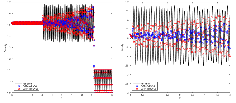
Figure 4.1. The comparison of the density profile (left) and its local enlargement (right) for the Titarev-Toro problem in Example 2. The schemes used are GRP4-WENO5 (squares) and GRP4-HWENO5 (circles) with $1000$ cells. The solid lines are the reference solution.

Example 3. Large pressure ratio problem. The large pressure ratio problem is a Riemann problem first presented in [29]. In this problem, initially the pressure and density ratio between the two neighboring states are very high. The initial data is $(\rho,v,p)=(10000,0,10000)$ for $0\leq x<0.3$ and $(\rho,v,p)=(1,0,1)$ for $0.3\leq x\leq 1.0$. The boundary condition is dealt with in the same with that in the standard Riemann problem. The output time is $t=0.12$.

An extremely strong rarefaction wave forms and it significantly affects the shock location in the numerical solution. Two factors determine the ability of a numerical scheme to properly capture the position of the shock. The first one is whether the thermodynamical effect is included in the numerical fluxes properly [12]. The second one is the numerical dissipation of the schemes. Figure 4.2 shows the density profile of the numerical solutions simulated by GRP4-WENO5 and GRP4-HWENO5 with $300$ cells. We can see that GRP4-HWENO5 behaves better due to smaller stencils and less numerical dissipations of the resulting scheme.

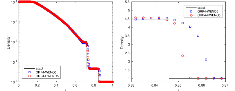
Figure 4.2. The comparison of the density profile (left) and its local enlargement (right) for the large pressure ration problem in Example 3. The schemes GRP4-WENO5 (squares) and GRP4-HWENO5 (circles) are performed with $300$ cells. The solid lines refer to the exact solution.

Example 4. The double Mach reflection problem. This is a standard test problem to display the performance of high resolution schemes. The computational domain for this problem is $[0,4]\times[0,1]$, and $[0,3]\times[0,1]$ is shown. The reflective wall lies at the bottom of the computaional domain starting from $x=\frac{1}{6}$. Initially a right-moving Mach 10 shock is positioned at $x=\frac{1}{6},y=0$ and makes a $\frac{\pi}{3}$ angle with the $x$-axis. The results are shown in Figure 4.3 from which we can see that the numerical result by GRP4-HWENO5 can resolve more structures along the slip line than that by GRP4-WENO5.

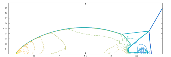
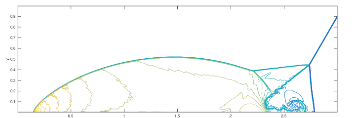
Figure 4.3. The density contours of the double Mach reflection problem in Example 4 by GRP4-WENO5 (upper) and the GRP4-HWENO5 (lower) with $960\times 240$ cells.

Example 5. Two-dimensional Riemann problems. We provide an example of two-dimensional Riemann problem taken from [6] involving the interactions of vortex sheets with rarefaction waves. The computation is implemented over the domain $[0,1]\times[0,1]$.

(4.4) $$(\rho,u,v,p)(x,y,0)=\left\{\begin{array}[]{ll}(1,0.1,0.1,1),&0.5<x<1,0.5<y<1,\\ (0.5197,-0.6259,0.1,0.4),&0<x<0.5,0.5<y<1,\\ (0.8,0.1,0.1,0.4),&0<x<0.5,0<y<0.5,\\ (0.5197,0.1,-0.6259,0.4),&0.5<x<1,0<y<0.5.\end{array}\right.$$

The output time is $0.3$.

The contours of the density and their local enlargements are shown in Figures 4.4. We can see that the scheme with the HWENO reconstruction can resolve more small structures along the vortex sheet.

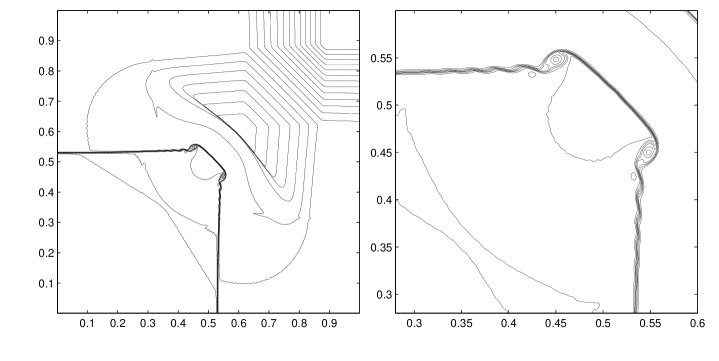
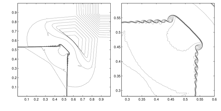
Figure 4.4. The density contours of the 2-D Riemann problem in Example 5 computed with the schemes GRP4-WENO5 (upper) and GRP4-HWENO5 (lower), respectively. $700\times 700$ cells are used.

5. Discussion

In this paper we developed a new HWENO reconstruction method just over structural (rectangular) meshes. This can be extended over unstructured meshes, but we think that the technicality may be nontrivial, which remains for future study.

A subtlety also lies in the reconstruction of spatial derivatives close to interfaces at the intermediate stage. If we would use the formulae below to interpolate the first-order derivatives as,

(5.1) $$\begin{array}[]{l}\Big{(}\displaystyle{\frac{\partial\mathbf{u}}{\partial x}}\Big{)}_{j-\frac{1}{2},+}:=\displaystyle{\frac{1}{8h}}\left(-13\bar{\mathbf{u}}_{j-1}+16\bar{\mathbf{u}}_{j}-3\bar{\mathbf{u}}_{j+1}-3h\Delta\mathbf{u}_{j-1}+h\Delta\mathbf{u}_{j+1}\right),\\[5.69054pt] \Big{(}\displaystyle{\frac{\partial\mathbf{u}}{\partial x}}\Big{)}_{j+\frac{1}{2},-}:=\displaystyle{\frac{1}{8h}}\left(3\bar{\mathbf{u}}_{j-1}-16\bar{\mathbf{u}}_{j}+13\bar{\mathbf{u}}_{j+1}+h\Delta\mathbf{u}_{j-1}-3h\Delta\mathbf{u}_{j+1}\right),\end{array}$$

the same analysis performed in Subsection 3.1 shows that the errors of $\Big{(}\displaystyle{\frac{\partial\mathbf{u}}{\partial x}}\Big{)}_{j+\frac{1}{2},\pm}$ would be $\mathcal{O}(k^{2})$ so that

$$\mathbf{f}_{j+\frac{1}{2}}^{4th}=\displaystyle\displaystyle{\frac{1}{k}}\int_{t^{n}}^{t^{n+1}}\mathbf{f}(\mathbf{u}(x_{j+\frac{1}{2}},t))dt+\mathcal{O}(k^{3}).$$

This makes the resulting scheme third-order accurate.

There is a remedy here. We could use the third order GRP solver in [19] , which is relatively complicated and we want to use an alternative method. Instead of the formulae in (5.1) to interpolate $\Big{(}\displaystyle{\frac{\partial\mathbf{u}}{\partial x}}\Big{)}^{n+\frac{1}{2}}_{j+\frac{1}{2},\pm}$, we adopt

(2.15) $$\Big{(}\displaystyle{\frac{\partial\mathbf{u}}{\partial x}}\Big{)}_{j+\frac{1}{2},\pm}:=\displaystyle{\frac{1}{12h}}\left(\bar{\mathbf{u}}_{j-1}-15\bar{\mathbf{u}}_{j}+15\bar{\mathbf{u}}_{j+1}-\bar{\mathbf{u}}_{j+2}\right)$$

in practice. Although the stencil becomes larger, the numerical results in Section 4 show that such a choice has a good practical effect.

References

• [1] M. Ben-Artzi and J. Falcovitz. A second-order Godunov-type scheme for compressible fluid dynamics. J. Comput. Phys., 55:1–32, 1984.
• [2] M. Ben-Artzi and J. Falcovitz. Generalized Riemann Problems in Computational Fluid Dynamics. Cambridge University Press, Cambridge, 2003.
• [3] M. Ben-Artzi, J. Li, and G. Warnecke. A direct Eulerian GRP scheme for compressible fluid flows. J. Comput. Phys., 218:19–43, 2006.
• [4] R. Borges, M. Carmona, B. Costa, and W. Don. An improved weighted essentially non-oscillatory scheme for hyperbolic conservation laws. Journal of Computational Physics, 227:3191–3211, 2008.
• [5] A. Christlieb, S. Gottlieb, Z. Grant, and D. Seal. Explicit strong stability preserving multistage two-derivative time-stepping schemes. J. Sci. Comput., 68:914–942, 2016.
• [6] E. Han, J. Li, and H. Tang. Accuracy of the adaptive GRP scheme and the simulation of 2-D Riemann problem for compressible Euler equations. Commun. Comput. Phys., 10(3):577–606, 2011.
• [7] A. Harten, B. Engquist, S. Osher, and S. Chakravarthy. Uniformly high-order accurate essentially nonoscillatory schemes, III. J. Comput. Phys., 71(2):231–303, 1987.
• [8] G. Jiang and C.-W. Shu. Efficient implementation of weighted ENO schemes. J. Comput. Phys., 126:202–228, 1996.
• [9] Yan Jiang, Chi-Wang Shu, and Mengping Zhang. An alternative formulation of finite difference weighted ENO schemes with Lax-Wendroff time discretization for hyperbolic conservation laws. SIAM Journal on Scientific Computing, 35(6):A1137–A1160, 2013.
• [10] P. Lax and B. Wendroff. Systems of conservation laws. Comm. Pure Appl. Math., XIII:217–237, 1960.
• [11] J. Li and Z. Du. A two-stage fourth order temporal discretization for on the Lax-Wendroff type flow solvers, I. Hyperbolic conservation laes. SIAM, J. Sci. Comput., 38:A3046–A3069, 2016.
• [12] J. Li and Y. Wang. Thermodynamical effects and high resolution methods for compressible fluid flows. J. Comput. Phys., 343:340–354, 2017.
• [13] X. D. Liu, S. Osher, and T. Chan. Weighted essentially non-oscillatory schemes. J. Comput. Phys., 115(1):200–212, 1994.
• [14] H. Luo, J. Baum, and Löhner. A Hermite WENO-based limiter for DG methods on unstructured grids. J. Comput. Phys., 225(1):686–713, 2007.
• [15] I. S. Men’shov. Increasing the order of approximation of godunov’s scheme using the solution of the generalized riemann problem. U.S.S.R. Coumput. Math. Math. Phys., 30(5):54–65, 1990.
• [16] I. S. Men’shov. Generalized problem of break-up of a single discontinuity. J. Applied Mathematics and Mechanics, 55(1):86–95, 1991.
• [17] L. Pan, K. Xu, Q. Li, and J. Li. An efficient and accurate two-stage fourth-order gas-kinetic scheme for the Euler and Navier–Stokes equations. J. Comput. Phys., 326:197–221, 2016.
• [18] K. Prendergast and K. Xu. Numerical hydrodynamics from gas-kinetic theory. J. Comput. Phys., 109:53–66, 1993.
• [19] J. Qian, J. Li, and S. Wang. The generalized Riemann problems for compressible fluid flows: Towards high order. J. Comput. Phys., 259:358–389, 2014.
• [20] J. Qiu, M. Dumbser, and C.-W. Shu. The discontinuous galerkin method with lax-wendroff type time discretizations. Computer Methods in Applied Mechanics and Engineering, 194:4528–4543, 2005.
• [21] J. Qiu and C.-W. Shu. Hermite WENO schemes and their application as limiters for Runge-Kutta discontinuous Galerkin method: one-dimensional case. J. Comput. Phys., 193:115–135, 2004.
• [22] J. Qiu and C.-W. Shu. Hermite WENO schemes and their application as limiters for Runge-Kutta discontinuous Galerkin method II: Two dimensional case. Comput. & Fluids, 34:642–663, 2005.
• [23] Jianxian Qiu and Chi-Wang Shu. Finite difference WENO schemes with Lax-Wendroff-type time discretizations. SIAM Journal on Scientific Computing, 24(6):2185–2198, 2003.
• [24] A. Quarteroni, R. Sacco, and F. Saleri. Numerical Mathematics. Springer, 2007.
• [25] C.-W. Shu. High order WENO and DG methods for time-dependent convection-dominated PDEs: A brief survey of several recent developments. J. Comput. Phys., 316:598–613, 2016.
• [26] C.-W. Shu and S. Osher. Efficient implementation of essentially nonoscillatory shock-capturing schemes, II. J. Comput. Phys., 83:32–78, 1989.
• [27] C.-W. Shu and Stanley Osher. Efficient implementation of essentially non-oscillatory shock-capturing schemes. J. Comput. Phys., 77:439–471, 1988.
• [28] Chi-Wang Shu. High order ENO and WENO schemes. In T. J. Barth and H. Deconinck, editors, High-Order Methods for Computational Physics, pages 439–582. Springer-Verlag, Berlin, 1999.
• [29] H. Tang and T. Liu. A note on the conservative schemes for the Euler equations. J. Comput. Phys., 218(1):451–459, 2006.
• [30] V. Titarev and E. Toro. Finite volume WENO schemes for three-dimensional conservation laws. J. Comput. Phys., 201:238–260, 2014.
• [31] E. F. Toro. Primitive, Conservative and Adaptive Schemes for Hyperbolic Conservation Laws, pages 323–385. Springer Netherlands, Dordrecht, 1998.
• [32] E. F. Toro and V. Titarev. Derivative Riemann solvers for systems of conservation laws and ADER methods. J. Comput. Phys., 212:150–165, 2006.
• [33] M. Ökten Turaci and Turgut Özis. Derivation of three-derivative runge-kutta methods. Numerical Algorithms, 74:247–265, 2017.