HEPHY-PUB 999/17 December 2017

GOLDSTONIC PSEUDOSCALAR MESONS
IN BETHE–SALPETER-INSPIRED SETTING
Wolfgang LUCHA
Institute for High Energy Physics,
Austrian Academy of Sciences,
Nikolsdorfergasse 18, A-1050 Vienna, Austria
Franz F. SCHÖBERL
Faculty of Physics, University of Vienna,
Boltzmanngasse 5, A-1090 Vienna, Austria
Abstract

For a two-particle bound-state equation closer to its Bethe–Salpeter origins than Salpeter’s equation, with effective-interaction kernel deliberately forged such as to ensure, in the limit of zero mass of the bound-state constituents, the vanishing of the arising bound-state mass, we scrutinize the emerging features of the lightest pseudoscalar mesons for their agreement with the behaviour predicted by a generalization of the Gell-Mann–Oakes–Renner relation.

PACS numbers: 11.10.St, 03.65.Ge, 03.65.Pm

1 Stimulus: Janiform Nature of Pseudoscalar Mesons

Within the spectrum of known elementary particles, the lowest-mass pseudoscalar mesons, the pions and kaons, occupy a unique position: On the one hand, they are understood to be quark–antiquark bound states. On the other hand, they should form the pseudo-Goldstone bosons the presence of which is necessitated by the spontaneous (and, in addition, explicit) breaking of the chiral symmetries of quantum chromodynamics (QCD). Their ambivalence renders their quantum-field-theoretic description by the Bethe–Salpeter formalism [1, 2, 3] or by suitable three-dimensional reductions of the latter, such as Salpeter’s equation [4] or the less serious simplification embodied by the bound-state equation of Ref. [5], a delicate task.

Recently, by means of a dedicated inversion technique [6], we embarked on a systematic exploration of the effective interactions between bound-state constituents entering, in form of configuration-space central potentials $V(r),$ $r\equiv|\bm{x}|,$ in Salpeter’s approach [7, 8, 9, 10] or our softened approximation [11, 12, 13]. Here, we demonstrate how the reliability of predictions for such a meson is judged by their fulfilment of Gell-Mann–Oakes–Renner-type relationships.

There is no need to announce in detail the expectable outline of this paper: By applying the “Bethe–Salpeter-inspired” bound-state formalism constructed in Ref. [5] (Sec. 2) to the lowest pseudoscalar mesons (Sec. 3), some of their thus predicted basic features (Sec. 4) are examined, for the Goldstone-friendly interquark potential derived in Ref. [11] (Sec. 5), with regard to their compatibility with relationships of Gell-Mann–Oakes–Renner type (Sec. 6). Throughout this paper, we use the natural units of relativistic quantum physics: $\hbar=c=1.$

2 Bethe–Salpeter Formalism: an Instantaneous Limit

In principle, the Bethe–Salpeter formalism [1, 2, 3] is the proper tool for a Poincaré-covariant description of bound states within the framework of relativistic quantum field theories: the homogeneous Bethe–Salpeter equation relates the Bethe–Salpeter amplitude, encoding the distribution of the relative momenta of the bound-state constituents, to, for $n$ constituents, their $n$ propagators and the ($2\,n$)-point Green function encompassing all their interactions.

We intend to deal with mesons, so we let $n=2$ and focus to bound states composed of a fermion and an antifermion. In terms of the individual coordinates and momenta of the two bound-state constituents, discriminated by the subscript $i=1,2$, parameters $\eta_{1,2}\in\mathbb{R},$ and the center-of-momentum and relative coordinates and total and relative momenta given by

$$X \equiv\eta_{1}\,x_{1}+\eta_{2}\,x_{2}\ , x \equiv x_{1}-x_{2}\ , \eta_{1}+\eta_{2} =1\ ,$$

$$P \equiv p_{1}+p_{2}\ , p \equiv\eta_{2}\,p_{1}-\eta_{1}\,p_{2}\ , P^{2} =\widehat{M}^{2}\ ,$$

the momentum-space Bethe–Salpeter amplitude of each such bound state $|{\rm B}(P)\rangle$ is defined by the Fourier transform of the vacuum-to-bound-state matrix element of the time-ordered product of the field operators $\psi_{i}(x_{i})$ of both involved bound-state constituents according to

$$\Phi(p,P)\equiv\exp({\rm i}\,P\,X)\int{\rm d}^{4}x\exp({\rm i}\,p\,x)\,\langle 0|{\rm T}(\psi_{1}(x_{1})\,\bar{\psi}_{2}(x_{2}))|{\rm B}(P)\rangle\ .$$

By Poincaré covariance, the propagator of any fermion $i$ is fixed by only two Lorentz-scalar functions, interpretable as, e.g., its mass $M_{i}(p^{2})$ and wave-function renormalization $Z_{i}(p^{2})$:

$$S_{i}(p)=\frac{{\rm i}\,Z_{i}(p^{2})}{\not\!p-M_{i}(p^{2})+{\rm i}\,\varepsilon}\ ,\qquad\not\!p\equiv p^{\mu}\,\gamma_{\mu}\ ,\qquad\varepsilon\downarrow 0\ ,\qquad i=1,2\ .$$ (1)

As a relativistic formalism, however, the Bethe–Salpeter approach to bound states is, in general, threatened by the (possible) appearance of excitations in the relative-time variable of the bound-state constituents. Lacking nonrelativistic counterparts, the interpretation of such solutions poses a severe challenge. This obstacle to the light-hearted application of the Bethe–Salpeter approach to relativistic bound-state problems triggered the construction of approximations not plagued by timelike excitations: By seeking suitable three-dimensional reductions of the Poincaré-covariant framework by constructing instantaneous limits of the homogeneous Bethe–Salpeter formalism, bound-state equations for the Salpeter amplitude

$$\phi(\bm{p})\equiv\int\frac{{\rm d}p_{0}}{2\pi}\,\Phi(p,P)$$

have been proposed. The supposedly simplest among all these is the one due to Salpeter [4], who assumed, for all bound-state constituents, both constant masses and free propagation.

Some time ago, in an attempt to overcome some of the limitations induced by Salpeter’s assumption [4] of strict constancy of the masses of all bound-state constituents by retaining as much as feasible from the dynamical information encrypted in the momentum behaviour of (fermion) propagator functions, we formulated an approximation [5] to the homogeneous Bethe–Salpeter equation which is characterized by the ignorance of merely the dependence of both propagator functions on the time components of the involved momentum variables. Recalling free Hamiltonian, free energy and energy projection operators of fermion $i=1,2,$

$$H_{i}(\bm{p})\equiv\gamma_{0}\,[\bm{\gamma}\cdot\bm{p}+M_{i}(\bm{p}^{2})]\ ,\qquad E_{i}(\bm{p})\equiv\sqrt{\bm{p}^{2}+M_{i}^{2}(\bm{p}^{2})}\ ,\qquad\Lambda_{i}^{\pm}(\bm{p})\equiv\frac{E_{i}(\bm{p})\pm H_{i}(\bm{p})}{2\,E_{i}(\bm{p})}\ ,$$

the resulting instantaneous-limit equation [5] governing fermion–antifermion bound states, with three-momentum $\bm{P}$ and mass generically labelled by $\widehat{M},$ can be cast [14, 11, 13, 15], in the center-of-momentum frame of such bound states, that is, for $\bm{P}=\bm{p}_{1}+\bm{p}_{2}=0$, into the form

$$\phi(\bm{p})=Z_{1}(\bm{p}^{2})\,Z_{2}(\bm{p}^{2})\left(\frac{\Lambda_{1}^{+}(\bm{p})\,\gamma_{0}\,I(\bm{p})\,\Lambda_{2}^{-}(\bm{p})\,\gamma_{0}}{\widehat{M}-E_{1}(\bm{p})-E_{2}(\bm{p})}-\frac{\Lambda_{1}^{-}(\bm{p})\,\gamma_{0}\,I(\bm{p})\,\Lambda_{2}^{+}(\bm{p})\,\gamma_{0}}{\widehat{M}+E_{1}(\bm{p})+E_{2}(\bm{p})}\right),$$ (2)

where an integral kernel $K(\bm{p},\bm{q})$ subsumes the, by assumption instantaneous, interactions:

$$I(\bm{p})\equiv\int\frac{{\rm d}^{3}q}{(2\pi)^{3}}\,K(\bm{p},\bm{q})\,\phi(\bm{q})\ .$$ (3)

The normalization of any state $|B(\bm{P})\rangle$ may be defined by a normalization factor $N(P);$ popular choices of $N(P)$ are relativistically noncovariant normalizations such as $N(P)=1$ and $N(P)=(2\pi)^{3},$ or a relativistically covariant normalization such as $N(P)=(2\pi)^{3}\,2\,P_{0}$:

$$\langle B(\bm{P})|B(\bm{P}^{\prime})\rangle=N(P)\,\delta^{(3)}(\bm{P}-\bm{P}^{\prime})\ .$$ (4)

Bound-state normalization $N(P)$ and Salpeter-amplitude norm $\|\phi\|$ are related via [16, 17, 18, 19]

$$\|\phi\|^{2}=\frac{N(P)}{(2\pi)^{3}}\ .$$

Now, neglecting in the covariant normalization condition for the Bethe–Salpeter amplitude $\Phi(p,P)$ the dependence of the Bethe–Salpeter interaction kernel on the bound state’s total four-momentum $P$ or assuming that, in the center-of-momentum frame of the bound state, the instantaneous version of the interaction kernel does not depend on $P,$ the norm of each Salpeter amplitude $\phi(\bm{p})$ is given by (e.g., Refs. [17, Eq. (2.9)], [18, Eq. (29)] or [19, Eq. (9)])

$$\|\phi\|^{2} =\frac{1}{2}\int\frac{{\rm d}^{3}p}{(2\pi)^{3}}\,{\rm Tr}\!\left[\phi^{\dagger}(\bm{p})\left(\frac{H_{1}(\bm{p})}{E_{1}(\bm{p})}\,\phi(\bm{p})-\phi(\bm{p})\,\frac{H_{2}(-\bm{p})}{E_{2}(\bm{p})}\right)\right]$$

$$=\int\frac{{\rm d}^{3}p}{(2\pi)^{3}}\,{\rm Tr}\!\left[\phi^{\dagger}(\bm{p})\,\frac{H_{1}(\bm{p})}{E_{1}(\bm{p})}\,\phi(\bm{p})\right],$$

where the trace clearly extends over all colour, flavour, and spinor degrees of freedom of the bound-state constituents. In view of the fact that our mesonic bound states, $|B\rangle,$ are colour singlets, this normalization of the Bethe–Salpeter amplitude $\Phi(p,P)$ with respect to colour induces, in the general case of $N_{\rm c}$ colour degrees of freedom, an overall colour factor $1/\sqrt{N_{\rm c}}.$

We assume a kind of flavour symmetry of all fermion propagators in our Bethe–Salpeter formalism, manifesting in form of equality of the Lorentz-scalar functions of the same kind:

$$Z_{1}(\bm{p}^{2})=Z_{2}(\bm{p}^{2})=Z(\bm{p}^{2})\ ,\qquad M_{1}(\bm{p}^{2})=M_{2}(\bm{p}^{2})=M(\bm{p}^{2})\ .$$

This, in turn, implies for the Dirac Hamiltonians, kinetic energies and projection operators

$$H_{1}(\bm{p})=H_{2}(\bm{p})=H(\bm{p}) \equiv\gamma_{0}\,[\bm{\gamma}\cdot\bm{p}+M(\bm{p}^{2})]\ ,$$

$$E_{1}(\bm{p})=E_{2}(\bm{p})=E(\bm{p}) \equiv\sqrt{\bm{p}^{2}+M^{2}(\bm{p}^{2})}\ ,$$

$$\Lambda_{1}^{\pm}(\bm{p})=\Lambda_{2}^{\pm}(\bm{p})=\Lambda^{\pm}(\bm{p}) \equiv\frac{E(\bm{p})\pm H(\bm{p})}{2\,E(\bm{p})}\ ,$$

and serves to simplify our fermion–antifermion bound-state equation (2) a little bit further:

$$\phi(\bm{p})=Z^{2}(\bm{p}^{2})\left(\frac{\Lambda^{+}(\bm{p})\,\gamma_{0}\,I(\bm{p})\,\Lambda^{-}(\bm{p})\,\gamma_{0}}{\widehat{M}-2\,E(\bm{p})}-\frac{\Lambda^{-}(\bm{p})\,\gamma_{0}\,I(\bm{p})\,\Lambda^{+}(\bm{p})\,\gamma_{0}}{\widehat{M}+2\,E(\bm{p})}\right).$$ (5)

The latter variant of instantaneous Bethe–Salpeter equation shall be used, in the following, to study those basic features of the pseudo-Goldstone-type pseudoscalar mesons that enter in the Gell-Mann–Oakes–Renner relation [21] or a more modern generalization thereof [22].

3 Spin-Singlet Fermion–Antifermion Bound Systems

By definition, any pseudoscalar bound state of a spin-$\frac{1}{2}$ fermion and a spin-$\frac{1}{2}$ antifermion is characterized by zero bound-state spin $J,$ $J=0,$ and negative parity $P,$ $P=-1.$ Thus, any such state perforce has zero relative orbital angular momentum $\ell,$ $\ell=0,$ and zero total spin $S,$ $S=0$ (e.g., Ref. [23]). The latter, in turn, implies that any such state must have positive charge-conjugation parity $C,$ $C=+1,$ while the product of $P$ and $C$ is negative: $C\,P=-1;$ necessarily, the spin–parity–charge-conjugation assignment of such state reads $J^{PC}=0^{-+}.$

The most general Salpeter amplitude $\phi(\bm{p})$ of a spin-singlet fermion–antifermion bound state is defined, in its center-of-momentum frame, by two independent components $\varphi_{1,2}(\bm{p})$:

$$\phi(\bm{p})=\frac{1}{\sqrt{N_{\rm c}}}\left[\varphi_{1}(\bm{p})\,\frac{H(\bm{p})}{E(\bm{p})}+\varphi_{2}(\bm{p})\right]\gamma_{5}\ .$$ (6)

In terms of these Salpeter components, our bound-state normalization $N(P)$ introduced in Eq. (4) becomes, in accordance with, e.g., Refs. [17, Eq. (4.13)] and [19, Eqs. (18) and (26)],

$$N(P)=(2\pi)^{3}\,\|\phi\|^{2} =4\int{\rm d}^{3}p\,[\varphi_{1}^{\ast}(\bm{p})\,\varphi_{2}(\bm{p})+\varphi_{2}^{\ast}(\bm{p})\,\varphi_{1}(\bm{p})]$$

$$=4\int\limits_{0}^{\infty}{\rm d}p\,p^{2}\,[\varphi_{1}^{\ast}(p)\,\varphi_{2}(p)+\varphi_{2}^{\ast}(p)\,\varphi_{1}(p)]\ ,\qquad p\equiv|\bm{p}|\ ;$$ (7)

here, the last equality gives the norm in terms of the radial factors $\varphi_{1,2}(p)$ obtained as relics of the Salpeter components $\varphi_{1,2}(\bm{p})$ by factorizing out any dependence on angular variables.

In the interaction term (3), the integral kernel $K(\bm{p},\bm{q})$ acting on the Salpeter amplitude $\phi(\bm{p})$ reflects Lorentz nature and strength of the effective interactions between bound-state constituents by generalized Dirac matrices $\Gamma$ and Lorentz-scalar functions $V(\bm{p},\bm{q}).$ As long as not knowing better, we assume for fermion and antifermion identical effective couplings,

$$K(\bm{p},\bm{q})\,\phi(\bm{q})=\sum_{\Gamma}V_{\Gamma}(\bm{p},\bm{q})\,\Gamma\,\phi(\bm{q})\,\Gamma\ ,$$

and the integral kernel to exhibit Fierz symmetry, realized, for instance, by choosing for the tensor structure $\Gamma\otimes\Gamma$ a single linear combination of vector, pseudoscalar, and scalar terms:

$$\Gamma\otimes\Gamma=\frac{1}{2}\,(\gamma_{\mu}\otimes\gamma^{\mu}+\gamma_{5}\otimes\gamma_{5}-1\otimes 1)\ .$$ (8)

Given that the interaction term (3) is of convolution type and respects spherical symmetry, which is assured if $K(\bm{p},\bm{q})=K((\bm{p}-\bm{q})^{2})$ or $V_{\Gamma}(\bm{p},\bm{q})=V_{\Gamma}((\bm{p}-\bm{q})^{2})$ holds, our bound-state equation (5) with Dirac structure (8) can be boiled down to an eigenvalue problem with the bound-state masses $\widehat{M}$ as its eigenvalues, posed by a coupled system of one integral and one algebraic equation, which provides the radial factors $\varphi_{1,2}(p)$ in the components $\varphi_{1,2}(\bm{p})$ [24]:

$$2\,E(p)\,\varphi_{2}(p)+2\,Z^{2}(p^{2})\int\limits_{0}^{\infty}\frac{{\rm d}q\,q^{2}}{(2\pi)^{2}}\,V(p,q)\,\varphi_{2}(q)=\widehat{M}\,\varphi_{1}(p)\ ,$$ (9a)

$$2\,E(p)\,\varphi_{1}(p)=\widehat{M}\,\varphi_{2}(p)\ ,$$ (9b)

with the interaction potential $V(r)$ sought entering via its double Fourier–Bessel transform

$$V(p,q)\equiv\frac{8\pi}{p\,q}\int\limits_{0}^{\infty}{\rm d}r\sin(p\,r)\sin(q\,r)\,V(r)\ ,\qquad q\equiv|\bm{q}|\ .$$

When solving the coupled equations (9a) and (9b), we shall make a distinction of two cases:

• For $\widehat{M}=0,$ Eq. (9b) implies $\varphi_{1}(\bm{p})=0,$ whence the Salpeter amplitude (6) reduces to

  $$\phi(\bm{p})=\frac{1}{\sqrt{N_{\rm c}}}\,\varphi_{2}(\bm{p})\,\gamma_{5}\ ,$$

  with the radial behaviour of its nonvanishing component $\varphi_{2}(\bm{p})$ governed by Eq. (9a):

  $$E(p)\,\varphi_{2}(p)+Z^{2}(p^{2})\int\limits_{0}^{\infty}\frac{{\rm d}q\,q^{2}}{(2\pi)^{2}}\,V(p,q)\,\varphi_{2}(q)=0\ .$$ (10)

• For $\widehat{M}\neq 0,$ insertion of one of the two relations (9a) and (9b) into the other entails an eigenvalue problem for eigenvalues ${\widehat{M}}^{2},$ equivalently defined by either of the relations

  $$4\,E^{2}(p)\,\varphi_{1}(p)+4\,Z^{2}(p^{2})\int\limits_{0}^{\infty}\frac{{\rm d}q\,q^{2}}{(2\pi)^{2}}\,V(p,q)\,E(q)\,\varphi_{1}(q) ={\widehat{M}}^{2}\,\varphi_{1}(p)\ ,$$ (11a)

  $$4\,E^{2}(p)\,\varphi_{2}(p)+4\,Z^{2}(p^{2})\,E(p)\int\limits_{0}^{\infty}\frac{{\rm d}q\,q^{2}}{(2\pi)^{2}}\,V(p,q)\,\varphi_{2}(q) ={\widehat{M}}^{2}\,\varphi_{2}(p)\ .$$ (11b)

Expressed, on an equal footing, in terms of radial factor $\varphi_{1}(p)$ or $\varphi_{2}(p)$ and abbreviating by

$$K_{1}^{2}\equiv\int\limits_{0}^{\infty}{\rm d}p\,p^{2}\,E(p)\,|\varphi_{1}(p)|^{2}\ ,\qquad K_{2}^{2}\equiv\int\limits_{0}^{\infty}{\rm d}p\,p^{2}\,\frac{|\varphi_{2}(p)|^{2}}{E(p)}$$

the arising integrals, the use of relation (9b) translates the normalization condition (7) into

$$16\,\frac{\operatorname{Re}(\widehat{M})}{|\widehat{M}|^{2}}\,K_{1}^{2}=4\,\operatorname{Re}(\widehat{M})\,K_{2}^{2}=N(P)\ .$$

Here, we take into account the possibility that, without established self-adjointness, the set of solutions to static reductions of the form (2) might include non-real mass eigenvalues $\widehat{M}.$

4 Lowest-Lying Pseudoscalar Mesons: Basic Features

The mass eigenvalues of all states in the physical sector of solutions must be real. Hence, for our intended analysis of ground-state pseudoscalar mesons we feel safe to assume $\widehat{M}^{\ast}=\widehat{M}.$ Retaining the normalization $N(P)$ in Eq. (4) unspecified, we refrain from sticking to a fixed choice of normalization and introduce, for arbitrary $N(P),$ the two features of ground-state pseudoscalar mesons that the generalized Gell-Mann–Oakes–Renner relation [22] entwines:

1. The decay constant $f_{B}$ for a generic pseudoscalar meson $B$ regarded as bound state of quark and antiquark with field operators $\psi_{1,2}(X)$ parametrizes the vacuum-to-bound state matrix element of the weak axial-vector current $A_{\mu}(X)\equiv{:\!\bar{\psi}_{1}(X)\,\gamma_{\mu}\,\gamma_{5}\,\psi_{2}(X)\!:},$

   $$\langle 0|A_{\mu}(X)|B(P)\rangle={\rm i}\,\frac{\sqrt{N(P)}}{(2\pi)^{3/2}\,\sqrt{2\,P_{0}}}\,f_{B}\,P_{\mu}\exp(-{\rm i}\,P\,X)\ ,$$

   and is thus inferred by projecting the Salpeter amplitude of $B$ onto the current $A_{0}(0)$:

   $$f_{B}=\frac{{\rm i}}{(2\pi)^{3/2}\,\sqrt{N(P)}}\,\sqrt{\frac{2}{\widehat{M}}}\int{\rm d}^{3}p\,{\rm Tr}[\gamma_{0}\,\gamma_{5}\,\phi(\bm{p})]\ .$$

   Use of Eq. (6) allows us to reshape $f_{B}$ to the (trivially equivalent) more explicit forms

   $$f_{B}=-\frac{{\rm i}\,\sqrt{N_{\rm c}}}{\pi\,K_{1}}\int\limits_{0}^{\infty}{\rm d}p\,p^{2}\,\frac{M(p^{2})}{E(p)}\,\varphi_{1}(p)=-\frac{{\rm i}\,\sqrt{N_{\rm c}}}{\pi\,K_{2}}\int\limits_{0}^{\infty}{\rm d}p\,p^{2}\,\frac{M(p^{2})}{E^{2}(p)}\,\varphi_{2}(p)\ .$$

   Both forms clearly reveal that, for the specific Bethe–Salpeter model considered here, there is no explicit dependence of this decay constant $f_{B}$ on the bound-state mass $\widehat{M}.$

2. Likewise, we define, for a pseudoscalar meson $B,$ the associated in-hadron condensate [22] ${\mathbb{C}}_{B}$ by the vacuum-to-bound state matrix element of the density $:\!\bar{\psi}_{1}(0)\,\gamma_{5}\,\psi_{2}(0)\!:$,

   $$\frac{\sqrt{N(P)}}{(2\pi)^{3/2}\,\sqrt{2\,P_{0}}}\,{\mathbb{C}}_{B}\equiv\langle 0|{:\!\bar{\psi}_{1}(0)\,\gamma_{5}\,\psi_{2}(0)\!:}|B(P)\rangle\ .$$

   Paralleling the $f_{B}$ case, this condensate is found by projection onto the latter density,

   $${\mathbb{C}}_{B}=-\sqrt{\frac{2\,\widehat{M}}{(2\pi)^{3}\,N(P)}}\int{\rm d}^{3}p\,{\rm Tr}[\gamma_{5}\,\phi(\bm{p})]\ ,$$

   and, recalling $\phi(\bm{p})$ of Eq. (6), reduces to the (clearly equivalent) explicit expressions

   $${\mathbb{C}}_{B}=-\frac{2\,\sqrt{N_{\rm c}}}{\pi\,K_{1}}\int\limits_{0}^{\infty}{\rm d}p\,p^{2}\,E(p)\,\varphi_{1}(p)=-\frac{2\,\sqrt{N_{\rm c}}}{\pi\,K_{2}}\int\limits_{0}^{\infty}{\rm d}p\,p^{2}\,\varphi_{2}(p)\ .$$

With these definitions of decay constant $f_{B}$ and in-hadron condensate ${\mathbb{C}}_{B}$ of a pseudoscalar meson $B$ and $m$ denoting the (by assumption, equal) mass parameters of its constituents in the QCD Lagrangian, the modernized Gell-Mann–Oakes–Renner relation of Ref. [22] reads

$$f_{B}\,\widehat{M}_{B}^{2}=2\,m\,{\mathbb{C}}_{B}\ ,$$ (12)

as a direct consequence of the renormalized axial-vector Ward–Takahashi identity of QCD. (For practical reasons, we suppress here any reference to issues related to renormalization.)

5 Inversion of Dyson–Schwinger Propagator Solution

At this stage, merely a sole ingredient to our three-dimensional bound-state equation (2) is still lacking: the form of the Lorentz-scalar potential function $V(\bm{p},\bm{q})$ capable of describing Goldstonic pseudoscalar quark–antiquark bound states. As demonstrated in Refs. [6, 8, 9, 10, 11], our bound-state framework is sufficiently simple to allow, by means of inversion techniques, for easy determination of these effective interactions from some knowledge about solutions.

In the chiral limit, definable, for QCD, by the vanishing of the quark-mass parameter in its Lagrangian, the renormalized axial-vector Ward–Takahashi identity of QCD relates the center-of-momentum Bethe–Salpeter amplitude $\Phi(p,0)$ for the massless flavour-nonsinglet pseudoscalar mesons to the quark propagator $S(p)$ [22]. In Euclidean-space representation, indicated by underlining the corresponding variables, this relation between Bethe–Salpeter amplitude and the quark propagator functions $M(\underline{k}^{2})$ and $Z(\underline{k}^{2})$ can be reformulated as [8]

$$\Phi(\underline{k},0)\propto\frac{Z(\underline{k}^{2})\,M(\underline{k}^{2})}{\underline{k}^{2}+M^{2}(\underline{k}^{2})}\,\underline{\gamma}_{5}+\mbox{subleading contributions}\ .$$

This relation can be capitalized to convert, by inversion [6], knowledge about the behaviour of the fermion propagator into information about the underlying effective quark–antiquark interactions [7, 8, 9, 10, 11, 12, 13]. In Ref. [11], exploiting the chiral-limit solution to the Dyson–Schwinger equation for the quark propagator based on a phenomenologically acceptable model for the four-point Green function serving as required Bethe–Salpeter interaction-kernel input [26], we extracted, from the quark-propagator functions reproduced in Fig. 1, the potential $V(r)$ given in Fig. 2, showing quark confinement by rising from slightly negative $V(0)$ to infinity.

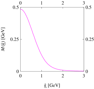
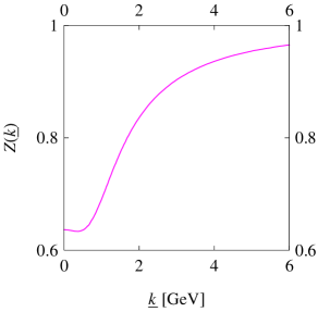
(a)	(b)

Figure 1: Dyson–Schwinger solution [26] for the full quark propagator (1) in the chiral limit (depicted vs. $\underline{k}\equiv(\underline{k}^{2})^{1/2}$ [27]): (a) mass $M(\underline{k})$ and (b) wave-function renormalization $Z(\underline{k})$.

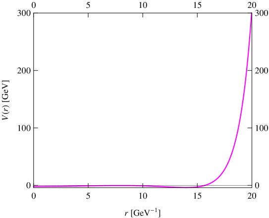
Figure 2: Configuration-space potential $V(r)$ [11] found upon inverting the Bethe–Salpeter problem (10) for a Salpeter amplitude (6) fixed by the quark propagator functions of Fig. 1.

6 Gell-Mann–Oakes–Renner-Related Characteristics

By use of, e.g., the standard solution methods sketched in App. A, it is now straightforward to harvest the findings of our bound-state formalism for the pseudoscalar-meson properties of interest. In order to track the latter’s behaviour with increasing quark mass $m,$ we mimic finite values of $m$ by exploiting the propagator solutions provided in Ref. [27, Fig. 1] for the light quarks $q=u,d,s.$ The predicted properties of the generic pseudoscalar meson defined thereby, collected in Table 1, exhibit satisfactory agreement with the qualitative behaviour expected from the Gell-Mann–Oakes–Renner-type relation (12): Within the errors induced by the details of our treatment of the information extracted pointwise from Ref. [27, Fig. 1], our fictitious-meson mass squared $\widehat{M}_{B}^{2}$ vanishes in the chiral limit $m=0$ and rises with $m.$ Moreover, we get a reasonable proximity of the size of quark masses deduced from Eq. (12),

$$m=\frac{f_{B}\,\widehat{M}_{B}^{2}}{2\,{\mathbb{C}}_{B}}\ ,$$

to the PDG averages [28] (at a renormalization scale $\mu=2\;\mbox{GeV}$) of the light current-quark masses $\overline{m}_{q}(\mu)$ obtained in the modified minimal-subtraction ($\overline{\rm MS}$) renormalization scheme,

$$\frac{\overline{m}_{u}+\overline{m}_{d}}{2}(2\;\mbox{GeV})=\left(3.5^{+0.7}_{-0.3}\right)\mbox{MeV}\ ,\qquad\overline{m}_{s}(2\;\mbox{GeV})=\left(96^{+8}_{-4}\right)\mbox{MeV}\ .$$

In summary, we conclude to have achieved the envisaged proof of feasibility. Describing the lowest pseudoscalar mesons by an advanced instantaneous Bethe–Salpeter equation [5] with an effective interaction designed to reproduce these mesons’ Goldstone nature [11], we gain numerical predictions for a couple of fundamental properties of these quark–antiquark bound states which, to say the least, are of the (experimentally) correct order of magnitude and comply with the nature of their interrelationship dictated by QCD on general grounds.

Appendix A Matrix Representations of Bound-State Equations

The solutions to an explicit eigenvalue problem of the kind posed by our radial bound-state equations (11a) and (11b) can be, in principle, straightforwardly determined by conversion to equivalent matrix eigenvalue problems, accomplished by expansion of the eigenfunctions sought and, if necessary, related quantities over some basis of the respective function space. For instance, by expanding, in terms of basis functions $\chi_{i}(r)$ in configuration space or $\widetilde{\chi}_{i}(p)$ in momentum space ($i\in\mathbb{N}$), our Salpeter function $\varphi_{2}(p)$, with coefficients $c_{i}$, and the terms $Z^{2}(p^{2})\,E(p)\,\widetilde{\chi}_{i}^{*}(p)$, the bound-state equation (11b) governing $\varphi_{2}(p)$ becomes the eigenvalue equation of a matrix ${\mathbb{O}}=({\mathbb{O}}_{ij}),$ defined by kinetic elements ${\mathbb{T}}_{ij}$ and potential elements ${\mathbb{V}}_{kj}$:

$$\varphi_{2}(p)=\sum_{i=0}^{N<\infty}c_{i}\,\widetilde{\chi}_{i}(p)\qquad\Longrightarrow\qquad\sum_{j=0}^{N<\infty}{\mathbb{O}}_{ij}\,c_{j}={\widehat{M}}^{2}\,c_{i}\ ,\qquad{\mathbb{O}}_{ij}=4\,{\mathbb{T}}_{ij}+4\sum_{k=0}^{N<\infty}d_{ik}\,{\mathbb{V}}_{kj}\ ,$$

$$\quad{\mathbb{T}}_{ij}\equiv\int\limits_{0}^{\infty}{\rm d}p\,p^{2}\,\widetilde{\chi}_{i}^{*}(p)\,E^{2}(p)\,\widetilde{\chi}_{j}(p)\ ,\qquad{\mathbb{V}}_{ij}\equiv\int\limits_{0}^{\infty}{\rm d}r\,r^{2}\,\chi_{i}^{*}(r)\,V(r)\,\chi_{j}(r)\ ,$$

$$\quad d_{ij}\equiv\int\limits_{0}^{\infty}{\rm d}p\,p^{2}\,\widetilde{\chi}_{i}^{*}(p)\,Z^{2}(p^{2})\,E(p)\,\widetilde{\chi}_{j}(p)\qquad\Longleftrightarrow\qquad Z^{2}(p^{2})\,E(p)\,\widetilde{\chi}_{i}^{*}(p)=\sum_{j=0}^{N<\infty}d_{ij}\,\widetilde{\chi}_{j}^{*}(p)\ .$$

Accordingly, it proves advantageous to employ a basis that may be represented analytically in configuration and momentum space. In the past [29, 30, 31, 32, 33, 34, 35, 36], we found it rather convenient to span the Hilbert space $L_{2}(\mathbb{R}^{+})$ of with weight $x^{2}$ square-integrable functions on the positive real line $\mathbb{R}^{+}$ by an orthonormalized basis that involves the generalized-Laguerre orthogonal polynomials $L_{i}^{(\gamma)}(x)$ for parameter $\gamma>-1$ [37, 38], and a variational parameter $\mu\in(0,\infty)$:

$$\chi_{i}(r) =\sqrt{\frac{(2\,\mu)^{3}\,i!}{\Gamma(i+3)}}\exp(-\mu\,r)\,L_{i}^{(2)}(2\,\mu\,r)\ ,\qquad L_{i}^{(\gamma)}(x)\equiv\sum_{t=0}^{i}\binom{i+\gamma}{i-t}\frac{(-x)^{t}}{t!}\ ,$$

$$\widetilde{\chi}_{i}(p) =4\,\sqrt{\frac{\mu^{3}\,i!}{\pi\,\Gamma(i+3)}}\,\sum_{t=0}^{i}\,\frac{(-1)^{t}}{t!}\binom{i+2}{i-t}\frac{\Gamma(t+2)\,(2\,\mu)^{t}}{p\,(p^{2}+\mu^{2})^{t/2+1}}\sin\!\left[(t+2)\arctan\frac{p}{\mu}\right],$$

$$\int\limits_{0}^{\infty}{\rm d}r\,r^{2}\,\chi_{i}(r)\,\chi_{j}(r)=\int\limits_{0}^{\infty}{\rm d}p\,p^{2}\,\widetilde{\chi}_{i}^{*}(p)\,\widetilde{\chi}_{j}(p)=\delta_{ij}\ ,\qquad i,j=0,1,2,\dots\ .$$

Table 1: Results for bound-state mass $\widehat{M},$ decay constant $f_{B},$ and in-hadron condensate ${\mathbb{C}}_{B}$ of our description of lightest pseudoscalar mesons defined by Eqs. (5) and (8) together with the effective potential of Fig. 2, for the three light-quark scenarios of Ref. [26], as well as the quark mass parameter $m$ fitting to the generalized Gell-Mann–Oakes–Renner relation (12).

Constituents	$\widehat{M}\;[\mbox{MeV}]$	$f_{B}\;[\mbox{MeV}]$	${\mathbb{C}}_{B}\;[\mbox{GeV}^{2}]$	$m\;[\mbox{MeV}]$
chiral quarks	6.8	151	0.585	$0.0059$
$u$/$d$ quarks	148.6	155	0.598	$2.85$
$s$ quarks	620.7	211	0.799	$51.0$

References

- [1] H. A. Bethe and E. E. Salpeter, Phys. Rev. 82 (1951) 309.
- [2] M. Gell-Mann and F. Low, Phys. Rev. 84 (1951) 350.
- [3] E. E. Salpeter and H. A. Bethe, Phys. Rev. 84 (1951) 1232.
- [4] E. E. Salpeter, Phys. Rev. 87 (1952) 328.
- [5] W. Lucha and F. F. Schöberl, J. Phys. G: Nucl. Part. Phys. 31 (2005) 1133, arXiv:hep-th/0507281.
- [6] W. Lucha and F. F. Schöberl, Phys. Rev. D 87 (2013) 016009, arXiv:1211.4716 [hep-ph].
- [7] W. Lucha, Proc. Sci., EPS-HEP 2013 (2013) 007, arXiv:1308.3130 [hep-ph].
- [8] W. Lucha and F. F. Schöberl, Phys. Rev. D 92 (2015) 076005, arXiv:1508.02951 [hep-ph].
- [9] W. Lucha and F. F. Schöberl, Phys. Rev. D 93 (2016) 056006, arXiv:1602.02356 [hep-ph].
- [10] W. Lucha and F. F. Schöberl, Phys. Rev. D 93 (2016) 096005, arXiv:1603.08745 [hep-ph].
- [11] W. Lucha and F. F. Schöberl, Int. J. Mod. Phys. A 31 (2016) 1650202, arXiv:1606.04781 [hep-ph].
- [12] W. Lucha, EPJ Web Conf. 129 (2016) 00047, arXiv:1607.02426 [hep-ph].
- [13] W. Lucha, EPJ Web Conf. 137 (2017) 13009, arXiv:1609.01474 [hep-ph].
- [14] W. Lucha and F. F. Schöberl, in XII International Conference on Hadron Spectroscopy — Hadron 07, edited by L. Benussi, M. Bertani, S. Bianco, C. Bloise, R. de Sangro, P. de Simone, P. di Nezza, P. Gianotti, S. Giovannella, M. P. Lombardo, and S. Pacetti, Frascati Phys. Ser. No. C07-10-08 Vol. 46 (INFN, Laboratori Nazionali di Frascati, Frascati, Italy, 2007), p. 1539, arXiv:0711.1736 [hep-ph].
- [15] W. Lucha, in QCD@Work 2010: International Workshop on Quantum Chromodynamics: Theory and Experiment — Beppe Nardulli Memorial Workshop, edited by L. Angelini, G. E. Bruno, P. Colangelo, D. Creanza, F. De Fazio, and E. Nappi, AIP Conf. Proc. No. 1317 (AIP, New York, 2010), p. 122, arXiv:1008.1404 [hep-ph].
- [16] A. Le Yaouanc, L. Oliver, S. Ono, O. Pène, and J.-C. Raynal, Phys. Rev. D 31 (1985) 137.
- [17] J.-F. Lagaë, Phys. Rev. D 45 (1992) 305.
- [18] J. Resag, C. R. Münz, B. C. Metsch, and H. R. Petry, Nucl. Phys. A 578 (1994) 397, arXiv:nucl-th/9307026.
- [19] M. G. Olsson, S. Veseli, and K. Williams, Phys. Rev. D 52 (1995) 5141, arXiv:hep-ph/9503477.
- [20] C. H. Llewellyn Smith, Ann. Phys. (N.Y.) 53 (1969) 521.
- [21] M. Gell-Mann, R. J. Oakes, and B. Renner, Phys. Rev. 175 (1968) 2195.
- [22] P. Maris, C. D. Roberts, and P. C. Tandy, Phys. Lett. B 420 (1998) 267, arXiv:nucl-th/9707003.
- [23] W. Lucha, F. F. Schöberl, and D. Gromes, Phys. Rep. 200 (1991) 127.
- [24] Z.-F. Li, W. Lucha, and F. F. Schöberl, Phys. Rev. D 76 (2007) 125028, arXiv:0707.3202 [hep-ph].
- [25] T. Hilger, M. Gómez-Rocha, A. Krassnigg, and W. Lucha, Eur. Phys. J. A 53 (2017) 213, arXiv:1702.06262 [hep-ph].
- [26] P. Maris and P. C. Tandy, Phys. Rev. C 60 (1999) 055214, arXiv:nucl-th/9905056.
- [27] P. Maris, in Proceedings of the International Conference on Quark Confinement and the Hadron Spectrum IV, editors W. Lucha and K. Maung Maung (World Scientific, Singapore, 2002), p. 163, arXiv:nucl-th/0009064.
- [28] C. Patrignani et al. (Particle Data Group), Chin. Phys. C 40 (2016) 100001.
- [29] W. Lucha and F. F. Schöberl, Phys. Rev. A 56 (1997) 139, arXiv:hep-ph/9609322.
- [30] W. Lucha and F. F. Schöberl, Int. J. Mod. Phys. A 14 (1999) 2309, arXiv:hep-ph/9812368.
- [31] W. Lucha, K. Maung Maung, and F. F. Schöberl, Phys. Rev. D 63 (2001) 056002, arXiv:hep-ph/0009185.
- [32] W. Lucha, K. Maung Maung, and F. F. Schöberl, Phys. Rev. D 64 (2001) 036007, arXiv:hep-ph/0011235.
- [33] W. Lucha and F. F. Schöberl, Recent Res. Dev. Phys. 5 (2004) 1423, arXiv:hep-ph/0408184.
- [34] W. Lucha and F. F. Schöberl, Int. J. Mod. Phys. A 29 (2014) 1450057, arXiv:1401.5970 [hep-ph].
- [35] W. Lucha and F. F. Schöberl, Int. J. Mod. Phys. A 29 (2014) 1450181, arXiv:1408.4957 [hep-ph].
- [36] W. Lucha and F. F. Schöberl, Int. J. Mod. Phys. A 29 (2014) 1450195, arXiv:1410.5241 [hep-ph].
- [37] M. Abramowitz and I. A. Stegun (eds.), Handbook of Mathematical Functions (Dover, New York, 1964).
- [38] A. Erdélyi et al., Higher Transcendental Functions, Vol. II (McGraw–Hill, New York, 1953), Bateman Manuscript Project.