Distributed Observers Design for Leader-Following Control of Multi-Agent Networks (Extended Version)

Abstract

This paper is concerned with a leader-follower problem for a multi-agent system with a switching interconnection topology. Distributed observers are designed for the second-order follower-agents, under the common assumption that the velocity of the active leader cannot be measured in real time. Some dynamic neighbor-based rules, consisting of distributed controllers and observers for the autonomous agents, are developed to keep updating the information of the leader. With the help of an explicitly constructed common Lyapunov function (CLF), it is proved that each agent can follow the active leader. Moreover, the tracking error is estimated even in a noisy environment. Finally, a numerical example is given for illustration.

, ,

1 Introduction

Collective behaviors of large numbers of autonomous individuals have been extensively studied from different points of view. A multi-agent network provides an excellent model for describing and analyzing complex interconnecting behaviors, with applications in many disciplines of physics, biology, and engineering (Okubo, 1986; Kang, Xi, & Sparks, 2000; Lin, Broucke, & Francis, 2004; Ren & Beard, 2005). Many interesting agent-related problems are under investigation and leader-following is one of the main research topics (Olfati-Saber, 2006; Shi, Wang, & Chu, 2006; Hong, et al, 2007). Neighbor-based rules are widely applied in multi-agent coordination, inspired originally by the aggregations of groups of individual agents in nature. In practice, multi-agent systems typically need distributed sensing and control due to the constraints on, or the confluence of actuation, communication and measurement.

Distributed estimation via observers design for multi-agent coordination is an important topic in the study of multi-agent networks, with wide applications especially in sensor networks and robot networks, among many others. Yet, very few theoretic results have been obtained to date on distributed observers design and measurement-based dynamic neighbor-based control design. Nevertheless, one may find in the literature that Fax and Murray (2004) reported some results concerning with distributed dynamic feedback of special multi-agent networks, and Hong et al. (2006) proposed an algorithm for distributed estimation of the active leader’s unmeasurable state variables, to name just a couple.

The motivation of this work is to expand the conventional observers design to the distributed observers design for a multi-agent system where an active leader to be followed moves in an unknown velocity. The continuous-time agent models considered here are second-order, different from those first-order ones discussed in (Hong, Hu, & Gao, 2006). Also, switching inter-agent topologies are taken into account here, for which a common Lyapunov function (CLF) will be constructed. As commonly known, it is not an easy task to construct a CLF for a switching system, especially when the dimension of the system is high. The approach adopted here is to reduce the order of the distributed observers so as to reduce the dimension of the whole system, which can significantly simplify the construction of the needed CLF.

2 Preliminaries

Consider a system consisting of one leader and $n$ agent-followers. A simple and undirected graph $\mathcal{G}$ describes the network of these $n$ agents, and $\bar{\mathcal{G}}$ denotes the graph that consists of $\mathcal{G}$ and also the leader, where some agents in $\mathcal{G}$ are connected to the leader via directed edges. The graph $\mathcal{G}$ is allowed to have several components, within every such component all the agents are connected via undirected edges in some topologies. The graph $\bar{\mathcal{G}}$ of this multi-agent system is said to be connected if at least one agent in each component of $\mathcal{G}$ is connected to the leader by a directed edge.

In practice the relationships among neighboring agents may vary over time, and their interconnection topology may also be dynamically changing. Suppose that there is an infinite sequence of bounded, non-overlapping, continuous time-intervals $[t_{j},t_{j+1})$, $j=0,1,\cdots$, say starting at $t_{0}=0$, over which $\sigma_{N}:[0,\infty)\rightarrow\mathcal{P}=\{1,2,\cdots,N\}$ is a piecewise constant switching signal for each $N$, defined at successive switching times. To avoid infinite switching during a finite time interval, assume as usual that there is a constant $\tau$ with $t_{j+1}-t_{j}\geq\tau$ for all $j\geq 0$.

Let $\mathcal{N}_{i}(t)$ be the set of labels of those agents that are neighbors of agent $i$ at time $t$. Moreover, $a_{ij}=a_{ji}$ ($i=1,...,n;\,j=1,...,n$) with $a_{ii}=0$ denote the nonzero interconnection weights between agent $i$ and agent $j$. Then, the Laplacian of the weighted graph $\mathcal{G}$ is denoted by $L$ (see Godsil & Royle (2001) for the details). Moreover let $\mathcal{N}_{0}(t)$ be the set of labels of those agents that are neighbors of the leader at time $t$, and the nonzero connection weight between agent $i$ and the leader (simply labelled 0), denoted by $b_{i}$ for $i=1,...,n$.

Assume that the leader is active, in the sense that its state keeps changing throughout the entire process, with dynamics described as follows:

$$\begin{cases}\dot{x}_{0}=v_{0},\quad x_{0}\in R^{m}\\ \dot{v}_{0}=u_{0},\quad v_{0}\in R^{m}\\ y=x_{0}\end{cases}$$ (1)

where $x_{0}$ is the position, $v_{0}$ is the velocity, and $y$ is the only measurable variable. This work is to expand the conventional observer design (where the input is somehow known) to a neighbor-based observer design. In some practical cases, the velocity $v_{0}$ is hard to measure in real time, but the input $u_{0}(t)$ may be regarded as some given policy known to all the agents.

The dynamics of follower-agent $i$ is described by

$$\begin{cases}\dot{x}_{i}=v_{i}+\delta_{i}^{1},\quad x_{i}\in R^{m}\\ \dot{v}_{i}=u_{i}+\delta_{i}^{2},\quad v_{i}\in R^{m},\quad i=1,...,n\end{cases}$$ (2)

where $\delta_{i}^{j}(t)$ $(j=1,2)$ disturbances, and $u_{i}$ $(i=1,...,n)$, the interaction inputs. As usual, we assume that $|\delta_{i}^{j}|\leq\Delta<\infty$ for all $j=1,2;\,i=1,...,n$. The problem is to let all the follower-agents keep the same pace of the leader. Without loss of generality in the following analysis, let $m=1$ just for notational simplicity.

The following lemma (Horn & Johnson, 1985) will be useful later.

Lemma 1.

Consider a symmetric matrix

$$D=\begin{pmatrix}A&E\\ E^{T}&C\end{pmatrix}$$

where $A$ and $C$ are square. Then $D$ is positive definite if and only if both $A$ and $C-E^{T}A^{-1}E$ are positive definite.

3 Main Results

Since all agents cannot obtain the value of $v_{0}$ of the leader in real time, they have to estimate it throughout the process. To be more specific, denote by $\hat{v}_{i}$ an estimate of $v_{0}$ by agent $i$ ($i=1,...,n$). Then, for agent $i$ to track the active leader, the following neighbor-based rule is proposed:

$$u_{i}=u_{0}-k[v_{i}-\hat{v}_{i}]$$

$$-l\left[\sum_{j\in\mathcal{N}_{i}(t)}a_{ij}(x_{i}-x_{j})+\sum_{i\in\mathcal{N}_{0}(t)}b_{i}(x_{i}-x_{0})\right],$$ (3)

for $i=1,\cdots,n$ and constants $k,l>0$ to be determined, along with the following distributed “observer”

$$\dot{\hat{v}}_{i}=u_{0}-\frac{l}{k^{2}}\left[\sum_{j\in\mathcal{N}_{i}}a_{ij}(x_{i}-x_{j})+\sum_{i\in\mathcal{N}_{0}}b_{i}(x_{i}-x_{0})\right]$$ (4)

for $i=1,\cdots,n$. Clearly, (3) and (4) contain only local information (from the agent itself and its neighbors).

Remark 1.

Note that there was a typo in Hong et al. (2008), where (4) was written as

$$\dot{\hat{v}}_{i}=u_{0}-\frac{l}{k}\left[\sum_{j\in\mathcal{N}_{i}}a_{ij}(x_{i}-x_{j})+\sum_{i\in\mathcal{N}_{0}}b_{i}(x_{i}-x_{0})\right]$$

and then $\zeta=(\hat{v}_{1}\,\cdots\,\hat{v}_{n})^{T}-v_{0}\mathbf{1}$. The typo has been corrected by some papers such as Wang & Hong (2009). In fact, the typo can be easily found and fixed when we simply go through a reverse procedure from the key equation (6).

Remark 2.

Hong et al. (2008) also tended to provide a general structure for the distributed observer design. In fact, the design (4) can be generalized as

$$\dot{\hat{v}}_{i}=u_{0}-k_{0}\left[\sum_{j\in\mathcal{N}_{i}}a_{ij}(x_{i}-x_{j})+\sum_{i\in\mathcal{N}_{0}}b_{i}(x_{i}-x_{0})\right]$$

with an adjustable parameter $k_{0}$ to replace $\frac{l}{k^{2}}$. Then we have one more parameter for more freedom to design the distributed observer for (2).

In Hong et al. (2006), the “observer” has the same dimension as the agents in a single-integrator form. Here, both the leader and the follower-agents are described by a double integrator, but the “observer” is of the first-order. In fact, it is preferred to have a one-dimensional reduced-order “observer” (4) instead of second-order “observers” (corresponding to the second-order agents), regarding possible technical difficulty in constructing a CLF for the higher-order system later on.

At first, consider the system in a noise-free environment; that is, $\Delta=0$ (i.e., $\delta_{i}^{j}=0$ for all $j=1,2;\,i=1,...,n$).

Theorem 1.

Consider the leader (1) and $n$ agents (2) with $\Delta=0$. In each time interval $[t_{i},t_{i+1})$, if the entire graph is connected, then there are constants $k$ and $l$ such that controller (3) with “observer” (4) together yields

$$\lim_{t\rightarrow\infty}|x_{i}(t)-x_{0}(t)|=0,\quad\lim_{t\rightarrow\infty}|v_{i}(t)-v_{0}(t)|=0;$$ (5)

namely, the agents can follow the leader (in the sense of both position and speed).

Proof: For simplicity, set $\xi=(x_{1}\,\cdots\,x_{n})^{T}-x_{0}\mathbf{1}$, $\eta=(v_{1}\,\cdots\,v_{n})^{T}-v_{0}\mathbf{1}$, and $\zeta=k(\hat{v}_{1}\,\cdots\,\hat{v}_{n})^{T}-kv_{0}\mathbf{1}$, where $\mathbf{1}=(1\,\cdots\,1)^{T}\in R^{n}$. Then, in the case of $\Delta=0$, the closed-loop system with (3) and (4) can be written as

$$\begin{cases}\dot{\xi}=\eta\\ \dot{\eta}=-l(L_{\sigma}+B_{\sigma})\xi-k\eta+\zeta,\\ \dot{\zeta}=-\frac{l}{k}(L_{\sigma}+B_{\sigma})\xi\end{cases}\;z=\begin{pmatrix}\xi\\ \eta\\ \zeta\end{pmatrix}\in R^{3n}$$

or, in a compact form,

$$\dot{z}=F_{\sigma}z,\quad F_{\sigma}=\begin{pmatrix}0&I&0\\ -lH_{\sigma}&-kI&I\\ -\frac{l}{k}H_{\sigma}&0&0\end{pmatrix},\;H_{\sigma}=L_{\sigma}+B_{\sigma}$$ (6)

where the switching signal $\sigma:[0,\infty)\rightarrow\mathcal{P}$ is piecewise constant, $B_{\sigma}$ is an $n\times n$ diagonal matrix whose $i$th diagonal element is either $b_{i}$ (if agent $i$ is connected to the leader) or 0 (if it is not connected), and $L_{\sigma}$ is the Laplacian of the $n$ agents. In each time interval, $L_{p}$ and $B_{p}$ are time-invariant for some $p\in\mathcal{P}$.

By Lemma 3 of Hong et al. (2006), $H_{p}=L_{p}+B_{p}$ is positive definite since the switching graph $\bar{\mathcal{G}}$ remains being connected. Moreover, once $n$ is given, $\bar{\lambda}$ and $\underline{\lambda}$, denoting the maximum and minimum positive eigenvalues of all the positive definite matrices $H_{p}$, $p\in\mathcal{P}$, are fixed and depend directly on the given constants $a_{ij}$ and $b_{i}$, $i=1,...,n;\,j=1,...,n$. Select

$$l\geq{2}/{\underline{\lambda}},\quad k\geq 4+\bar{\lambda}\,l.$$ (7)

Here, for system (6), a CLF is constructed as $V(z)=z^{T}(t)Pz(t)$, with

$$P=\begin{pmatrix}kI&I&-\frac{k}{2}I\\ I&I&-\frac{1}{2}I\\ -\frac{k}{2}I&-\frac{1}{2}I&\frac{k}{2}I\end{pmatrix}$$ (8)

which is positive definite due to (7).

Take an interval $[t_{i},t_{i+1})$ into consideration. According to the assumed conditions, the graph associated with $H_{p}$ for some fixed $p\in\mathcal{P}$ is connected and time-invariant. The derivative of $V(z)$ is given by

$$\dot{V}(z)\,\Big{|}_{(\ref{model2})}=z^{T}(F_{p}^{T}P+PF_{p})z-z^{T}Q_{p}z$$ (9)

where

$$Q_{p}=\begin{pmatrix}2lH_{p}-lH_{p}&lH_{p}-\frac{l}{2k}H_{p}&-I\\ lH_{p}-\frac{l}{2k}H_{p}&2(k-1)I&-I\\ -I&-I&I\end{pmatrix}$$

Set

$$K_{p}=\begin{pmatrix}2(k-1)I&-I\\ -I&I\end{pmatrix}-\begin{pmatrix}\frac{(2-1/k)^{2}}{4}lH_{p}&\frac{2-1/k}{2}I\\ \frac{2-1/k}{2}I&\frac{1}{l}H_{p}^{-1}\end{pmatrix}$$

$$=\begin{pmatrix}2(k-1)I-\frac{(2-1/k)^{2}}{4}lH_{p}&-\frac{4-1/k}{2}I\\ -\frac{4-1/k}{2}I&I-\frac{1}{l}H_{p}^{-1}\end{pmatrix}$$

From (7), one has $I-\frac{1}{l}H_{p}^{-1}\geq I/2$, and again by (7), one can see that $K_{p}$ is a positive definite matrix according to Lemma 1. Thus, by recalling Lemma 1 again, one can verify the positive definiteness of $Q_{p}$.

It follows that there is a constant $\beta$, independent of the selection of the time intervals, such that $\dot{V}(z)\leq-2\beta V(z)$, i.e., $V(z(t))\leq V(z(t_{i}))e^{-2\beta(t-t_{i})},\;\forall\,t\in[t_{i},t_{i+1})$. Consequently,

$$V(z(t))\leq V(z(0))\,e^{-2\beta t},\quad t_{0}=0$$ (10)

which implies (5).  

Next, return to system (2) with $\Delta\neq 0$. Let $T$ be a positive constant and take a sequence of intervals $[T_{j},T_{j+1})$ with $T_{0}=0$ and $T_{j+1}=T_{j}+T$. Then we have:

Theorem 2.

In each time interval $[T_{j},T_{j+1})$, if the total period over which the entire graph is connected is sufficient large, then there is a constant $c_{\delta}>0$ with $\lim_{\Delta\to 0}c_{\delta}=0$, such that

$$\lim_{t\rightarrow\infty}|x_{i}(t)-x_{0}(t)|\leq c_{\delta},\quad\lim_{t\rightarrow\infty}|v_{i}(t)-v_{0}(t)|\leq c_{\delta}$$ (11)

for the multi-agent system (1)-(2) with local feedback (3) and (4). In other words, the tracking error of each agent is bounded.

Proof: Following the proof of Theorem 1, one can obtain

$$\begin{cases}\dot{\xi}=\eta+\delta_{1}\\ \dot{\eta}=-l(L_{\sigma}+B_{\sigma})\xi-k\eta+\zeta+\delta_{2}\\ \dot{\zeta}=-\frac{l}{k}(L_{\sigma}+B_{\sigma})\xi\end{cases}$$ (12)

where $\delta_{j}=(\delta_{1}^{j}\;\cdots\;\delta_{n-1}^{j}\;\delta_{n}^{j})^{T}\in R^{n},\;j=1,2;$, or, in a compact form, $\dot{z}=F_{\sigma}z+\delta$, where $F_{\sigma}$ was defined in (6) and $\delta=(\delta_{1}^{T}\;\delta_{2}^{T}\;0\;\cdots\;0)^{T}\in R^{3n}$.

Still take $V(z)=z^{T}Pz$ with $P$ given in (8). Each interval $[T_{j},T_{j+1})$ may consist of a number of subintervals (still denoted by $[t_{i},t_{i+1})$ for some $i$), during which the graph associated with $H_{p}$ for some $p\in\mathcal{P}$ is connected and unchanged. Hence, we still have positive definite matrix $Q_{p}$ and a constant $\beta>0$ given in the proof of Theorem 1. Consequently, one has

$$V(z(t_{i+1}))\leq e^{-\beta(t_{i+1}-t_{i})}\,V(z(t_{i}))+\beta_{0}\Delta^{2}$$ (13)

On the other hand, during period $[t_{\iota},t_{\iota+1})$ for some $\iota$, the graph associated with $H_{p^{\prime}}$ for some $p^{\prime}\in\mathcal{P}$ is unconnected. So, there is a constant $\alpha>0$ such that $-z^{T}Q_{p^{\prime}}z\leq\frac{\alpha}{2}V(z)$. Consequently, there is a constant $\alpha_{0}>0$ such that $\dot{V}(z)\leq\alpha V(z)+\alpha_{0}\Delta^{2}$. Denote by $t_{j}^{d}$ the total length of all the intervals $[t_{\iota},t_{\iota+1})$ in $[T_{j},T_{j+1})$ during which the graph is unconnected, and let $t_{d}=\max_{j}\,\{t_{j}^{d}\}$. Then,

$$V(z(t_{\iota+1}))\leq e^{\alpha(t_{\iota+1}-t_{\iota})}\,V(z(t_{\iota}))+\frac{\alpha_{0}}{\alpha}(e^{\alpha t_{d}}-1)\Delta^{2}$$

It follows that, during the time interval $[T_{j},T_{j+1})$,

$$V(z(T_{j+1}))\leq e^{-\beta(T-t_{j}^{d})+\alpha t_{j}^{d}}\,V(z(T_{j}))+\bar{g}\Delta^{2}$$ (14)

where $\bar{g}=\frac{e^{(m+1)t_{d}}-1}{e^{t_{d}}-1}\max\left\{\beta_{0},\frac{\alpha_{0}}{\alpha}(e^{\alpha t_{d}}-1)\right\}$. If the total period over which the graph is connected (that is, $T-t^{d}$) is sufficiently large, then $\varepsilon=e^{-\beta(T-t^{d})+\alpha t^{d}}<1$. Consequently,

$$V(z(T_{j+1}))\leq\varepsilon^{i+1}V(z(T_{0}))+\frac{1-\varepsilon^{i+1}}{1-\varepsilon}\,\bar{g}\Delta^{2}.$$

As $j\to\infty\;(i.e.,\;t\to\infty)$, $V(z)\leq\frac{1}{1-\varepsilon}\,\bar{g}\Delta^{2}$, which implies the conclusion.  

Here a simulation result is presented for illustration. Consider a multi-agent system with one leader and four followers. The interconnection topology is time-varying of switching period 0.2 between two graphs $\bar{\mathcal{G}}_{i}\;(i=1,2)$ described as follows. The Laplacians for the two subgraphs ${\mathcal{G}}_{i}\;(i=1,2)$ of the four followers are

$$L_{1}=\begin{pmatrix}2&-1&-1&0\\ -1&2&0&-1\\ -1&0&1&0\\ 0&-1&0&1\end{pmatrix}\quad L_{2}=\begin{pmatrix}1&-1&0&0\\ -1&1&0&0\\ 0&0&1&-1\\ 0&0&-1&1\end{pmatrix}$$

and the diagonal matrices for the interconnection relationship between the leader and the followers are

$$B_{1}=diag\{1\,0\,0\,0\}\in R^{4\times 4}\quad B_{2}=diag\{1\,0\,1\,0\}\in R^{4\times 4}$$

The numerical results are obtained with $k=200$, $l=40$, and $u_{0}=\cos(t)$. Fig. 1 shows that the follower-agents can track the leader in the noise-free case and there are some bounded errors in the case with disturbances. This further verifies the above analysis.

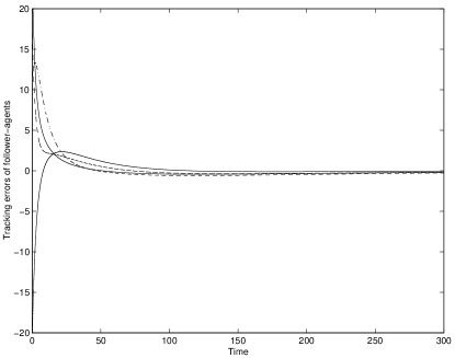
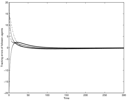
Figure 1: Position tracking errors of four followers: noise-free (on the left) and with disturbance $\delta_{i}^{j}=\sin 50t,\,i=1,...,4,j=1,2$ (on the right)

4 Conclusions

This paper discussed a group of mobile agents with an active leader moving with an unknown velocity. A neighbor-based observer design approach was proposed, along with a dynamic coordination rule developed for each autonomous agent. It was proved that this distributed control guarantees the leader-following in a switching network topology. Moreover, the tracking error has been evaluated, even in a noisy environment.

This work was supported in part by the NNSF of China under Grants 60425307, 10472129, 50595411, and 60221301, and in part by the US NSF Grant No. ECS-0322618 and Grant No. ECS-0621605.

References

Fax, A., & Murray, R. M. (2004). Information flow and cooperative control of vehicle formations, IEEE Trans. on Automatic Control, 49(9), 1465-1476, .

Godsil C. & Royle, G. (2001). Algebraic Graph Theory, New York: Springer-Verlag.

Hong, Y., Gao, L., Cheng, D., & Hu, J. (2007). Lyapunov-based approach to multi-agent systems with switching jointly-connected interconnection, IEEE Trans. Automatic Control, 52(5), 943-948.

Hong, Y., Hu, J., & Gao, L. (2006). Tracking control for multi-agent consensus with an active leader and variable topology, Automatica, 42(7), 1177-1182.

Horn, R., & Johnson, C. (1985). Matrix Analysis, New York: Cambbridge Univ. Press.

Kang, W., Xi, N., & Sparks, A. (2000). Formation control of autonomous agents in 3D workspace, Proc. of IEEE Int. Conf. on Robotics and Automation, 1755-1760, San Francisco, CA.

Lin, Z., Broucke, M., & Francis, B. (2004). Local control strategies for groups of mobile autonomous agents, IEEE Trans. Automatic Control, 49(4), 622-629.

Okubo, A. (1986). Dynamical aspects of animal grouping: swarms, schools, flocks and herds, Advances in Biophysics, 22, 1-94.

Olfati-Saber, R. (2006). Flocking for multi-agent dynamic systems: algorithms and theory, IEEE Trans. on Automatic Control, 51(3): 410-420.

Ren, W., & Beard, R. (2005). Consensus seeking in multi-agent systems using dynamically changing interaction topologies, IEEE Trans. Automatic Control, 50(4), 665-671.

Shi, H., Wang, L., & Chu, T. (2006). Virtual leader approach to coordinated control of multiple mobile agents with asymmetric interactions, Physica D, 213, 51-65.

Hong, Y., Chen, G., & Bushnell, L. (2008). Distributed observers design for leader-following control of multi-agent networks, Automatica, 44 (3), 846-850.

Wang, X.,& Hong, Y. (2009). Distributed observers for tracking a moving target by cooperative multiple agents with time delays, Proc. of ICCAS-SICE 2009, 982-987, Japan.