Limitation of SDMA in Ultra-Dense Small Cell Networks

Abstract

Benefitting from multi-user gain brought by multi-antenna techniques, space division multiple access (SDMA) is capable of significantly enhancing spatial throughput (ST) in wireless networks. Nevertheless, we show in this letter that, even when SDMA is applied, ST would diminish to be zero in ultra-dense networks (UDN), where small cell base stations (BSs) are fully densified. More importantly, we compare the performance of SDMA, single-user beamforming (SU-BF) (one user is served in each cell) and full SDMA (the number of served users equals the number of equipped antennas). Surprisingly, it is shown that SU-BF achieves the highest ST and critical density, beyond which ST starts to degrade, in UDN. The results in this work could shed light on the fundamental limitation of SDMA in UDN.

I Introduction

While network densification is promising to improve network capacity, its limitation has been manifest in recent research [1, 2, 3]. Depending on practical system settings, it is shown that area spectral efficiency would decrease as base station (BS) density grows in downlink cellular networks [2]. Worsestill, network capacity is shown to diminish to zero when single-antenna BSs are over deployed [3]. To rejuvenate the potential of network densification, space division multiple access (SDMA), which is capable of simultaneously serving multiple users within one cell over identical spectrum resources, is shown to be of great potential [4, 5]. Especially, it is shown that single-user beamforming (SU-BF), a special case of SDMA, could improve network capacity by tens of folds in ultra-dense networks (UDN), compared to the single-antenna regime [5]. However, only single user could be served within one cell using SU-BF. Therefore, it is imperative to study whether the multi-user gain of SDMA could be harvested to further improve network capacity in UDN.

In this work, we investigate the performance of SDMA in ultra-dense downlink small cell networks. As more than one user is served within one cell using SDMA, spatial resources could be fully exploited. However, it is unexpectedly shown that network spatial throughput (ST) would monotonously decrease with the number of served users within one cell when BS density is sufficiently large, which radically contradicts with the sparse deployment cases. Moreover, it is proved that applying SU-BF could as well maximize the critical density, beyond which network capacity starts to diminish. Therefore, the results reveal the fundamental limits of SDMA and confirm the superiority of SU-BF in UDN.

II System Model

We consider a downlink small cell network, where the locations of $N_{\mathrm{a}}$-antenna BSs (with constant transmit power $P$) and single-antenna users in a two-dimension plane are modeled as two independent homogeneous Poisson Point Processes (PPPs) $\Pi_{\mathrm{BS}}=\left\{\mathrm{BS}_{i}\right\}$ $\left(i\in\mathbb{N}\right)$ of density $\lambda$ and $\Pi_{\mathrm{U}}=\left\{\mathrm{U}_{j}\right\}$ $\left(j\in\mathbb{N}\right)$ of density $\lambda_{\mathrm{U}}$, respectively. If $r$ is the 2-dimension distance of cellular link, the distance between the antennas of BSs and the associated users is $d=\sqrt{r^{2}+\Delta h^{2}}$, where $\Delta h>0$ denotes the antenna height difference (AHD) between BSs and users

We further assume that each user connects to the BS providing the smallest pathloss. Accordingly, the probability density function (PDF) of $r$ is given by [6]

$$f_{r}\left(x\right)= 2\pi\lambda xe^{-\pi\lambda x^{2}}.\>\left(x\geq 0\right)$$ (1)

Denote $N_{\mathrm{U}}$ $\left(N_{\mathrm{U}}\leq N_{\mathrm{a}}\right)$ as the number of active users within one cell. Meanwhile, a dense user deployment is considered, i.e., $\lambda\gg\lambda_{\mathrm{U}}$, such that each full-buffer BS could select at most $N_{\mathrm{a}}$ users to serve using SDMA.

Channel gain consists of a pathloss component and a small-scale fading component. In particular, given transmission distance $d$, a generalized multi-slope pathloss model (MSPM) is adopted to characterize differentiated signal power attenuation rates within different regions, i.e.,

$$l_{N}\left(\left\{\alpha_{n}\right\}_{n=0}^{N-1};d\right)=K_{n}d^{-\alpha_{n}},\>R_{n}\leq d<R_{n+1}$$ (2)

where $\alpha_{n}$ denotes the pathloss exponent, $K_{0}=1$, $K_{n}=\prod_{i=1}^{n}R_{i}^{\alpha_{i}-\alpha_{i-1}}$ $\left(n\geq 1\right)$, and $0=R_{0}<R_{1}<\cdots<R_{N}=\infty$. Note that $\alpha_{i}\leq\alpha_{j}$ $\left(i<j\right)$ and $\alpha_{N-1}>2$ for practical concerns. Rayleigh fading is used to model small-scale fading for mathematical tractability. The rationality of Rayleigh fading assumption in UDN has been verified via experimental results in [7].

SDMA with zero-forcing precoding is applied, where perfect channel state information (CSI) from the BSs to the serving downlink users could be obtained to design the precoders. According to [4, 8, 9], under Rayleigh fading channels, the channel power gain caused by small-scaling fading of both direct link and interfering link follows gamma distribution when zero-forcing precoding is applied by the multi-antenna technique. If denoting $H_{\mathrm{U}_{0},\mathrm{BS}_{0}}$ as the channel power gain caused by small-scale fading from $\mathrm{BS}_{0}$ to $\mathrm{U}_{0}$ (typical pair) and $H_{\mathrm{U}_{0},\mathrm{BS}_{i}}$ $\left(i\neq 0\right)$ as the channel power gain caused by small scaling fading from $\mathrm{BS}_{i}$ (interfering BS) to $\mathrm{U}_{0}$, then $H_{\mathrm{U}_{0},\mathrm{BS}_{0}}\sim\Gamma\left(N_{\mathrm{a}}-N_{\mathrm{U}}+1,1\right)$ and $H_{\mathrm{U}_{0},\mathrm{BS}_{i}}\sim\Gamma\left(N_{\mathrm{U}},1\right)$. It is worth noting that SDMA degenerates into full SDMA when $N_{\mathrm{U}}=N_{\mathrm{a}}$, while degenerates into SU-BF when $N_{\mathrm{U}}=1$.

We use network ST for performance evaluation of SDMA in UDN. In particular, ST is defined by

$$\mathsf{ST}_{N}\left(\lambda\right)=N_{\mathrm{U}}\lambda\mathsf{CP}_{N}\left(\lambda\right)\log_{2}\left(1+\tau\right).$$ (3)

In (3), $\tau$ denotes the decoding threshold and $\mathsf{CP}_{N}\left(\lambda\right)$ denotes the coverage probability (CP) of the typical downlink users, which is given by

$$\mathsf{CP}_{N}\left(\lambda\right)=\mathbb{P}\left\{\mathsf{SIR}_{\mathrm{U}_{0}}>\tau\right\}.$$ (4)

In (4), $\mathsf{SIR}_{\mathrm{U}_{0}}$ denotes the signal-to-interference ratio (SIR) at $\mathrm{U}_{0}$. Note that the subscript ‘$N$’ denotes the number of slopes in (2).

Notation: Denoting ${}_{2}F_{1}\left(\cdot,\cdot,\cdot,\cdot\right)$ as Gaussian hypergeometric function, we denote $\omega\left(x,y,z\right)={}_{2}F_{1}\left(x,-\frac{2}{y},1-\frac{2}{y},-z\right)$ in the remaining parts. Besides, $l_{N}\left(\left\{\alpha_{n}\right\}_{n=0}^{N-1};d\right)$ is replaced by $l_{N}\left(d\right)$ for notation simplicity.

III Performance Evaluation of SDMA in UDN

In this section, we evaluate the performance of SDMA in terms of network ST, which depends on the distribution of $\mathsf{SIR}_{\mathrm{U}_{0}}$ according to (3). In particular, $\mathsf{SIR}_{\mathrm{U}_{0}}$ is given by

$$\mathsf{SIR}_{\mathrm{U}_{0}}= PH_{\mathrm{U}_{0},\mathrm{BS}_{0}}l\left(d_{0}\right)/I_{\mathrm{IC}},$$ (5)

where $I_{\mathrm{IC}}=\underset{\tiny{\mathrm{BS}_{i}\in\tilde{\Pi}_{\mathrm{BS}}}}{\sum}PH_{\mathrm{U}_{0},\mathrm{BS}_{i}}l\left(d_{i}\right)$ is the inter-cell interference, $d_{i}$ denotes the distance between the antennas of $\mathrm{BS}_{i}$ and $\mathrm{U}_{0}$, and $H_{\mathrm{U}_{0},\mathrm{BS}_{i}}$ denotes the power gain caused by small-scale-fading from $\mathrm{BS}_{i}$ to $\mathrm{U}_{0}$. Following $\mathsf{SIR}_{\mathrm{U}_{0}}$ in (5), we present the results on CP and ST in the following corollary.

Corollary 1 (CP and ST in SDMA System).

When SDMA is applied under MSPM, ST in downlink small cell networks is given by $\mathsf{ST}_{N}\left(\lambda\right)=N_{\mathrm{U}}\lambda\mathsf{CP}_{N}\left(\lambda\right)\log_{2}\left(1+\tau\right)$, where

$$\mathsf{CP}_{N}\left(\lambda\right)= \mathbb{E}\left[\stackrel{{\scriptstyle[}}{{k}}=0]{N_{\mathrm{a}}-N_{\mathrm{U}}}{\sum}\frac{\left(-s\right)^{k}}{k!}\frac{\mathrm{d}^{k}}{\mathrm{d}s^{k}}\mathcal{L}_{I_{\mathrm{IC}}}\left(s\right)\left|{}_{s=\frac{\tau}{Pl_{N}\left(d_{0}\right)}}\right.\right].$$ (6)

In (6), $\mathcal{L}_{I_{\mathrm{IC}}}\left(s\right)$ is the Laplace Transform of $I_{\mathrm{IC}}$ evaluated at $s=\frac{\tau}{Pl_{N}\left(d_{0}\right)}$, which is given by

$$\mathcal{L}_{I_{\mathrm{IC}}}\left(s\right)= e^{-2\pi\lambda\int_{d_{0}}^{\infty}x\left(1-\left(1+sPl_{N}\left(x\right)\right)^{-1}\right)\mathrm{d}x}.$$ (7)

Proof.

Following [5, Corollary 2], the results can be obtained with easy manipulation. The detail is omitted due to space limitation.∎

Corollary 1 provides a numerical approach to evaluate the performance of SDMA in UDN. As well, the impact of key parameters of SDMA, such as the number of antennas and served users, on system performance could be captured. In particular, we plot ST as a function of BS density in Fig. 1 under single-slope pathloss model (SSPM), i.e., $N=1$ in (2), and dual-slope pathloss model (DSPM), i.e., $N=2$ in (2). It can be seen from Fig. 1a that network ST could be significantly improved by SDMA, compared to the single-antenna regime. Especially, the maximal ST could be improved by 21 folds under DSPM when 16 antennas are equipped by each BS and 2 users are served within one cell. Meanwhile, we evaluate the impact of AHD on the network ST in Fig. 1b. It is observed that network ST would be significantly over-estimated without considering the AHD, i.e., ST even linearly increases with BS density. As the $\Delta h=0$m assumption is no longer impractical when the distance from transmitters and the intended receivers is small, this confirms the importance of modeling AHD when evaluating the performance of UDN.

Taking $\Delta h>0$m into account, however, it is pessimistic to observe that ST would asymptotically approach zero under dense deployment even when SDMA is applied. Therefore, we analytically study ST scaling law next.

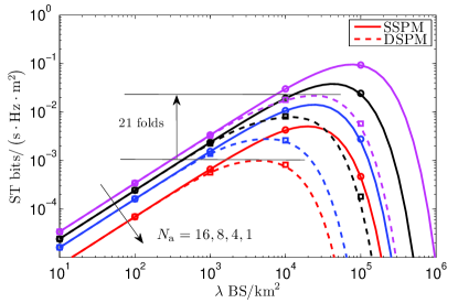
(a) Impact of $N_{\mathrm{a}}$.

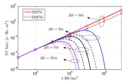
(b) Impact of AHD $\Delta h$.

Figure 1: ST scaling laws. Set $N_{\mathrm{U}}=1$ when $N_{\mathrm{a}}=1$, while set $N_{\mathrm{U}}=2$ when $N_{\mathrm{a}}>1$. For system settings, set $P=23$dBm and $\tau=10$dB. Set $\alpha_{0}=4$ for SSPM, and $\alpha_{0}=2.5$, $\alpha_{1}=4$ and $R_{1}=10$m for DSPM. In (a), set $\Delta h=2$m. In (b), set $N_{\mathrm{a}}$=16. Lines and markers denote numerical and simulation results, respectively.

Corollary 2 (CP and ST Scaling Laws in SDMA System).

In SDMA system, CP and ST scale with BS density $\lambda$ as $\mathsf{CP}_{N}\left(\lambda\right)\sim e^{-\kappa\lambda}$ and $\mathsf{ST}_{N}\left(\lambda\right)\sim\lambda e^{-\kappa\lambda}$ ($\kappa$ is a constant), respectively.

Proof.

Given the number of antennas, the experience of single user would be degraded if more users within one cell share the antenna resources. Therefore, we have $\mathsf{CP}_{N}^{\mathrm{F}}\left(\lambda\right)\leq\mathsf{CP}_{N}\left(\lambda\right)\leq\mathsf{CP}_{N}^{\mathrm{S}}\left(\lambda\right)$, where $\mathsf{CP}_{N}^{\mathrm{F}}\left(\lambda\right)$ is obtained by setting $N_{\mathrm{U}}=N_{\mathrm{a}}$ (full SDMA) and $\mathsf{CP}_{N}^{\mathrm{S}}\left(\lambda\right)$ is obtained by setting $N_{\mathrm{U}}=1$ (SU-BF). Hence, $\mathsf{CP}^{\mathrm{F}}\left(\lambda\right)$

$$\overset{\left(\mathrm{a}\right)}{=} \mathbb{E}_{r_{0}}\left[\exp\left(-2\pi\lambda\int_{d_{0}}^{\infty}x\left(1-\left(1+sPl_{N}\left(x\right)\right)^{-N_{\mathrm{a}}}\right)\mathrm{d}x\right)\right]$$

$$> \mathbb{E}_{r_{0}>R_{N-1}}\left[\exp\left(-2\pi\lambda\int_{d_{0}}^{\infty}x\left(1-\left(1+sPl_{N}\left(x\right)\right)^{-N_{\mathrm{a}}}\right)\mathrm{d}x\right)\right]$$

$$\overset{\left(\mathrm{b}\right)}{=} \mathbb{E}_{r_{0}>R_{N-1}}\left[\exp\left(-\pi\lambda d_{0}^{2}\left(\omega\left(N_{\mathrm{a}},\alpha_{N-1},\tau\right)-1\right)\right)\right]$$

$$\overset{\left(\mathrm{c}\right)}{=} \frac{\exp\left[-\pi\lambda\left(\omega\left(N_{\mathrm{a}},\alpha_{N-1},\tau\right)\left(R_{N-1}^{2}+\Delta h^{2}\right)-\Delta h^{2}\right)\right]}{\omega\left(N_{\mathrm{a}},\alpha_{N-1},\tau\right)}$$

$$= \mathsf{CP}_{N}^{\mathrm{L}}\left(\lambda\right),$$ (8)

where $s=\frac{\tau}{Pl_{N}\left(d_{0}\right)}$. In (8), (a) follows due to $H_{\mathrm{U}_{0},\mathrm{BS}_{0}}\sim\Gamma\left(1,1\right)$ since $N_{\mathrm{a}}=N_{\mathrm{U}}$, (b) follows due to $s=\frac{\tau}{PK_{N-1}d_{0}^{-\alpha_{N-1}}}$ and $l_{N}\left(x\right)=K_{N-1}x^{-\alpha_{N-1}}$ when $r_{0}>R_{N-1}$, and (c) follows due to the PDF of $r_{0}$ given in (1). In consequence, $\mathsf{CP}_{N}^{\mathrm{L}}\left(\lambda\right)\sim e^{-\kappa\lambda}$ holds. Besides, it follows from [5, Theorem 2] that $\mathsf{CP}^{\mathrm{S}}\left(\lambda\right)\sim e^{-\kappa\lambda}$. Therefore, $\mathsf{CP}_{N}\left(\lambda\right)\sim e^{-\kappa\lambda}$.

Following the definition of ST, the proof is complete.∎

Corollary 2 reveals the fundamental limitation of SDMA in UDN. Meanwhile, it is intuitive to obtain that SU-BF outperforms SDMA and full SDMA in terms of CP. Therefore, it is interesting to analytically compare the performance of these schemes in terms of ST as well, the detail of which is presented in the following part.

IV SDMA, Full SDMA and SU-BF: A Special Case Study

In this section, analytical comparison of SDMA, full SDMA and SU-BF is made from the ST perspective. Especially, a special case study is performed under SSPM given by

$$l_{1}\left(d\right) =d^{-\alpha_{0}}.\>d\geq 0$$ (9)

Nevertheless, the results on ST in Corollary 1 are much too complicated even when SSPM is applied. To facilitate the comparison, we first present a simple but effective approximation on ST in the Proposition 1.

Proposition 1.

When SDMA is applied under SSPM, ST in ultra-dense downlink small cell networks can be approximated as $\mathsf{ST}_{1}^{\dagger}\left(\lambda\right)=\lambda\mathsf{CP}_{1}^{\dagger}\left(\lambda\right)\log_{2}\left(1+\tau\right)$, where

$$\mathsf{CP}_{1}^{\dagger}\left(\lambda\right)= \frac{\exp\left(-\pi\lambda\delta\left(\alpha_{0}\right)\right)}{\omega\left(N_{\mathrm{U}},\alpha_{0},\tau^{\mathrm{S}}\right)},$$ (10)

where $\delta\left(x\right)=\Delta h^{2}\left(\omega\left(N_{\mathrm{U}},x,\tau^{\mathrm{S}}\right)-1\right)$ and $\tau^{\mathrm{S}}=\frac{\tau}{N_{\mathrm{a}}-N_{\mathrm{U}}+1}$.

Proof.

The key to the approximation is to use $G_{\mathrm{U}_{0},\mathrm{BS}_{0}}\sim\mathrm{Exp}\left(\frac{1}{N_{\mathrm{a}}-N_{\mathrm{U}}+1}\right)$ to replace $H_{\mathrm{U}_{0},\mathrm{BS}_{0}}\sim\varGamma\left(N_{\mathrm{a}}-N_{\mathrm{U}}+1,1\right)$. Accordingly, we have

$$\mathsf{CP}_{1}^{\dagger}\left(\lambda\right)= \mathbb{E}_{r_{0}}\left[e^{-2\pi\lambda\int_{d_{0}}^{\infty}x\left(1-\left(1+s^{\dagger}Pl_{1}\left(x\right)\right)^{-N_{\mathrm{U}}}\right)\mathrm{d}x}\right]$$

$$= \mathbb{E}_{r_{0}}\left[e^{-\pi\lambda d_{0}^{2}\left[\omega\left(N_{\mathrm{U}},\alpha_{0},\tau^{\mathrm{S}}\right)-1\right]}\right],$$ (11)

where $s^{\dagger}=\frac{\tau^{\mathrm{S}}}{Pl_{1}\left(d_{0}\right)}$ and $d_{0}=\sqrt{r_{0}^{2}+\Delta h^{2}}$. Aided by (11) and the PDF of $r_{0}$ given in (1), $\mathsf{CP}_{1}\left(\lambda\right)$ can be obtained.∎

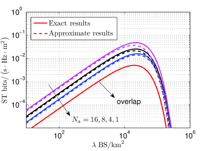
(a) Examine the approximation accuracy.

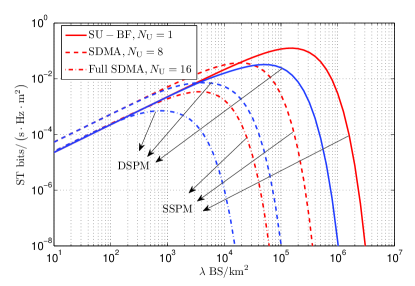
(b) Comparison of SDMA, full SDMA and SU-BF.

Figure 2: ST scaling laws. In (a), set $N_{\mathrm{U}}=1$ when $N_{\mathrm{a}}=1$ and set $N_{\mathrm{U}}=N_{\mathrm{a}}/2$ when $N_{\mathrm{a}}>1$. In (b), set $N_{\mathrm{a}}$=16 and other system parameters are identical to those in Fig. 1.

We next verify the accuracy of the approximation in Proposition 1 using Fig. 2a. It can be seen that the gaps between the exact and approximate results are small. They even overlap when $N_{\mathrm{a}}=1$. Moreover, it is observed that the critical densities obtained via the approximate and exact results are almost identical. Therefore, it is valid to use the approximate results to derive critical density as follows.

Corollary 3.

The critical density in SDMA downlink small cell networks is given by

$$\lambda^{*}= \frac{1}{\pi\Delta h^{2}\left(\omega\left(N_{\mathrm{U}},\alpha_{0},\tau^{\mathrm{S}}\right)-1\right)},$$ (12)

where $\tau^{\mathrm{S}}=\frac{\tau}{N_{\mathrm{a}}-N_{\mathrm{U}}+1}$.

Proof.

The proof can be feasibly completed by solving $\frac{\partial\mathsf{ST}_{1}^{\dagger}\left(\lambda\right)}{\partial\lambda}=0$.∎

Corollary 3 identifies the relationship of key system parameters and critical density. For instance, it is apparent that $\lambda^{*}$ inversely increases with $\Delta h^{2}$. For this reason, it is suggested to lower the transmitter and receiver antenna heights and reduce the AHD such that network densification could be still effective in enhancing spectrum efficiency even when BS density is large.

Next, we use the results in Corollary 3 to further evaluate the performance of SDMA, full SDMA and SU-BF in UDN. Before that, the results on $\omega\left(x,y,z\right)$ are given in Lemma 1.

Lemma 1.

Given $N>1$ (an integer), $-1<b<0$, $c>0$ and $z<0$, ${}_{2}F_{1}\left(N,b,c,z\right)$ is an increasing function of $N$.

Proof.

The proof can be completed using mathematical induction. Assuming $\varDelta_{1}={}_{2}F_{1}\left(N+1,b,c,z\right)-{}_{2}F_{1}\left(N,b,c,z\right)=\frac{bz}{c}{}_{2}F_{1}\left(N+1,b+1,c+1,z\right)>0$, if the inequality $\varDelta_{2}={}_{2}F_{1}\left(N+2,b,c,z\right)-{}_{2}F_{1}\left(N+1,b,c,z\right)>0$ holds, the proof is complete. By definition of hypergemetric function, we have

$$\varDelta_{2} =\frac{bz}{c}{}_{2}F_{1}\left(N+2,b+1,c+1,z\right)$$

$$=\frac{b}{N+1}\left[{}_{2}F_{1}\left(N+1,b+1,c,z\right)-{}_{2}F_{1}\left(N+1,b,c,z\right)\right].$$ (13)

As $N>0$ and $b<0$, to prove $\varDelta_{2}>0$, it is sufficient to show ${}_{2}F_{1}\left(N,b+1,c,z\right)-{}_{2}F_{1}\left(N,b,c,z\right)<0$. Hence, we have

$$\varDelta_{3}= {}_{2}F_{1}\left(b+1,N,c,z\right)-{}_{2}F_{1}\left(b,N,c,z\right)$$

$$= \frac{Nz}{c}{}_{2}F_{1}\left(b+1,N+1,c+1,z\right)$$

$$= \frac{Nz}{c}{}_{2}F_{1}\left(N+1,b+1,c+1,z\right).$$ (14)

According to the assumption that $\varDelta_{1}>0$, we have ${}_{2}F_{1}\left(N+1,b+1,c+1,z\right)>0$. Therefore, $\varDelta_{3}<0$ holds.∎

Aided by Lemma 1, we provide the results on full SDMA in the following theorem.

Theorem 1.

When full SDMA is applied, the critical density of downlink small cell networks is a decreasing function of the number of antennas.

Proof.

Applying full SDMA, $N_{\mathrm{U}}=N_{\mathrm{a}}$ and the critical density in Corollary 3 degenerates into

$$\lambda^{*}= \frac{1}{\pi\Delta h^{2}\left(\omega\left(N_{\mathrm{a}},\alpha_{0},\tau\right)-1\right)}.$$ (15)

Since $\omega\left(N_{\mathrm{a}},\alpha_{0},\tau\right)$ is an increasing function of $N_{\mathrm{a}}$ (Lemma 1), the proof is complete.∎

Theorem 1 evaluates the performance of full SDMA in terms of critical density. More specifically, it is observed from Fig. 2b that ST would begin to decrease at a smaller critical density when more antennas are equipped. Following Theorem 1, we further compare SDMA, full SDMA and SU-BF in Theorem 2.

Theorem 2.

Given the number of antennas equipped on each BS, the critical density achieved by SU-BF is greater than those achieved by SDMA and full SDMA.

Proof.

The results can be proved by showing $\lambda^{*}$ in Corollary 3 is a decreasing function of $N_{\mathrm{U}}$ or equivalently $\omega\left(N_{\mathrm{U}},\alpha_{0},\tau^{\mathrm{S}}\right)$ is an increasing function of $N_{\mathrm{U}}$. By making an extension of [3, Lemma 1], it can be shown that $\omega\left(N_{\mathrm{U}},\alpha_{0},\tau^{\mathrm{S}}\right)$ increases with $\tau^{\mathrm{S}}=\frac{1}{N_{\mathrm{a}}-N_{\mathrm{U}}+1}$, which monotonously increases with $N_{\mathrm{U}}$. Therefore, aided by Lemma 1, it can be proved that $\omega\left(N_{\mathrm{U}},\alpha_{0},\tau^{\mathrm{S}}\right)$ increases with $N_{\mathrm{U}}$.∎

Theorem 2 indicates that simultaneously serving multiple users would enable ST to decrease at a smaller BS density. In other words, compared to SU-BF, SDMA potentially degrades spectrum efficiency in UDN. This is inconsistent with traditional understanding of SDMA in sparse deployment [4], which shows higher spectrum efficiency could be achieved by SDMA via serving more users. This can be verified via the results in Fig. 2b. Specifically, although a higher ST could be obtained by SDMA when $N_{\mathrm{U}}$ is large in sparse scenario, it would experience a notable decrease at a greater BS density, compared to SU-BF. The intuition behind this is that the multi-user gain harvested by SDMA is ruined by the overwhelming interference in UDN.

Besides, it is numerically shown in Fig. 2b that SU-BF outperforms SDMA and full SDMA in terms of ST in UDN as well. From this perspective, SU-BF is more favorable to enhance network capacity in UDN. While the analytical comparison is made based on SSPM, it could be easily tested that the comparison results are still valid under MSPM. For instance, the results under DSPM, i.e., $N=2$ in (2), are verified in Fig. 2b.

V Conclusion

In this letter, the performance of SDMA has been explored in ultra-dense downlink small cell networks. Specifically, SDMA, albeit incapable of improving network capacity scaling law, is proved to significantly enhancing spatial throughput, compared to single-antenna regime. Moreover, it is interestingly shown that network capacity and critical density could be maximized when single user is served in each small cell, which contradicts with the intuition. The primary reason is that demerits of overwhelming inter-cell interference dominate the benefits of multi-user gain of SDMA in UDN. Therefore, the outcomes of this work could provide guideline towards the application and optimization of SDMA in UDN via reasonably selecting the number of users to serve.

References

• [1] X.Β Zhang and J.Β G. Andrews, β€œDownlink cellular network analysis with multi-slope path loss models,” IEEE Trans. Commun., vol.Β 63, no.Β 5, pp. 1881–1894, May. 2015.
• [2] M.Β D. Renzo, W.Β Lu, and P.Β Guan, β€œThe intensity matching approach: A tractable stochastic geometry approximation to system-level analysis of cellular networks,” IEEE Trans. Wireless Commun., vol.Β 15, no.Β 9, pp. 5963–5983, Sep. 2016.
• [3] J.Β Liu, M.Β Sheng, L.Β Liu, and J.Β Li, β€œEffect of densification on cellular network performance with bounded pathloss model,” IEEE Commun. Lett., vol.Β 21, no.Β 2, pp. 346–349, Feb. 2017.
• [4] H.Β S. Dhillon, M.Β Kountouris, and J.Β G. Andrews, β€œDownlink MIMO hetnets: Modeling, ordering results and performance analysis,” IEEE Trans. Wireless Commun., vol.Β 12, no.Β 10, pp. 5208–5222, Oct. 2013.
• [5] J.Β Liu, M.Β Sheng, and J.Β Li, β€œMISO in ultra-dense networks: Balancing the tradeoff between user and system performance,” submitted to IEEE Trans. Wireless Commun., 2017. [Online]. Available: https://arxiv.org/abs/1707.05957
• [6] D.Β Stoyan, W.Β S. Kendall, J.Β Mecke, and L.Β Ruschendorf, Stochastic geometry and its applications.Β Β Β Wiley Chichester, 1995, vol.Β 2.
• [7] J.Β Liu, M.Β Sheng, L.Β Liu, and J.Β Li, β€œNetwork densification in 5G: From the short-range communications perspective,” vol. abs/1606.04749, 2017. [Online]. Available: http://arxiv.org/abs/1606.04749
• [8] N.Β Jindal, J.Β G. Andrews, and S.Β Weber, β€œMulti-antenna communication in ad hoc networks: Achieving MIMO gains with SIMO transmission,” IEEE Trans. Commun., vol.Β 59, no.Β 2, pp. 529–540, Feb. 2011.
• [9] R.Β W.Β H. Jr, T.Β Wu, Y.Β H. Kwon, and A.Β C.Β K. Soong, β€œMultiuser MIMO in distributed antenna systems with out-of-cell interference,” IEEE Trans. Signal Process., vol.Β 59, no.Β 10, pp. 4885–4899, Oct 2011.