Emotion-Based Crowd Simulation Model Based on Physical Strength Consumption for Emergency Scenarios

Abstract

Increasing attention is being given to the modeling and simulation of traffic flow and crowd movement, two phenomena that both deal with interactions between pedestrians and cars in many situations. In particular, crowd simulation is important for understanding mobility and transportation patterns. In this paper, we propose an emotion-based crowd simulation model integrating physical strength consumption. Inspired by the theory of “the devoted actor,” the movements of each individual in our model are determined by modeling the influence of physical strength consumption and the emotion of panic. In particular, human physical strength consumption is computed using a physics-based numerical method. Inspired by the James-Lange theory, panic levels are estimated by means of an enhanced emotional contagion model that leverages the inherent relationship between physical strength consumption and panic. To the best of our knowledge, our model is the first method integrating physical strength consumption into an emotion-based crowd simulation model by exploiting the relationship between physical strength consumption and emotion. We highlight the performance on different scenarios and compare the resulting behaviors with real-world video sequences. Our approach can reliably predict changes in physical strength consumption and panic levels of individuals in an emergency situation.

1 Introduction

Efficient and accurate crowd simulation is useful for intelligent transportation systems since it can help improve emergency planning and prevent congestion in transit hubs such as train stations and airports [1]. One can also analyze human mobility through the trajectories obtained by crowd simulation models to get more knowledge of pedestrian mobility behaviors in both qualitative and quantitative ways. Because of various complex factors, it is challenging to model realistic crowd behaviors in emergency scenarios. At a broad level, crowd behavior in emergencies is governed by panic and physical strength consumption [2].

The main purpose of crowd simulation algorithms is to model the movements (in terms of speed and direction) of individuals in a crowd [3]. We basically deal with two aspects of human motivations: physiological and psychological factors. Physical strength consumption and emotion [4] are two representative physiological and psychological factors, respectively. Both have a great influence on individual movements. These two factors influence each other and evolve dynamically. It is important to describe the inherent relationship between these two factors, which is more obvious in emergency or evacuation situations [5]. Many approaches incorporate emotions of individuals in crowd simulations, making it one of the most commonly used psychological factors [6]. Panic can prevent an individual from taking proper actions in emergency situations [4]. Researchers have observed that external dangers can directly cause changes in panic levels in an individual, thereby further determining his or her movements [7]. We mainly focus on the emotion of panic in emergency situations. Most of the previous studies don’t consider the effect of physical strength consumption on panic [8]. Physical strength is a person’s or animal’s ability to exert force on physical objects using muscles [9]. Physical strength consumption is defined as the energy expenditure [10] of a human, which directly affects that human’s moving speed [11]. However, it is difficult to describe the inherent relationship between physical strength consumption and panic and to then combine these factors to determine the movement of each individual [5]. Therefore, an emotion-based crowd simulation model integrating physical strength consumption is challenging due to the following reasons:

(1) It is difficult to model the physical strength consumption of an individual in a crowd accurately [12]. This task involves considering many factors that are needed to quantify the influence of physical strength consumption on crowd movement [13].

(2) Accurately modeling an individual’s panic level in a crowd is difficult because of its constant and dynamic changes [14]. Various factors such as physical strength consumption and individual movement affect panic levels.

Inspired by the theory of “the devoted actor” [2], which shows that an individual’s physiological state has an effect on his or her psychological state, we propose the first (to the best of our knowledge) emotion-based crowd simulation model based on physical strength consumption (illustrated in Figure 1). The main contributions of our work include:

• We introduce a physical strength consumption calculation method based on how individuals work under the laws of physics and quantitively characterize their dynamic changes during the crowd movement.

• We present a comprehensive emotion calculation method for physical strength consumption based on the James-Lange theory. Our new proposed model is used to derive the relationship between physical strength consumption and panic and examines how both of them govern the movement.

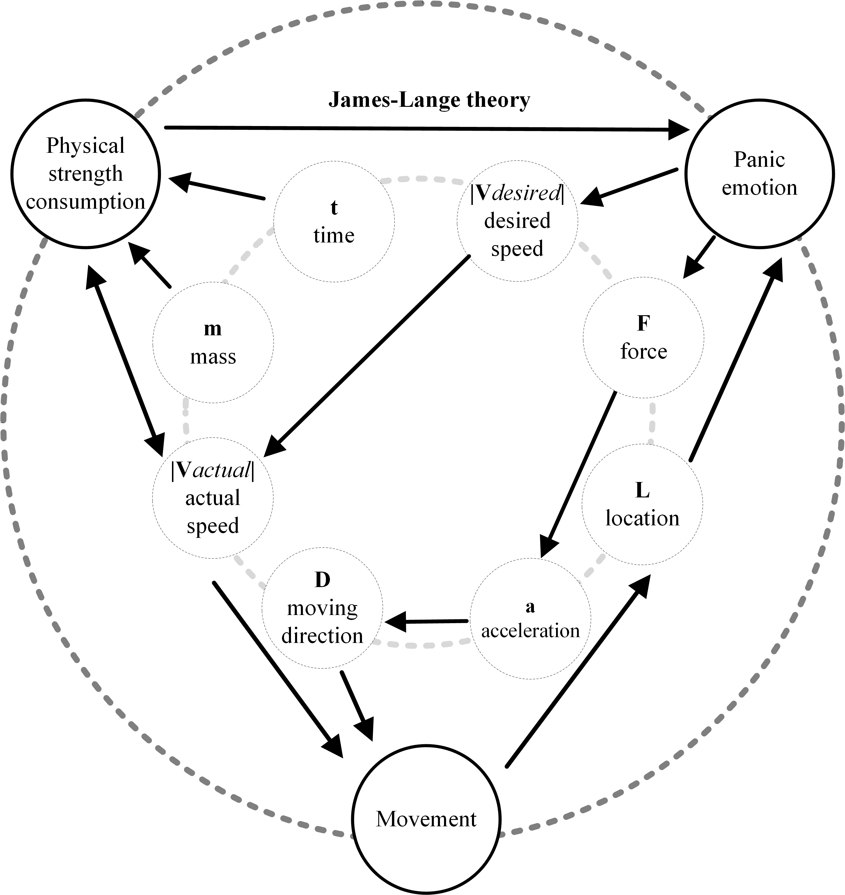
Figure 1: The relationships among physical strength consumption, panic, and movement of individuals in a crowd. Physical strength consumption is calculated according to the actual speed, mass, and moving time of individuals. The panic levels are determined by the location and physical strength consumption of the individual, and they further affect the individual’s desired speed. Moreover, each individual’s current panic level will affect his or her moving direction by changing the acceleration based on the inferred force.

The rest of this paper is organized as follows. Background and related work are reviewed in Section 2. The definition of our proposed crowd simulation model is introduced in Section 3. Different benchmark scenarios and results are presented in Section 4.

2 Related Work

In this section, we provide a brief overview of prior work on crowd simulation. We divide the summaries based on whether the works involve physical, psychological, or physiological factors.

2.1 Simple crowd simulation models

In this subsection, we summarize representative crowd simulation models that do not consider psychological or physiological factors [15, 16, 17, 1].

In the real world, many environmental factors influence an individual’s movement, i.e. scene layout, moving pedestrians, and stationary groups [18, 19, 20]. During the evacuation of a crowd, the behavioral choice of an individual is highly dependent on the moving directions of nearby individuals, the hazard location, and obstacles [21]. Moussaid et al. [22] propose a cognitive science approach based on behavioral heuristics. Guided by visual information, pedestrians apply two simple cognitive procedures to adapt their moving directions and speed. Zhou et al. [23] propose a fuzzy logic approach to model and simulate pedestrian dynamic behaviors, which are based on human experiences and human knowledge, and perceptual information obtained from interactions with the surrounding environment. Zhou et al. [24] focus on the role of leaders who can guide the movements of passengers during the evacuation. Cassol et al. [25] focus on global path planning with the main goal of identifying the best evacuation routes for a specific population when leaving a certain building. To realize better behavioral choices, most approaches calculate the position of each individual at the next time step to obtain a conflict-free moving path in a global scenario [26]. However, these approaches are not applicable to highly complex scenes with dense crowds. Other approaches use local obstacle avoidance methods. Namely, once the movement state of an individual is determined, the movement states of other individuals are updated by using local collision avoidance techniques [27].

In practice, these approaches face many difficulties in terms of accurately controlling the individual movements. Researchers in this field are increasingly focusing on integrating global path planning and local obstacle avoidance [28, 29]. Weiss et al. [30] model collision avoidance constraints both in terms of short and long-term ranges to deal with sparse and dense crowds. In [31], intergroup- and intragroup-level techniques are presented to perform coherent and collision-free navigation using reciprocal collision avoidance. Mutual information about the dynamic crowd is used to guide agents’ movements by combining both macroscopic and microscopic controls [32]. By constructing a visual tree, the shortest path without collisions is obtained in [33]. In addition, in [34, 35, 36], and [37], path planning and navigation algorithms are described for crowd simulation in complex contexts. Furthermore, in [38], an effective long-range collision avoidance algorithm is proposed.

In contrast to these works, our model enhances the traditional social force model to avoid collisions with surrounding individuals and obstacles by combining panic and physical strength consumption calculations. Traditional crowd simulation models are not concerned with this approach. In our model, we mainly deal with moving directions and moving speeds, which are largely influenced by panic and physical strength consumption during a relatively short period of time.

2.2 Crowd simulation with psychological factors

The psychological state of an individual plays a vital role in his or her decision-making process [39, 40, 41]. Stress and panic are typical psychological factors and have a great influence on the movement of individuals in a crowd. In this subsection, we introduce representative works on them.

In [14], authors focus on stress, which is defined as any change caused by interactions between the environment and individuals. Generally, stress is caused by a discrepancy between environmental demands and the abilities of individuals. Stress can have positive effects on individual behavior. In emergency or evacuation situations, stress improves the performance of individuals [14]. It can be chronic and long-term [14]. However, stress and panic are inherently different. Panic is short-term and changeable [42] and usually leads to negative effects on individuals [43]. One of the most disastrous forms of collective human behavior is the kind of crowd stampede induced by panic, often leading to fatalities as people are crushed or trampled [7].

An individual’s stress and panic are mirrored by others and they are disseminated within the crowd [6]. There are two separate lines of emotional contagion research: epidemiological-based and thermodynamics-based.

The epidemiological SIR model [44] divides the individuals in a crowd into three categories: infected, susceptible, and recovered. At first this model is used to simulate the spread of rumor [45]. Then the epidemiological SIR model is used to describe emotion propagation. In [6], the epidemiological SIR model is combined with the OCEAN personality model [46]. The phenomenon of emotional contagion occurs more obviously in a panicked crowd. In [47], the cellular automata model is combined with the SIR model (CA-SIRS) to describe emotional contagion in an emergency situation. In [48], a qualitatively simulated approach is proposed to model emotional contagion process in a large-scale emergency evacuation siutation, which confirms that the effectiveness of rescue guidance is influenced by the leading emotion of the crowd. There is another kind of emotional contagion models based on thermodynamics [49]. Bosse et al. define emotional contagion within groups based on a multi-agent approach. They focuses mostly on emotions of groups rather than those of single individuals. Neto et al. [40] improve this model adapting it into BioCrowds and coping with emotional contagion within different groups of agents. Some researchers combine these two kinds of emotional contagion models to describe dynamic emotion propagation from the perspective of social psychology [50].

Because panic has a great influence on individual movement and often leads to serious consequences, we focus on panic in emergency situations. Inspired by the James-Lange theory in biological psychology, we improve the Durupinar model [6] by considering the influence of physical strength consumption on panic levels. In contrast to previous methods considering only panic, we further demonstrate the relationship between physical strength consumption and panic.

2.3 Crowd simulation with physiological factors

To complete a comprehensive analysis of crowd movement, we must consider not only psychological factors, but also physiological factors of individuals as other important factors in determining the crowd movement [11].

Physical strength is one of the most important physiological parameters that affects individual movement. Bruneau et al. [51] apply the principle of minimum energy (PME) on groups of different sizes and densities. In [10, 52], some physiological indicators (such as physical strength consumption and heart rate) are described. Furthermore, the relationship between physical strength consumption and heart rate is revealed, which is also a method for predicting physical strength consumption based on heart rate during moderate and vigorous exercise. Work in [11] shows that the relationship between physical strength consumption and speed is nonlinear. In [13], researchers investigate how the cumulative consumption of physical strength affects the evacuation time of individuals. Guy et al. [53] propose the principle of least effort (PLE) to compute the physical strength consumption required by various movements. Furthermore, Guy et al. [54] propose a less energy-consuming, conflict-free crowd movement method based on the criterion of minimal physical strength consumption [53]. These approaches are focused on the relationship between physical strength and other physiological parameters (heart rate and oxygen uptake, for example) or individual movement. In [12], the authors choose four other basic physiological characteristics, including gender, age, health, and body shape, and map them to a navigation method.

Inspired by prior approaches, we focus on physical strength consumption, which is a very important physiological factor. Physical strength consumption is central to research in human biology and biological anthropology [55] and is closely related to a variety of factors such as heart rate, oxygen consumption, etc. [52]. It directly affects the moving speed of an individual [13]. Other physiological factors (such as gender, age, health, and body shape) can influence movement through physical strength consumption. We analyze the relationship between physical strength consumption and panic. We also describe the effects of physical strength consumption on the physical movements of individuals.

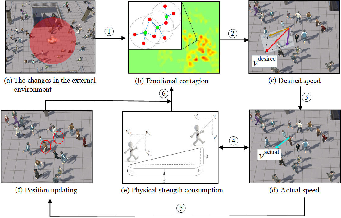
Figure 2: The flowchart of our model. (a) Changes in the external environment can cause emotional fluctuations. For example, a hazard occurs and the red area represents the range of influence of the hazard. (b) The emotional changes of one individual are calculated according to the direct impact of the hazard and emotional contagion of his or her neighbors (Section 3.3). (c) The desired speed and direction of each individual are calculated based on an updated panic assessment (Section 3.4). (d) Using the limit of physical strength consumption, the actual speed is determined [11] (Section 3.4). (e) The calculation of physical strength consumption affected by the actual speed (Section 3.2). In contrast, the cumulative physical strength consumption also determines the actual maximal speed of the individual at the next timestep (Section 3.4). The current physical strength consumption reflects the emotional experience of an individual (Section 3.3). (f) The position of the individual is updated according to its actual speed. If the individual is panicked, we return to step (b); otherwise, the flowchart ends (Section 3.3).

3 Our Model

Our emotion-based crowd simulation model comprehensively considers physical strength consumption in emergencies to influence crowd movement. The flowchart of our model is presented in Figure 2. Strenuous movements are often observed in individuals in emergency or evacuation situations, and the relationship among them is more obvious in such situations [56]. Therefore, we mainly focus on simulating crowd movements in such emergency situations.

Our model consists of three important components: physical strength consumption, panic, and individual movement. Human physical strength consumption is computed with a physics-based method (Section 3.2). Panic levels are determined through an enhanced emotional contagion model that leverages the inherent relationship between physical strength consumption and panic (Section 3.3). Our model computes the movement of an individual by modeling the physical influence of strength consumption and panic (Section 3.4).

3.1 Symbols and notations

For convenience, the important parameters and their descriptions used in our model are listed in Table I.

TABLE I: The parameters used in our model.

Notation	Description
$P\left(t\right)$	Physical strength consumption at time $t$
$P_{hor}\left(t\right)$	Physical strength consumption along the horizontal direction at time $t$
$P_{ver}\left(t\right)$	Physical strength consumption along the vertical direction at time $t$
$F^{x}$	Driving force of individual along the horizontal direction
$F^{y}$	Pulling force of individual along the vertical direction
$E$	Panic emotion
$E_{o}$	Emotional cognitive component
$E_{p}$	Emotional experience component
$E_{o}^{h}$	The emotion affected by hazards
$E_{o}^{c}$	Emotional contagion
$V_{i}\left(t\right)$	Moving direction of the individual $i$ at time $t$
$V_{i}^{s}\left(L,t\right)$	Safety evacuation direction of the individual $i$ at location $L$ and at time $t$
$V_{i}^{round}\left(t\right)$	Combined moving directions of individuals who are in the perceived range of the individual $i$ at time $t$
$v_{i}^{desired}$	The desired speed $v_{i}^{desired}$ of the individual $i$ considers only the emotion factor.
$v_{i}^{actual}$	The actual speed $v_{i}^{actual}$ of the individual $i$ is limited by his own physical strength consumption.
$v^{p}$	Maximum speed $v^{p}$ according to current physical strength consumption
$v_{i}^{\textit{MAX}}$	Maximum speed that the individual $i$ can run
$v_{i}^{\textit{NOR}}$	Speed of the individual $i$ in the normal case (emotion value is equal to zero)
PR	The radius of perceived range
Num	The number of individuals in a scene
$R_{a}$	The radius of an individual

3.2 Physical strength consumption calculation

Physical strength consumption is one of the most commonly used physiological indicators and is closely related to individual movement. It is defined by the following equation:

$$P\left(t\right)=P_{hor}\left(t\right)+P_{ver}\left(t\right)$$ (1)

where $P\left(t\right)$ denotes the total physical strength consumption at time $t$ and $P_{hor}\left(t\right)$, $P_{ver}\left(t\right)$ denote the physical strength consumption along the horizontal and the vertical directions, respectively. They are defined as follows:

$$P_{hor}\left(t\right)=\sum\limits_{i=1}^{t}{F^{x}_{i}\cdot d_{i}}$$ (2)

$$P_{ver}\left(t\right)=\sum\limits_{i=1}^{t}{F^{y}_{i}\cdot h_{i}}$$ (3)

$F^{x}_{i}$ is the driving force of the individual along the horizontal direction. This force overcomes friction. $d_{i}$ is the moving distance of the individual at time $t$. $F^{x}_{i}\cdot d_{i}$ represents the work done by the individual along the horizontal direction. $F^{y}_{i}$ is the pulling force of the individual along the vertical direction. This force overcomes gravity. $h_{i}$ is the rising height of the individual at time $t$, and $F^{y}_{i}\cdot h_{i}$ represents the work done by the individual along the vertical direction.

According to the laws of physics, $F^{x}_{i}$ is defined as follows:

$$F^{x}_{i}=f_{i}+\frac{(v_{i}^{x}-v_{i-1}^{x})m}{\tau}$$ (4)

A diagram of the physical strength consumption calculation is shown in Figure 3.

The friction $f_{i}$ is defined in Equation 5, $k_{i}$ is defined in Equation 6, and $t_{i}$ is defined in Equation 7 according to [57, 58]. $\mu$ is the friction factor, which is related to the shoes and the ground. In our implementation, $\mu$=0.58 is adopted, which is also recommended in [59]. $v_{i}$ is the current velocity magnitude, $v_{min}$ is the minimal velocity magnitude, and $v_{max}$ is the maximal velocity magnitude.

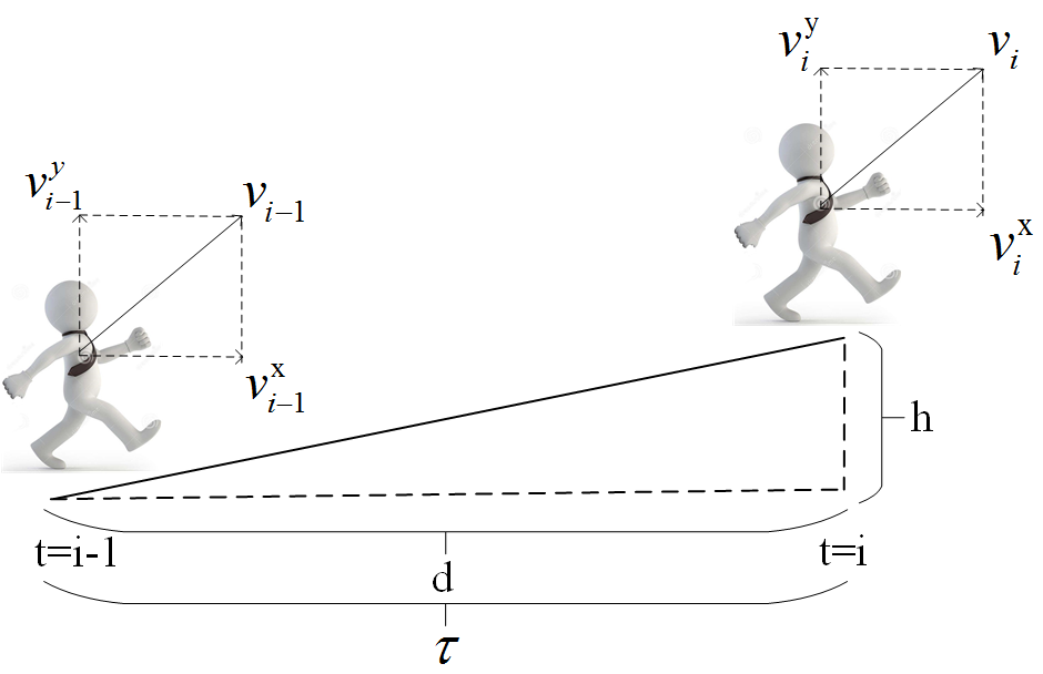
Figure 3: Schematic of the physical strength consumption calculation. $v_{i}^{x}$ is the velocity component of an individual in the horizontal direction at time $i$, and the length of each time step is $\tau$. The horizontal speed of the individual changes from $v_{i-1}^{x}$ to $v_{i}^{x}$ in time interval $\tau$.

$$f_{i}=t_{i}\cdot\mu\cdot mg\cdot k_{i}$$ (5)

$$k_{i}=1.5+0.5\cdot\frac{v_{i}-v_{min}}{v_{max}-v_{min}}$$ (6)

$$t_{i}=0.6-0.2\cdot\frac{v_{i}-v_{min}}{v_{max}-v_{min}}$$ (7)

where $k_{i}$ is the coefficient of the weight, $t_{i}$ is the time of the individual’s foot touching the ground, $k_{i}\propto v_{i}$, $t_{i}\propto^{-1}v_{i}$, $f_{i}\propto k_{i}$, and $f_{i}\propto t_{i}$. If one stands with both feet on a force plate, $t_{i}=k_{i}=1$.

The physical strength consumption in the horizontal direction is defined by:

According to the laws of physics, $F^{y}_{i}$ is defined by the following equation:

$$F^{y}_{i}=mg+\frac{(v_{i}^{y}-v_{i-1}^{y})m}{\tau}$$ (9)

where $v_{i}^{y}$ is the velocity component in the vertical direction at time $i$.

The physical strength consumption in the vertical direction is defined by:

3.3 Panic calculation considering physical strength consumption

This section presents the calculation method for the panic level of an individual. $E\in[0,1]$ indicates the approximate level of panic. The panic level $E$ consists of two components. The first is the emotional cognitive component $E_{o}$, which relates to the hazard and encompasses emotional contagion. The second is the emotional experience component $E_{p}$, which is calculated using physical strength consumption and heart rate. Therefore, the final emotion value is defined as follows:

$$E=w\cdot E_{o}+(1-w)\cdot E_{p}$$ (11)

where $w$ is a weighting parameter, and $0<w<1$.

3.3.1 The emotional cognitive component

In this section, we present the calculation method of $E_{o}$. $E_{o}$ consists of three terms: effect from hazard $E_{o}^{h}$, emotional contagion $E_{o}^{c}$, and emotional attenuation $E_{o}^{d}$.

Effect from hazard $\boldsymbol{E_{o}^{h}}$ : When individuals are able to perceive a hazard, they may become panicked. $E_{o}^{h}$ is defined as follows [60]:

$$E_{o}^{h}\left(L,t\right)=\sum\limits_{s=0}^{n-1}{{\Gamma}_{s}\left(L,t\right)}$$ (12)

where $L$ is the location of an individual, $L_{s}$ is the location of a hazard, $r_{s}$ is the radius of the influence range of the hazard, and $U$ is the duration of the hazard.

Effect from emotional contagion $\boldsymbol{E_{o}^{c}}$ : There are two kinds of representative models of emotional contagion: the Neto model [40] and the Durupinar model [6]. They use fundamentally different mechanisms, but both can generate good results. However, the Neto model defines too many parameters for each pairwise interaction [61] and it is hard to compute these parameters automatically. Moreover, personality is also a very important, long-term, stable psychological factor and it is vital for simulating heterogeneous crowd behavior [6]. The Neto model simplifies the personality factor while the Durupinar model pays more attention to that factor and is effective at capturing the differences between individuals. Personality is an important part of our model. We consider the effect of personality on panic. According to the above analysis, the Durupinar model is more suitable. In the virtual scenario of Section 4.1, we implement a comparable experiment to verify our motivation. Next, we present the emotional contagion method in our model.

During evacuation, individuals can be in one of two states: susceptible or infected. When the panic level of an individual exceeds a certain threshold $T_{1}$, the individual will be infected. If the intensity of an individual’s panic surpasses another threshold $T_{2}$, then the individual can spread the panic to his or her neighbors. In a general case, $T_{1}<T_{2}$. $T_{1}$ and $T_{2}$ are correlated with individual personalities. Here we represent the personalities of individuals using the OCEAN personality model [6]. The personality of an individual is represented by a five-dimensional vector $<O,C,E,A,N>$. Each factor is randomly distributed with a Gaussian distribution $N(0,0.25)$ [6]. $T_{1}$ $\propto^{-1}$ N, $T_{1}$ $\propto$ C [46]. $T_{2}$ $\propto^{-1}$ E [6, 46]. $T_{1}$ and $T_{2}$ are defined by the following:

$$T_{1}=\alpha\cdot C-\beta\cdot N+\gamma$$ (14)

where $\alpha=0.1$, $\beta=0.1$, and $\gamma=0.15$.

$$T_{2}=\delta-\xi\cdot E$$ (15)

where $\delta=0.35$, and $\xi=0.1$. These parameters are determined according to the methods in [62, 63].

Within the perceived range, when a susceptible individual $i$ sees an expressive individual $j$ (the panic value is higher than threshold $T_{2}$), $i$ gets exposed by receiving a random dose $d_{i}$ from a specified probability distribution multiplied by the panic intensity of $j$. The dose values $d_{i}$ are randomly distributed with a Gaussian distribution $N(0.1,0.01)$. We denote the panic value of individual $j$ at time $t^{\prime}$ as $e_{j}\left(t^{\prime}\right)$. The panic value of individual $i$ due to emotional contagion is defined in Equation 16 [6].

Effect from emotional attenuation $\boldsymbol{E_{o}^{d}}$ : Emotional attenuation is defined in Equation 17 [60].

$$E_{o}^{d}\left(L,t\right)=E_{o}\left(L^{pre},t-1\right)\cdot\eta(t)$$ (17)

where $E_{o}^{d}\left(L,t\right)$ is an emotion decay function and $\eta(t)$ is the decay rate. $\eta(t)$ is positively related to the individual personality factor $N$ [6]. Inspired by [6, 13], it is defined as follows:

where $\beta_{2}=0.1$, $\eta\propto N$, and $\alpha=0.1$.

The change of the emotional cognitive component $\Delta E_{o}\left(L,t\right)$ is defined in Equation 19 [60]. The $E_{o}$ is defined in Equation 20 [60].

$$\Delta E_{o}\left(L,t\right)=E_{o}^{h}\left(L,t\right)+E_{o}^{c}\left(L,t\right)-E_{o}^{d}\left(L,t\right)$$ (19)

$$E_{o}\left(L,t\right)=E_{o}\left(L^{pre},t-1\right)+\Delta E_{o}\left(L,t\right)$$ (20)

3.3.2 The emotional experience component

In this section, we present the calculation method of $E_{p}$. Individual emotions undergo three stages: cognition, action, and experience. First, an event occurs, and the individual perceives the current scene (emotional cognitive stage). Subsequently, the individual acts in a way that corresponds with physiological changes (action stage). Finally, the individual has the emotional experience (experience stage) [5].

Under emergency situations, once a hazard occurs, the individuals around it immediately take different actions, requiring physical strength consumption. Physical strength consumption in one minute is chosen as the measure of physiological changes. The current heart rate is calculated using physical strength consumption. Then, the increment of the emotional experience value is calculated based on the heart rate increment. Thereafter, the current emotional experience value $E_{p}$ is obtained. The details of the calculation method are as follows.

Equation 21 describes the relationship between physical strength consumption in a minute (KJ/min) and heart rate (beat/min) when individuals experience panic and attempt to escape from the hazard [52]. According to Equation 21, we can calculate the current heart rate (HR) based on physical strength consumption in a minute ($\bigtriangleup P$).

where gender=1 for males and 0 for females, age (year) $\in$ [19,45], weight (kg) $\in$ [47,116], $\Delta P(t)=P(t)-P(t-\tau)$, and $\tau=60s$ .

Furthermore, according to [64], heart rate $\left(\textit{HR}\right)$ and intensity of anxiety or fear (emotional experience) are positively correlated. In [64], the heart rate per minute is recorded before and after an electric shock, and emotional experience is reported once per minute. ${\bigtriangleup E_{p}}$ and ${\bigtriangleup\textit{HR}}$ are the increments of emotional experience and heart rate, respectively, compared with the values when individuals are not panicked. The ${\bigtriangleup\textit{HR}}$ is defined as follows:

where $\textit{HR}(t)$ is the heart rate at time $t$ and $\textit{HR}(0)$ is the heart rate when individuals are not panicked.

Using a linear curve fitting method, we can obtain the relationship between $\bigtriangleup\textit{HR}$ and $\bigtriangleup E_{p}$.

$$\bigtriangleup E_{p}(t)=0.03669\cdot\bigtriangleup\textit{HR}(t)-0.0724$$ (23)

$E_{p}$ is defined in Equation 24 and $E_{p}\left(0\right)=0$.

$$E_{p}\left(t\right)=E_{p}\left(t-1\right)+\Delta E_{p}\left(t\right)$$ (24)

3.4 Individual movement model

Based on the results of physical strength consumption and panic, the movement of each individual can be determined accurately through moving direction and moving speed.

3.4.1 Moving direction

When a hazard occurs, individuals who can perceive the hazard directly will be panicked and calculate their own safety evacuation directions $V_{i}^{s}\left(L,t\right)$ [60]. $V_{i}^{round}\left(t\right)$ is the combined moving directions of individuals who are in the perceived range of the individual $i$.

Finally, the moving direction $V_{i}\left(t\right)$ of actual velocity of an individual who directly perceives the hazard is defined as follows:

$$V_{i}\left(t\right)=E\cdot V_{i}^{s}\left(L,t\right)+\left(1-E\right)\cdot V_{i}^{round}\left(t\right)$$ (27)

where $E$ is the panic emotion value. The moving direction of an individual $i$ is influenced by panic level, safety evacuation direction, and other neighboring panicked individuals.

Individual $i$ can perceive the hazard indirectly through the surrounding panicked individuals. The individual $i$ moves in the direction of $V_{i}\left(t\right)$, as shown in Equation 28. $V_{i}^{old}\left(t\right)$ is the moving direction of the individual $i$ at the last moment when he is not panicked. The more panicked the individual is, the more easily he moves with other neighboring panicked individuals. Nonetheless, if the individual $i$ is not panicked, he or she still moves in his or her original direction.

3.4.2 Moving speed

In a panic situation, the speed of an individual $i$ is expressed by the following equation [7]:

where $v_{i}^{desired}$ is the speed considering only the emotion factor, and $0\leq E\leq 1$. The speed of an individual in the normal case (the panic value is equal to zero) is $v_{i}^{\textit{NOR}}$ , and the maximal speed is $v_{i}^{\textit{MAX}}$. The more panicked an individual is, the faster his or her speed.

However, an individual is limited by his or her own physical strength consumption. In some cases, the moving speed of an individual cannot reach the desired speed due to the maximum limit dictated by current physical strength consumption. The actual speed cannot exceed the maximal speed $v^{p}$.

$$v_{i}^{actual}=min\left(v_{i}^{desired},v^{p}\right)$$ (30)

The dependence of the decay rate [13] and maximal speed on physical strength consumption is presented in Table II.

TABLE II: Dependence of speed decay rate and maximal-limit speed on physical strength consumption. As the physical strength consumption increases, the maximal-limit speed decreases.

Physical strength consumption $p$ (J)	Decay rate $\xi$ $\left(\%\right)$	Maximal-limit speed $v^{p}$ $\left(m/s\right)$
0.0000 – 20154.0000	100.0000	$v_{i}^{\textit{MAX}}$
20154.0000 – 40279.6713	99.8500	$v_{i}^{\textit{MAX}}\cdot 0.9985$
40279.6713 – 81121.0042	89.4200	$v_{i}^{\textit{MAX}}\cdot 0.8942$
81121.0042 – 166258.8920	75.8000	$v_{i}^{\textit{MAX}}\cdot 0.7580$
166258.8920 – 181569.6090	69.8200	$v_{i}^{\textit{MAX}}\cdot 0.6982$
181569.6090 – 196355.1760	65.7200	$v_{i}^{\textit{MAX}}\cdot 0.6572$

The actual speed can be calculated using Equation 31.

$${v_{i}^{actual}=min\left(\left(1-E\right)\cdot v_{i}^{\textit{NOR}}+E\cdot v_{i}^{\textit{MAX}},v_{i}^{\textit{MAX}}\cdot\xi\right)}$$ (31)

4 Experiments

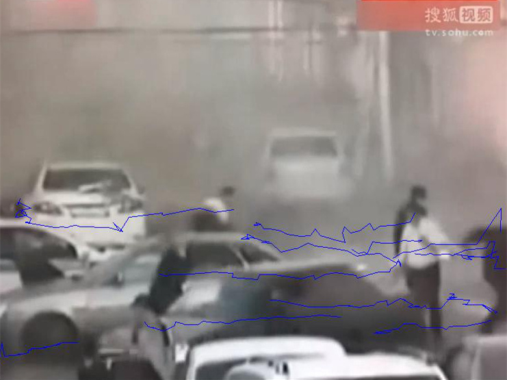
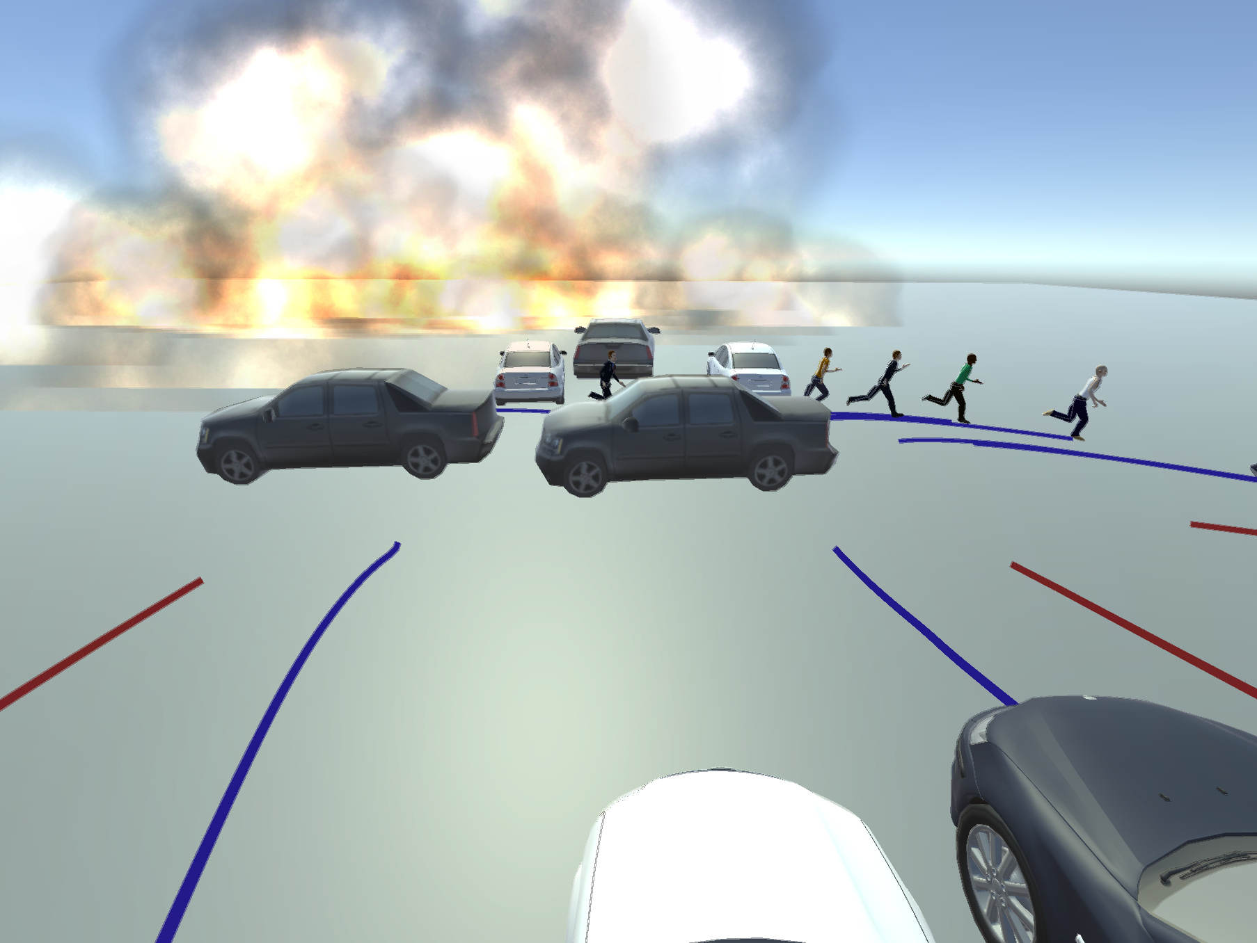
(a)	(b)
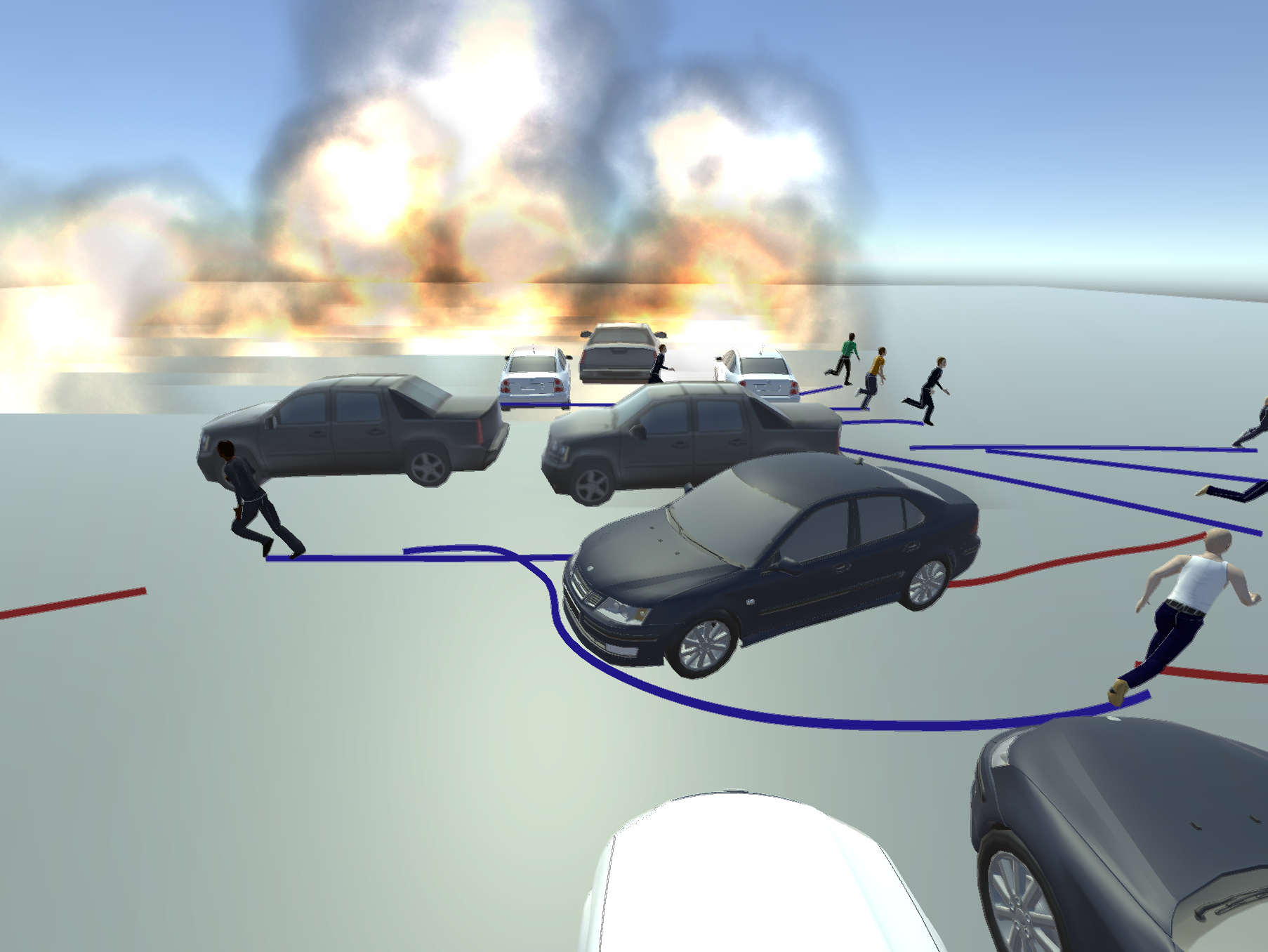
(c)	(d)
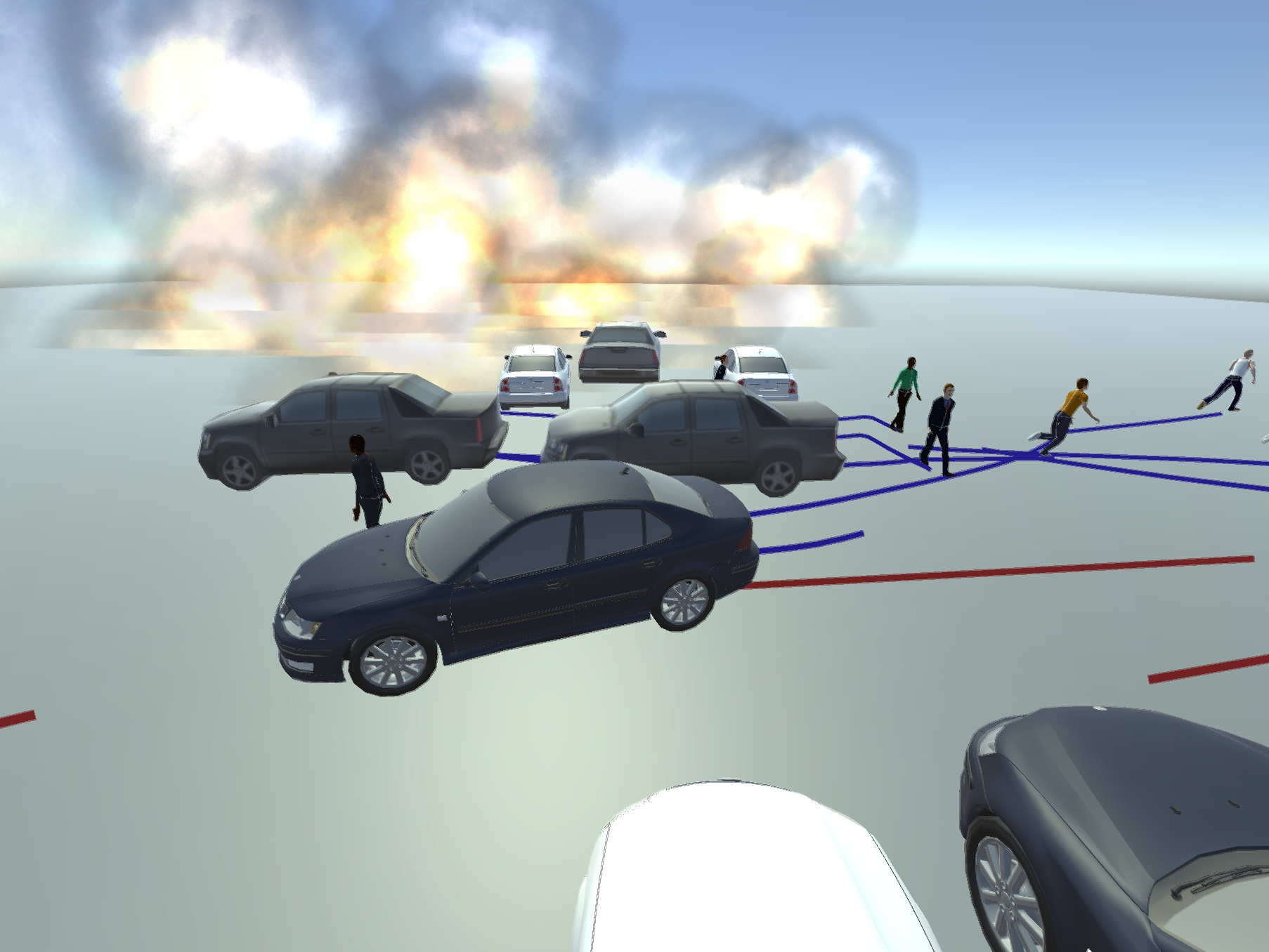
(e)	(f)

Figure 9: Crowd simulation results by different models in the scenario including both crowd and vehicles at the $88th$ frame: (a) Real-world scenario, (b) Neto model, (c) Neto-PS model, (d) Durupinar model, (e) Durupinar-PS model, and (f) our model.

Our proposed algorithm is used to simulate crowd movement in various scenarios and we demonstrate the benefits of it in these different scenarios. We evaluate our model on the public UMN dataset [65] (Figures 4). The dataset comprises the videos of 11 different scenarios of an escape event in 3 different indoor and outdoor scenes. Each video begins with initial normal behavior and ends with sequences of abnormal behavior. In addition, some real-world scenes (Figures 7, 9, and 10) are chosen from real emergency incidents to evaluate our model. The simulation results show that our proposed method can generate realistic group behaviors. It can also reliably predict the changes of physical strength consumption and panic levels of a crowd in an emergency. We also use our proposed model in different virtual scenarios, such as a subway station and a crosswalk. These scenes have dense crowds and the probability of hazard occurrence in these scenarios is high. We simulate the crowd movement in these scenarios after one hazard.

We have implemented the proposed model using Visual C++ to simulate crowd movements in emergencies. The Unity3D game engine has been used to visualize our crowd simulation results. The computing platform corresponds a PC with a quadcore 2.50 GHz CPU,16 GB memory, and an Nvidia GeForce GTX 1080 Ti graphics card. The parameter values in different scenarios used in the simulation are listed in Table III. The mass of each individual is set to 60kg on average and the radius to 0.3m (in Table III) [66]. Each factor of the vector $<O,C,E,A,N>$ is randomly distributed with a Gaussian distribution $N(0,0.25)$ [6]. In most scenes, the dose values $d_{i}$ are randomly distributed with a Gaussian distribution $N(0.1,0.01)$ [6]. In the Neto model, $\epsilon=0.5$, $\delta=0.5$, $\eta=0.5$, and $\beta=1$ [40]. The parameter values are obtained by comparing the simulations with real-world videos. A combination of genetic and greedy strategies are used to sample plausible parameters for our model, maximizing the match of the simulation algorithm to real data [63].

TABLE III: List of parameter values used in our simulations

Scenarios	Model	Num	$R_{a}$	T1					T2			PR	$d_{i}$	$v^{\text{NOR}}$	$v^{\text{MAX}}$	size of scene	$\epsilon$	$\delta$	$\eta$	$\beta$
				$\alpha$	$\beta$	$\gamma$	C	N	$\delta$	$\xi$	E
Grass	Ours	16	0.3	0.1	0.1	0.15	N(0,0.25)	N(0,0.25)	0.35	0.1	N(0,0.25)	10	N(0.1,0.01)	2	0.8	230*111	-	-	-	-
Grass	Durupinar	16	0.3	-	-	-	-	-	-	-	-	10	N(0.1,0.01)	2	0.8	230*111	-	-	-	-
Grass	Neto	16	0.3	-	-	-	-	-	-	-	-	10	-	2	0.8	230*111	0.5	0.5	0.5	1
Room	Ours	19	0.3	0.1	0.1	0.15	N(0,0.25)	N(0,0.25)	0.35	0.1	N(0,0.25)	10	N(0.1,0.01)	2	0.8	25.6*53.5	-	-	-	-
Room	Durupinar	19	0.3	-	-	-	-	-	-	-	-	10	N(0.1,0.01)	2	0.8	25.6*53.5	-	-	-	-
Room	Neto	19	0.3	-	-	-	-	-	-	-	-	10	-	2	0.8	25.6*53.5	0.5	0.5	0.5	1
phone explosion	Ours	152	0.3	0.1	0.1	0.15	N(0,0.25)	N(0,0.25)	0.35	0.1	N(0,0.25)	8	N(0.1,0.01)	2	0.8	600*600	-	-	-	-
British Parliament building	Ours	37	0.3	0.1	0.1	0.15	N(0,0.25)	N(0,0.25)	0.35	0.1	N(0,0.25)	15	N(0.4,0.01)	2/2.5	0.8/1.2	600*600	-	-	-	-
Virtual scenario	Ours	300	0.3	0.1	0.1	0.15	N(0,0.25)	N(0,0.25)	0.35	0.1	N(0,0.25)	10	N(0.1,0.01)	[2,4.5]	[0.8,1.2]	600*600	-	-	-	-
Virtual scenario	Cube-Neto	300	0.3	-	-	-	-	-	-	-	-	10	-	[2,4.5]	[0.8,1.2]	600*600	0.5	0.5	0.5	1
Virtual scenario	Durupinar	300	0.3	-	-	-	-	-	-	-	-	10	N(0.1,0.01)	[2,4.5]	[0.8,1.2]	600*600	-	-	-	-
Virtual Scenario	Neto	300	0.3	-	-	-	-	-	-	-	-	10	-	[2,4.5]	[0.8,1.2]	600*600	0.5	0.5	0.5	1

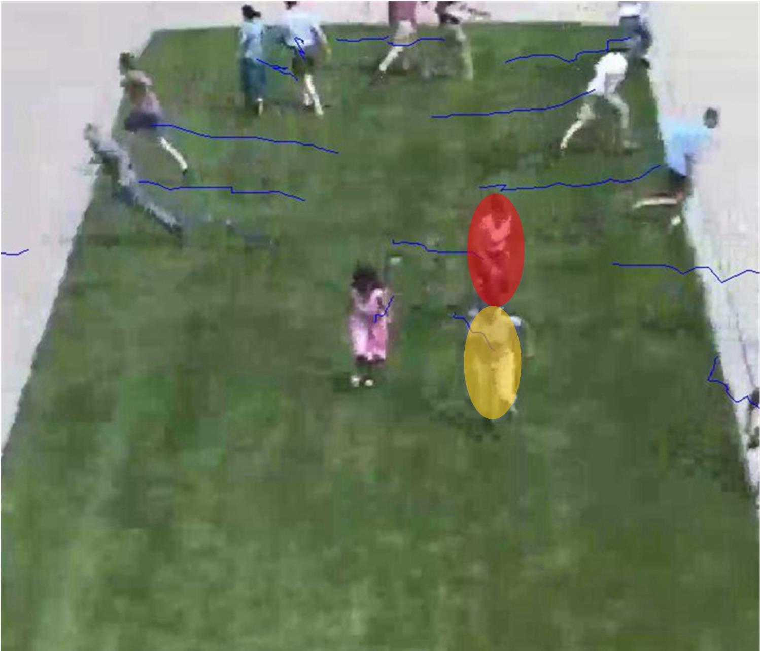
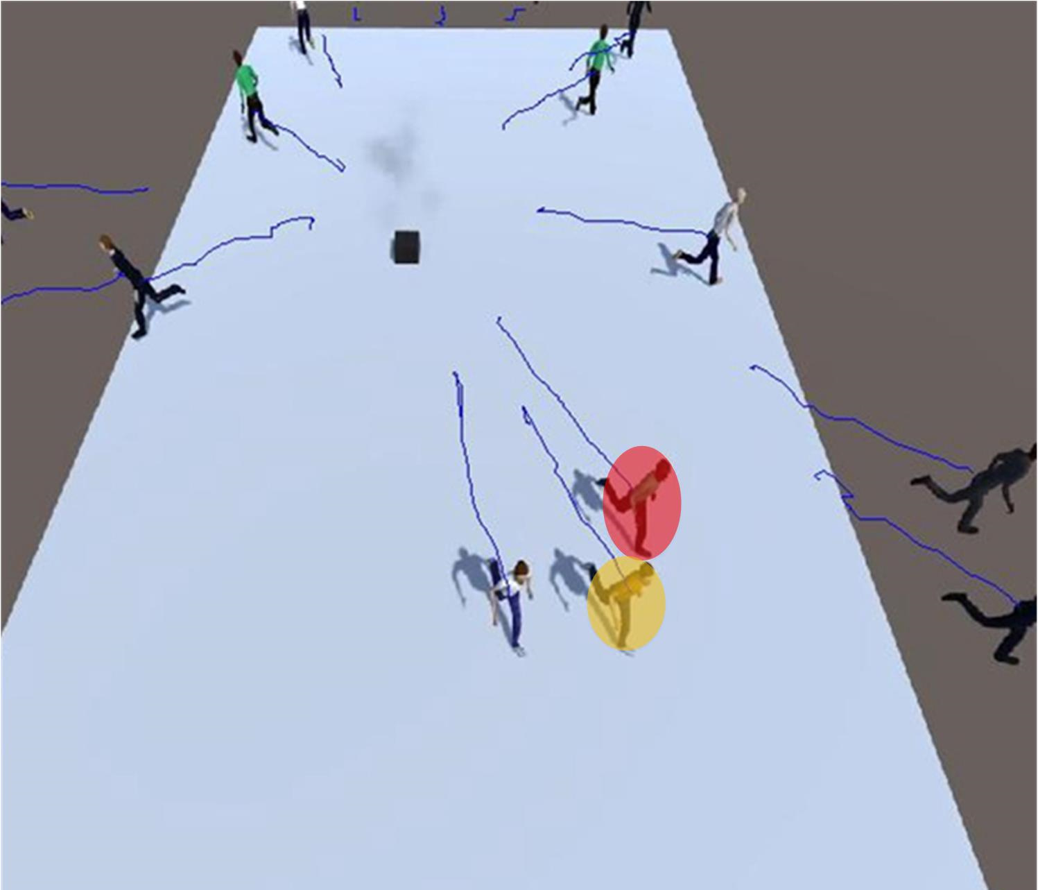
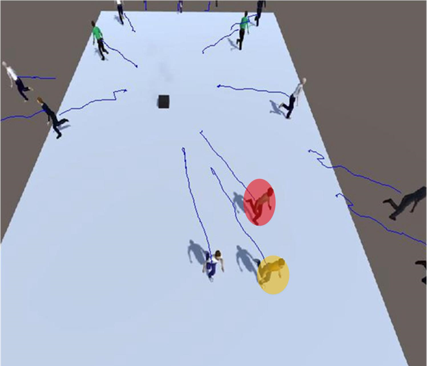
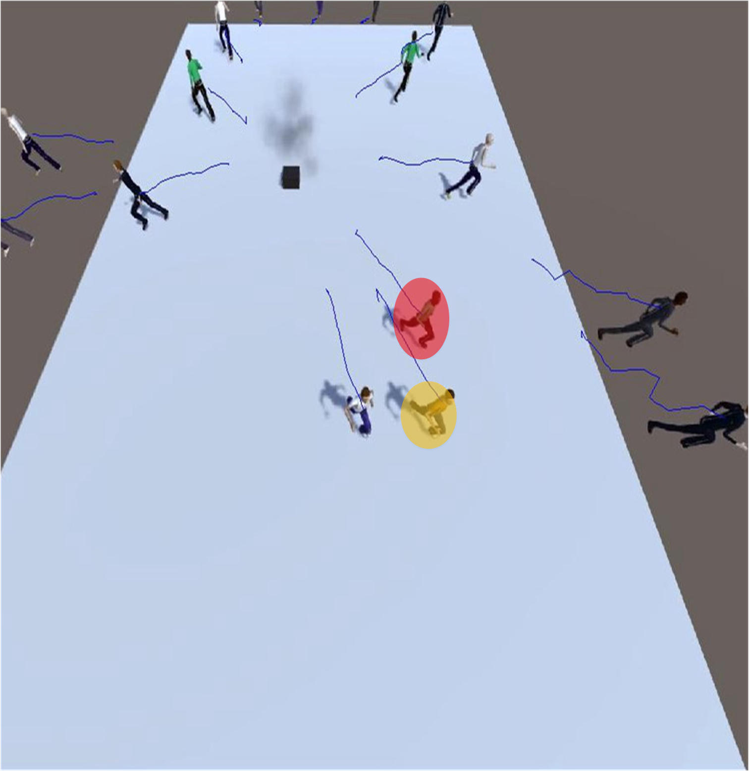
(a)	(b)	(c)	(d)
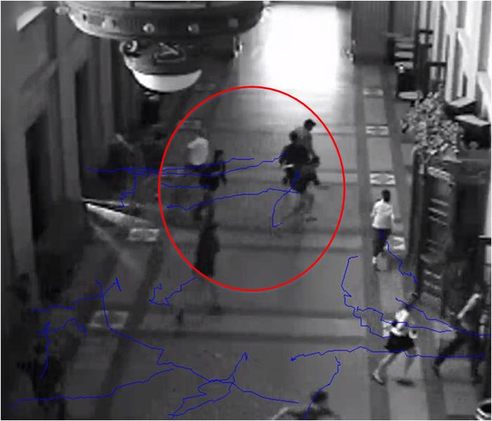
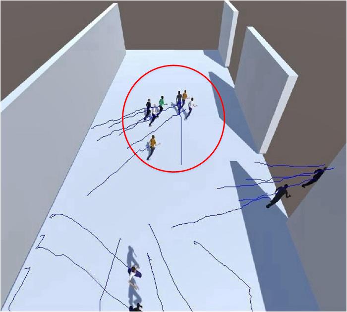
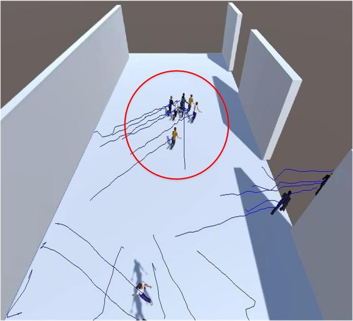
(e)	(f)	(g)	(h)

Figure 4: Comparisons between real scenes and simulation results by different models: (a) and (e) are real-world videos, (b) and (f) are simulated by our model, (c) and (g) are simulated by the Durupinar model, (d) and (h) are simulated by the Neto model. Each row represents one scene. (a) The red ellipse is Individual No. 1 and the yellow one is Individual No. 2. Individual No. 1 gets closer to Individual No. 2. (b) As the speed is influenced by physical strength consumption, simulating the situation where Individual No. 1 gets closer to Individual No. 2 is easier using our model. In (g) and (h), the simulation trajectories of different individuals in the red circle by the Durupinar and Neto model are similar and individuals easily get together, which is different from the real-world video.

4.1 Comparisons

To validate our approach, we compare the simulation results obtained by different methods with real-world crowd evacuation videos. The trend in the simulation results obtained by our model is that they are more similar to real-world videos than results from other approaches.

4.1.1 Comparisons with scenarios from public UMN dataset

Comparisons between real scenes (chosen from the public UMN dataset [65]) and the corresponding simulation results are presented in Figure 4. We take two different real-world scenarios as examples, and detailed results can be seen in the supplementary video. Our model is compared with two other representative emotion models: the Durupinar model [6] and the Neto model [40]. We annotate the trajectories of all the individuals in the real-world video using the video annotation tool in [67] and assign initial movement states to these models. Therefore, we can predict the trajectories of these individuals and compare them with the actual ones.

In the Grass scenario, Individual No. 1 moves faster than Individual No. 2, and Individual No. 1 moves closer to Individual No. 2 (Figure 4a). The simulation result obtained by our model in the Grass scenario is more realistic than those obtained by the Durupinar and Neto models because the speed is influenced by physical strength consumption in our model. If an individual has consumed more physical strength than other individuals, his moving speed decreases and other individuals move faster than he does. Thus, simulating the situation is easier when one individual gets closer to another individual.

In the Room scenario, some individuals are marked with red circles in the simulation results obtained by the Durupinar and Neto models (Figures 4g and 4h). The moving directions and moving speeds of these individuals are almost the same. The simulation result by our model conforms to the real-world video. This is because the emotion mechanism of our model changes the moving directions of individuals and drives them to move away from the hazard. Meanwhile, the physical strength consumption influences the individual’s speed.

We use the entropy metric [68] to evaluate the trajectories of different simulation algorithms on different scenarios. Entropy metric is used to measure the similarity between real-world data and simulation results. A lower value of the entropy metric means a smaller error and better similarity with the real-world data. Its calculation method is described as follows. The real-world crowd state is denoted as $({{x}_{1}}\ldots{{x}_{t}})$, which includes the positions of all the agents at different timesteps. $({{y}_{1}}\ldots{{y}_{t}})$ is the corresponding calculation result of our model. $M$ is the estimated error variance.

where $t$ is the total number of timesteps and $n$ is the number of agents in the scenario. The Entropy metric is given by:

$${e(\mu)=\frac{1}{2}n\log({{(2\pi e)}^{d}}\det(M))}$$ (33)

where $d$ is the dimension of the state of a single agent. In this paper, we mainly discuss the 2D locations of agents. So, $d=2$ in this paper.

For each scenario, a user study is performed. There are 39 participants (51.28$\%$ female, 66.67$\%$ in the age group of 20-30) in this study and participants are asked to compare the movement states in the original video clips with the movement states in the crowd simulation results (Figure 5). These similarity scores are computed from the user studies. A score of 1 indicates most dissimilar and a score of 5 indicates most similar movement. Higher values indicate greater similarity. We also calculate average spatial distance between the simulated results and the ground truth over all the timesteps and individuals. Tables IV and Figure 5 show that the simulated moving trends of our model are closer to those in the real-world videos than the results of other models. A rational approach is to combine physical strength consumption and panic to determine the movement of each individual.

TABLE IV: Entropy metric and spatial distance for different simulation algorithms on scenarios of Grass and Room. A lower value implies higher similarity with respect to the real-world crowd videos.

Scenario	Model	Entropy metric	Spatial distance
Grass	Ours	3.386800	1.042990
	Durupinar	3.429000	1.105531
	Neto	3.409700	1.046776
Room	Ours	5.393900	1.481327
	Durupinar	5.463200	1.484492
	Neto	5.493300	1.527570

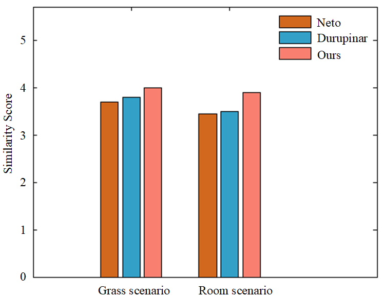
Figure 5: Comparison of similarity scores for movement states (higher values indicate greater similarity). We compare the movement states in the original videos with those in crowd simulation results achieved by different algorithms.

(a)	(b)
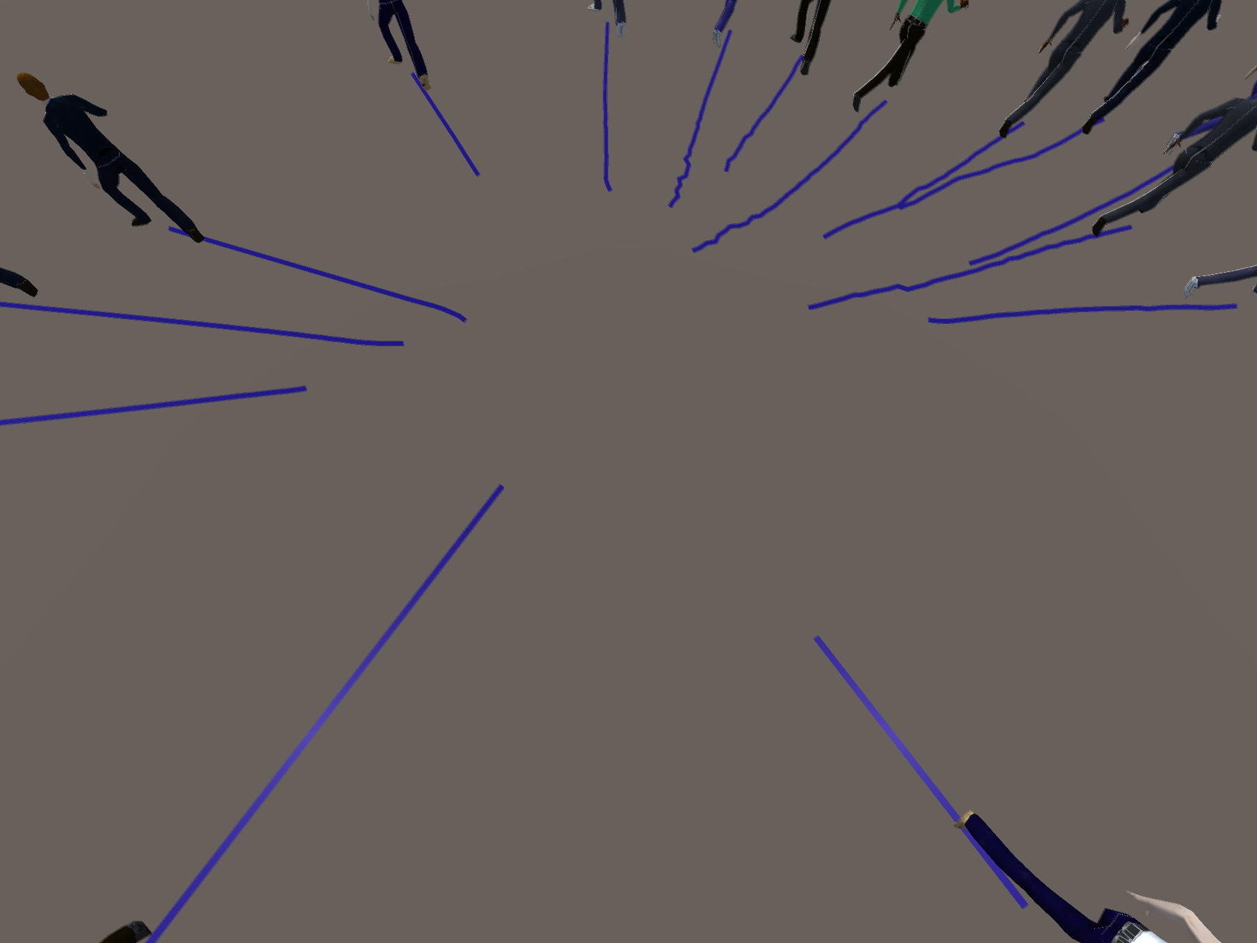
(c)	(d)
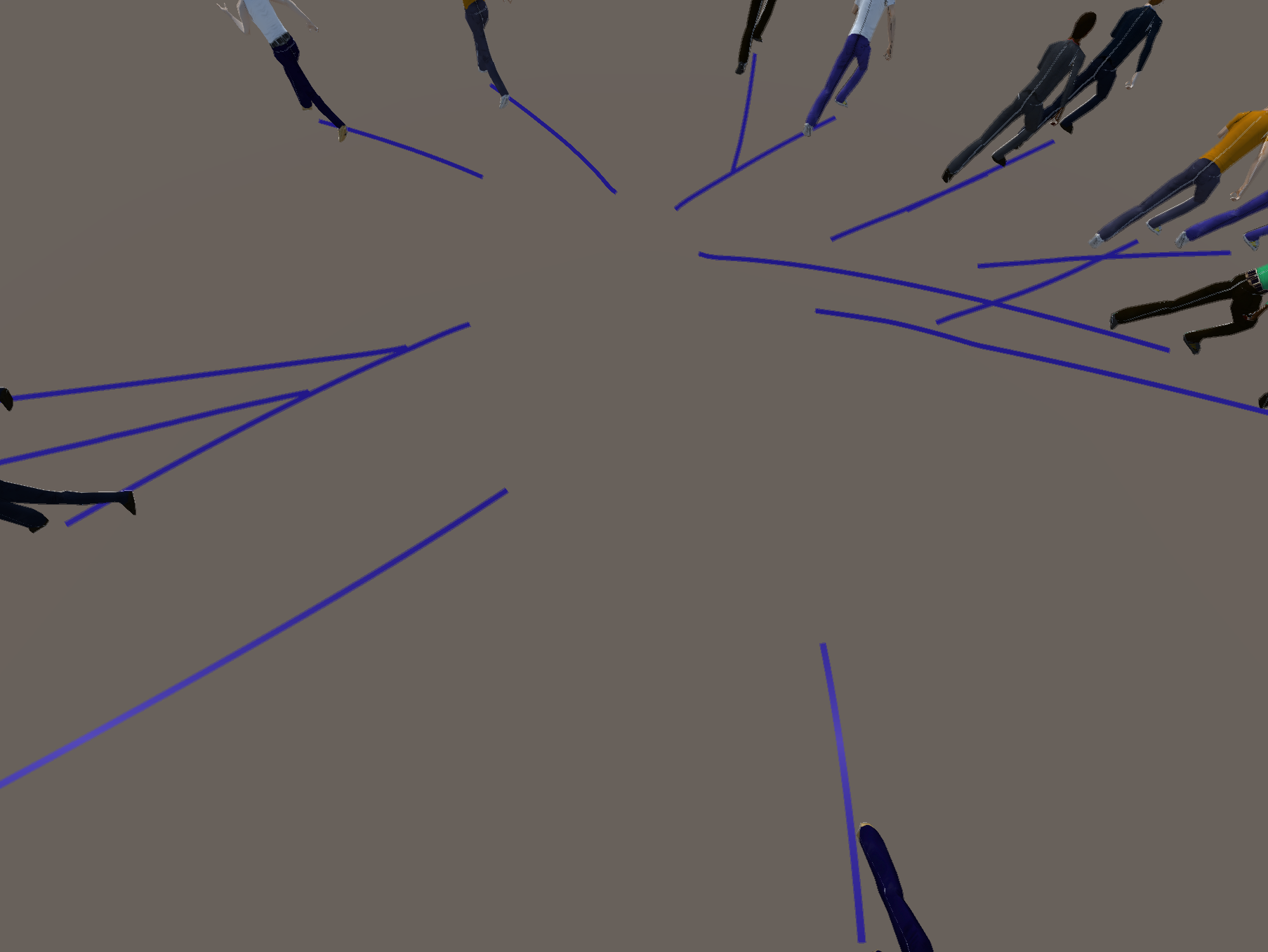
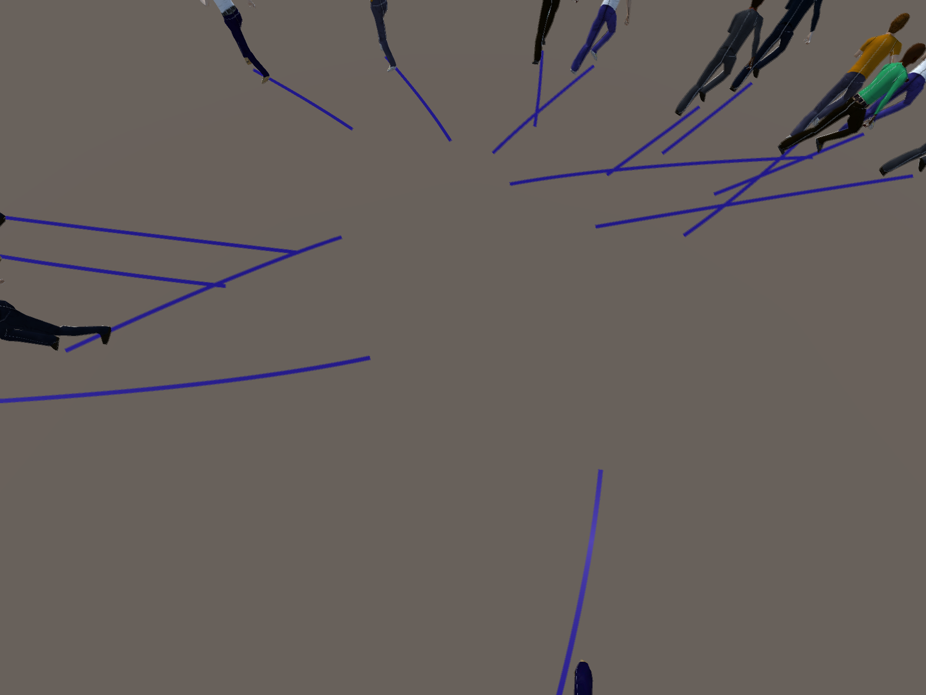
(e)	(f)

Figure 6: Crowd simulation results generated by different models in the Square scenario at the $98th$ frame: (a) Real-world scenario, (b) Neto model, (c) Neto-PS model, (d) Durupinar model, (e) Durupinar-PS model, and (f) our model.

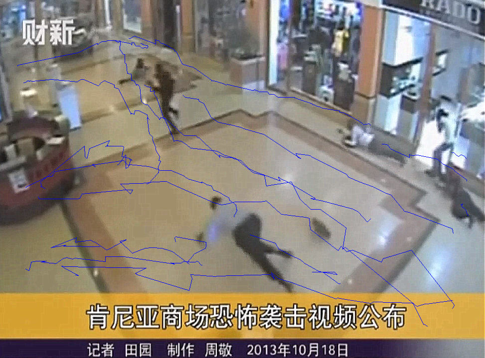
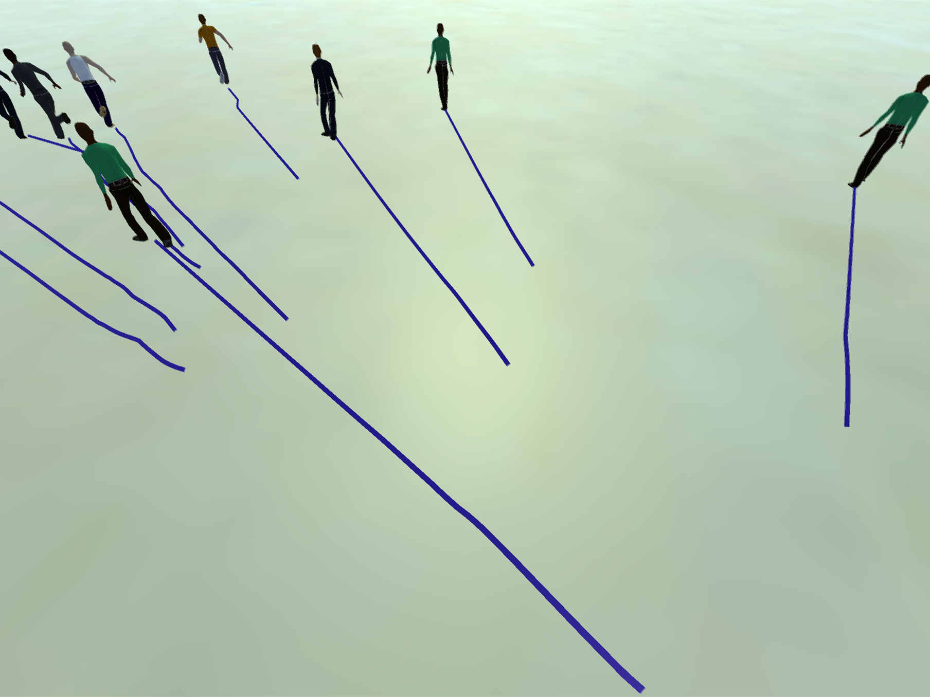
(a)	(b)
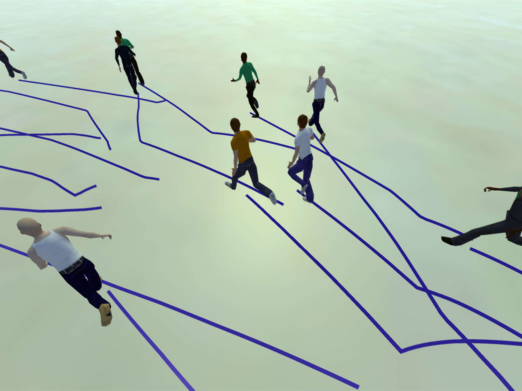
(c)	(d)
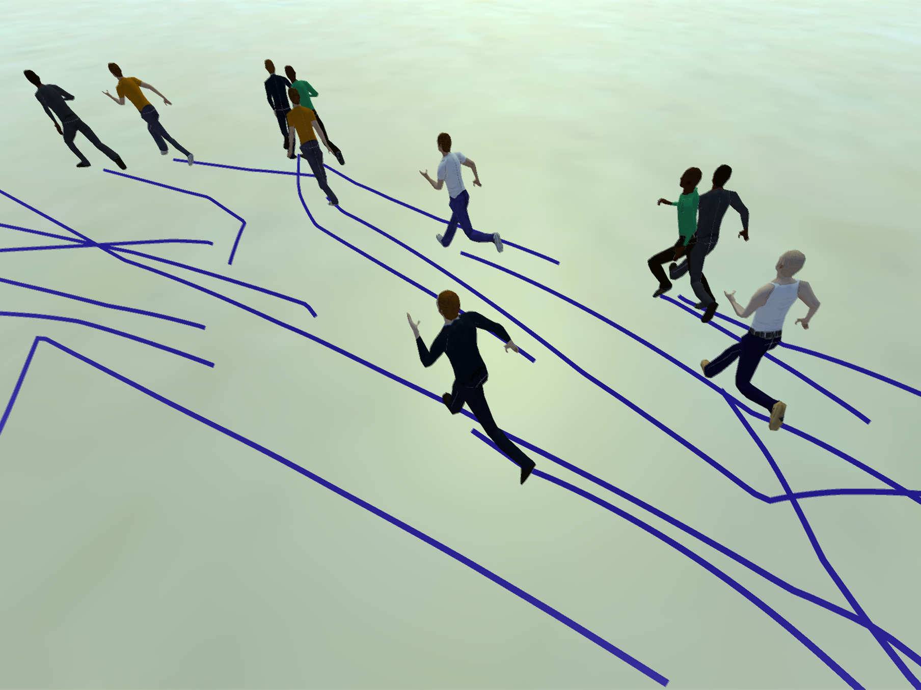
(e)	(f)

Figure 7: Crowd simulation results by different models in the scenario of terrorist attacks on Kenya’s shopping mall at the $214th$ frame: (a) Real-world scenario, (b) Neto model, (c) Neto-PS model, (d) Durupinar model, (e) Durupinar-PS model, and (f) our model.

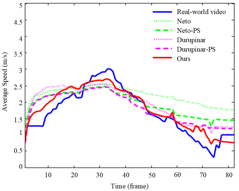
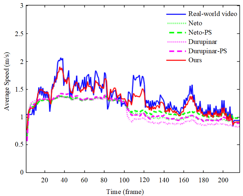
Figure 8: The average speeds of all the individuals at different timesteps for these different models in (a) the Square scenario and (b) the scenario of terrorist attacks on Kenya’s shopping mall. The average speeds of our model at different timesteps are closer to the real scene than those of other models. The average speeds of the Neto-PS and Durupinar-PS models at different timesteps are closer to the real-world scenarios, than those of the original Neto and Durupinar models.

4.1.2 Comparisons with real-world emergency scenarios

In this subsection, we compare the simulation results obtained by different methods with real-world videos, particularly real emergency incidents.

The Durupinar and Neto models don’t consider physical strength consumption. The mechanism of physical strength consumption in this paper is integrated into these two models, which are denoted as Durupinar-PS and Neto-PS. In the real-world Square scenario, we compare our simulation results with the Durupinar, Durupinar-PS, Neto, and Neto-PS models (Figure 6). We also compare our results in a real-world emergency scenario, which is related to terrorist attacks on Kenya’s shopping mall (Figure 7). More details can be seen in the supplementary video. Figure 8 shows the average speeds of all the individuals at different timesteps for these different models. We find that the simulation results of the Durupinar-PS and Neto-PS are closer to the movements and behaviors in the real videos, than those of the original Durupinar and Neto models. These comparisons validate that our proposed mechanism of physical strength consumption (physical strength consumption calculation and the effect of physical strength consumption on emotion) can enhance the performance of existing crowd simulation models that are only based on emotion. Our model describes emotional changes in a comprehensive manner. Based on the James-Lange theory, we describe three stages individual emotions undergo (Section 3.3.2) and combine emotional contagion with the effect of physical strength consumption on panic. The comparisons with Durupinar-PS and Neto-PS models show that our model integrating emotion and physical strength consumption is better than other emotion-based crowd simulation models.

One piece of real-world video including both crowd and vehicles is chosen to simulate by our method. In this real scenario, we compare our simulation result with the Durupinar, Durupinar-PS, Neto, and Neto-PS models. In this paper, we mainly focus on emotions of crowds, especially panic emotions in emergencies. In particular, the drivers can express their panic through vehicles. Moreover, in emergencies, the drivers may not follow the traffic rules. In emergency scenarios, some behaviors of vehicles, such as sudden acceleration, intuitively demonstrate the drivers’ panic. These behaviors can also cause the surrounding pedestrians to be panicked and thus act indirectly as emotional contagions. In common cases, when pedestrians are walking in front of vehicles, vehicles will slow down, change direction, or stop to avoid pedestrians. Vehicles and surrounding pedestrians influence each other in such traffic. Based on above analysis, in our model we treat vehicles as one kind of special large-sized agents with full physical strength and high moving speed. The radius of the vehicles is set to 3. The comparisons show that our simulation result conforms to the real-world video, and can enhance the performance of existing crowd simulations under the complex scenarios including both crowd and vehicles. More details can be seen in the supplementary video.

Table V shows the values of entropy metric and spatial distance for the above three scenarios. Comparing with the Durupinar, Durupinar-PS, Neto, Neto-PS models, our model can generated more similar simulation results with real-world scenarios.

TABLE V: Entropy metric and spatial distance for different simulation algorithms on scenarios of Square, Crowd and vehicles, and Terrorist attacks on shopping mall. A lower value implies higher similarity with respect to the real-world data.

Scenario	Model	Entropy metric	Spatial distance
Square	Ours	1.278777	0.210871
	Durupinar	3.292511	0.316492
	Durupinar-PS	1.883470	0.238043
	Neto	3.415817	0.327066
	Neto-PS	1.568437	0.220118
Crowd and vehicles	Ours	3.740438	0.816685
	Durupinar	5.851273	2.402975
	Durupinar-PS	5.785572	2.067541
	Neto	5.984731	2.346846
	Neto-PS	5.768604	2.070267
Terrorist attacks on shopping mall	Ours	1.060493	0.225969
	Durupinar	5.782041	0.761416
	Durupinar-PS	3.809553	0.405739
	Neto	5.783371	0.755286
	Neto-PS	3.230872	0.382926

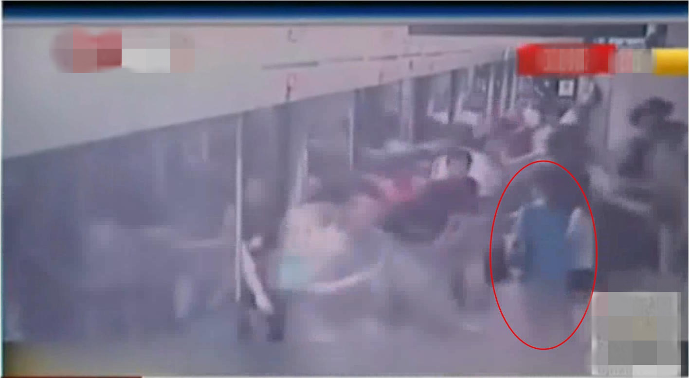
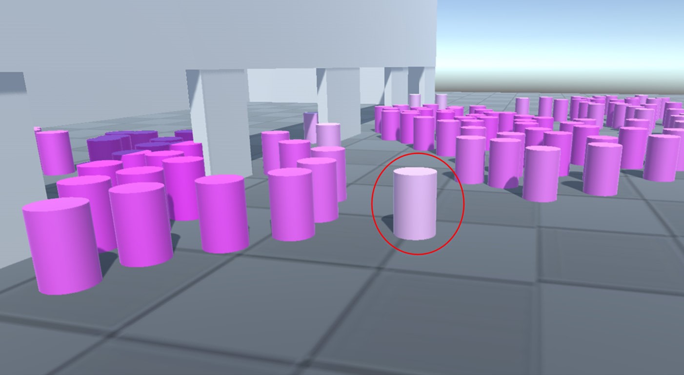
(a)	(b)
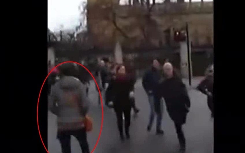
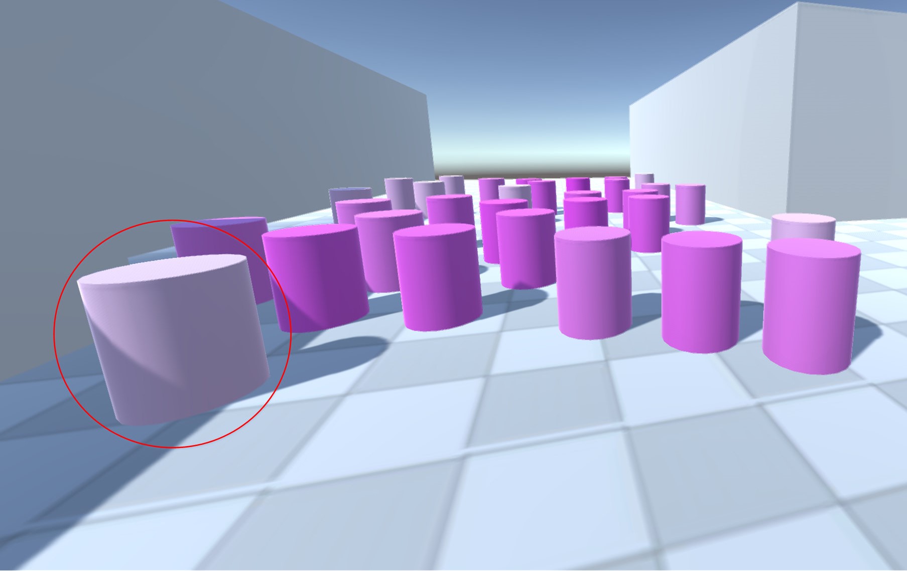
(c)	(d)

Figure 10: Comparisons between real-world videos and simulation results by our approach. (a) The mobile phone explosion incident on the subway in the Shanghai Metro Line 8; (c) the shooting incident at the British Parliament building on March 22, 2017; (b,d) our corresponding simulation results. At first, the individuals in the red circle aren’t panicked. Because of emotional contagion, they are then influenced by the panicked crowd around them, become panicked, and run away from the hazards.

We also take two real emergency incidents as examples to verify our proposed crowd simulation method. Our crowd simulation results of the scene after the mobile phone explosion on the subway in the Shanghai Metro Line 8 are presented in Figures 10a and 10b. Crowd simulation by our model of the shooting at the British Parliament building on March 22, 2017 is presented in Figures 10c and 10d. We show the spread of panic in both scenarios. The color of the cylinders represents the emotional intensity of the individuals. These two real-world videos have poor quality images. Even using manual methods, it is still difficult to track the positions of people in each frame accurately. Due to these objective limitations, we cannot measure the similarity between the simulated trajectories and the ground truth for these scenes in a direct way. Therefore, we use the dominant path and entropy metric to quantitively evaluate our simulation results. The dominant path is defined based on collectiveness of crowd movements and it can be treated as the movement trend of the crowd [69, 70]. We also calculate the spatial distance between the simulated trajectories and the ground truth for the scenarios. From Table VI and Figure 11, we can see that both the overall moving trend and the process of emotional contagion are similar to what is found in the recorded real-world crowd video clips.

TABLE VI: Entropy metric and spatial distance for different simulation algorithms on scenarios of Phone explosion and Shooting at British Parliament.

Scenario	Model	Entropy metric	Spatial distance
Phone explosion	Ours	1.565650	1.137298
	Durupinar	4.826474	1.523882
	Neto	2.857793	1.495380
Shooting at British Parliament	Ours	0.842232	0.749183
	Durupinar	2.246331	0.784255
	Neto	1.626734	0.771396

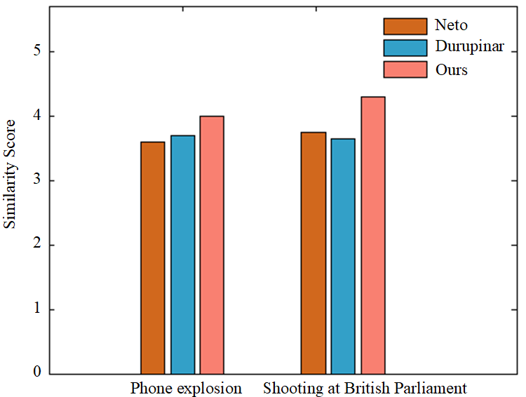
Figure 11: Comparison of similarity scores for movement states and the process of emotional contagion (higher values indicate greater similarity). A user study is performed and participants are asked to compare the movement states and processes of emotional contagion in the original videos with those in crowd simulation results achieved by different algorithms.

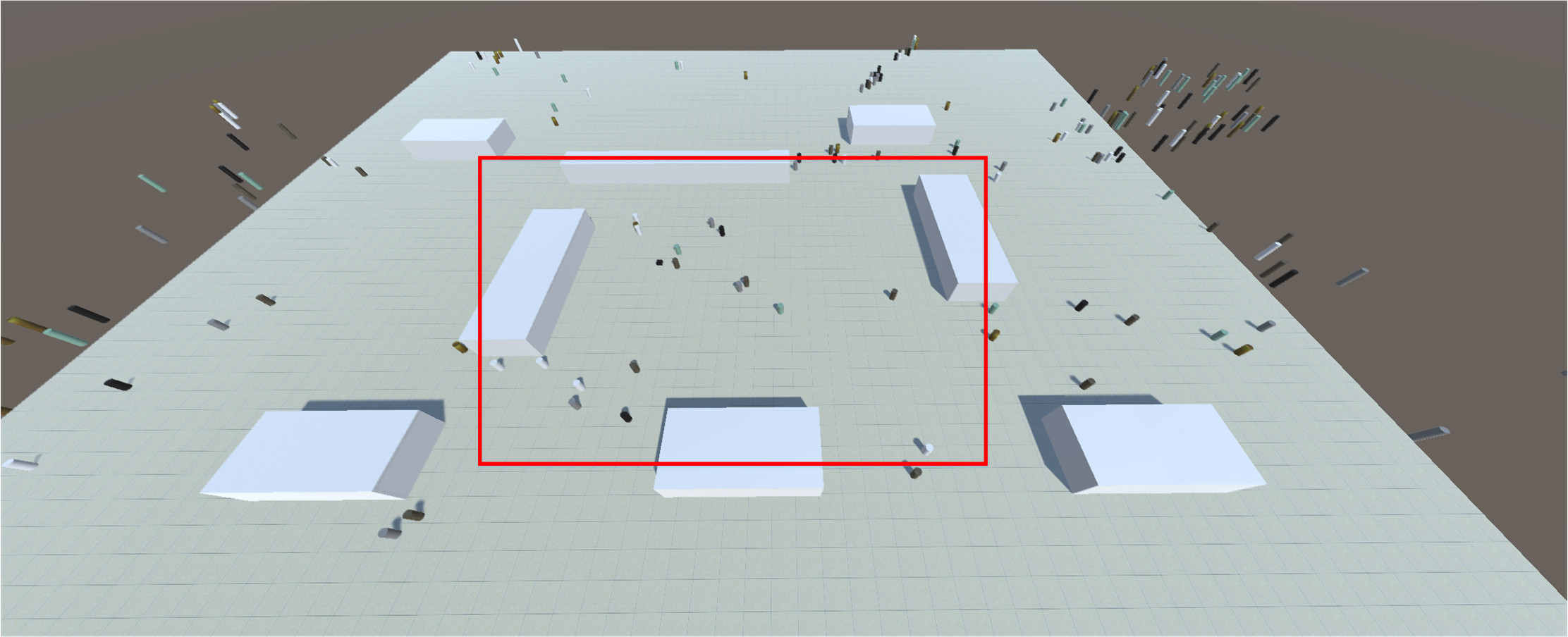
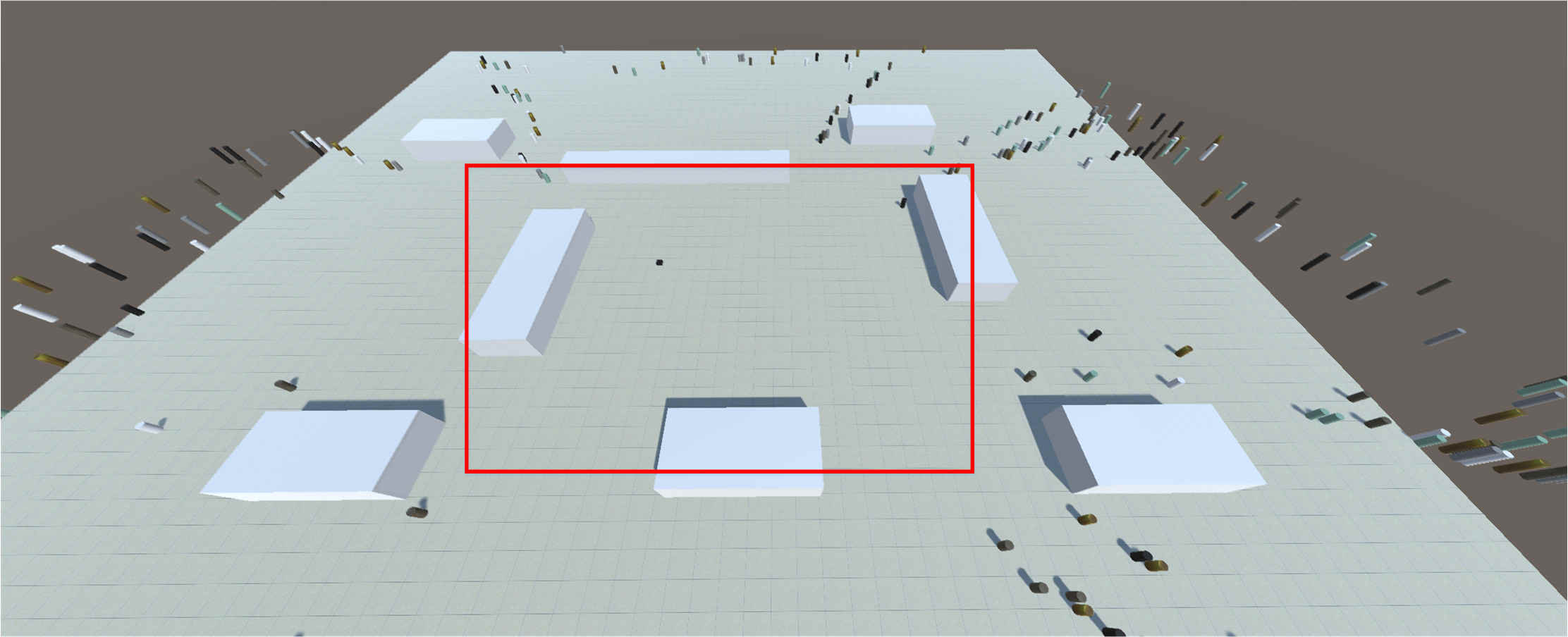
(a)	(b)
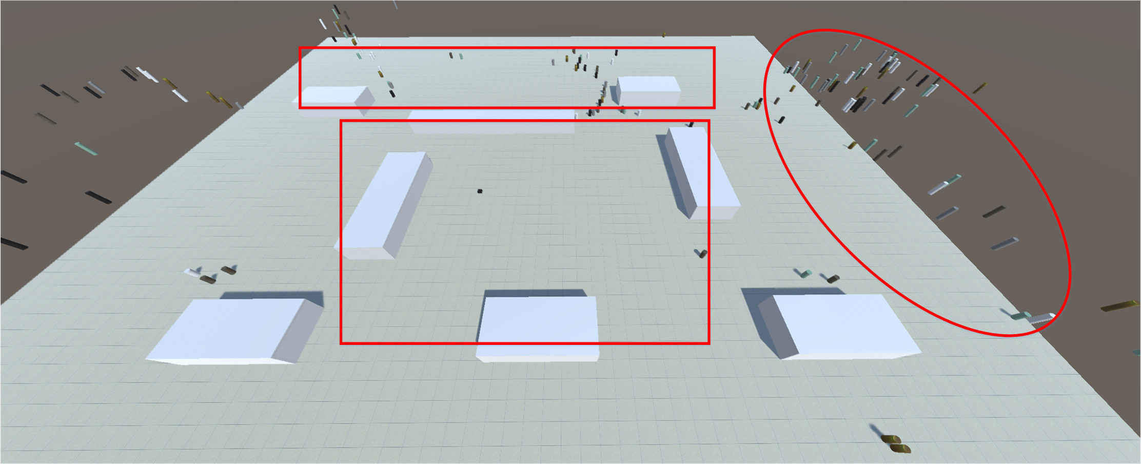
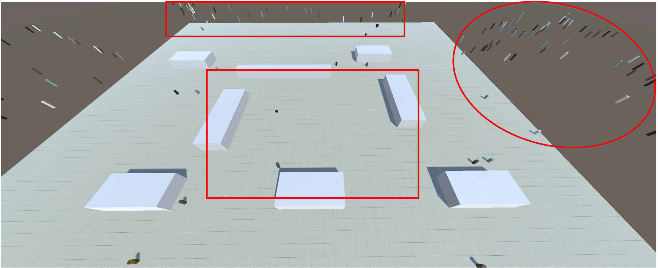
(c)	(d)

Figure 12: Crowd simulation results by different models in the virtual scenario at the $1000th$ frame: (a) Durupinar model, (b) Neto model, (c) Ours-Neto model, and (d) our model.

4.1.3 Comparisons in virtual scenarios

In the virtual scenario, we compare our simulation results with those of the Durupinar [6], Neto [40], and Ours-Neto models. The parameter values we used are described in Table III. In Figure 12a (the simulation result by the Durupinar model), the speeds of individuals are variable and their locations are scattered. Because of different thresholds and personality mechanisms, the Durupinar model can simulate heterogeneous crowd behaviors. However, there are too many individuals who are not affected by the panicked crowd and this result is unreasonable. In Figure 12b, individuals move much slower than the individuals in the simulation results by other models. The reason is that the emotion calculated by the Neto model is much smaller. Moreover, the individual movement is too regular, which is unsuitable for emergency situations. In Figure 12c (simulation result by our model with the same emotional contagion method as the Neto model) and Figure 12d (our simulation result), most of the individuals are affected by the hazard and run away from it. Because of physical strength consumption and personality factors, the speeds of individuals in our simulation result are more variable than those shown in the Ours-Neto model. Therefore, the simulation result by our model is more suitable for emergency situations than other models.

4.2 Application of our model in various virtual scenarios

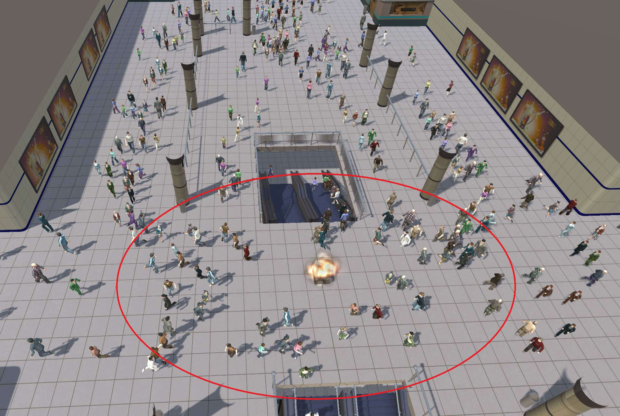
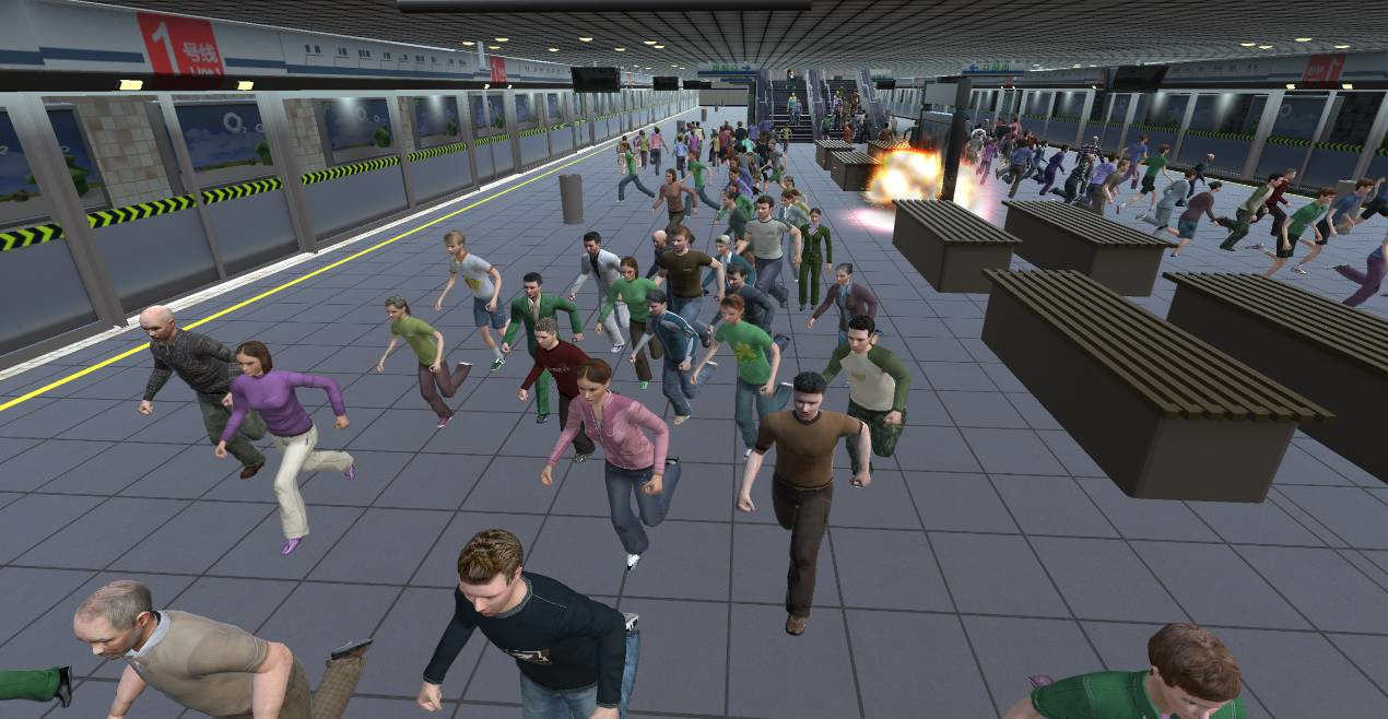
Figure 13: Crowd simulation results at a subway station: (a) the higher level of the subway station, (b) the lower level of the subway station. After the hazard occurs, the emotional contagion in our model begins to work. Although the direct impact of the hazard is limited, the hazardous area grows through emotional contagion among individuals and the number of individuals who run away from the hazard increases.

Our model can be applied in different virtual scenarios. Subway stations and crosswalks are crowded and the probability of hazard occurrence in these scenarios is very high. We simulate a hazard occurring in these scenarios and three examples are shown. Figure 13(a) shows crowd simulation at the higher level of the subway station. Figure 13(b) shows crowd simulation at the lower level of the subway station. Figure 14 shows crowd simulation at a crosswalk. We show each step of the process: hazard occurring, individuals running away from the hazard, emotional contagion spreading, and moving speed attenuating. More details can be seen in the supplementary video. Our simulation results provide information about decision-making to deal with emergency situations.

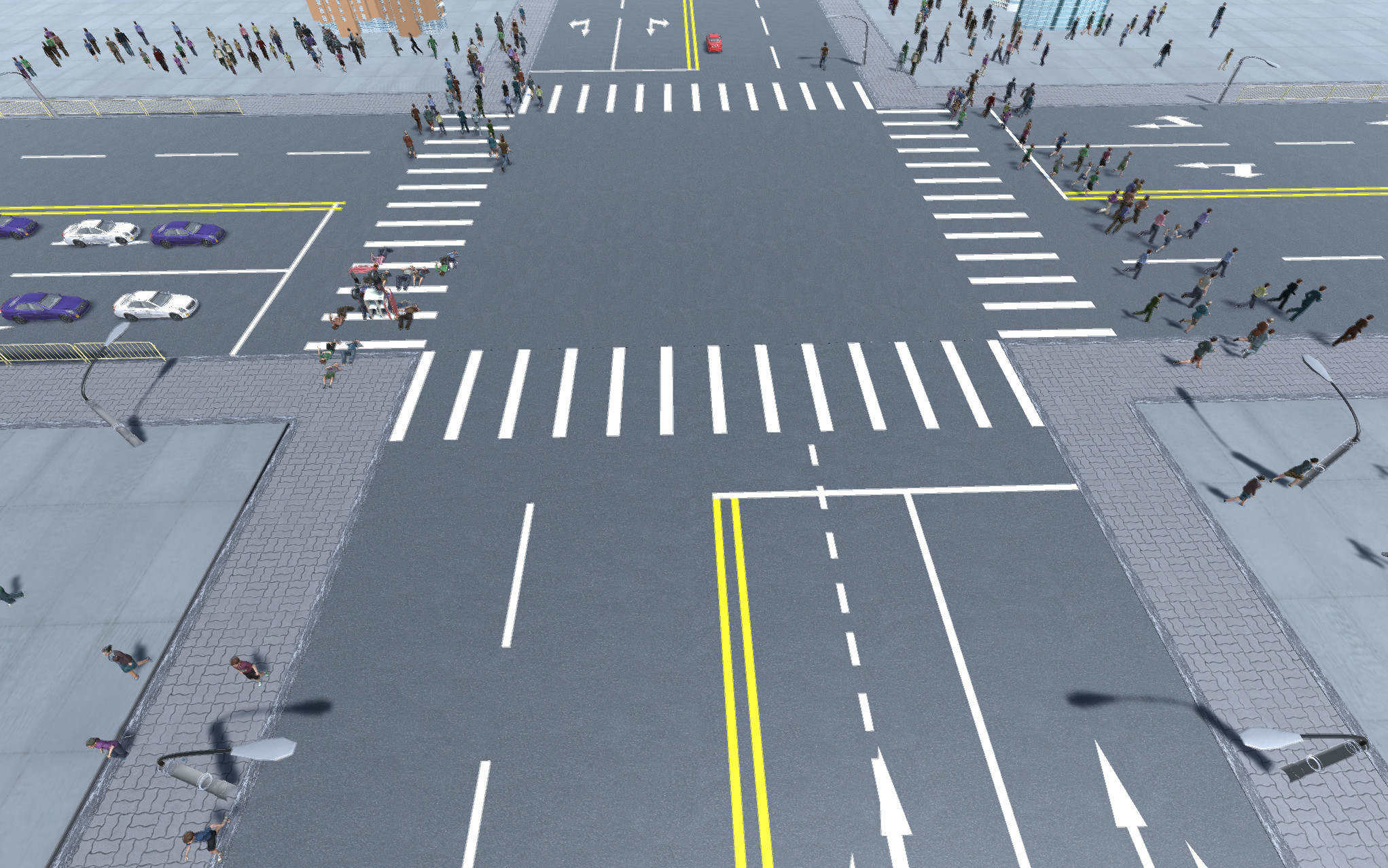
Figure 14: Crowd simulation result at a crosswalk. At the lower left corner, a car explodes. Then individuals run away from the hazard.

The heat maps of panic in the virtual scene are presented in Figure 15. Although the direct impact of the hazard is limited, the panic area grows through the emotional contagion mechanism in our model. When individuals are far from the hazard, panic attenuates. As accidents may happen randomly in public places, we can take preventive action in advance and reduce loss by accurately predicting the panic area.

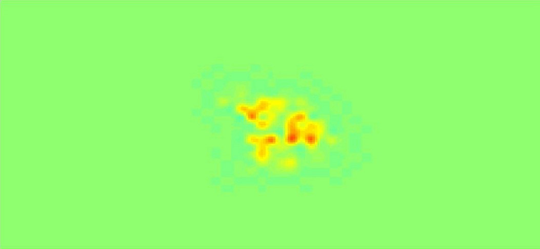
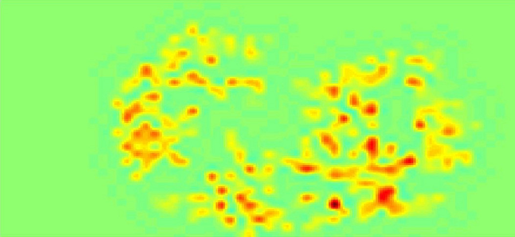
(a)	(b)
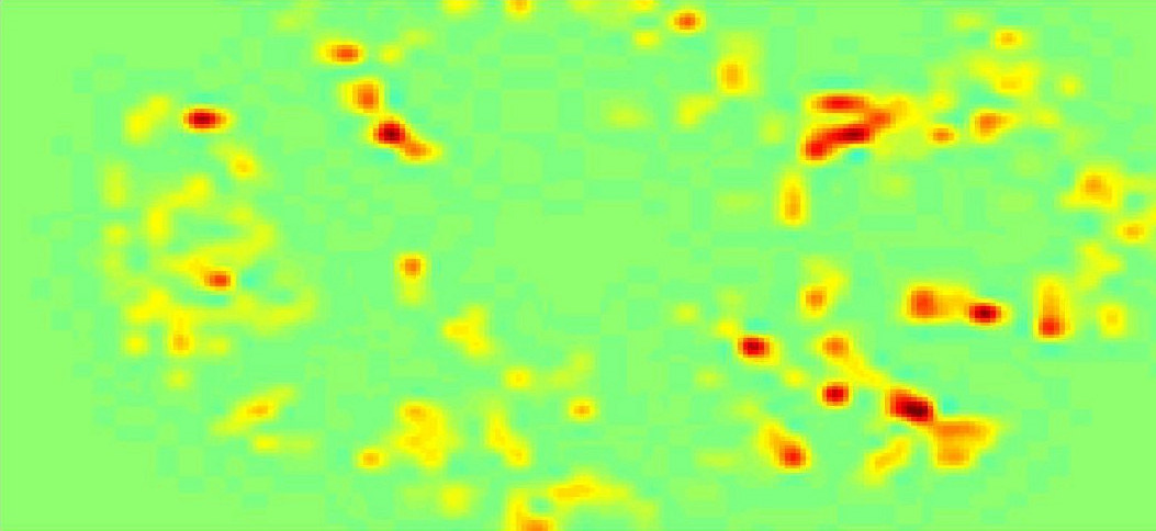
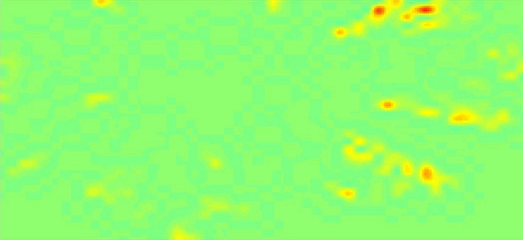
(c)	(d)

Figure 15: Panic heat maps of the virtual scene: (a) heat map at the $13^{th}$ frame, (b) heat map at the $29^{th}$ frame, (c) heat map at the $57^{th}$ frame, (d) heat map at the $120^{th}$ frame. The red area is more panicked than the green area in the heat map. The deeper the color, the more panicked the area.

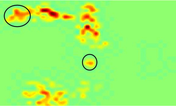
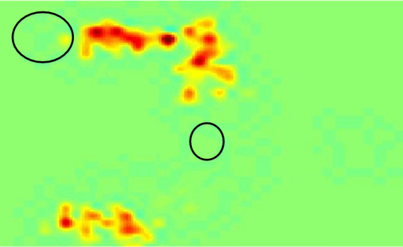
(a)	(b)

Figure 16: The heat maps of panic at the $185^{th}$ frame of the crosswalk scenario: (a) heat map of the crowd simulation generated by our model and (b) heat map of the crowd simulation generated using the Durupinar model. The red area is more panicked than the green area in the heat map. The deeper the color, the more panicked the area. We highlight the same area of the two simulation results. The individuals in our model simulation result are more panicked than the individuals in the Durupinar model simulation results.

The panic heat maps generated from crowd simulations in the crosswalk scenario by our model and those generated using the Durupinar model are presented in Figure 16. The individuals in the simulation results by our model are more panicked than those in the Durupinar model simulation results. The intensity of the panic calculated by the Durupinar model is lower than that calculated by our model. The reason is that our model considers not only emotional contagion among individuals, but also the impact of physical strength consumption on panic levels. Our model represents a comprehensive description of individual panic levels and is more conducive to the spread of panic than the Durupinar model. Therefore, the simulation results by our model are more reasonable for emergency situations.

5 Conclusion and Limitations

In contrast to traditional emotion-based crowd simulation models, we integrate physical strength consumption into our model. We not only present a panic level calculation, but also delineate the effect of physical strength consumption on panic. Finally, both physical strength consumption and panic determine the movement of each individual. Our proposed model is verified by simulations, and it is compared with real-world videos and previous approaches. Results have shown that our proposed model can reliably generate realistic group behaviors. It can also predict the changes of physical strength consumption and panic of a crowd in an emergency situation.

However, our model has several limitations. Although our model can generate realistic crowd movements, the panic levels and physical strength consumption of the crowd in an emergency scene cannot be obtained directly. Our model can only infer them during the simulation. Thus, the initial state of our model is difficult to determine and it is usually time consuming to do so. In the future, we plan to use the latest wearable equipment to collect these data and provide a new method that can quickly and accurately determine the initial state. Furthermore, at present, our model mainly focuses on emergency scenarios. In future work, we want to extend our model to a variety of general situations. We also plan to develop a coupled framework for crowd and traffic flow to generate realistic mixed traffic simulations and model the influence of these two flows on each other.

Mingliang Xu received the Ph.D. degree in computer science and technology from the State Key Laboratory of CAD&CG, Zhejiang University, Hangzhou, China. He is a Full Professor with the School of Information Engineering, Zhengzhou University, Zhengzhou, China, where he is currently the Director of the Center for Interdisciplinary Information Science Research. He was with the Department of Information Science, National Natural Science Foundation of China, Beijing, China, from 2015 to 2016. His current research interests include computer graphics, multimedia, and artificial intelligence. He has authored over 60 journal and conference papers in the above areas, including the ACM Transactions on Graphics, ACM Transactions on Intelligent Systems and Technology, IEEE TRANSACTIONS ON PATTERN ANALYSIS AND MACHINE INTELLIGENCE, IEEE TRANSACTIONS ON IMAGE PROCESSING, IEEE TRANSACTIONS ON CYBERNETICS, IEEE TRANSACTIONS ON CIRCUITS AND SYSTEMS FOR VIDEO TECHNOLOGY, ACM SIGGRAPH (Asia), ACM MM, and ICCV. Dr. Xu is the Vice General Secretary of ACM SIGAI China.

Chaochao Li received the B.S. degree in computer science and technology and the master’s degree in computer application technology from the School of Information Engineering, Zhengzhou University, Zhengzhou, China, where he is currently pursuing the Ph.D. degree. His current research interests include computer graphics and computer vision.

Pei Lv received the Ph.D. degree from the State Key Laboratory of CAD&CG, Zhejiang University, Hangzhou, China, in 2013. He is currently an Associate Professor with the School of Information Engineering, Zhengzhou University, Zhengzhou, China. His current research interests include video analysis and crowd simulation. He has authored over 20 journal and conference papers in the above areas, including the IEEE TRANSACTIONS ON IMAGE PROCESSING, IEEE TRANSACTIONS ON CIRCUITS AND SYSTEMS FOR VIDEO TECHNOLOGY, and ACM Multimedia.

Wei Chen is a professor at the State Key Lab of CAD&CG, Zhejiang University. His research interests are visualization and visual analysis, and he has published more than 30 IEEE/ACM Transactions and IEEE VIS papers. He actively served as guest or associate editors of IEEE Transactions on Visualization and Computer Graphics, IEEE Transactions on Intelligent Transportation Systems, and Journal of Visualization. For more information, please refer to http://www.cad.zju.edu.cn/home/chenwei/.

Zhigang Deng is a Full Professor of Computer Science at University of Houston (UH). He is also the Director of Graduate Studies at UH’s Computer Science Department and the Founding Director of the UH Computer Graphics and Interactive Media (CGIM) Lab. He earned a Ph.D. in Computer Science at the Integrated Media System Center (NSF ERC) and the Department of Computer Science at the University of Southern California in 2006. He completed a B.S. degree in Mathematics from Xiamen University (China), and an M.S. in Computer Science from Peking University (China).His interests are in the broad areas of computer graphics, computer animation, human computer interaction, virtual human modeling and animation, and visual computing for biomedical/healthcare informatics. He is the recipient of ACM ICMI Ten Year Technical Impact Award, UH Teaching Excellence Award, Google Faculty Research Award, UHCS Faculty Academic Excellence Award, and NSFC Overseas and Hong Kong/Macau Young Scholars Collaborative Research Award. Besides being the CASA 2014 conference general co-chair and the SCA 2015 conference general co-chair, he currently serves as an Associate Editor of several journals including Computer Graphics Forum and Computer Animation and Virtual Worlds Journal.

Bing Zhou received B.S. and M.S. degrees from Xi’an Jiaotong University, Xi’an, China, in 1986 and 1989, respectively, and a Ph.D. from Beihang University, Beijing, China, in 2003, all in computer science. He is currently a Professor with the School of Information Engineering, Zhengzhou University, Zhengzhou, China. His current research interests include video processing and understanding, surveillance, computer vision, and multimedia applications.

Dinesh Manocha is the Paul Chrisman Iribe Chair in Computer Science & Electrical and Computer Engineering at the University of Maryland College Park. He is also the Phi Delta Theta/Matthew Mason Distinguished Professor Emeritus of Computer Science at the University of North Carolina - Chapel Hill. He has won many awards, including Alfred P. Sloan Research Fellow, the NSF Career Award, the ONR Young Investigator Award, and the Hettleman Prize for scholarly achievement. His research interests include multi-agent simulation, virtual environments, physically-based modeling, and robotics. His group has developed a number of packages for multi-agent simulation, crowd simulation, and physics-based simulation that have been used by hundreds of thousands of users and licensed to more than 60 commercial vendors. He has published more than 500 papers and supervised more than 35 PhD dissertations. He is an inventor of 9 patents, several of which have been licensed to industry. His work has been covered by the New York Times, NPR, Boston Globe, Washington Post, ZDNet, as well as DARPA Legacy Press Release. He is a Fellow of AAAI, AAAS, ACM, and IEEE and also received the Distinguished Alumni Award from IIT Delhi. He was a co-founder of Impulsonic, a developer of physics-based audio simulation technologies, which was acquired by Valve Inc. See http://www.cs.umd.edu/~dm

References

- [1] Y. Ma, T. Lin, Z. Cao, C. Li, F. Wang, and W. Chen, “Mobility viewer: An eulerian approach for studying urban crowd flow,” IEEE Transactions on Intelligent Transportation Systems, vol. 17, no. 9, pp. 2627–2636, 2016.
- [2] Á. Gómez, L. López-Rodríguez, H. Sheikh, J. Ginges, L. Wilson, H. Waziri, A. Vázquez, R. Davis, and S. Atran, “The devoted actor’s will to fight and the spiritual dimension of human conflict,” Nature Human Behaviour, vol. 1, pp. 673–679, 2017.
- [3] M. Xu, Y. Wu, P. Lv, H. Jiang, M. Luo, and Y. Ye, “miSFM: On combination of mutual information and social force model towards simulating crowd evacuation,” Neurocomputing, vol. 168, pp. 529–537, 2015.
- [4] J. Chun, H. Lee, Y. S. Park, W. Park, J. Park, S. H. Han, S. Choi, and G. J. Kim, “Real-time classification of fear/panic emotion based on physiological signals.” in Proc. The Eighth Pan-Pacific Conference on Occupational Ergonomics, 2007, pp. 1–9.
- [5] J. W. Kalat, Biological Psychology (10th ed.). Cengage Learning, 2007.
- [6] F. Durupınar, U. Güdükbay, A. Aman, and N. I. Badler, “Psychological parameters for crowd simulation: From audiences to mobs,” IEEE Transactions on Visualization and Computer Graphics, vol. 22, no. 9, pp. 2145–2159, 2016.
- [7] D. Helbing, I. Farkas, and T. Vicsek, “Simulating dynamical features of escape panic,” Nature, vol. 407, no. 6803, pp. 487–490, 2000.
- [8] Y. Li, M. Christie, O. Siret, and R. Kulpa, “Cloning crowd motions,” in Proc. ACM SIGGRAPH/Eurographics Symp. Comput. Animation, 2012, pp. 201–210.
- [9] J. M. Frederic P. Miller, Agnes F. Vandome, Physical Strength. Alphascript Publishing, 2011.
- [10] W. R. Leonard, “Measuring human energy expenditure: What have we learned from the flex-heart rate method?” American Journal of Human Biology, vol. 15, no. 4, pp. 479–489, 2003.
- [11] D. M. Buchner, E. B. Larson, E. H. Wagner, T. D. Koepsell, and B. J. De Lateur, “Evidence for a non-linear relationship between leg strength and gait speed,” Age and Ageing, vol. 25, no. 5, pp. 386–391, 1996.
- [12] L. Zheng, D. Qin, Y. Cheng, L. Wang, and L. Li, “Simulating heterogeneous crowds from a physiological perspective,” Neurocomputing, vol. 172, no. C, pp. 180–188, 2012.
- [13] J. Koo, B. I. Kim, and Y. S. Kim, “Estimating the effects of mental disorientation and physical fatigue in a semi-panic evacuation,” Expert Systems with Applications, vol. 41, no. 5, pp. 2379–2390, 2014.
- [14] S. Kim, S. J. Guy, D. Manocha, and M. C. Lin, “Interactive simulation of dynamic crowd behaviors using general adaptation syndrome theory,” in Proc. Symp. Interactive 3D Graphics and Games, 2012, pp. 55–62.
- [15] S. Kim, A. Bera, A. Best, R. Chabra, and D. Manocha, “Interactive and adaptive data-driven crowd simulation,” in Proc. IEEE Virtual Reality Conf., Mar. 2016, pp. 29–38.
- [16] H. L. Kang, M. G. Choi, Q. Hong, and J. Lee, “Group behavior from video:a data-driven approach to crowd simulation,” in Proc. ACM SIGGRAPH/Eurographics Symp. Comput. Animation, 2007, pp. 109–118.
- [17] I. Karamouzas, N. Sohre, R. Narain, and S. J. Guy, “Implicit crowds: optimization integrator for robust crowd simulation,” ACM Transactions on Graphics, vol. 36, no. 4, pp. 1–13, 2017.
- [18] S. Yi, H. Li, and X. Wang, “Pedestrian behavior modeling from stationary crowds with applications to intelligent surveillance,” IEEE Transactions on Image Processing, vol. 25, no. 9, pp. 4354–4368, 2016.
- [19] T. Feng, L. F. Yu, S. K. Yeung, K. K. Yin, and K. Zhou, “Crowd-driven mid-scale layout design,” ACM Transactions on Graphics, vol. 35, no. 4, pp. 132–145, 2016.
- [20] M. S. Kaiser, K. T. Lwin, M. Mahmud, D. Hajializadeh, T. Chaipimonplin, A. Sarhan, and M. A. Hossain, “Advances in crowd analysis for urban applications through urban event detection,” IEEE Transactions on Intelligent Transportation Systems, vol. PP, no. 99, pp. 1–21, 2017.
- [21] N. M. Joseph, N. M. Joseph, N. M. Joseph, N. M. Joseph, N. M. Joseph, and N. M. Joseph, “Zootopia crowd pipeline,” in Proc. ACM SIGGRAPH, 2016, pp. 59:1–59:2.
- [22] M. Moussaid, D. Helbing, and G. Theraulaz, “How simple rules determine pedestrian behavior and crowd disasters,” Proceedings of the National Academy of Sciences of the United States of America, vol. 108, pp. 6884–8, 04 2011.
- [23] M. Zhou, H. Dong, F. Y. Wang, Q. Wang, and X. Yang, “Modeling and simulation of pedestrian dynamical behavior based on a fuzzy logic approach,” Information Sciences, vol. 360, pp. 112–130, 2016.
- [24] M. Zhou, H. Dong, Y. Zhao, P. A. Ioannou, and F. Y. Wang, “Optimization of crowd evacuation with leaders in urban rail transit stations,” IEEE Transactions on Intelligent Transportation Systems, vol. PP, no. 99, pp. 1–12, 2019.
- [25] V. J. Cassol, E. S. Testa, C. R. Jung, M. Usman, P. Faloutsos, G. Berseth, M. Kapadia, N. I. Badler, and S. R. Musse, “Evaluating and optimizing evacuation plans for crowd egress,” IEEE Computer Graphics Applications, vol. 37, no. 4, pp. 60–71, 2017.
- [26] M. Zucker, J. Kuffner, and M. Branicky, “Multipartite RRTs for rapid replanning in dynamic environments,” in Proc. IEEE Conf. Robotics and Automation, 2007, pp. 1603–1609.
- [27] B. Kluge and E. Prassler, “Reflective navigation: Individual behaviors and group behaviors,” in Proc. IEEE Conf. Robotics and Automation, 2004, pp. 4172–4177.
- [28] H. Wang, J. Ondřej, and C. O Sullivan, “Trending paths: A new semantic-level metric for comparing simulated and real crowd data,” IEEE Transactions on Visualization and Computer Graphics, vol. 23, no. 5, pp. 1454–1464, 2017.
- [29] M. Zhou, H. Dong, D. Wen, X. Yao, and X. Sun, “Modeling of crowd evacuation with assailants via a fuzzy logic approach,” IEEE Transactions on Intelligent Transportation Systems, vol. 17, no. 9, pp. 2395–2407, 2016.
- [30] T. Weiss, A. Litteneker, C. Jiang, and D. Terzopoulos, “Position-based multi-agent dynamics for real-time crowd simulation,” in Proc. ACM SIGGRAPH/Eurographics Symp. Comput. Animation, 2017, pp. 27:1–27:2.
- [31] L. He, J. Pan, S. Narang, and D. Manocha, “Dynamic group behaviors for interactive crowd simulation,” in Proc. ACM SIGGRAPH/Eurographics Symp. Comput. Animation, 2016, pp. 139–147.
- [32] M. Xu, Y. Wu, Y. Ye, I. Farkas, H. Jiang, and Z. Deng, “Collective crowd formation transform with mutual information cbased runtime feedback,” Computer Graphics Forum, vol. 34, no. 1, pp. 60–73, 2015.
- [33] F. Belkhouche, “Reactive path planning in a dynamic environment,” IEEE Transactions on Robotics, vol. 25, no. 4, pp. 902–911, 2009.
- [34] S. Patil, J. Van Den Berg, S. Curtis, M. C. Lin, and D. Manocha, “Directing crowd simulations using navigation fields,” IEEE Transactions on Visualization and Computer Graphics, vol. 17, no. 2, pp. 244–254, 2011.
- [35] R. Kulpa, A. Olivierxs, J. Ondřej, and J. Pettré, “Imperceptible relaxation of collision avoidance constraints in virtual crowds,” ACM Transactions on Graphics, vol. 30, no. 6, pp. 138:1–138:10, 2011.
- [36] R. Gayle, A. Sud, E. Andersen, S. J. Guy, M. C. Lin, and D. Manocha, “Interactive navigation of heterogeneous agents using adaptive roadmaps,” IEEE Transactions on Visualization and Computer Graphics, vol. 15, no. 1, pp. 34–48, 2009.
- [37] A. Sud, E. Andersen, S. Curtis, M. C. Lin, and D. Manocha, “Real-time path planning in dynamic virtual environments using multiagent navigation graphs,” IEEE Transactions on Visualization and Computer Graphics, vol. 14, no. 3, pp. 526–538, 2008.
- [38] A. Golas, R. Narain, S. Curtis, and M. C. Lin, “Hybrid long-range collision avoidance for crowd simulation,” IEEE Transactions on Visualization and Computer Graphics, vol. 20, no. 7, pp. 1022–1034, 2014.
- [39] M. Xu, Z. Pan, M. Zhang, P. Lv, P. Zhu, Y. Ye, and W. Song, “Character behavior planning and visual simulation in virtual 3d space,” IEEE Multimedia, vol. 20, no. 1, pp. 49–59, 2013.
- [40] A. B. F. Neto, C. Pelachaud, and S. R. Musse, “Giving emotional contagion ability to virtual agents in crowds,” in Proc. Intelligent Virtual Agents, 2017, pp. 63–72.
- [41] H. Jiang, Z. Deng, M. Xu, X. He, T. Mao, and Z. Wang, “An emotion evolution based model for collective behavior simulation,” in Proc. Symp. Interactive 3D Graphics and Games, 2018, pp. 10:1–10:6.
- [42] A. Ortony, G. L. Clore, and A. Collins, “The cognitive structure of emotions.” Contemporary Sociology, vol. 18, no. 6, pp. 2147–2153, 1988.
- [43] L. Berkowitz, “On the formation and regulation of anger and aggression: A cognitive-neoassociationistic analysis.” American Psychologist, vol. 45, no. 4, p. 494, 1990.
- [44] W. O. Kermack and A. G. McKendrick, “Contributions to the mathematical theory of epidemics. III. further studies of the problem of endemicity,” Proc. the Royal Society of London. Series A, vol. 141, no. 843, pp. 94–122, 1933.
- [45] L. Zhao, H. Cui, X. Qiu, X. Wang, and J. Wang, “SIR rumor spreading model in the new media age,” Physica A: Statistical Mechanics and its Applications, vol. 392, no. 4, pp. 995–1003, 2013.
- [46] F. Durupinar, N. Pelechano, J. Allbeck, U. Gudukbay, and N. I. Badler, “How the ocean personality model affects the perception of crowds,” IEEE Computer Graphics and Applications, vol. 31, no. 3, pp. 22–31, 2011.
- [47] L. Fu, W. Song, W. Lv, and S. Lo, “Simulation of emotional contagion using modified SIR model: a cellular automaton approach,” Physica A: Statistical Mechanics and its Applications, vol. 405, pp. 380–391, 2014.
- [48] J. H. Wang, S. M. Lo, J. H. Sun, Q. S. Wang, and H. L. Mu, “Qualitative simulation of the panic spread in large-scale evacuation,” Simulation, vol. 88, no. 12, pp. 1465–1474, 2012.
- [49] T. Bosse, R. Duell, Z. A. Memon, J. Treur, and C. N. V. D. Wal, “A multi-agent model for mutual absorption of emotions,” in Proc. 23th EuropeanConf. Mod. and Sim., 2009.
- [50] J. Tsai, E. Bowring, S. Marsella, and M. Tambe, “Empirical evaluation of computational fear contagion models in crowd dispersions,” Autonomous Agents and Multi-agent Systems, vol. 27, no. 2, pp. 200–217, 2013.
- [51] J. Bruneau, A.-H. Olivier, and J. Pettre, “Going through, going around: A study on individual avoidance of groups,” IEEE Transactions on Visualization and Computer Graphics, vol. 21, no. 4, pp. 520–528, 2015.
- [52] L. Keytel, J. Goedecke, T. Noakes, H. Hiiloskorpi, R. Laukkanen, L. van der Merwe, and E. Lambert, “Prediction of energy expenditure from heart rate monitoring during submaximal exercise,” Journal of Sports Sciences, vol. 23, no. 3, pp. 289–297, 2005.
- [53] S. J. Guy, J. Chhugani, S. Curtis, P. Dubey, M. Lin, and D. Manocha, “PLEdestrians: a least-effort approach to crowd simulation,” in Proc. ACM SIGGRAPH/Eurographics Symp. Comput. Animation, 2010, pp. 119–128.
- [54] S. J. Guy, J. Chhugani, C. Kim, N. Satish, M. Lin, D. Manocha, and P. Dubey, “Clearpath: highly parallel collision avoidance for multi-agent simulation,” in Proc. ACM SIGGRAPH/Eurographics Symp. Comput. Animation, 2009, pp. 177–187.
- [55] S. J. Ulijaszek, “Human energetics in biological anthropology,” American Journal of Human Biology, vol. 8, no. 5, pp. 682–683, 2010.
- [56] J. E. Almeida, R. J. Rossetti, F. Aguiar, and E. Oliveira, “Chapter 8 - crowd simulation applied to emergency and evacuation scenarios,” in Advances in Artificial Transportation Systems and Simulation, R. J. Rossetti and R. Liu, Eds. Boston: Academic Press, 2015, pp. 149 – 161.
- [57] J. Nilsson and A. Thorstensson, “Ground reaction forces at different speeds of human walking and running,” Acta Physiologica, vol. 136, no. 2, pp. 217–227, 1989.
- [58] R. Cross, “Standing, walking, running, and jumping on a force plate,” American Journal of Physics, vol. 67, no. 4, pp. 304–309, 1999.
- [59] J. M. Burnfield, Y. J. Tsai, and C. M. Powers, “Comparison of utilized coefficient of friction during different walking tasks in persons with and without a disability,” Gait Posture, vol. 22, no. 1, pp. 82–88, 2005.
- [60] M. Xu, X. Xie, P. Lv, J. Niu, H. Wang, C. Li, R. Zhu, Z. Deng, and B. Zhou, “Crowd behavior simulation with emotional contagion in unexpected multi-hazard situations,” IEEE Transactions on Systems, Man, and Cybernetics: Systems, pp. 1–15, 2019.
- [61] J. Tsai, E. Bowring, S. Marsella, and M. Tambe, “Empirical evaluation of computational emotional contagion models,” in Proc. Intelligent Virtual Agents, 2011, pp. 384–397.
- [62] A. E. Basak, U. Gudukbay, and F. Durupinar, “Using real life incidents for realistic virtual crowds with data-driven emotion contagion,” Computers Graphics, vol. 72, 2018.
- [63] D. Wolinski, S. J. Guy, A. H. Olivier, M. Lin, and D. Manocha, “Parameter estimation and comparative evaluation of crowd simulations,” Computer Graphics Forum, vol. 33, no. 2, pp. 303–312, 2014.
- [64] H. M. Petry and O. Desiderato, “Changes in heart rate, muscle activity, and anxiety level following shock threat,” Psychophysiology, vol. 15, no. 5, pp. 398–402, 1978.
- [65] R. Mehran, A. Oyama, and M. Shah, “Abnormal crowd behavior detection using social force model,” in Proc. IEEE Conf. Comput. Vis. Pattern Recognit, 2009, pp. 935–942.
- [66] M. Zhou, H. Dong, Y. Zhao, P. A. Ioannou, and F. Y. Wang, “Optimization of crowd evacuation with leaders in urban rail transit stations,” IEEE Transactions on Intelligent Transportation Systems, vol. PP, no. 99, pp. 1–12, 2019.
- [67] C. Vondrick, D. Patterson, and D. Ramanan, “Efficiently scaling up crowdsourced video annotation,” Int. J. Comput. Vision, vol. 101, no. 1, pp. 184–204, 2013.
- [68] S. J. Guy, J. V. D. Berg, W. Liu, R. Lau, M. C. Lin, and D. Manocha, “A statistical similarity measure for aggregate crowd dynamics,” ACM Transactions on Graphics, vol. 31, no. 6, pp. 1–11, 2012.
- [69] M. Xu, C. Li, P. Lv, N. Lin, R. Hou, and B. Zhou, “An efficient method of crowd aggregation computation in public areas,” IEEE Transactions on Circuits Systems for Video Technology, vol. PP, no. 99, pp. 1–12, 2017.
- [70] C. Li, P. Lv, D. Manocha, H. Wang, Y. Li, B. Zhou, and M. Xu, “Acsee: Antagonistic crowd simulation model with emotional contagion and evolutionary game theory,” IEEE Transactions on Affective Computing, pp. 1–1, 2019.