A proposal for direct measurement on the quantum geometric potential

Abstract

The quantum geometric potential is a gauge invariant carrying novel geometric features between any two energy levels or bands in quantum systems. In generic time-dependent systems it gives a vital physical modification for the instantaneous energy gaps, laying down more appropriate quantum adiabatic conditions for both non-degenerate and degenerate systems. Remarkably, for generic parameterized quantum systems, the integration of the quantum geometric potential on a closed loop leads to a novel type of quantized winding number, which is a quantum counterpart of the Gauss-Bonnet theorem. The effects of the quantum geometric potential had been indirectly supported by the experiments on the quantum adiabatic evolution, however, a direct experimental observation so far is lacking. In this paper we propose an interference measurement to directly probe the quantum geometric potential, where the relevant parameters are easily accessible by current experimental apparatus. A direct confirmation of this new physical quantity could motive further theoretical and experimental investigations as well as its potential real applications.

Introduction.—

The investigation on the time-dependent systems almost started simultaneously during the age when quantum mechanics is developing. The early study of quantum adiabatic evolution in the time-dependent systems yielded many important physical results, such as quantum adiabatic theorem Born and Fock (1928); Schwinger (1937); Kato (1950), Landau-Zener transition Landau (1932); Zener (1932), Gell-Mann-Low theorem Gell-Mann and Low (1951). It later on also led to the revelations of Berry phase Berry (1984), and holonomy Simon (1983), manifestly demonstrating the beautiful geometric connections of the quantum wavefunctions. Those progresses made in understanding the quantum adiabatic evolution have led to a great deal of applications in quantum control, quantum annealing, and quantum computation Oreg et al. (1984); Schiemann et al. (1993); Pillet et al. (1993); Jones et al. (2000); Farhi et al. (2001); Childs et al. (2001); Zheng (2005); Ashhab et al. (2006); Das and Chakrabarti (2008); Rezakhani et al. (2009); Bason et al. (2012); Georgescu et al. (2014); Albash and Lidar (2016); Santos and Sarandy (2017).

The vital findings in the time-dependent systems or more generic parameterized quantum systems, are not bounded in the particular field of quantum adiabatic evolution Xiao et al. (2010); Eckardt (2017). Specifically, the Berry phase has been applied to condensed matter systems, uncovering a diverse novel phenomena, such as quantum charge pumping Niu (1990); Thouless (1983), quantum spin Hall effect Murakami et al. (2003, 2004); Guo et al. (2008), and quantum anomalous Hall effect Haldane (1988) . Furthermore, the intensive researches on the Floquet periodic time-dependent systems in the past decade have rolled out many exciting new areas, such as the fabrication of artificial magnetic fields Aidelsburger et al. (2011), dynamic quantum phase transitions Heyl (2015), Floquet topological band structure Jotzu et al. (2014), etc..

Starting with the Berry connection, a berry phase is obtained when an integral over the Berry curvature is carried out on a closed area in the corresponding parameterized manifold. And the quantized first Chern number is produced when the integration is extended to the whole parameter space in the non-degenerate systems. The non-Abelian Berry phase, a generalization of the original Abelian one Berry (1984), is later further introduced by Wilczek and Zee Wilczek and Zee (1984). It appears in the quantum degenerate system with a $U(N)$ gauge field, which is connected to the nontrivial topology, such as the second Chern number and the Wilson loop Wilson (1974).

For obtaining both of the Abelian and non-Abelian Berry phases, an adiabatic evolution of the system is further required, such that there is almost no transition between instantaneous eigenstates with different instantaneous eigenvalues. The Berry connection is a projection of the time-derivative of one instantaneous eigen wavefunction to the one with the same instantaneous eigenvalue. Then, because of the adiabatic evolution, the time-derivative one is almost parallel to its corresponding instantaneous eigen wavefunction. As a result, the Berry connection only gives “diagonal” connection information of the system.

The “off-diagonal” (inter-level) connection, namely, the projection of the time-derivative of one instantaneous eigen wavefunction to the one with different instantaneous eigenvalue was largely neglected. An inter-level Abelian gauge invariant in the non-degenerate systems, referred as quantum geometric potential (QGP), was first introduced in Ref. (Wu et al., 2008), which uncovers the telltale geometric features in the “off-diagonal” (inter-level) connections. The QGP appears in generic time-dependent systems or more general parameterized systems. For the time-dependent systems, it gives rise to a better adiabatic condition to justify the quantum adiabatic evolution (Wu et al., 2008), whose effects had been indirectly supported by an experiment on the quantum adiabatic evolution Du et al. (2008). It is further found that the QGP can be straightforwardly generated to the degenerate systems with non-Abelian gauge invariant. For general parameterized systems, the integration of the QGP on a close loops gives rise to a novel type of quantized character, which is a quantum analogue of the Gauss-Bonnet theorem Xu et al. (2017). Based on all progresses being made, it is compelling that if one can directly measure the QGP. In this paper, a simple interference measurement is proposed to directly probe the quantum geometric potential. A successful measurement on this quantity could also stimulate further theoretical and experimental studies along with its potential practical applications.

The quantum geometric potential. —

This section is a brief retrospect of the QGP in non-degenerate quantum systems Wu et al. (2008); Zhang (2010). Though the QGP can exist in generic parameterized systems, it is more convenient to start from a parameterized non-degenerate time-dependent $N$-level Hamiltonian $\hat{H}(\textbf{x}(t))$ driven by $l$ real parameters $\textbf{x}(t)=\{x_{1}(t),x_{2}(t),\cdots,x_{l}(t)\}$ as a function of time $t$. Following the instantaneous eigen equations

$$\hat{H}(\textbf{x})|\varphi_{m}(\textbf{x})\rangle=e_{m}(\textbf{x})|\varphi_{m}(\textbf{x})\rangle,\;(m=1,2,\cdots,N),$$ (1)

in principal, a set of orthogonal eigenfunctions $|\varphi_{m}(\textbf{x})\rangle$ with the corresponding eigenvalues $e_{m}(\textbf{x})$ can be obtained at every instant moment $t$. The “diagonal” Berry connection for each instantaneous eigen function is defined as

$$\mathcal{A}_{m}^{\mu}=i\langle\phi_{m}(\textbf{x})|\partial_{x_{\mu}}|\varphi_{m}(\textbf{x})\rangle,\;(\mu=1,2,\cdots,l).$$ (2)

Then the quantum geometric potential for the non-degenerate systems follows by

$$\Delta_{mn}=\mathcal{A}_{n}-\mathcal{A}_{m}+\frac{d}{dt}\arg\langle\varphi_{m}|\dot{\varphi}_{n}\rangle,$$ (3)

with the “$\cdot$” denoting the derivative with respect to time. In addition, $\mathcal{A}_{n(m)}\equiv\mathcal{A}_{n(m)}^{\mu}\dot{x}_{\mu}\equiv i\langle\varphi_{n(m)}(\tau)|\dot{\varphi}_{n(m)}(\tau)\rangle$. The QGP is gauge invariant under an arbitrary local $U(1)\otimes U(1)$ gauge transformation $\left|{\varphi_{n(m)}(\tau)}\right\rangle\to e^{if_{n(m)}(\tau)}\left|{\varphi_{n(m)}(\tau)}\right\rangle\;\;\left[{f_{n(m)}(0)=0}\right]$ up to an initial constant phase where we conveniently choose it as zero. Here, $f_{m(n)}(t)$ are smooth scalar functions. Starting from following $U(1)$ local-gauge-invariant instantaneous eigen basis ($\hbar=1$), which is also the quantum adiabatic solutions from the time-dependent Schrödinger equation,

$$\left|{\Phi_{n}^{adia}(\tau)}\right\rangle=\exp\left\{{-i\int_{0}^{\tau}{\left[{e_{n}(\lambda)-\mathcal{A}_{n}(\lambda)}\right]d\lambda}}\right\}\left|{\varphi_{n}(\tau)}\right\rangle,$$ (4)

then $\Delta_{mn}$ can be formulated into following compact form,

$$\Delta_{mn}=\frac{d}{dt}\arg\langle\tilde{\varphi}_{m}|\dot{\tilde{\varphi}}_{n}\rangle,$$ (5)

where $|{\tilde{\varphi}}_{n}\rangle=\exp\{\int_{0}^{\tau}i\mathcal{A}_{n}(\lambda)d\lambda\}|\varphi_{n}\rangle$ is also local $U(1)$ gauge invariant. Eq. (5) shows that the “off-diagonal” connection (written in the $U(1)$ invariant basis) indeed contains the structure of the quantum geometric potential. This becomes clearer when considering a spin-$\frac{1}{2}$ system processing in an external time-dependent magnetic field, $\Delta_{mn}$ is related to the geodesic curvature of the path of the wavefunction on the Bloch sphere, implying its direct geometric connection. When applying $\Delta_{mn}$ to the time-dependent system, an improved quantum adiabatic condition for the non-degenerate system can be established for $n\neq m$ Wu et al. (2008); Zhang (2010); Zhao and Wu (2011),

$$\frac{{\left|{\langle\phi_{m}|\dot{\phi}_{n}\rangle}\right|}}{{\left|{e_{m}(t)-e_{n}(t)+\Delta_{mn}(t)}\right|}}\ll 1,$$ (6)

which indicates ${e_{m}(t)-e_{n}(t)+\Delta_{mn}(t)}$ is more appropriate to describe the instantaneous energy gaps, whose effects had been indirectly confirmed by the fidelity experiment on the quantum adiabatic evolution Du et al. (2008).

Remarkably, Ref. Xu et al. (2017) demonstrated a novel quantized character extracted out from the integration of the quantum geometric potential over a closed area. The statement is summarized as follows,

$$2\pi\Theta=\int_{\mathcal{M}}\mathcal{F}_{mn}-\int_{\partial\mathcal{M}}{\Delta_{mn}dt}$$ (7)

where $\mathcal{M}$ denotes the integration area, while ${\partial\mathcal{M}}$ denotes the boundary of $\mathcal{M}$. In addition $\mathcal{F}_{mn}=F_{n}-F_{m}$, where $F_{m(n)}=\frac{1}{2}F_{m(n)}^{\mu\nu}d\lambda^{\mu}\wedge d\lambda^{\nu}$ with

$$F^{\mu\nu}_{m(n)}=\partial^{\mu}\mathcal{A}^{\nu}_{m(n)}-\partial^{\nu}\mathcal{A}^{\mu}_{m(n)}$$ (8)

being the corresponding Berry curvature (gauge field) of $m(n)^{th}$ eigenvalue. It is shown that the $\Theta$ in Eq. (7) is a local gauge invariant quantized character. In a sharp contrast the Berry phase is only local gauge invariant up to a 2$\pi$ module. The formal form of Eq. (7) bears similar structure of the famous Gauss-Bonnet theorem, as such, it is referred as the quantum counterpart of the Gauss-Bonnet theorem. Furthermore, for the degenerate systems, after properly pulling out the phase of the corresponding time evolution operator, a non-Abelian-invariant QGP naturally emerges. The non-Abelian-invariant QGP also plays an important role for better understanding the quantum adiabatic evolution in the degenerate situation Xu et al. (2017).

An experimental proposal. —

The QGP is a general quantity in any generic parameterized system, but a direct measurement is more accessible following the quantum adiabatic evolution in time-dependent systems. Here we propose a neutron interferometric experiment to explicitly probe the QGP. The proposal here is not limited to neutron, which can also be conveniently carried out by other experimental platforms, such as quantum optics, electrons, etc..

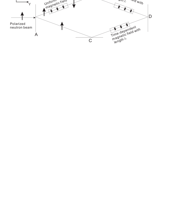
Figure 1: Schematic experimental setup for measuring the QGP.

The proposed experimental setup is shown in Fig. (1). A polarized-spin-up($\left|{+z}\right\rangle$) neutron beam splits into two beams at the position $(y=0,z=0)$ of interface $A$ due to Laue scattering. Before the upper beam is reflected, a uniform magnetic field is placed in the neutron propagation path of upper beam, which rotates the spin up to spin down($\left|{-z}\right\rangle$). Two time-dependent magnetic fields are applied to the system after the two beams are reflected. The beginning locations of the two fields are both at $(y_{0},\pm z_{0})$, and the two fields have the same time-dependence. Since $|{\bf p}|$ (${\bf p}$ is the momentum of the neutron beams) is the same between the upper and lower beams during the propagation, thus two beams will arrive at the time-dependent magnetic fields at the same time $t_{0}$, which should be able to precisely controlled in the experiment.

At $t_{0}$ we turn on the time-dependent magnetic field with the initial condition that $\left|{+z}\right\rangle$ and $\left|{-z}\right\rangle$ as the eigenstates of the Hamiltonian. The lengths of time-dependent magnetic fields in upper and lower paths are $l_{1}$ and $l_{2}$. For measuring the quantum geometric potential, the two lengths are different in general, without loss of generality we set $l_{2}>l_{1}$, then the upper and lower-branch of neutrons will experience different evolution time with the same time-dependent magnetic fields. The sufficient quantum adiabatic condition (similar as the qualitative condition of Eq. (6)) derived in Ref.Wu et al. (2008) needs to be imposed for guaranteeing the time evolutions of the two neutron beams to be quantum adiabatic. Finally the two neutron beams meet at destination $D$. By measuring neutron spin coherent information at location $D$, we can get both fo the information of the QGP and the $U(1)$-invariant basis (Eq. (4)).

Suppose now everything is under well control, then after the neutrons fly through the time-dependent magnetic field in the upper path, the final state of neutron becomes (assuming taking $t_{1}$ time for passing through that region)

$$\left|{\Phi_{-}^{adia}(t_{1})}\right\rangle=\exp\left\{{-i\int_{0}^{t_{1}}{\left[{e_{-}(\lambda)-\mathcal{A}_{-}(\lambda)}\right]d\lambda}}\right\}\left|{\varphi_{-}(t_{1})}\right\rangle$$ (9)

For the other path the final state becomes,

$$\left|{\Phi_{+}^{adia}(t_{2})}\right\rangle=\exp\left\{{-i\int_{0}^{t_{2}}{\left[{e_{+}(\lambda)-\mathcal{A}_{+}(\lambda)}\right]d\lambda}}\right\}\left|{\varphi_{+}(t_{2})}\right\rangle$$ (10)

As a result, their coherent intensity at point $D$ follows by

$$I(t_{1},t_{2})=\frac{1}{2}\left|{\left|{\Phi_{-}^{adia}(t_{1})}\right\rangle+\left|{\Phi_{+}^{adia}(t_{2})}\right\rangle}\right|^{2}=1+\frac{1}{2}\left\langle{{\Phi_{-}^{adia}(t_{1})}}\mathrel{\left|{\vphantom{{\Phi_{-}^{adia}(t_{1})}{\Phi_{+}^{adia}(t_{2})}}}\right.\kern-1.2pt}{{\Phi_{+}^{adia}(t_{2})}}\right\rangle+\frac{1}{2}\left\langle{{\Phi_{+}^{adia}(t_{2})}}\mathrel{\left|{\vphantom{{\Phi_{+}^{adia}(t_{2})}{\Phi_{-}^{adia}(t_{1})}}}\right.\kern-1.2pt}{{\Phi_{-}^{adia}(t_{1})}}\right\rangle$$

$$= 1+\frac{1}{2}\left({\exp\left\{{i\int_{0}^{t_{1}}{\left[{e_{-}(\lambda)-\mathcal{A}_{-}(\lambda)}\right]d\lambda}}\right\}\exp\left\{{-i\int_{0}^{t_{2}}{\left[{e_{+}(\lambda)-\mathcal{A}_{+}(\lambda)}\right]d\lambda}}\right\}\left\langle{{\varphi_{-}(t_{1})}}\mathrel{\left|{\vphantom{{\varphi_{-}(t_{1})}{\varphi_{+}(t_{2})}}}\right.\kern-1.2pt}{{\varphi_{+}(t_{2})}}\right\rangle+c.c}\right)$$

$$= 1+\frac{1}{2}\left({\exp\left\{{i\int_{0}^{t_{1}}{e_{-}(\lambda)d\lambda}-i\int_{0}^{t_{2}}{e_{+}(\lambda)d\lambda}}\right\}}\right.\left.{\exp\left\{{-i\int_{0}^{t_{1}}{\mathcal{A}_{-}(\lambda)d\lambda}+i\int_{0}^{t_{2}}{\mathcal{A}_{+}(\lambda)d\lambda}}\right\}\left\langle{{\varphi_{-}(t_{1})}}\mathrel{\left|{\vphantom{{\varphi_{-}(t_{1})}{\varphi_{+}(t_{2})}}}\right.\kern-1.2pt}{{\varphi_{+}(t_{2})}}\right\rangle+c.c}\right),$$

(11)

where $c.c$ is used to denote the conjugate term. Now fine tuning $l_{2}$ for letting the length of $l_{2}$ just slightly larger than the $l_{1}$, i.e., $l_{2}=l_{1}+\delta l$, then $t_{2}=t_{1}+\delta t$. Substituting this back to the coherent intensity of Eq. (11), we obtain (noting the fact that $I(t_{1},t_{1})=1$),

$$2(I(t_{1},t_{1}+\delta t)-I(t_{1},t_{1}))=\left({\cos\left[{\int_{0}^{t_{1}}{\left[{e_{-}(\lambda)-e_{+}(\lambda)+\Delta_{+-}(\lambda)}\right]d\lambda}}\right]}\right)\left|{\langle\varphi_{-}|\dot{\varphi}_{+}\rangle}\right|\delta t+O\left({(\delta t)^{2}}\right)$$ (12)

$\Rightarrow$

$$\left.{\frac{{\partial I(t_{1},t_{2})}}{{\partial t_{2}}}}\right|_{t_{2}\to t_{1}}=\mathop{\lim}\limits_{\delta t\to 0}\frac{{I(t_{1},t_{1}+\delta t)-I(t_{1},t_{1})}}{{\delta t}}=\frac{1}{2}\left|{\langle\varphi_{-}|\dot{\varphi}_{+}\rangle}\right|\cos\left[{\int_{0}^{t_{1}}{\left[{e_{-}(\lambda)-e_{+}(\lambda)+\Delta_{+-}(\lambda)}\right]d\lambda}}\right].$$ (13)

From Eq. (13), as expected, the oscillation of the coherent density is not longer solely determined by the instantaneous energy gap but also modified by the QGP. By measuring the differential coherent density, after subtracting out the phase contribution from the dynamic part from the instantaneous energy gap, we can directly verify the existence of the QGP — the quantum “geodesic curvature” of any two sub-manifolds with two different instantaneous eigenstates in time-dependent Hamiltonian. It is worth to note that when the time-evolution completes a cycle in Eq. (13), the proposal can also help probe the influence of the quantized character originating from the QGP [Eq. (7)]. The spirit of the proposal in neutron experiment can be equivalently converted to other type of experimental platforms, as well as applied to generic parameterized quantum systems. Now let’s move to an explicit model which can be realized by real experiments.

An explicit experimental accessible model. —

Consider following spin-$\frac{1}{2}$ particle in a rotating magnetic field. The Hamiltonian of the system is

$$h(\tau)=\eta\sigma_{z}+\xi\left[{\sigma_{x}\cos(2K\eta\tau)+\sigma_{y}\sin(2K\eta\tau)}\right]$$ (14)

with time-independent eigenvalues $E_{\pm}=\pm\sqrt{\eta^{2}+\xi^{2}}$. Properly choosing phases, two adiabatic orbits (instantaneous eigenstates) can be expressed as

$$\left|{\varphi_{+}(\tau)}\right\rangle=\cos(\theta/2)\left|0\right\rangle+e^{2iK\eta\tau}\sin(\theta/2)\left|1\right\rangle$$ (15)

$$\left|{\varphi_{-}(\tau)}\right\rangle=\sin(\theta/2)\left|0\right\rangle-e^{2iK\eta\tau}\cos(\theta/2)\left|1\right\rangle$$ (16)

where $\cos\theta=\eta/\sqrt{\eta^{2}+\xi^{2}}$. It is straightforward to obtain $\Delta_{+-}=2K\eta\cos\theta$ and $|{\langle\varphi_{-}|\dot{\varphi}_{+}\rangle}|=|K\eta\sin\theta|$ $=|K\eta\xi/\sqrt{\eta^{2}+\xi^{2}}|$, both are time-independent in this simple model.

Now let’s set parameters on neutron, $\eta\sim$ 500 Gauss$\times$$\mu_{n}$ (${\rm{neutron\;magneton}}\;\mu_{n}=-1.913\times{\rm nuclear\;magneton}=5.05\times 10^{-27}J/{\rm Tesla}=9.66\times 10^{-27}J/{\rm Tesla}$) and $\xi\sim 5$ Gauss$\times$$\mu_{n}$, whose corresponding energy scales are $\eta\sim 4.78\times 10^{-28}J\sim 721$KHz and $\xi\sim 7.21$KHz. Then if we choose $K=5$, then the rotation frequency on the $x$-$y$ plane is around $7.21$MHz which is doable under current experimental conditions. Furthermore we have $\cos\theta\approx 0.99995$ which indicates $\theta$ is almost zero which are well consistent with initial condition. With those chosen parameters, it is easy to verify that $|{\langle\varphi_{-}|\dot{\varphi}_{+}\rangle}|/|E_{-}-E_{+}-\Delta_{+-}|=K/(2(\xi/\eta+\eta/\xi)+2K\eta/\xi)<5/1000\ll 1$ which satisfies the sufficient adiabatic condition derived in Ref. Wu et al. (2008) with the fidelity $F>99/100$. This indicates the system’s time evolution can be well described by the quantum adiabatic evolution. Since $\Delta_{+-}=2K\eta\cos\theta\approx 10\eta$ and $E_{-}-E_{+}\approx-2\eta$, so under this set of parameters one should observe the behavior of $dI/dt\propto\cos(8\eta\tau)$ with an oscillation frequency of around 5.77MHz, about four times of the (instantaneous) energy gap. Thus with the chosen parameters the QGP has much more contribution than that of the energy gap of the system, which should be easily identified in the experiments. If the $z$-direction coupling is removed in the above Hamiltonian, then the effects of QGP disappears, the system’s dynamics will be governed by the energy gap of the system. Actually if the oscillation of magnetic field along $z$-direction is further turned on, one can have a better proposal, whose details will be deferred to a future publication.

Discussions and conclusions. —

At first glance one may think the QGP as a certain transforming form of the Berry curvatureXiao et al. (2010) since both of them are induced by the Berry connection in certain ways, however, they are complementary. In any instantaneous eigenstate, the $n^{th}$ instantaneous orbital in the Hilbert space $\left|{\varphi_{n}(\tau)}\right\rangle$ of a system, all of its parameters compose a sub-manifold (consider the total Hamiltonian composed by all instantaneous eigenvalues and eigenstates as a total manifold). Along its time evolution direction, the Berry curvature (Eq. (8)) is defined in the corresponding sub-manifold classified by the quantum number $n$. As a result, the Berry curvature is locally defined and solely lives in a $n^{th}$ manifold. The difference now becomes crystal clear, although QGP is also a local-gauge invariant term, but the more important fact is that the QGP relates any two sub-manifolds characterized by two different quantum numbers during the time-dependent evolution. The difference is manifest when considering a single spin-$\frac{1}{2}$ coupled to a general time-dependent magnetic field, $H=B{\bf{\sigma}}\cdot{\bf{n}}(\tau)$ with the magnetic moment absorbed into the magnetic field $B$, and the unit vector $\bf{n}(\tau)=(\sin\theta(\tau)\cos\phi(\tau),\sin\theta(\tau)\sin\phi(\tau),\cos\theta(\tau))$ denotes the direction of the field. Its Berry curvature becomes $\sin\theta/2$ (corresponding to the sub-manifold with eigenvalue $B$), while the corresponding QGP follows by,

$$\Delta_{+-}=\frac{{\dot{\theta}\ddot{\phi}\sin\theta+2\dot{\theta}^{2}\dot{\phi}\cos\theta+\dot{\phi}^{3}\sin^{2}\theta\cos\theta-\dot{\phi}\ddot{\theta}\sin\theta}}{{\dot{\theta}^{2}+(\dot{\phi}\sin\theta)^{2}}},$$ (17)

which is equal to the geodesic curvature of the unit 2-sphere multiplied with the 2-sphere measure distance $(\dot{\theta}^{2}+(\dot{\phi}\sin\theta)^{2})^{1/2}$ Wu et al. (2008).

Once the QGP is restricted into only one sub-manifold, say $n=m$, the QGP just disappears. In this sense the QGP is a physical quantity reflecting important geometric characteristics between different sub-manifolds in the generic parameterized quantum system. The emergence of the Berry phase implies that one can not fix the phase factor globally during the time evolution. The QGP further indicates that even locally at any instant moment the phase factor can not be fixed arbitrarily either. The two quantities are complimentary between each other, laying down a better and more complete picture for understanding the geometric characteristics and even the topology in the time-dependent and generic parameterized quantum systems.

In summary, we propose a straightforward interference measurement to directly probe the QGP, following which a measurement on the influence of the corresponding quantized character is also possible after a cyclic time-evolution. It is expected that the proposal can be carried out by certain experiments in the near future. The physical and geometric implications of the QGP are also discussed and analysed following the simple spin-$\frac{1}{2}$ model. Based on the unique features of the Berry phase and the QGP, we conclude that the two quantities are complementary.

References

- Born and Fock (1928) M. Born and V. Fock, Zeitschrift für Physik A Hadrons and Nuclei 51, 165 (1928).
- Schwinger (1937) J. Schwinger, Phys. Rev. 51, 648 (1937).
- Kato (1950) T. Kato, J. Phys. Soc. of Japan 5, 435 (1950).
- Landau (1932) L. Landau, Phys. Z. Sowjetunion 2, 7 (1932).
- Zener (1932) C. Zener, in Proceedings of the Royal Society of London A: Mathematical, Physical and Engineering Sciences (The Royal Society, 1932), vol. 137, pp. 696–702.
- Gell-Mann and Low (1951) M. Gell-Mann and F. Low, Phys. Rev. 84, 350 (1951).
- Berry (1984) M. Berry, Phys. Eng. Sci. 392, 45 (1984).
- Simon (1983) B. Simon, Phys. Rev. Lett. 51, 2167 (1983).
- Oreg et al. (1984) J. Oreg, F. Hioe, and J. Eberly, Phys. Rev. A 29, 690 (1984).
- Schiemann et al. (1993) S. Schiemann, A. Kuhn, S. Steuerwald, and K. Bergmann, Phys. Rev. Lett. 71, 3637 (1993).
- Pillet et al. (1993) P. Pillet, C. Valentin, R.-L. Yuan, and J. Yu, Phys. Rev. A 48, 845 (1993).
- Jones et al. (2000) J. A. Jones, V. Vedral, A. Ekert, and G. Castagnoli, Nature 403, 869 (2000).
- Farhi et al. (2001) E. Farhi, J. Goldstone, S. Gutmann, J. Lapan, A. Lundgren, and D. Preda, Science 292, 472 (2001).
- Childs et al. (2001) A. M. Childs, E. Farhi, and J. Preskill, Phys. Rev. A 65, 012322 (2001).
- Zheng (2005) S.-B. Zheng, Phys. Rev. Lett. 95, 080502 (2005).
- Ashhab et al. (2006) S. Ashhab, J. Johansson, and F. Nori, Phys. Rev. A 74, 052330 (2006).
- Das and Chakrabarti (2008) A. Das and B. K. Chakrabarti, Rev. Mod. Phys. 80, 1061 (2008).
- Rezakhani et al. (2009) A. Rezakhani, W.-J. Kuo, A. Hamma, D. Lidar, and P. Zanardi, Phys. Rev. Lett. 103, 080502 (2009).
- Bason et al. (2012) M. G. Bason, M. Viteau, N. Malossi, P. Huillery, E. Arimondo, D. Ciampini, R. Fazio, V. Giovannetti, R. Mannella, and O. Morsch, Nat. Phys. 8, 147 (2012).
- Georgescu et al. (2014) I. Georgescu, S. Ashhab, and F. Nori, Rev. Mod. Phys. 86, 153 (2014).
- Albash and Lidar (2016) T. Albash and D. A. Lidar, arXiv:1611.04471 (2016).
- Santos and Sarandy (2017) A. C. Santos and M. S. Sarandy, arXiv:1702.02239 (2017).
- Xiao et al. (2010) D. Xiao, M.-C. Chang, and Q. Niu, Rev. Mod. Phys. 82, 1959 (2010).
- Eckardt (2017) A. Eckardt, Rev. Mod. Phys. 89, 011004 (2017).
- Niu (1990) Q. Niu, Phys. Rev. Lett. 64, 1812 (1990).
- Thouless (1983) D. J. Thouless, Phys. Rev. B 27, 6083 (1983).
- Murakami et al. (2003) S. Murakami, N. Nagaosa, and S.-C. Zhang, Science 301 (2003).
- Murakami et al. (2004) S. Murakami, N. Nagosa, and S.-C. Zhang, Phys. Rev. B 69, 235206 (2004).
- Guo et al. (2008) G.-Y. Guo, S. Murakami, T.-W. Chen, and N. Nagaosa, Phys. Rev. Lett. 100, 096401 (2008).
- Haldane (1988) F. D. M. Haldane, Phys. Rev. Lett. 61, 2015 (1988).
- Aidelsburger et al. (2011) M. Aidelsburger, M. Atala, S. Nascimbène, S. Trotzky, Y.-A. Chen, and I. Bloch, Phys. Rev. Lett. 107, 255301 (2011).
- Heyl (2015) M. Heyl, Phys. Rev. Lett. 115, 140602 (2015).
- Jotzu et al. (2014) G. Jotzu, M. Messer, R. Desbuquois, M. Lebrat, T. Uehlinger, D. Greif, and T. Esslinger, Nature 515, 237 (2014).
- Wilczek and Zee (1984) F. Wilczek and A. Zee, Phys. Rev. Lett. 52, 2111 (1984).
- Wilson (1974) K. G. Wilson, Phys. Rev. D 10, 2445 (1974).
- Wu et al. (2008) J. Wu, M. Zhao, J. Chen, and Y. Zhang, Phys. Rev. A 77, 062114 (2008).
- Du et al. (2008) J. Du, L. Hu, Y. Wang, J. Wu, M. Zhao, and D. Suter, Physical review letters 101, 060403 (2008).
- Xu et al. (2017) C. Xu, J. Wu, and C. Wu, arXiv:1712.00082 (2017).
- Zhang (2010) Y. Zhang, Advanced Quantum Mechanics, Second Edition (Science Press, China, 2010).
- Zhao and Wu (2011) M. Zhao and J. Wu, Phys. Rev. Lett. 106, 138901 (2011).