Uniaxial and biaxial structures in the elastic Maier-Saupe model

Abstract

We perform statistical mechanics calculations to analyze the global phase diagram of a fully-connected version of a Maier-Saupe-Zwanzig lattice model with the inclusion of couplings to an elastic strain field. We point out the presence of uniaxial and biaxial nematic structures, depending on temperature $T$ and on the applied stress $\sigma$. Under uniaxial extensive tension, applied stress favors uniaxial orientation, and we obtain a first-order boundary, along which there is a coexistence of two uniaxial paranematic phases, and which ends at a simple critical point. Under uniaxial compressive tension, stress favors biaxial orientation; for small values of the coupling parameters, the first-order boundary ends at a tricritical point, beyond which there is a continuous transition between a paranematic and a biaxially ordered structure. For some representative choices of the model parameters, we obtain a number of analytic results, including the location of critical and tricritical points and the line of stability of the biaxial phase.

I Introduction

Nematic elastomers are an interesting class of soft-matter systems, with an interplay of the effects of nematic order and of elastic properties of rubber materials Warner2003 . At fixed and sufficiently low temperatures, elastomer systems display stress-strain curves with a plateau that resembles a liquid-gas transition. Since the pioneering work of de Gennes and collaborators deGennes1975 ; deGennesProst1993 ; deGennesOkumura2003 , the couplings between elastic and orientational degrees of freedom have been recognized as the essential ingredient to account for the behavior of elastomers. More recently, it has been argued that it is also important to introduce quenched random fields, which are supposed to smooth the first-order transition, and which are related to the phase history of the cross-links of the polymer network Fridrikh1997 ; Yu1998 ; Selinger2002 ; Selinger2004 ; Fridrich2006 ; Petridis2006 ; Zhu2011 . In a recent work, some of us performed mean-field calculations for a basic Maier-Saupe lattice model, which was supplemented by the addition of an elastic strain field and of random fields Liarte2011 ; Liarte2013 . At the qualitative level, it has been possible to account for many of the experimental properties of uniaxial nematic elastomers. We were then motivated to revisit this elementary lattice model, with the addition of a simple form of elastic coupling, and with no random fields. The fully-connected version of this model system, as we define in Section 2, is amenable to detailed and standard statistical mechanics calculations doCarmo2011 ; Liarte2014 . We show that the introduction of a coupling to an external strain field is sufficient to provide a mechanism to change and depress the standard first-order nematic transition, and make contact with the plateaux in the stress-strain curves of nematic elastomers. In Section 3, we obtain a number of analytic results for the stress-temperature phase diagram of some simple representative cases. We show the existence of a rich behavior, including critical and tricritical points and the continuous transition to a biaxial nematic structure.

As in the original phenomenological treatment of de Gennes and collaborators deGennesOkumura2003 , the external stress in the elastic nematic model system plays a similar role as an applied magnetic (electric) field in the corresponding uniaxial nematic system. A magnetic field couples to the nematic order via a constant $\chi_{a}$ that can be either positive or negative deGennesProst1993 . Positive values of this susceptibility ($\chi_{a}>0$) correspond to positive tensions (extension) in the elastic model. In the phase diagrams, either in terms of stress or in terms of fields and temperature, there is a line of first-order transitions that ends at a simple critical point Petri2016 . Negative values of the susceptibility ($\chi_{a}<0$) lead to a field-induced biaxial phase.

It is interesting to remark that Ye, Lubensky and coworkers have considered a minimal model Ye2007 ; Ye2009 , at the phenomenological level, which provides a robust description of the elastic semisoft response of nematic elastomers. In addition to the uniaxial strain field, these authors also add a transverse strain component, which might as well be produced in the cross-linking Küpfer-Finkelmann procedure of preparing elastomer samples Kuepfer1991 . They point out that this minimal model is analogous to the formulation of a nematic system in the presence of crossed electric and magnetic field, which also leads to a rich phase diagram, with critical and tricritical behavior, and the possibility of existence of a biaxial phase. In the present work, however, we consider a minimal lattice model, and keep the restriction to an elastic strain field along the uniaxial direction.

In the elastic model of the present work, negative tensions (compression) may lead to a stress-induced biaxial phase. In figure 1a, for sufficiently weak and typical values of the coupling parameters, we draw a sketch of a representative phase diagram of a uniaxial nematic system in terms of applied stress (along the uniaxial direction) and temperature. For larger values of the coupling parameters, the tricritical point collapses at the first-order boundary, and the topology of this diagram may be drastically changed (figure 1b).

(a)

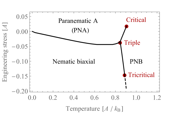
(b)

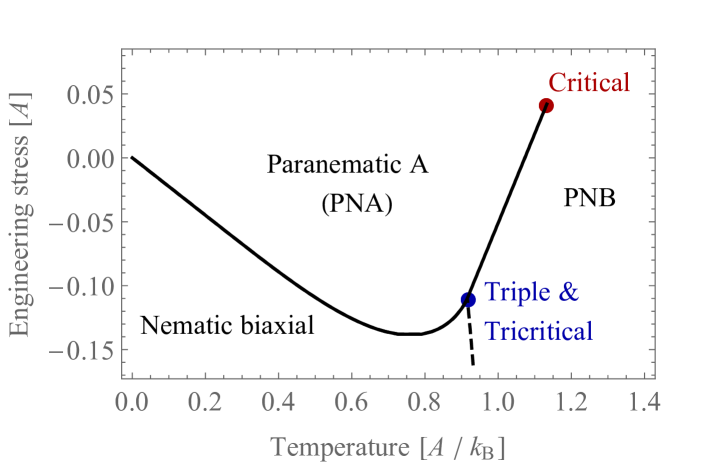
Figure 1: Sketch of the stress-temperature phase diagram of a uniaxial nematic system for small (a) and large (b) values of the coupling parameters. Solid and dashed lines correspond to first and second-order transitions. We indicate critical and tricritical points.

II The elastic Maier-Saupe model

In the Maier-Saupe approach to the nematic transitions, we consider a lattice of $N$ sites and write the energy

$$\mathcal{H}_{MS}=-A\sum_{\left(i,j\right)}\sum_{\mu,\nu=x,y,z}S_{i}^{\mu\nu}S_{j}^{\mu\nu},$$ (1)

where $A>0$ is an interaction parameter, the first sum is over nearest-neighbor pairs of lattice sites, and the local “quadrupolar” degrees of freedom are given by

$$S_{i}^{\mu\nu}=\frac{1}{2}\left(3n_{i}^{\mu}n_{i}^{\nu}-\delta_{\mu\nu}\right),$$ (2)

where $\overrightarrow{n}_{i}$ is the unit director associated with a nematogenic molecule at site $i=1,2,...,N$, and $\delta_{\mu\nu}$ is the Kronecker delta.

In the mean-field calculations of this work, we assume a fully-connected version of this Maier-Saupe model, given by the energy

$$E_{MS}=-\frac{A}{N}\sum_{1\leq i<j\leq N}\sum_{\mu,\nu=x,y,z}S_{i}^{\mu\nu}S_{j}^{\mu\nu},$$ (3)

where the first sum is over all pairs of lattice sites, and the parameter $A$ is suitably scaled to preserve the existence of the thermodynamic limit. We further assume that the local directors $\overrightarrow{n}_{i}$ are restricted to the Cartesian axes,

$$\overrightarrow{n}_{i}=\left\{\begin{array}[c]{c}\left(\pm 1,0,0\right),\\ \left(0,\pm 1,0\right),\\ \left(0,0,\pm 1\right),\end{array}\right.$$ (4)

which leads to a three-state statistical model. This choice of discrete orientational degrees of freedom, which resembles an approximation used by Zwanzig to treat the Onsager model for the nematic transition, leads to a problem that is amenable to quite simple statistical-mechanics calculations (and to simple simulations as well). Moreover, it is known that this elementary MSZ model leads to essentially the same qualitative results as obtained from slightly more involved calculations for the original Maier-Saupe model with a continuous distribution of orientational degrees of freedom Liarte2014 ; Nascimento2016 . We should keep in mind, however, that the continuous symmetry may be strictly necessary to describe some special features of these systems, as the soft transitions observed in liquid-crystal elastomers Liarte2013 . It is possible that the soft/semisoft response of nematic elastomers depletes the biaxial nematic state.

According to the notation of our previous article Liarte2011 , the energy of a microscopic configuration of the elastic Maier-Saupe lattice model is written as a sum of three terms,

$$E=E_{MS}+E_{elastic}+E_{coupling},$$ (5)

where $E_{MS}$ is given by eq. (3). Here we ignore the quenched random fields originating in the aligning stresses that are generated at the time of cross-linking. Hence, positive stresses lead to a nematic director that is aligned with the axis of deformation.

The theory of rubber elasticity, as developed by Warner and Terentjev Warner2003 , leads to the elastic free energy per site of a lattice polymer,

$$f_{rub}=\frac{1}{2}\mu_{s}\left(\lambda^{2}+\frac{2}{\lambda}\right),$$ (6)

where $\mu_{s}>0$ is a linear shear modulus and $\lambda$ is the distortion factor of a uniaxial, volume-preserving, deformation. In order to keep the calculations as simple as possible, and restrict the analysis to an elementary model that is still capable of qualitatively accounting for the effects of strain, we expand $f_{rub}$ about the minimum, $\lambda=1$, and keep quadratic terms only. We then discard an additive term, $\left(3/2\right)\mu_{s}N$, and write the elastic energy,

$$E_{elastic}=\frac{3}{2}\mu_{s}N\left(\lambda-1\right)^{2}.$$ (7)

We now discuss the couplings between orientational degrees of freedom and a uniform external strain along a certain direction. According to previous work Liarte2011 , we introduce a global tensor,

$$M_{\mu\nu}=\frac{1}{2}\left(3m^{\mu}m^{\nu}-\delta_{\mu\nu}\right),$$ (8)

which characterizes a global uniaxial deformation, where the stress is applied along the unit vector $\overrightarrow{m}$ (which is distinct from the local nematic directors). If we use the Warner-Terentjev theory Warner2003 , and keep the dominant contribution near the minimum $\lambda=1$, the coupling term of the energy is written as

$$E_{coupling}=-B\sum_{i=1}^{N}\sum_{\mu,\nu}M_{\mu\nu}S_{i}^{\mu\nu},$$ (9)

with

$$B=\mu_{s}\delta\left(\lambda-1\right),$$ (10)

where the parameter $\delta$ gauges the strain anisotropy (and is usually assumed to be positive).

We emphasize that rubber elasticity is a primarily entropic phenomenon. Polymer chains optimally arrange themselves according to high-entropy configurations instead of configurations that lower an interatomic or molecular potential. Therefore, the elastic and coupling terms in equation (5) come from a degeneracy factor associated with the configurations of the polymer network, and should be regarded as effective energy terms Liarte2011 ; Liarte2013 . Also, the linear chain modulus is usually taken as proportional to temperature, so in this work we assume that

$$\mu_{s}=n_{s}k_{B}T,$$ (11)

where $T$ is the temperature, $k_{B}$ is the Boltzmann constant, and $n_{s}$ is the relative number of polymer strands.

The thermodynamic properties of this elastic MSZ model can be obtained from a canonical partition function in the stress ensemble, which is given by

$$Y=Y\left(T,\sigma,N,\left\{M_{\mu\nu}\right\}\right)=\int d\lambda\exp\left[N\beta\sigma\lambda\right]\times$$

$$\times\sum_{\left\{\overrightarrow{n}_{i}\right\}}\exp\left[-\beta\left(E_{MS}+E_{elastic}+E_{coupling}\right)\right],$$ (12)

where $\beta=1/k_{B}T$, $\sigma$ is the global engineering stress, and the sum is over all configurations of the local nematic directors. Taking into account equations (3), (7), and (9), and discarding irrelevant terms in the thermodynamic limit, we write

$$Y =\int d\lambda\exp\left[N\beta\sigma-\frac{3}{2}N\beta\mu_{s}-\frac{3}{2}N\beta\mu_{s}\,\left(\lambda-1\right)^{2}\right]$$

$$\quad\times\sum_{\left\{\overrightarrow{n}_{i}\right\}}\exp\left[-\beta E_{eff}\right],$$ (13)

with

$$E_{eff}=-\frac{A}{2N}\sum_{\mu,\nu}\left(\sum_{i=1}^{N}S_{i}^{\mu\nu}\right)^{2}-B\sum_{i=1}^{N}\sum_{\mu,\nu}M_{\mu\nu}S_{i}^{\mu\nu},$$ (14)

where $A>0$ is a constant dimensional parameter, and the expression of $B$ is given by eqs. (10) and (11),

$$B=n_{s}k_{B}T\delta\left(\lambda-1\right).$$ (15)

We now resort to well-known techniques of statistical mechanics. If we use a set of Gaussian identities to deal with the quadratic terms, and change to more convenient variables, it is straightforward to write

$$\sum_{\left\{\overrightarrow{n}_{i}\right\}}\exp\left[-\beta E_{eff}\right]=\int\left[dQ_{\mu\nu}\right]$$

$$\quad\times\exp\left[-\sum_{\mu,\nu}\frac{\beta AN}{2}Q_{\mu\nu}^{2}\right]\,\left(Z_{1}\right)^{N},$$ (16)

with the short-hand notation

$$\int\left[dQ_{\mu\nu}\right]\left(...\right)={\displaystyle\prod\limits_{\mu,\nu}}\int\left(\frac{\beta AN}{2\pi}\right)^{1/2}dQ_{\mu\nu}\left(...\right),$$ (17)

where $Z_{1}$ is a single-particle partition function,

$$Z_{1}=\sum_{\overrightarrow{n}}\exp\left\{\beta\sum_{\mu,\nu}\left[AQ_{\mu\nu}+BM_{\mu\nu}\right]S_{\mu\nu}\right\}.$$ (18)

Performing the sum over the nematic directors according to the six possibilities of eq. (4), we finally have

$$Z_{1} =2\exp\left[-\frac{\beta A}{2}\sum_{\mu}Q_{\mu\mu}\right]\sum_{\mu}\exp\left[\frac{3}{2}\beta AQ_{\mu\mu}\right.$$

$$\quad\left.+\frac{3}{2}\beta BM_{\mu\mu}\right].$$ (19)

We now use these expressions to write

$$Y=\int d\lambda\int\left[dQ_{\mu\nu}\right]\exp\left[-\beta Ng_{f}\right],$$ (20)

where the free-energy functional is given by

$$g_{f} =-\sigma\lambda+\frac{3}{2}\mu_{s}+\frac{3}{2}\mu_{s}\left(\lambda-1\right)^{2}+\frac{1}{2}A\sum_{\mu,\nu}Q_{\mu\nu}^{2}$$

$$\quad+\frac{1}{2}A\sum_{\mu}Q_{\mu\mu}-\frac{1}{\beta}\ln 2-\frac{1}{\beta}\ln\left\{\sum_{\mu}\right.$$

$$\quad\left.\exp\left[\frac{3}{2}\beta AQ_{\mu\mu}+\frac{3}{2}\beta BM_{\mu\mu}\right]\right\}.$$ (21)

It should be remarked that $g_{f}$ is a function of temperature $T$, global external stress $\sigma$, and the components of the tensor $M_{\mu\nu}$, as well as of the strain distortion $\lambda$ and the components of the tensor order parameter $Q_{\mu\nu}$. The thermodynamic free energy per site, $g=g\left(T,\sigma\right)$, comes from a saddle-point calculation, which amounts to a minimization of $g_{f}$ with respect to $\lambda$ and $\left\{Q_{\mu\nu}\right\}$,

$$g=g\left(T,\sigma\right)=\min\limits_{\lambda,\left\{Q_{\mu\nu}\right\}}g_{f}\left(T,\sigma;\lambda,\left\{Q_{\mu\nu}\right\}\right).$$ (22)

From the saddle-point equations, we have

$$Q_{\mu\mu}=\frac{1}{2}\left(\frac{3e_{\mu}}{\sum_{\nu}e_{\nu}}-1\right),$$ (23)

where

$$e_{\mu}=\exp\left[\frac{3}{2}\beta AQ_{\mu\mu}+\frac{9}{4}\beta Bm_{\mu}^{2}\right],$$ (24)

and $m_{\mu}$ is a component of the unit vector $\overrightarrow{m}$ associated with the global tensor $M_{\mu\nu}$. It is easy to see that $Q_{\mu\nu}=0$ for $\mu\neq\nu$, and that $Q_{\mu\nu}$ is a traceless tensor,

$$\sum_{\mu}Q_{\mu\mu}=0.$$ (25)

The derivative with respect to $\lambda$ leads to the remaining saddle-point equation,

$$-\frac{\sigma}{\mu_{s}}+3\left(\lambda-1\right)-\frac{3}{2}\delta\sum_{\mu}m_{\mu}^{2}\,Q_{\mu\mu}=0.$$ (26)

At this point the problem is formulated in quite general terms. We use equations (23) and (26) for obtaining the nematic order parameter $Q_{\mu\mu}$ and the distortion $\lambda$ in terms of temperature $T$, external stress $\sigma$, global strain $M_{\mu\nu}$, and the parameters of the model. If there are multiple solutions, we have to search for the absolute minima of the functional $g_{f}\left(T,\sigma,\left\{M_{\mu\nu}\right\};\,\lambda,\left\{Q_{\mu\nu}\right\}\right)$. Several choices of parameters and particular cases can be analyzed rather easily.

III Calculations for some special cases

We now use the standard representation of the nematic tensor order parameter,

$$\mathbf{Q}=\left(\begin{array}[c]{ccc}-\frac{1}{2}\left(S+\eta\right)&0&0\\ 0&-\frac{1}{2}\left(S-\eta\right)&0\\ 0&0&+S\end{array}\right).$$ (27)

Also, we assume that the global external strain is applied along the $z$ direction,

$$\overrightarrow{m}=\left(0,0,1\right).$$ (28)

From the saddle-point equations, (23) and (26), it is straightforward to write the mean-field equations of state

$$S=1-\frac{3}{2+\exp{\left(9\,\beta\,(B+S)/4\right)}\,\text{sech}(3\,\beta\,\eta/4)},$$ (29)

$$\eta=\frac{3\,\tanh\left(3\,\beta\,\eta/4\right)}{2+\exp{\left(9\,\beta\,(B+S)/4\right)}\,\text{sech}\left(3\,\beta\,\eta/4\right)},$$ (30)

and

$$\frac{\sigma}{\mu_{s}}=3\left(\lambda-1\right)-\frac{3}{2}\delta S,$$ (31)

where $B$ is given by equation (15), and we are setting $A=1$ to simplify the notation. The free energy functional can be written as

$$g_{f} =-\sigma\lambda+\frac{3}{2}\mu_{s}+\frac{3}{2}\mu_{s}\left(\lambda-1\right)^{2}+\frac{1}{2}\left(\frac{3}{2}S^{2}+\frac{1}{2}\eta^{2}\right)$$

$$\quad-\frac{1}{\beta}\ln 2+\frac{3}{4}\mu_{s}\delta\left(\lambda-1\right)--\frac{1}{\beta}\ln\left[2\exp\left(-\frac{3}{4}\beta S\right)\right.$$

$$\quad\left.\times\cosh\left(\frac{3}{4}\beta\eta\right)+\exp\left(\frac{3}{2}\beta S+\frac{9}{4}\beta B\right)\right].$$ (32)

From equation (31), we have

$$\left(\lambda-1\right)=\frac{\sigma}{3\mu_{s}}+\frac{1}{2}\delta S.$$ (33)

Therefore, the coupling parameter $B$ to the strain field is given by

$$B=\mu_{s}\delta\left(\lambda-1\right)=\frac{1}{3}\sigma\delta+\frac{1}{2}\mu_{s}\delta^{2}S,$$ (34)

so that the strength of this coupling depends on the stress. For $\delta>0$ and $\sigma$ sufficiently large, the system prefers to align uniaxially (there is a stable uniaxial solution, $S\neq 0$ and $\eta=0$). For negative and sufficiently large values of the stress $\sigma$, with positive strain anisotropy, $\delta>0$, we anticipate the possibility of a biaxial arrangement ($S\neq 0$ and $\eta\neq 0$).

III.1 Uniaxial transitions

In zero stress, $\sigma=0$, we have $B=\mu_{s}\delta^{2}S/2$, so that $S=0$ (with $\eta=0$) is a solution of the saddle point equations. At low temperatures, however, this fully disordered solution is unstable, and there appears a thermodynamic stable, uniaxially ordered solution, $S\neq 0$ and $\eta=0$. For $\sigma\neq 0$, however, the solution $S=0$ is no longer acceptable.

In the stress-temperature phase diagram, assuming $\delta>0$, we anticipate the existence of a line of coexistence of two distinct and uniaxially ordered phases. Along this first-order line, as the temperature increases, there is a decrease of the difference $\Delta S$ between the scalar order parameters associated with the coexisting phases, which finally vanishes at a simple critical point. This depression of $\Delta S$ is one of the hallmarks of the behavior of elastomers Warner2003 . Given the parameters of the model, we can draw a number of graphs of the solution $S$ versus temperature $T$ for various values of the external stress $\sigma$ (see figures in the article by Liarte, Yokoi, and Salinas Liarte2011 ). Also, we can draw graphs of stress $\sigma$ versus strain $e=\lambda-1$, at constant temperature, which are shown to display characteristic plateaux, as it is experimentally observed in nematic elastomers.

The formulation of this problem is so simple that we can resort to an earlier analysis for the field-behavior of the Landau expansion Hornreich1985 in order to analytically locate the critical point in the $\sigma-T$ phase diagram. According to the usual assumptions of the mean-field approach, the scalar order parameter $S$ in the neighborhood of the critical point may be written as

$$S=S_{c}+s,$$ (35)

where $S_{c}$ is the value of $S$ at the critical point and $s$ is a small quantity. We then insert this form of $S$ in the equation of state (with $\eta=0$, since there is no biaxial phase), and obtain the expansion

$$a+b\,s+c\,s^{2}+c\,s^{3}+...=0,$$ (36)

where the coefficients, $a$, $b$, …, are functions of $\sigma$, $T$, and the parameters of the model. At the critical point, that is, with $\delta\sigma=\delta\sigma_{c}$ and $T=T_{c}$, we should have

$$a=b=c=0;\qquad d\neq 0.$$ (37)

From these equations, we obtain the critical parameters, $S_{c}$, $\sigma_{c}$ and $T_{c}$.

We now sketch these calculations. From the equation of state, with $\eta=0$, we write

$$S=\frac{-1+\exp\left(M\right)}{2+\exp\left(M\right)},$$ (38)

where

$$M=\frac{9}{4}\beta\left[1+\frac{1}{2}n_{s}T\delta^{2}\right]S+\frac{3}{4}\beta\delta\sigma,$$ (39)

and we remark that we are assuming a positive anisotropy, $\delta>0$, and the number of polymeric strands per molecule, $n_{s}>0$, is also a characteristic positive parameter. We then have the equation of state

$$\frac{9}{4}\beta\left[1+\frac{1}{2}n_{s}T\delta^{2}\right]S+\frac{3}{4}\beta\delta\sigma=\ln\frac{1+2S}{1-S}.$$ (40)

Inserting the form of $S$, given by equation (35), and expanding in powers of $\Delta S$, we have

$$\frac{9}{4}\beta\left[1+\frac{1}{2}n_{s}T\delta^{2}\right]S_{c}+\frac{9}{4}\beta\left[1+\frac{1}{2}n_{s}T\delta^{2}\right]\,s+\frac{3}{4}\beta\delta\sigma$$

$$=\ln\frac{1+2S_{c}}{1-S_{c}}+\left[\frac{2}{1+2S_{c}}+\frac{1}{1-S_{c}}\right]\,s+$$

$$+\frac{1}{2}\left[-\frac{4}{\left(1+2S_{c}\right)^{2}}+\frac{1}{\left(1-S_{c}\right)^{2}}\right]\,s^{2}+O\left(s^{3}\right).$$ (41)

At the critical point, we write

$$a =\frac{9}{4}\beta_{c}\left[1+\frac{1}{2}n_{s}T_{c}\delta^{2}\right]S_{c}+\frac{3}{4}\beta_{c}\delta\sigma_{c}$$

$$\quad-\ln\frac{1+2S_{c}}{1-S_{c}}=0,$$ (42)

$$b=\frac{9}{4}\beta_{c}\left[1+\frac{1}{2}n_{s}T_{c}\delta^{2}\right]-\left[\frac{2}{1+2S_{c}}+\frac{1}{1-S_{c}}\right]=0$$ (43)

and

$$c=-\frac{1}{2}\frac{4}{\left(1+2S_{c}\right)^{2}}+\frac{1}{2}\frac{1}{\left(1-S_{c}\right)^{2}}=0.$$ (44)

From eq. (44), we have

$$S_{c}=\frac{1}{4}.$$ (45)

We then use eq. (43), and write the critical temperature,

$$T_{c}=\frac{27}{32}\left[1-\frac{27}{64}n_{s}\delta^{2}\right]^{-1}.$$ (46)

This critical temperature increases with the parameter $\omega$, given by

$$\omega=n_{s}\delta^{2},$$

which gauges the strength of the coupling, and diverges for $\omega\rightarrow 64/27=2.3703...$, which is an indication that the contact with the experimental situation is restricted to relatively small values of $\omega$. We can also write an expression for the stress at the critical point,

$$\delta\sigma_{c}=\frac{4}{3}T_{c}\left[\ln 2-\frac{2}{3}\right]=\left(0.03531...\right)T_{c},$$

which is a linear function of $T_{c}$. We remark that this is a positive and relatively small stress field, and that it does not make physical sense for $\omega>64/27$.

As it is pointed out by Warner and Terentjev Warner2003 , the engineering shear modulus of polymeric chains, at room temperatures, is of the order of $10^{4}$ to $10^{6}$ GPa, which is at least five orders of magnitude smaller than the corresponding shear modulus of usual solids. Therefore, taking into account that $0<\delta<1$, at least for prolate elastomers, we claim that physically realistic and accessible results will be restricted to quite small values of the parameter $\omega=n_{s}\delta^{2}$. In some recent numerical simulations for a uniaxial nematic elastomer on a lattice, Pasini and coworkers Pasini2005  assumed that $n_{s}\approx 0.3$. In the next Section, we use a typical small value, $\omega=0.2$, to draw some graphs to illustrate our main findings.

It is certainly interesting to make contact with the phenomenological expansions of the free energy, which have been written by several authors, as Selinger, Jeon, and Ratna Selinger2002 ; Selinger2004 . Let us then consider the special uniaxial situation, and write an expansion of the functional $g_{f}$, given by eq. (32), with $\eta=0$, as a power series in the scalar order parameter,

$$g_{f}=g_{f}\left(0\right)+A_{1}\,S+A_{2}\,S^{2}+A_{3}\,S^{3}+....,$$ (47)

where the coefficients $A_{1}$, $A_{2}$, …, depend on the thermodynamic field variables, $T$ and $\sigma$, and on the model parameters. It is straightforward to write the expressions of these coefficients. For example, $A_{1}$ is given by

$$A_{1}=\frac{3}{8}\mu_{s}\delta^{2}-\frac{3}{2}\frac{-1+\exp\left(\frac{3}{4}\delta\sigma\right)\left(1+\frac{3}{4}\mu_{s}\delta^{2}\right)}{2+\exp\left(\frac{3}{4}\beta\delta\sigma\right)}.$$ (48)

From this equation, we see that $A_{1}=0$ for $\sigma=0$, regardless of the value of the distortion, which confirms the existence of a disordered phase at sufficiently high temperatures. It is not difficult to relate the coefficients of the Landau expansion (47) with the corresponding coefficients of eq. (36). In particular, $A_{3}\neq 0$ indicates the characteristic first-order nature of the nematic transition. Also, we can use the Landau expansion to check and confirm the location of the critical point in the $\sigma-T$ phase diagram.

III.2 Biaxial transitions

If the external stress is sufficiently large, and negative, with the usual positive strain anisotropy, $\delta>0$, the nematic directors tend to be parallel to the $x-y$ planes, which gives rise to biaxial ordering. In the $\sigma-T$ phase diagram, we then predict the existence of a line of second order transitions to a low-temperature biaxial phase.

This second-order line in the $\sigma-T$ plane can be located from an analysis of the general equations of state for small values of the order parameter $\eta$. Taking into account equations (29), (30), and (31), we write the expansions

$$S=S_{0}+S_{2}\eta^{2}+O\left(\eta^{4}\right),$$ (49)

and

$$1=E_{1}+E_{2}\eta^{2}+O\left(\eta^{4}\right),$$ (50)

where the coefficients $S_{0}$, $S_{2}$, $E_{1}$, $E_{2}$, …., depend on stress, temperature, and the parameters of the model system.

The line of stability of the biaxial solution, $\eta^{2}\neq 0$, comes from the equation

$$1=E_{1},$$ (51)

which leads to the expressions

$$\frac{9}{4}\beta-2=\frac{2S_{0}+1}{1-S_{0}},$$ (52)

and

$$\frac{2S_{0}+1}{1-S_{0}}=\exp\left[\frac{9}{4}\beta S_{0}+\frac{3}{4}\beta\delta\sigma+\frac{9}{8}n_{s}\delta^{2}S_{0}\right],$$ (53)

where we have set $A=1$ and assumed that the shear modulus depends linearly on temperature. It is then straightforward to obtain the limit of stability of the biaxial solution,

$$\left(\sigma\delta\right)_{crit} =\frac{4T}{3}\ln\left(\frac{9}{4T}-2\right)-\left(1+\frac{1}{2}n_{s}\delta^{2}T\right)$$

$$\quad\times\left(3-4T\right).$$ (54)

At this line, we have $\eta=0$ and $S=S_{0}$, with

$$S_{0}=1-\frac{4T}{3}.$$ (55)

Note the asymptotic value $\sigma\delta\rightarrow-\infty$ for $T\rightarrow 9/8=1.125$.

We now look at the condition $E_{2}=0$, which is associated with a quartic term of a Landau expansion, so that the second-order biaxial transition is unstable for $E_{2}<0$. In the $\sigma-T$ phase diagram, the quartic line $E_{2}=0$ is given by

$$\left(\delta\sigma\right)_{stab} =\frac{4T}{3}\ln\left[\left(1-\frac{3}{8T}\right)\frac{1}{\left(1+\frac{1}{2}n_{s}\delta^{2}T\right)}\right]$$

$$\quad-\left(1+\frac{1}{2}n_{s}\delta^{2}T\right)\left(3-4T\right).$$ (56)

Conditions $E_{1}=1$ and $E_{2}=0$, which correspond to the intersection of curves $\left(\sigma\delta\right)_{crit}$ and $\left(\delta\sigma\right)_{stab}$ versus temperature, determine the location of a tricritical point, which comes from the equation

$$9-8T=\frac{8T-3}{2\left(1+\frac{1}{2}n_{s}\delta^{2}T\right)},$$ (57)

so that we have the physical solution

$$T_{tri}=\frac{9\,\omega-24+\sqrt{576+240\,\omega+81\,\omega^{2}}}{16\,\omega}$$ (58)

where $\omega=n_{s}\delta^{2}$.

In figure 2, we draw $\left(\sigma\delta\right)_{crit}$ and $\left(\sigma\delta\right)_{stab}$ as a function of temperature for $\omega=n_{s}\delta^{2}=0.2$, which is a typical small value of the parameter $\omega$. The intersection of the critical line ($E_{1}=1$, green) with the limit of stability of the biaxial solution ($E_{2}=0$; blue, dot-dashed) defines a tricritical point. A number of calculations Palffy1983 ; Frisken1987 ; Gramsbergen1986 , including our own work for the Maier-Saupe-Zwanzig lattice model Petri2016 , indicate that the qualitative features of the stress-temperature phase diagram, for sufficiently small values of the coupling $\omega$, are also present in the field-temperature phase diagram of a uniaxial nematic system.

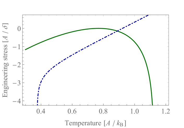
Figure 2: Critical line ($E_{1}=1$, green) of the biaxial solution, and limit of stability of the biaxial solution ($E_{2}=0$; blue, dot-dashed) for a typical paramater value, $\omega=n_{s}\delta^{2}=0.2$. The intersection defines the tricritical point.

In figure 1a, we have drawn the stress-temperature phase diagram for sufficiently small values of the coupling $\omega$. As this coupling parameter increases, the triple and tricritical points approach each other, until they coalesce at $\omega=\omega_{top}$. We can describe this topology change by considering the free energy, given by eq. (32), as a function of $S$, at the tricritical point. In figure 3, we show a plot of $S$ versus the free energy $g$, for $\omega$ between $0.1$ (top curve) and $0.58$ (bottom curve), with the vertical axis shifted so that $g(S_{0})=g_{\text{tri}}=0$. Note that the solution $S=S_{0}$ in eq. (55) becomes metastable at the threshold coupling $\omega=\omega_{top}$. The value of the threshold coupling $\omega_{top}$ comes from the solutions of equations $g(S)=g(S_{0})$ and the equation of state (38), for $S$ ($\neq S_{0}$) and $\omega$, at the tricritical point. Our numerical calculations yield $\omega_{top}\approx 0.59$ and $S_{top}\approx 0.72$. For $\omega>\omega_{top}$, the stress-temperature phase diagram consists of just a first and a second-order transition lines. The first-order transition ends at a simple critical point, and the second-order critical line ends at this first-order border (see (figure 1b)).

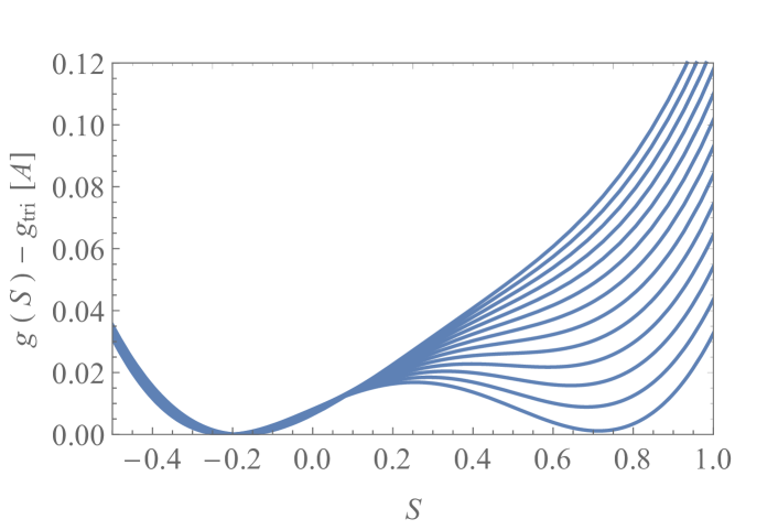
Figure 3: Free energy as a function of the nematic order parameter $S$ at the tricritical point, for $\omega$ between $0.1$ (top curve) and $0.58$ (bottom curve). The vertical axis is shifted so that $g(S_{0})=0$.

The existence of a biaxial phase as well as the asymptotic limit of the second-order transition to a paranematic region can be easily checked in the infinite stress limit. From the equations of state, for $\sigma\delta\rightarrow-\infty$, with $T\neq 0$, we obtain the limiting values

$$S\rightarrow\frac{-\exp\left(-\frac{3}{4}\beta S\right)\cosh\left(\frac{3}{4}\beta\eta\right)}{2\exp\left(-\frac{3}{4}\beta S\right)\cosh\left(\frac{3}{4}\beta\eta\right)}=-\frac{1}{2}$$ (59)

and

$$\eta\rightarrow\frac{3\exp\left(-\frac{3}{4}\beta S\right)\sinh\left(\frac{3}{4}\beta\eta\right)}{2\exp\left(-\frac{3}{4}\beta S\right)\cosh\left(\frac{3}{4}\beta\eta\right)}=\frac{3}{2}\tanh\left(\frac{3}{4}\beta\eta\right).$$ (60)

This second equation already indicates the characteristic up-down symmetry of the biaxial phase in this discrete model system. There is a second order transition at the temperature $T_{c}=9/8=1.125$, which is the previously found asymptotic value of the critical temperature. Using the standard notation for the nematic order parameter, as in equation (27), we have

$$Q =\left(\begin{array}[c]{ccc}-\frac{1}{2}\left(S+\eta\right)&0&0\\ 0&-\frac{1}{2}\left(S-\eta\right)&0\\ 0&0&S\end{array}\right)$$ (64)

$$=\left(\begin{array}[c]{ccc}\frac{1}{4}-\frac{1}{2}\eta&0&0\\ 0&\frac{1}{4}+\frac{1}{2}\eta&0\\ 0&0&-\frac{1}{2}\end{array}\right),$$ (68)

which is a biaxial tensor except at the trivial limits $\eta=0$ (at the second-order transition) and $\eta=\pm 3/2$ (at the ground state).

IV Conclusions

We have analyzed the global phase diagram of a fully-connected version of a Maier-Saupe-Zwanzig lattice model with the inclusion of couplings to an elastic strain field. This is perhaps the simplest model system to be amenable to standard statistical mechanics calculations to investigate elastic effects on a nematic phase transition. We show the presence of uniaxial and biaxial nematic structures, depending on temperature $T$ and on the applied stress $\sigma$. If the applied stress favors uniaxial orientation, we obtain a first-order boundary, along which there is a coexistence of two uniaxial nematic phases, and which ends at a simple critical point. We locate this critical point in terms of the model parameters. This picture is in qualitative agreement with the experimental findings for the behavior of the nematic order parameter of elastomers in a stress field. However, in the presence of a compressive stress, which favors biaxial orientation, we show the existence of a biaxially ordered region. Depending on the strength of the couplings, there is a first-order boundary, but it ends at a tricritical point, beyond which there is a continuous transition to a biaxially ordered structure. We point out the analogy with the behavior of a nematic system in the presence of an applied magnetic (electric) field, depending on the strength of the field and on the sign of the anisotropy. Some of our analytic results, for the critical and tricritical points, for example, may turn out to be a helpful guide to experimental work. In the future, we plan to perform Monte Carlo simulations to make contact with published numerical work Pasini2005 , and to investigate the persistence of these qualitative results in a scenario of short-range interactions.

- (1) M. Warner and M. Terentjev, Liquid Crystal Elastomers, Oxford University Press, Oxford, 2003.
- (2) P. G. de Gennes, C. R. Seances Acad. Sci., Ser. A 281, 101, 1975.
- (3) P. G. de Gennes and J. Prost, The Physics of Liquid Crystals, Clarendon Press, Oxford, 1993.
- (4) P. G. de Gennes and Ko Okumura, Europhys. Lett. 50, 513, 2000.
- (5) S. V. Fridrikh and E. M. Terentjev, Phys. Rev. Lett. 79, 4661, 1997.
- (6) Y.-K. Yu, P. L. Taylor and E. M. Terentjev, Phys. Rev. Lett. 81, 128, 1998.
- (7) J. V. Selinger, H. G. Jeon, and B. R. Ratna, Phys. Rev. Lett. 89, 225701, 2002.
- (8) J. V. Selinger and B. R. Ratna, Phys. Rev. E 70, 041707, 2004.
- (9) S. V. Fridrich and E. M. Terentjev, Phys. Rev. E 60, 1847, 1999.
- (10) L. Petridis and E. M. Terentjev, Phys. Rev. E 74, 051707, 2006.
- (11) Wei Zhu, Michael Shelley, and Peter Palffy-Muhoray, Phys. Rev. E 83, 051703, 2011.
- (12) Danilo B. Liarte, Silvio R. Salinas, and Carlos S. O. Yokoi, Phys. Rev. E 84, 011124, 2011.
- (13) Danilo B. Liarte, Phys. Rev. E 88, 062144, 2013.
- (14) E. do Carmo, A. P. Vieira, S. R. Salinas, Phys. Rev. E 83, 011701, 2011.
- (15) D. B. Liarte and S. R. Salinas, Elementary statistical models for nematic transitions in liquid-crystalline systems, in Perspectives and Challenges in Statistical Physics for the Next Decade, G. M. Viswanathan, E. P. Raposo, M. G. E. da Luz, editors, World Scientific, Singapore, 2014, p. 64.
- (16) A. Petri and S. R. Salinas, Field-induced uniaxial and biaxial nematic phases in the Meier-Saupe-Zwanzig lattice model, unpublished.
- (17) F. Ye, R. Muckhopadhyay, O. Stenull, and T. C. Lubensky, Phys. Rev. Lett. 98, 147801, 2007.
- (18) F. Ye and T. C. Lubensky, J. Phys. Chem. B 113, 3853, 2009.
- (19) J. Küpfer and H. Finkelmann, Makromol. Chem. Rapid Commun. 12, 717, 1991.
- (20) E. S. Nascimento, A. P. Vieira, and S. R. Salinas, Braz. J. Phys. 46, 664 (2016).
- (21) R. M. Hornreich, Phys. Lett. A 109, 232, 1985.
- (22) P. Pasini, G. Skacej, and C. Zannoni, Chem. Phys. Lett 413, 463, 2005.
- (23) P. Palffy-Muhoray and D. A. Dunmur, Mol. Cryst. Liq. Cryst. 97, 337, 1983.
- (24) B. J. Frisken, B. Bergersen, and P. Palffy-Muhoray, Mol. Cryst. Liq. Cryst. 148, 45, 1987.
- (25) E. F. Gramsbergen, L. Longa, and Wim H. de Jeu, Phys. Repts. 135, 195, 1986.