OGLE-2016-BLG-1045: A Test of Cheap Space-Based Microlens Parallaxes

Abstract

Microlensing is a powerful and unique technique to probe isolated objects in the Galaxy. To study the characteristics of these interesting objects based on the microlensing method, measurement of the microlens parallax is required to determine the properties of the lens. Of the various methods to measure microlens parallax, the most routine way is to make simultaneous ground- and space-based observations, i.e., by measuring the space-based microlens parallax. However, space-based campaigns usually require “expensive” resources. Gould & Yee (2012) proposed an idea called the “cheap space-based microlens parallax” that can measure the lens-parallax using only two or three space-based observations of high-magnification events (as seen from Earth). This cost-effective observation strategy to measure microlens parallaxes could be used by space-borne telescopes to build a complete sample for studying isolated objects. This would enable a direct measurement of the mass function including both extremely low-mass objects and high-mass stellar remnants. However, to adopt this idea requires a test to check how it would work in actual situations. Thus, we present the first practical test of this idea using the high-magnification microlensing event OGLE-2016-BLG-1045, for which a subset of Spitzer observations fortuitously duplicate the prescription of Gould & Yee (2012). From the test, we confirm that the measurement of the lens-parallax adopting this idea has sufficient accuracy to determine the physical properties of the isolated lens.

1. Introduction

Isolated objects with various masses such as free-floating planets, brown dwarfs, and black holes are very interesting targets (or potential targets) of study. At the low-mass end, free-floating planets and brown dwarfs may represent the low-mass tail of star formation or the result of bodies ejected during planet formation. Larger-mass objects ($\gtrsim\,$ several Jupiter masses) have been found with direct imaging in star-forming regions (e.g., Bihain et al., 2009; Esplin & Luhman, 2017), and there exist several scenarios to explain their origin and evolution depending on various environmental factors (Whitworth et al., 2007). Microlensing has also probed the free-floating planet population, but with contradictory results. Sumi et al. (2011) argued that Jupiter-mass free-floating planets are about twice as numerous as stars, but Mróz et al. (2017) did not find any evidence for such a population. At the same time, Mróz et al. (2017, 2018) discovered several candidates for less massive (few Earth-mass) free-floating planets. These lower mass objects could be candidates for ejection from forming planetary systems (e.g., Jurić & Tremaine, 2008; Chatterjee et al., 2008; Barclay et al., 2017).

At the high-mass end, there is tension between theoretical predictions of the stellar remnant distribution and the observed population inferred from close binaries. Fryer et al. (2012) predict a smooth distribution of remnant masses ranging from neutron stars to the most massive stellar mass black holes. In contrast, Özel et al. (2012) find a distinct gap between the neutron star and black hole populations in the interval from $\sim 2$ – $5$ $M_{\odot}$. Because the only confirmed black holes are found in binary systems, it is unclear whether this feature (and this conflict between observation and theory) is intrinsic to the mass distribution or somehow specific to stellar remnants in close binaries.

Observations of isolated objects spanning the full mass function are necessary to resolve these issues. Despite the interest of these objects, their discovery and study are challenging because they are generally too faint to find (or they may be entirely dark). Moreover, they have no interaction with other stellar objects. Compared to other methods, the microlensing technique is a powerful and unique tool to probe these isolated objects because the technique can in principle detect any object that approaches or aligns with the line of sight between a background star (source) and observer(s), regardless of the brightness of the objects (lenses).

Unfortunately, microlensing observations do not, by themselves, routinely measure the microlens mass, $M$. Rather, they usually return only the Einstein timescale $t_{\rm E}$, which is a combination of several physical properties of the lens-source system

$$t_{\rm E}\equiv{\theta_{\rm E}\over\mu_{\rm rel}};~{}~{}\theta_{\rm E}\equiv\sqrt{\kappa M\pi_{\rm rel}};~{}~{}\kappa\equiv{4G\over c^{2}\,{\rm au}}\simeq 8.144\,{{\rm mas}\over M_{\odot}}.$$ (1)

Here, ($\pi_{\rm rel},\mbox{\boldmath$\mu$}_{\rm rel}$) are the lens-source relative (parallax, proper motion) and $\mu_{\rm rel}=|\mbox{\boldmath$\mu$}_{\rm rel}|$. Equation (1) implies that to determine the mass $M$ of dark (or at least, unseen) lenses, requires the measurement of both the Einstein radius $\theta_{\rm E}$ and the scalar amplitude $\pi_{\rm E}=|\mbox{\boldmath$\pi$}_{\rm E}|$ of the vector microlens parallax

$$\mbox{\boldmath$\pi$}_{\rm E}\equiv{\pi_{\rm rel}\over\theta_{\rm E}}\,{\mbox{\boldmath$\mu$}_{\rm rel}\over\mu_{\rm rel}};~{}~{}M={\theta_{\rm E}\over\kappa\pi_{\rm E}};~{}~{}\pi_{\rm rel}=\theta_{\rm E}\pi_{\rm E}.$$ (2)

According to Equation (2), the microlens parallax quantifies the lens-source vector displacement as seen from different observers’ positions, relative to the size of the angular Einstein ring radius. The displacements can be caused by the annual motion of Earth, i.e., the annual microlens parallax (hereafter APRX; Gould, 1992), different locations of observatories, such as Earth compared to space-borne telescopes, i.e., the space-based microlens parallax (hereafter SPRX; Refsdal, 1966), or different ground-based sites, i.e., the terrestrial microlens parallax (hereafter TPRX; Gould, 1997).

Each method to measure microlens parallaxes has its limitations. The APRX method (Alcock et al., 1995; Mao, 1999; Smith et al., 2002) requires enough time for the motion of Earth to displace the observer’s position from rectilinear motion enough to measure the parallax. As a result, the APRX can be measured for long timescale events with timescales $t_{\rm E}\gtrsim 30\,$days in favorable cases, but usually $t_{\rm E}\gtrsim 60\,$days. However, these long timescale events are not common. Moreover, from Equations (1) and (2), this method can almost never be applied to low-mass lenses. For the TPRX, the displacement can be provided by a combination of simultaneous observations from ground-based telescopes that are well separated. However, because the size of Earth is only a tiny fraction of the projected Einstein ring on the observer plane ($R_{\oplus}\ll\tilde{r}_{\rm E}\equiv{\rm au}/\pi_{\rm E}$), this measurement can be made for only a few special cases, i.e., extremely magnified lensing events (Gould et al., 2009), for which the strongly divergent magnification pattern is very sensitive to small changes in position. Thus, unfortunately, the chance for TPRX measurements would be extremely rare (Gould & Yee, 2013).

The SPRX method can provide a “routine opportunity” for measuring the microlens parallax as compared to the low chance of measuring lens-parallax with the other methods of the lens-parallax measurements (APRX and TPRX). This is because the displacement of the space-based observatory from the Earth can easily be a significant fraction of the Einstein ring, e.g., Spitzer is $\sim 1.3$ au from Earth compared to a typical value of $\tilde{r}_{\rm E}\sim 10$ au. Refsdal (1966) already proposed this method a half century ago, and Dong et al. (2007) made the first such measurement. Beginning in $2014$, the Spitzer satellite has observed more than $500$ microlensing events with this aim, yielding almost $80$ published microlens parallaxes (Bozza et al., 2016; Calchi Novati et al., 2015a; Chung et al., 2017; Han et al., 2016, 2017; Poleski et al., 2016; Ryu et al., 2018; Shin et al., 2017; Shvartzvald et al., 2015, 2016, 2017; Street et al., 2016; Udalski et al., 2015b; Wang et al., 2017; Yee et al., 2015a; Zhu et al., 2015, 2016, 2017). Even though the SPRX can provide a robust opportunity for measuring microlens parallaxes, there still remains an obstacle to regular adoption of the method because space-based observations usually require “expensive” resources.

Gould & Yee (2012) (hereafter, GY12) proposed to measure “cheap space-based microlens parallaxes (cheap-SPRX)” for high-magnification events (as seen from Earth). They showed that because the lens-source separation (scaled to $\theta_{\rm E}$) $u$ is extremely small near the peak of a high-magnification $A_{\rm max}\gg 1$ event, $u_{0,\oplus}\simeq A^{-1}\rightarrow 0$, the magnitude of the SPRX ($\pi_{\rm E}$) is given by

$$\pi_{\rm E}\simeq{{\rm au}\over D_{\rm sat}}u_{\rm sat}$$ (3)

$$u_{\rm sat}=\sqrt{2[(1-A_{\rm sat}^{-2})^{-1/2}-1]}\sim A_{\rm sat}^{-1}.$$ (4)

Here, $D_{\rm sat}$ is the known projected (on the plane of the sky) separation to the satellite, e.g., $D_{\rm sat}\simeq 1.3$ au for the Spitzer space telescope, and $u_{\rm sat}$ is the position of satellite in the Einstein ring at the exact moment of the peak of the event as seen from Earth. Space-based observations can be used to determine $u_{\rm sat}$ based on $A_{\rm sat}$,

$$A_{\rm sat}={{F_{\rm sat}-F_{\rm base,sat}}\over F_{\rm s,sat}}+1.$$ (5)

The space-based observations provide the $F_{\rm sat}$ (from an observation at the ground-based peak) and $F_{\rm base,sat}$ (from an observation at “baseline”, i.e., well after the event), and ground-based observations can be used to constrain the source $F_{\rm s,sat}$ through color-constraints (Calchi Novati et al., 2015b; Gould et al., 2010a). Hence, we can efficiently determine the magnitude of the microlens parallax for high-magnification events.

The cheap-SPRX is “cheap” in two senses. First, as described in GY12, only two or three space-based observed data points are required to measure the microlens parallax. Second, this technique can be applied to only a small fraction of events (the total number of high-magnification events is inversely proportional to the peak magnification; Gould et al., 2010b). Hence, if a satellite in solar orbit could be equipped with a camera and a means for prompt response for observations, it could carry out such a program at tiny additional cost to its principal mission.

GY12 discussed a potential application of the cheap-SPRX: to study planets through the high-magnification channel. High-magnification events are required for the cheap-SPRX, and they are a very important channel to discover planets because this channel provides almost $100$ per cent detection efficiency if the events contain planetary mass companions to the lens stars (Griest & Safizadeh, 1998). Based on these findings, GY12 argued that the cheap-SPRX could yield an unbiased measurement of the distribution of planets in the Galaxy.

However, since that time, a second major application has emerged: the mass function of isolated objects in the Galaxy (particularly, for low-mass objects). The masses of isolated objects can be measured only if the finite source effect is observed, i.e., if $u_{0}\lesssim\rho_{\ast}$, where $\rho_{\ast}\equiv\theta_{\ast}/\theta_{\rm E}$ and $\theta_{\ast}$ is the angular radius of the source. This generally requires a high-magnification event (since $\rho_{\ast}$ is typically $\mathcal{O}(10^{-3}$ – $10^{-2})$. This is the same condition necessary to measure the cheap-SPRX. Gould (1997) had already noted that high-magnification events could be used to yield isolated masses from a combination of finite source effects and the TPRX. Moreover, two cases were actually observed (Gould et al., 2009; Yee et al., 2009). Gould & Yee (2013) showed the number of these measurements should be $\propto n$, where $n$ is the number density of objects, compared to the underlying microlensing event rate $\propto n\sqrt{M}$, where $M$ is the lens mass. Hence, they are especially useful for measuring the mass function of low-mass objects because these are the most abundant objects in the Galaxy. However, as mentioned above, the chance of measuring such a TPRX is extremely low. Thus, in a practical sense, the study of isolated objects cannot be effectively carried out using the TPRX alone.

Compared to measurements of the TPRX, the SPRX can provide more robust opportunities to make the measurements. Actually, using Spitzer observations, Zhu et al. (2016) and Chung et al. (2017) found that a remarkably high fraction $(3/170)$ of $2015$ Spitzer targets yielded such isolated mass measurements. The principal reason is that Spitzer enables parallax measurements of much larger sources. For TPRX, by contrast, Gould & Yee (2013) showed that the maximum lens distance for which the method could be applied for large sources scales as $D_{\rm L}\propto\theta_{\ast}^{-1}$, implying that the available volume scales as $\theta_{\ast}^{-3}$, thus virtually eliminating large sources for this method. These larger sources have a higher cross-section for crossing the lens, so a better chance of observing finite source effects.

In fact, Spitzer itself is not well matched to the task of systematically measuring cheap-SPRX for high magnification events. Spitzer observations require long lead times ($3-10$ day delay between target selections and start of those observations, see Figure 1 of Udalski et al. 2015b), which raises the possibility of missing very short timescale events, which are most likely to be caused by the lowest mass objects. Moreover, Spitzer can observe the bulge only six weeks out of the eight month bulge season. In addition, the final campaign is currently scheduled to be in $2018$.

As mentioned above, a systematic campaign to measure the cheap-SPRX could be conducted as an “add-on” capability to some future space mission. This would greatly increase the fraction of isolated objects characterized by microlensing. Based on this sample, we can determine the mass function of isolated objects at low cost. However, before pursuing such a course, we should perform a practical test of the cheap-SPRX idea to check the accuracy of the microlens parallax measurement. This test is important because the accuracy that can be achieved is directly related to establishing the feasibility of applying the cheap-SPRX under actual conditions and also for establishing an observational strategy for such a future, space-based microlensing campaign.

Here, we conduct the first practical test for the cheap-SPRX idea using the microlensing event OGLE-2016-BLG-1045 with Spitzer observations. In Section 2.1, we describe the event as a testbed for this practical test. In Section 2.2, we describe our method for testing the idea. Then, we present test results and our findings in Section 2.3. Lastly, we conclude and discuss in Section 3.

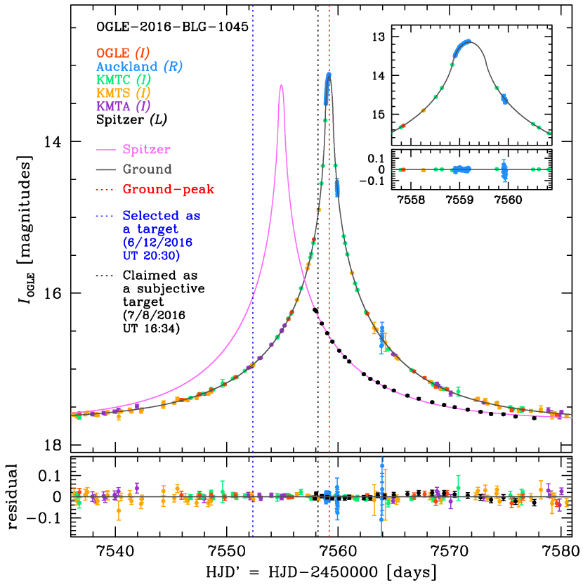
Figure 1.— Light curves of the single-lens event OGLE-2016-BLG-1045 seen from the ground and space. Colored dots represent observed data taken from different telescopes located on the ground and in space (i.e., Spitzer). The dark gray and pink solid lines represent model light curves of the ground and Spitzer, respectively. The red dotted line indicates the peak time ($t_{0}$, see Table 2) of the ground-based light curve. The upper panel shows the observed light curves with their best-fit models. The lower panel shows residuals between the observations and the best-fit model. The inner panel shows the zoom-in of the peak part of ground-based light curve, which has a smooth feature due to the finite source effect. The dotted blue line indicates the time that this event was selected as a Spitzer target. The dotted black line indicates the time that the event was claimed as a subjective target.

2. Test of the Cheap-SPRX Idea

2.1. Testbed: OGLE-2016-BLG-1045 Spitzer event

2.1.1 Ground Observations

The microlensing event OGLE-2016-BLG-1045 occurred on a source that lies at $(\alpha,\delta)_{\rm J2000}=(17^{h}36^{m}51^{s}\\ .19,-34^{\circ}32^{{}^{\prime}}39^{{}^{\prime\prime}}.7)$, which corresponds to the Galactic coordinates $(l,b)=(354.^{\circ}255,-1.^{\circ}386)$. The Optical Gravitational Lensing Experiment (OGLE-IV: Udalski et al., 2015a) found this event and then the Early Warning System (Udalski et al., 1994; Udalski, 2003) of the OGLE-IV survey announced the event on $2016$ June $9$. The observations were made with the $1.3$ m Warsaw telescope in the $I-$band channel of a $1.4$ square-degree camera located at the Las Campanas Observatory in Chile.

The event was highly magnified, implying that a planetary companion to the lens could probably be detected if it exists. Hence, a follow-up observation team called the Microlensing Follow-Up Network ($\mu$FUN: Gould et al., 2006) observed this event to capture any anomalies that might be produced by a planet. Auckland observatory, a $\mu$FUN member located in New Zealand, made the observations with a $0.4$ m telescope using a number $12$ Wratten filter (which is similar to $R-$band). The Auckland observations successfully covered the peak of the event. This peak coverage did not reveal an anomaly in the light curve due to a planetary lens system. However, the good coverage of the peak provided a chance to detect the finite source effect, which enters the determination of the angular Einstein ring radius, i.e., $\rho_{\ast}=\theta_{\ast}/\theta_{\rm E}$. The finite source effect can provide a mass-distance relation, $M/D_{\rm rel}=(c^{2}/4G)~{}\theta_{E}^{2}$, where the $D_{\rm rel}\equiv(D_{\rm L}^{-1}-D_{\rm S}^{-1})^{-1}$ is the relative distance between distances to the lens $(D_{\rm L})$ and the source $(D_{\rm S})$, $M$ is the lens mass, $c$ is the speed of light, and $G$ is the Newton’s constant.

There exist other $\mu$FUN observations in $H-$band taken at the Cerro Tololo International Observatory in Chile with the $1.3$ m SMARTS telescope (CTIO). These CTIO data were not included in the final models because of the similar coverage to the KMTNet data, but were used for the color-magnitude diagram (CMD) analysis of the event (see Appendix).

The Korea Microlensing Telescope Network (KMTNet: Kim et al., 2016) also observed this event. Three identical $1.6$ m telescopes located in the Cerro Tololo International Observatory in Chile (KMTC), the South African Astronomical Observatory in South Africa (KMTS), and the Siding Spring Observatory in Australia (KMTA) observed this event with the $I-$band channel of their $4$ ${\rm deg}^{2}$ cameras. The KMTNet observations provided overall coverage of the light curve.

The observed data sets were reduced by each group using their own pipelines and difference-imaging analysis packages: [(OGLE-IV (DIA): Alard & Lupton, 1998; Wozniak, 2000), ($\mu$FUN and KMTNet (pySIS): Albrow et al., 2009).]

2.1.2 Space Observations

Figure 2.— Light curves showing each test case. The left panel shows the “Actual” case using all actually observed $24$ Spitzer data points. The middle panel shows the “Realistic” case using $3$ selected Spitzer data points considering realistic space-based observations of the cheap-SPRX idea. The right panel shows the “Idealized” case using $2$ artificial data points considering the ideal situation of the cheap-SPRX idea. The gray, black, and red dots indicate ground-based observations, Spitzer observations, and the artificial data, respectively. Black and magenta lines represent the best-fit model light curves of $(-,+)$ solutions of each case.

This event was secretly chosen as a target of the $2016$ Spitzer Microlensing Campaign on $2016$ June $16$ (UT $20$:$30$) based on the possibility that the event could be highly magnified. The event was later claimed as a “subjective” target on $2016$ June $18$ (UT $16$:$34$) once the event was observed to be moderate to high magnification (see Yee et al. 2015b for more details on different types of event selection). The observations began on $2016$ June $18$ (UT $9$:$56$) and ended on July $8$ (UT $2$:$43$). The Spitzer Space Telescope took $24$ total data points over $20$ days with the $3.6$ $\mu$m channel ($L-$band) of the IRAC camera. The Spitzer data were reduced with point response function photometry (Calchi Novati et al., 2015b).

2.1.3 Lightcurves

In Figure 1, we present light curves of the event observed from ground and space. We also present the best-fit model lightcurves and their residuals, which is the $(-,+)$ case presented in Table 2. The ground-based light curve shows a symmetric Paczyński curve (Paczynski, 1986) with a smooth peak feature, which implies that the event was produced by a single lens affected by the finite source effect. The Spitzer observations only partially covered the light curve. However, Han et al. (2017), Shin et al. (2017), and Wang et al. (2017) already showed that it is possible to accurately measure the SPRX even though the space-based observations are fragmentary. Thus, for this event, using the Spitzer observations and the finite source effect, it is possible to measure the microlens parallax and the angular Einstein ring radius, which yield the properties of the isolated lens. We note that there exists a systematic trend in the Spitzer observations. The origin of this trend is unknown. However, several publications that used the Spitzer data with a similar trend (e.g., Poleski et al., 2016; Shin et al., 2017; Shvartzvald et al., 2017; Zhu et al., 2017) concluded that the trend is not likely to affect determinations of their models. In this case, the trend is milder than those in the previous publications.

The Spitzer observations were not taken with the idea of “cheap-SPRX” in mind. In fact, because the peak magnification was relatively unconstrained when the observations were scheduled, many similar events were observed on the chance that one of them would be high-magnification (so, these observations cannot be considered “cheap”). Nevertheless, the resulting observations contain what would be obtained for a “cheap-SPRX” campaign, i.e., the Spitzer observations exist near the peak of the ground-based light curve and also exist near the baseline. Hence, this event can serve as an excellent testbed to perform a practical test of the cheap-SPRX idea.

2.2. Test Method

2.2.1 Three Cases to Test the Cheap-SPRX Measurement

We test the accuracy of the cheap-SPRX method by considering three different Spitzer datasets, which we refer to as the “Actual”, “Realistic”, and “Idealized” cases. These datasets differ in the amount of information they contain (most to least). We first consider the two extremes, which are the “Actual” case defined by the current experiment and the “Idealized” GY12 case. For the “Actual” case, we use all observed Spitzer data ($24$ points). From this case, we can obtain the actual SPRX measurement that can be used as a reference to compare with the measurements derived from the other cases. For the “Idealized” case, considering the ideal situation proposed by GY12, this represents the minimum amount of data necessary for the cheap-SPRX idea to work. For this case, we generate two artificial data points using the Spitzer data and the best-fit model light curve. One is located at the exact ground-based peak (${\rm HJD^{\prime}}=7559.201$) and the other is located at the baseline (${\rm HJD}^{\prime}=7900.000$). For the “Realistic” case, we choose two actual data points near the ground-based peak (${\rm HJD}^{\prime}=7559.172$ and $7559.482$) because it is almost impossible to take an image at the exact peak time in realistic situations. In addition, we use the last point (${\rm HJD}^{\prime}=7577.613$) observed by Spitzer, which is located near the baseline. Based on these selected Spitzer data, we can obtain a measurement of the cheap-SPRX under realistic conditions. In Figure 2, we present light curves of the cases that clearly show the space-based observations used for the test.

2.2.2 Modeling of Lightcurves

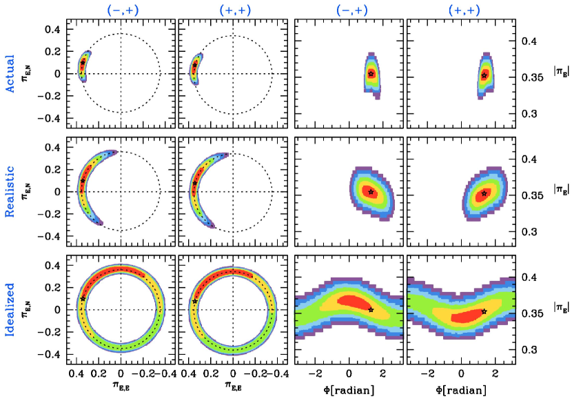
Figure 3.— The SPRX distributions of each case with degenerate solutions. The top, middle, and bottom panels show the SPRX distributions of the actual, realistic, and idealized cases, respectively. The left six panels present the ($\pi_{{\rm E},E}$, $\pi_{{\rm E},N}$) distributions according to the conventional parameterization. The right six panels present the ($\pi_{\rm E}$, $\Phi$) distributions that are the MCMC parameters used to describe the SPRX. The red, yellow, green, light blue, blue, and purple colors represent $\Delta\chi^{2}=1^{2}$, $2^{2}$, $3^{2}$, $4^{2}$, $5^{2}$, and $6^{2}$, respectively. The star symbols indicate the best-fitted SPRX value of the actual case.

Based on the three cases, we conduct modeling to measure the SPRX value of each case. For the modeling, we use six parameters: ($t_{0}$, $u_{0}$, $t_{E}$, $\rho_{\ast}$, $\pi_{\rm E}$, and $\Phi$). Among them, three basic parameters ($t_{0}$, $u_{0}$, and $t_{E}$) describe the light curve produced by a single-lens and a point-source. These basic parameters are closely related to each other: $t_{0}$ is the time at the peak of the light curve; $u_{0}$ is the impact parameter, i.e., the separation between the center of the Einstein ring and the position of the source at time $t_{0}$; $t_{\rm E}$ is the crossing-time of the Einstein ring. Another parameter $\rho_{\ast}$ is the angular source radius ($\theta_{\ast}$) normalized by the angular Einstein ring radius ($\theta_{\rm E}$), $\rho_{\ast}\equiv\theta_{\ast}/\theta_{\rm E}$, which describes the finite source effect. The last two parameters ($\pi_{\rm E}$ and $\Phi$) describe the SPRX, which differs from the conventional way of describing the microlens parallax vector $\pi$ (normally consisting of North ($\pi_{{\rm E},N}$) and East ($\pi_{{\rm E},E}$) components). In our parameterization (see also Bennett et al. 2008),

$$\mbox{\boldmath$\pi$}_{\rm E}=(\pi_{{\rm E},N},\pi_{{\rm E},E})\rightarrow(\pi_{\rm E}\cos\Phi,\pi_{\rm E}\sin\Phi).$$ (6)

The $\Phi$ angle is allowed to vary over the full possible range $[-\pi,+\pi]$. In addition, there are flux parameters ($F_{S}$ and $F_{B}$) for each data set that describe the fluxes of the source and blend, respectively, which are fit linearly for each model. We note that the model flux for each dataset, $i$, is derived from $F_{{\rm obs},i}(t)={\rm A}(t)F_{S,i}+F_{B,i}$, where the ${\rm A}(t)$ is the model magnification as a function of time. Using these parameters, we search for the best-fit model with the minimum $\chi^{2}$ between the observed and modeled light curves using a Markov Chain Monte Carlo (MCMC) $\chi^{2}$ minimization (the details of our MCMC sampling method are described in Dunkley et al., 2005). To find the global minimum of the model parameters, especially the SPRX parameter ($\pi_{\rm E}$), we initially conducted a grid search over $\pi_{\rm E}$ and $\Phi$ using the $200$x$200$ grid points. The grid search results are same as those of the MCMC simulations.

Table 1Limb-darkening coefficients and error re-scaling factors

Observations	$\Gamma_{\lambda}$	$k$
OGLE (I)	0.5103	0.913
Auckland (R)†	0.6583	2.370
KMTC (I)	0.5103	1.116
KMTS (I)	0.5103	1.501
KMTA (I)	0.5103	1.446

Note. — ^†We use a modified LD coefficient for Auckland observations, $\Gamma_{R}=(\Gamma_{R}+\Gamma_{V})/2=(0.61118+0.7048)/2=0.6583$ because the Auckland observatory used a $12$ Wratten filter having a flat transmission between $540-700$ nm. Thus, the filter is similar to the mean value of $R-$ and $V-$bands. Note that we did not use a $\Gamma_{L}$ because it plays no role for the Spitzer observations.

Table 2The best-fit model with degenerate solutions of each case

Case	Actual		Realistic		Idealized
parameter	$(-,+)$	$(+,+)$	$(-,+)$	$(+,+)$	$(-,+)$	$(+,+)$
$\chi^{2}_{\rm total}/N_{\rm data}$	1368.70 / 1372	1368.99 / 1372	1344.89 / 1351	1345.04 / 1351	1343.83 / 1350	1343.95 / 1350
$\chi^{2}_{\rm Ground}/N_{\rm data}$	1345.01 / 1348	1345.09 / 1348	1344.77 / 1348	1344.77 / 1348	1343.83 / 1348	1343.95 / 1348
$\chi^{2}_{\it Spitzer}/N_{\rm data}$	23.69 / 24	23.90 / 24	0.12 / 3	0.27 / 3	0.00 / 2	0.00 / 2
$\chi^{2}_{\rm penalty}$	0.017	0.075	0.000	0.010	0.003	0.014
$(I-L)$ [3.80]	3.797	3.794	3.800	3.802	3.799	3.803
$t_{0}$ (HJD’)	7559.201$\pm$0.001	7559.201$\pm$0.001	7559.201$\pm$0.001	7559.201$\pm$0.001	7559.202$\pm$0.001	7559.202$\pm$0.001
$u_{0}$ ($10^{-2}$)	-1.308${}_{-0.042}^{+0.033}$	1.314${}_{-0.044}^{+0.036}$	-1.318${}_{-0.037}^{+0.041}$	1.318${}_{-0.044}^{+0.033}$	-1.312${}_{-0.044}^{+0.033}$	1.309${}_{-0.033}^{+0.044}$
$t_{\rm E}$ (days)	11.981${}_{-0.098}^{+0.064}$	11.963${}_{-0.084}^{+0.088}$	11.950${}_{-0.083}^{+0.084}$	11.947${}_{-0.083}^{+0.088}$	11.956${}_{-0.094}^{+0.073}$	11.952${}_{-0.088}^{+0.076}$
$\rho_{\ast}$ ($10^{-2}$)	3.186${}_{-0.026}^{+0.033}$	3.190${}_{-0.030}^{+0.030}$	3.195${}_{-0.030}^{+0.027}$	3.195${}_{-0.033}^{+0.028}$	3.194${}_{-0.029}^{+0.030}$	3.193${}_{-0.028}^{+0.031}$
$\pi_{\rm E}$	0.355${}_{-0.006}^{+0.004}$	0.352${}_{-0.005}^{+0.006}$	0.355${}_{-0.008}^{+0.005}$	0.350${}_{-0.006}^{+0.008}$	0.365${}_{-0.015}^{+0.004}$	0.346${}_{-0.004}^{+0.014}$
$\Phi$ (radian)	1.291${}_{-0.062}^{+0.165}$	1.353${}_{-0.066}^{+0.167}$	1.210${}_{-0.284}^{+0.381}$	1.178${}_{-0.177}^{+0.458}$	0.341${}_{-1.185}^{+0.955}$	0.407${}_{-1.188}^{+1.141}$
$\pi_{{\rm E},{\it E}}$	0.341${}_{-0.012}^{+0.012}$	0.344${}_{-0.011}^{+0.013}$	0.332	0.323	0.122	0.137
$\pi_{{\rm E},{\it N}}$	0.098${}_{-0.059}^{+0.027}$	0.076${}_{-0.058}^{+0.028}$	0.125	0.134	0.344	0.317
$F_{\rm S,OGLE}$	1.370${}_{-0.010}^{+0.014}$	1.373${}_{-0.013}^{+0.012}$	1.375${}_{-0.012}^{+0.012}$	1.375${}_{-0.013}^{+0.011}$	1.374${}_{-0.011}^{+0.014}$	1.374${}_{-0.012}^{+0.013}$
$F_{\rm B,OGLE}$	-0.032${}_{-0.014}^{+0.010}$	-0.034${}_{-0.012}^{+0.012}$	-0.036${}_{-0.012}^{+0.011}$	-0.037${}_{-0.012}^{+0.012}$	-0.035${}_{-0.014}^{+0.010}$	-0.036${}_{-0.013}^{+0.011}$
$F_{\rm S,{\it Spitzer}}$	45.257${}_{-0.932}^{+0.919}$	45.212${}_{-0.870}^{+1.004}$	45.518${}_{-1.061}^{+0.953}$	45.622${}_{-1.199}^{+0.902}$	45.439${}_{-0.909}^{+1.124}$	45.618${}_{-1.127}^{+0.973}$
$F_{\rm B,{\it Spitzer}}$	-6.528${}_{-0.993}^{+0.941}$	-6.430${}_{-1.178}^{+0.819}$	-8.032${}_{-1.094}^{+0.963}$	-8.179${}_{-1.046}^{+1.174}$	-6.674${}_{-1.190}^{+0.844}$	-6.854${}_{-1.039}^{+1.062}$

Note. — ${\rm HJD^{\prime}=HJD-2450000.0}$. The $N_{\rm data}$ after each $\chi^{2}$ value indicates the number of data points that are used for the modeling. We note that the $\pi_{{\rm E},E}$ and $\pi_{{\rm E},E}$ are not modeling parameters. These are calculated from the modeling parameters, $\pi_{\rm E}$ and $\Phi$ (see Equation (6)). We do not present the errors of $\pi_{{\rm E},N}$ and $\pi_{{\rm E},E}$ for Realistic and Idealized cases because these errors are meaningless: only the error in $\pi_{\rm E}$ has meaning.

During the modeling process, we consider the limb-darkening (LD) of the source star. We adopt LD coefficients for observed passbands from Claret (2000) based on the spectral source type determined by the CMD analysis (described in the Appendix). In addition, we re-scale the errors of observations to enforce $\chi^{2}/{\rm dof}\simeq 1$ using the equation $e_{\rm new}=k(e_{\rm old})$ where $k$, $e_{\rm new}$, and, $e_{\rm old}$ are the error re-scaling factor, re-scaled errors, and original errors, respectively. The error re-scaling process has been done based on the best-fit model, i.e., the $(-,+)$ case. We note that, in the case of the OGLE-IV data, the observational errors are calibrated using a correction procedure that is described in Skowron et al. (2016), before applying the error re-scaling process based on the best-fit model. In Table 1, we present these LD coefficients and error re-scaling factors for modeling.

We also incorporate the color-constraint, $(I-L)=3.800\pm 0.020$, which provides an independent constraint on the model. The constraint is determined using $I-$band ground observations (OGLE-IV) and $L-$band space observations (Spitzer) based on the CMD analysis. To incorporate the ($I-L$) color-constraint, we introduce $\chi^{2}_{\rm penalty}$ described in Section 3.2 of Shin et al. (2017). The $\chi^{2}_{\rm penalty}$ increases the $\chi^{2}$ when the fitted ($I-L$) color of the model is different from the constraint. In particular, the $\chi^{2}_{\rm penalty}$ increases strongly when the difference between the fitted color and the constraint is larger than $2\sigma$.

In Table 2, we present the best-fit parameters for each case (Actual, Realistic, Idealized). For each case, we find that there exist two degenerate solutions due to the “four-fold degeneracy” (Refsdal, 1966; Gould, 1994). In principle, the four-fold degeneracy has four solutions, $(+,+)$, $(+,-)$, $(-,+)$, and $(-,-)$ (denoted according to the convention described in Zhu et al. 2015), which are caused by different pairs of source trajectories (seen from ground and space) going through a similar lensing magnification pattern. This degeneracy can be divided into two categories by its origin (GY12 and references therein). The first (denoted by the first $\pm$ sign in this paper) is related to the relative positions of the Earth and satellite, whether they lie on the same or opposite sides of the lens. The other (denoted by the second $\pm$ sign in this paper) is related to the different possible source trajectories as seen from Earth, i.e., whether they pass on the left or right sides of the lens. The former degeneracy can affect the magnitude ($\pi_{\rm E}$) of the $\mbox{\boldmath$\pi$}_{\rm E}$, while the latter degeneracy can only affect the direction of the $\mbox{\boldmath$\pi$}_{\rm E}$, which is less interesting in this test of the cheap-SPRX idea. The four-fold degeneracy can sometimes be resolved (e.g., Chung et al., 2017; Han et al., 2016, 2017; Shin et al., 2017; Udalski et al., 2015b; Yee et al., 2015a). For this event, we find that there exist only two solutions, $(-,+)$ and $(+,+)$, based on the grid search process. The other two solutions, $(-,-)$ and $(+,-)$, are merged with the $(-,+)$ and $(+,+)$ solutions, respectively. The reason that the four solutions are merged into only two solutions for this event is that $u_{0,Spitzer}\sim 0$. For model parameters of each solution, uncertainties are determined based on the $68\%$ confidence intervals of the MCMC chains.

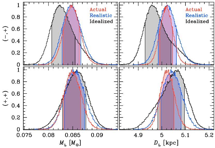
Figure 4.— Distributions of lens properties determined from the MCMC chains. The left-side upper and lower panels show the lens mass distributions of $(-,+)$ and $(+,+)$ solutions, respectively. The right-side upper and lower panels show the distributions of the distance to the lens of $(-,+)$ and $(+,+)$ solutions, respectively. The red, blue, and black colors indicate the actual, realistic, and idealized case, respectively. The colored shade shows the $1\,\sigma$ uncertainty ($68\%$ area of the distributions) of each case. Each distribution is normalized so the peak of the histogram is set to unity.

2.3. Test Results

2.3.1 Validation of the Accuracy of the Cheap-SPRX Measurement

In Figure 3, we present the SPRX distributions of each case. The distributions are constructed from the MCMC chains. These distributions clearly show the consistency of the SPRX measurements. We present two types of distributions. One type of distribution is presented according to the conventional parameters, $(\pi_{{\rm E},E},\pi_{{\rm E},N})$, which are calculated from the MCMC parameters as $\pi_{{\rm E},E}=\pi_{\rm E}\sin{\Phi}$ and $\pi_{{\rm E},N}=\pi_{\rm E}\cos{\Phi}$. The other is the ($\pi_{\rm E}$, $\Phi$) distribution, which can be used to directly check the accuracy of the magnitude of the SPRX measurement.

From the modeling of the actual case, we obtain the SPRX measurements for the $(-,+)$ and $(+,+)$ cases: $\pi_{\rm E}=0.355^{+0.004}_{-0.006}$ and $0.352^{+0.006}_{-0.005}$, respectively. We find that the magnitudes of the SPRX values between the $(-,+)$ and $(+,+)$ solutions of the actual case are consistent to well within $1\sigma$. Based on the actual SPRX measurements, we can compare the other test cases of the cheap-SPRX idea to check the accuracy of the cheap-SPRX measurements. For the realistic case, we find that the SPRX measurements of both degenerate solutions, $0.355^{+0.005}_{-0.008}$ and $0.350^{+0.008}_{-0.006}$, are consistent with those of the actual case to within $1\sigma$. For the idealized case, the measurements, $0.365^{+0.004}_{-0.015}$ and $0.346^{+0.014}_{-0.004}$, are consistent to within $\lesssim 1\sigma$ using the idealized-case errors.

Based on the SPRX measurements, we can determine the properties of this isolated lens by combining it with the angular Einstein ring radius ($\theta_{\rm E}=\theta_{\ast}/\rho_{\ast}$), where $\theta_{\ast}$ is the angular source radius determined from the CMD analysis (described in the Appendix) and $\rho_{\ast}$ is determined from the finite source effect. We determine the angular Einstein ring radius as

$$\theta_{\rm E}=0.244\pm 0.015~{}{\rm mas}.$$ (7)

In Figure 4, we present distributions of physical properties of the lens for each case. the lens mass ($M_{\rm L}$) and the lens distance ($D_{\rm L}$) are determined from MCMC parameters as

$$M_{\rm L}={(\theta_{\ast}/\kappa)\over{\rho_{\ast}\pi_{\rm E}}},~{}~{}\kappa=8.144~{}{\rm mas}\,M_{\odot}^{-1},$$ (8)

$$D_{\rm L}={{\rm au}\over{(\pi_{\rm E}/\rho_{\ast})\,\theta_{\ast}+\pi_{S}}},~{}~{}\pi_{S}={{\rm au}\over D_{S}},$$ (9)

where $D_{S}$ is the distance to the source estimated from Nataf et al. (2013). For this event, the estimated $D_{S}$ is $\sim 8.87\,$ kpc. We find that both properties are consistent to within $1\sigma$ across all cases. In fact, the uncertainty in the properties is dominated by the uncertainty of the $\theta_{\ast}$ determination. Quantitatively, the uncertainty of the SPRX measurement is $<3\%$ compared to the $\geq 6\%$ uncertainty in $\theta_{\ast}$. Thus, we find that the accuracy of the SPRX measurement based on the cheap-SPRX idea is sufficient to accurately determine the properties of the isolated object. The isolated lens of this event is a low-mass stellar object with $M_{\rm L}\sim 0.08\pm 0.01\,M_{\odot}$, which is located at $\sim 5.02\pm 0.14\,$ kpc from us .

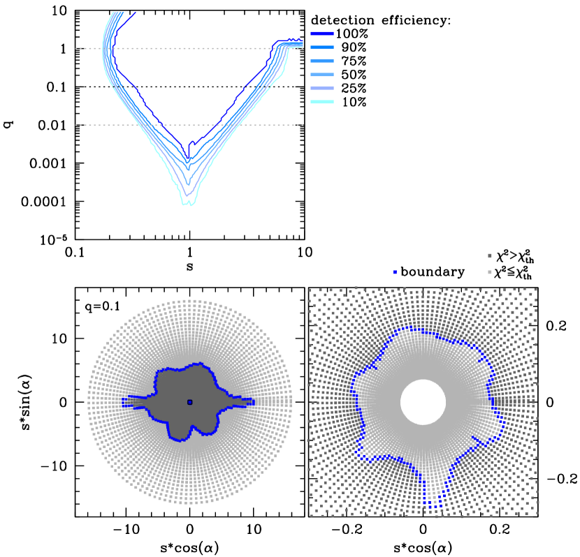
Figure 5.— Example of diagrams at the mass ratio ($q=0.1$) and their boundaries. The upper panel shows the detection efficiency diagram built using $\chi^{2}_{\rm th}=15.0$. The lower panels show diagrams of the two regimes of binary lensing for the case of $q=0.1$. The left panel shows the wide ($s>1$) binary regime and the right panel shows the close ($s<1$) binary regime. The grey and dark grey dots represent two categories of binary-lensing cases whose boundary is given by $\chi^{2}_{\rm th}$. The grey dots indicate $\chi^{2}\leq 15.0$, while the dark grey dots indicate $\chi^{2}>15.0$. The blue dots indicate the boundary points between the two categories.

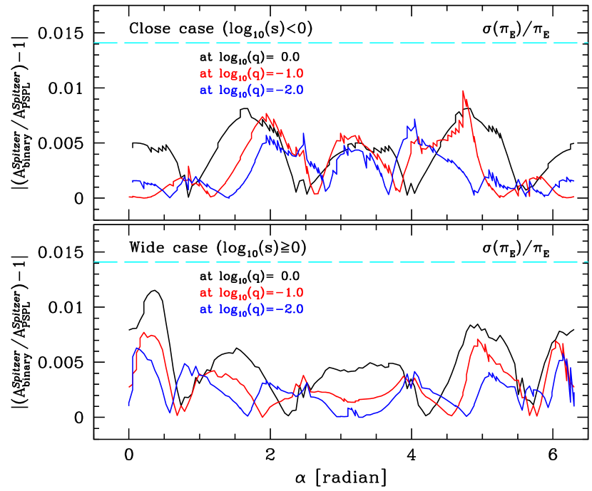
Figure 6.— The criterion values of the test from the boundary cases. The upper and lower panels show the criterion values for the close and wide binary cases, respectively. The black, red, and blue colors represent the magnification deviations of boundaries at $q=0.01,\,0.1,$ and $1.0$, respectively. The cyan dashed line represents the relative error of the measured SPRX value.

2.3.2 Validation of Effects on the Cheap-SPRX Measurement by Binary-lensing Cases

The cheap-SPRX idea assumes that an observed lightcurve seen from space, e.g., the Spitzer observations, resembles a single-lensing lightcurve. However, if the lens is a binary and there are only two observations from the spacecraft, it will not be possible to determine from the space-based observations alone whether these are affected by the binary or whether the single-lens assumption is sufficient. Indeed, if the binary is not detected in the ground-based data, an anomaly in the space-based data due to a binary would go undetected. Then, the magnification computation to measure the cheap-SPRX may be inaccurately determined due to the effect of the binary-lensing perturbation on the lightcurve. As a result, a violation of the single-lensing assumption can in principle yield an incorrect measurement of the cheap-SPRX when a second mass exists.

However, high-magnification events (this is a basic assumption for applying the cheap-SPRX idea) are very sensitive to binary lenses. This implies that, for a high-magnification event, we can rule out a very broad class binary-lens configurations because these would produce clear anomalies on the ground-based lightcurve. We perform a quantitative test to check the effect on the cheap-SPRX measurement caused by binary-lensing. The test is performed using the following procedures.

First, we separately conduct a binary-lens modeling with ground-based observations only. The best-fitting of this modeling yields a $\chi^{2}$ threshold to exclude binary-lensing cases, which have noticeable anomalies. The best-fit model has $\Delta\chi^{2}=(\chi^{2}_{\rm single}-\chi^{2}_{\rm binary})=13.9$. Thus, we set the $\chi^{2}$ threshold $\chi^{2}_{\rm th}=15.0$. This is the criterion for dividing simulated binary-lensing cases into two categories: $\chi^{2}>\chi^{2}_{\rm th}$ are the cases with anomalies that are detectable in the ground-based lightcurve, and $\chi^{2}<\chi^{2}_{\rm th}$ are the cases having non-detectable anomalies.

Second, we simulate binary-lensing cases with only ground-based observations using the Rhie method (Bennett & Rhie, 1996; Rhie et al., 2000). In this procedure, the binary-lensing cases are simulated using a grid of the projected separation ($s$), mass ratio ($q$), and angle ($\alpha$) of the source trajectory with respect to the binary-axis: $\log{s}=[-1.2,\,1.2]$, $\log{q}=[-5.0,\,1.0]$, and $\alpha=[0,\,2\pi]$. Each range of the grid is divided into $120$ grid points (i.e., total $120^{3}$ binary-lensing cases are simulated). We adopt the other parameters, $t_{0}$, $u_{0}$, $t_{\rm E}$, and $\rho_{\ast}$, from the actual $(-,+)$ solution to produce an artificial dataset of the binary-lensing case. For each binary-lensing case with the artificial ground-based dataset, we calculate a $\chi^{2}$ value by fitting with a finite-source single-lensing model.

Third, we can build two types of diagrams (Figure 5) using the simulated binary-lensing cases and the $\chi^{2}$ threshold: one is the diagram showing the detection efficiency of this event, and the other is the diagram showing two categories of the binary-lensing cases at a specified mass ratio. From this diagram, we can extract a “boundary” with $\Delta\chi^{2}=15$, which represents a kinds of extreme binary-lensing cases having non-detectable anomalies that may possibly affect the cheap-SPRX measurement. In Figure 5, we present an example of such diagrams at the $q=0.1$ and their boundaries.

Fourth, at these boundary cases, we can check the effect on the cheap-SPRX measurement caused by the hidden anomalies of the binary-lensing cases. To quantitatively check the effect, we set a criterion as

$$\left|\frac{A_{\rm binary}^{Spitzer}}{A_{\rm PSPL}^{Spitzer}}-1\right|_{\rm peak,\oplus}<\frac{\sigma(\pi_{\rm E})}{\pi_{\rm E}}$$ (10)

where the $A_{\rm binary}^{Spitzer}$ and $A_{\rm PSPL}^{Spitzer}$ are magnifications of the Spitzer lightcurve at the ground-peak time (HJD’$\sim 7559.20$) computed using binary-lens and single-lens models, respectively. The $\pi_{\rm E}$ and $\sigma(\pi_{\rm E})$ are the cheap-SPRX measurement and its uncertainty adopted from the actual $(-,+)$ case. This criterion shows how much an undetected anomaly due to binary-lensing could affect the magnification of the Spitzer lightcurve. If the criterion in Equation (10) is met, the inaccuracy in the magnification is less significant than uncertainties from other sources. Using this criterion, we check three cases of boundaries at $q=0.01,\,0.1,$ and $1.0$.

In Figure 6, we present the quantitative results of this test. We find that, for all cases along the boundary, the deviations between magnifications of the Spitzer lightcurve at the ground-peak are much smaller than the relative error of the SPRX that is actually measured. This implies that the binaries that do not give to detectable signals in the ground-based data also do not significantly affect the SPRX measurement. Hence, in this case, even if there exists an undetected binary-lens anomaly, we can still obtain an accurate SPRX measurement using the cheap-SPRX idea.

3. Conclusion and Discussion

Based on the event OGLE-2016-BLG-1045, we tested the cheap-SPRX idea to check the accuracy of the microlens parallax measurement by comparing it to the true measurement. In addition, based on the parallax measurement of each case, we checked whether the physical properties of this isolated lens are consistent or not. We found that the magnitudes of the actual SPRX measurement and the realistic, cheap-SPRX measurement are consistent to within $1\sigma$. We also found that the lens mass determined for all cases is consistent $\sim 0.08$ $M_{\odot}$, which is the upper-mass limit for brown dwarfs. In addition, the lens distances derived for all cases are also consistent to within $1\sigma$. Moreover, we conducted a test to see how a binary lens that is not detectable in ground-based observations might affect the cheap-SPRX measurement. We found that this effect is not significant in this case. Hence, we conclude that the cheap-SPRX measurement has sufficient accuracy to adopt this idea in real situations. Thus, using only two or three space-based observations, we can determine the physical properties of the lens for high-magnification events. This fact implies that by adopting the cheap-SPRX idea, we have a robust method of measuring microlens parallaxes (i.e., SPRX), which can reveal the nature of the lens with a cost-effective space-based campaign.

A space-based microlensing campaign, perhaps added on to another mission, adopting this cost-effective idea can provide a measurement of the magnitude of the microlens parallax for most high-magnification events. This complete sample can be used to study isolated objects, especially low-mass objects, in the Galaxy and derive a mass function based on them.

Appendix A The Color-Magnitude diagram (CMD) Analysis

From this CMD analysis, we can determine the angular source radius, the spectral type of the source star, and the model-independent color constraint. The CMD analysis is usually conducted by combining the $(V-I,I)$ CMD and the standard method (Yoo et al., 2004). However, for this event, the source is severely extincted with $A_{I}\sim 3.5$ in $I-$band. As a result, the standard method cannot be applied using the $(V-I,I)$ CMD. Hence, we construct a new $(I-H,I)$ CMD based on the OGLE-IV survey and the VISTA Variables and Via Lactea Survey (VVV: Minniti et al., 2010) using cross-matching of field stars, which are located within $60^{\prime\prime}$ from the source star.

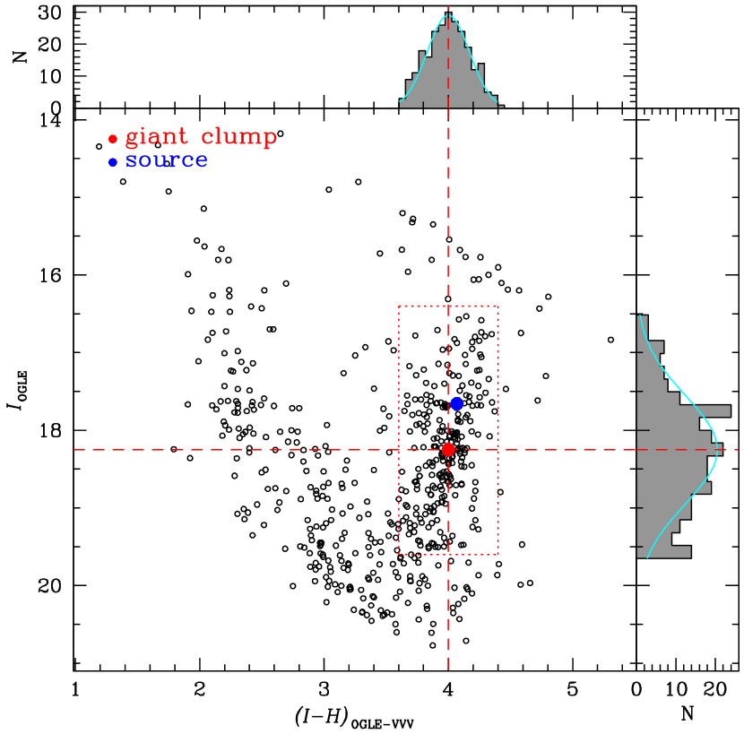
Figure 7.— The $(I-H,I)$ CMD of the OGLE-2016-BLG-1045 event. The CMD is constructed by cross-matching OGLE-IV and VVV observations. The red and blue dots indicate the red giant clump centroid and the source, respectively. We present color and magnitude distributions of field stars within a selected region, which is a box marked in red dotted lines, along with the abscissa and ordinate, respectively. The cyan line indicates the Gaussian fitting of the distributions. The location of the red giant clump centroid is determined from these distributions.

In Figure 7, we present the $(I-H,I)$ CMD. We conduct the CMD analysis using the standard method. First, we determine the location of the red giant clump centroid on the CMD as $(I-H,I)_{\rm C}=(4.00\pm 0.03,18.25\pm 0.05)$. Second, the location of the source on the CMD is determined based on source fluxes in $I$ band and $H$ band from the best-fit model additionally including CTIO $H-$band data. The magnitudes are found to be $I_{S,{\rm OGLE}}=17.658\pm 0.004$ and $H_{S,{\rm CTIO}}=17.648\pm 0.003$. The CTIO $H-$magnitude scale is converted to the VVV $H-$magnitude scale using the relation $(H_{\rm CTIO}-H_{\rm VVV})_{\rm S}=4.059\pm 0.011$, which comes from comparison stars. Thus, the location of the source on the CMD is determined to be $(I-H,I)_{\rm S}=(4.068\pm 0.012,17.658\pm 0.004)$.

We adopt the de-reddened color (Bensby et al., 2013) and intrinsic magnitude (Nataf et al., 2013) of the giant clump as a reference. The adopted values are $(V-I,I)_{0,{\rm C}}=(1.06\pm 0.01,14.62\pm 0.04)$. Based on this reference, we can obtain the de-reddened color and magnitude of the source under the assumption that the clump and source experience the same extinction. In addition, the $(I-H)$ color is converted to the $(V-I)$ color using the color-color relation in Bessell & Brett (1988). For the source of this event, the relation is $\Delta(I-H)=1.00\times\Delta(V-I)$. Thus, the de-reddened color and magnitude of the source are $(V-I)_{0,{\rm S}}=(V-I)_{0,{\rm C}}-[(I-H)_{\rm C}-(I-H)_{\rm S}]$ and $I_{0,{\rm S}}=I_{0,{\rm C}}-[I_{\rm C}-I_{\rm S}]$, respectively. Lastly, we obtain the de-reddened color and magnitude of the source: $(V-I,I)_{0,{\rm S}}=(1.128\pm 0.034,14.028\pm 0.064)$.

From the color of the source, we determine the angular source radius using the color/surface-brightness relations in Kervella et al. (2004). To employ the relation, we convert the $(V-I)_{0,{\rm S}}$ to $(V-I)_{0,{\rm S}}$ by using the Bessell & Brett (1988) relation. The determined angular source radius is

$$\theta_{\ast}=7.80\pm 0.47~{}~{}{\rm{\mu}as}.$$ (A1)

Moreover, based on the intrinsic source color, we estimate the source star to be an early K-type giant. We adopt LD coefficients from Claret (2000) assuming typical properties of an early K-type giant: effective temperature $T_{\rm eff}\simeq 4750$ K, surface gravity $\log{g}\simeq 2.0$, microturbulent velocity $V_{t}\simeq 2.0$ ${\rm km\,s^{-1}}$, and metallicity $\log{[M/H]}\simeq 0.0$. The adopted LD coefficients are presented in Table 1.

Based on the information of the source, we determine the $(I-L)$ color constraint using the color-color regression method based on the $IHL$ color-color diagram. This process is described in Calchi Novati et al. (2015b) and Shin et al. (2017). The determined $(I-L)$ color constraint is

$$(I-L)=3.800\pm 0.020.$$ (A2)

We incorporate this model-independent constraint in the modeling process by introducing an additional $\chi^{2}_{\rm penalty}$, which increases as $\Delta(I-L)$ increases between the color calculated from the model and the constraint.

References

- Alard & Lupton (1998) Alard, C. & Lupton, Robert H. 1998, ApJ, 503, 325
- Albrow et al. (2009) Albrow, M. D., Horne, K., Bramich, D. M., et al. 2009, MNRAS, 397, 2099
- Alcock et al. (1995) Alcock, C., Allsman, R. A., Alves, D., et al. 1995, ApJ, 454, L125
- Barclay et al. (2017) Barclay, T., Quintana, E. V., Raymond, S. N., et al. 2017, ApJ, 841, 86
- Bennett et al. (2008) Bennett, D.P., Bond, I.A., Udalski, A., et al. 2008, ApJ, 684, 663
- Bennett & Rhie (1996) Bennett, D. P., & Rhie, S. H. 1996, ApJ, 472, 660
- Bensby et al. (2013) Bensby, T., Yee, J. C., Feltzing, S., et al. 2013, A&A, 549, 147
- Bessell & Brett (1988) Bessell, M. S., & Brett, J. M. 1988, PASP, 100, 1134
- Bihain et al. (2009) Bihain, G., Rebolo, R., Zapatero Osorio, M. R., et al. 2009, A&A, 506, 1169
- Bozza et al. (2016) Bozza, V., Shvartzvald, Y., Udalski, A., et al. 2016, ApJ, 820, 79
- Calchi Novati et al. (2015a) Calchi Novati, S., Gould, A., Udalski, A., et al. 2015a, ApJ, 804, 20
- Calchi Novati et al. (2015b) Calchi Novati, S., Gould, A., Yee, J. C., et al. 2015b, ApJ, 814, 92
- Chatterjee et al. (2008) Chatterjee, S., Ford, E. B., Matsumura, S., et al. 2008, ApJ, 686, 580
- Chung et al. (2017) Chung, S.-J., Zhu, W., Udalski, A., et al. 2017, ApJ, 838, 154
- Claret (2000) Claret, A. 2000, A&A, 363, 1081
- Dong et al. (2007) Dong, S., Udalski, A., Gould, A., et al. 2007, ApJ, 664, 862
- Dunkley et al. (2005) Dunkley, J., Bucher, M., Ferreira, P. G., et al. 2005, MNRAS, 356, 925
- Esplin & Luhman (2017) Esplin, T. L., & Luhman, K. L. 2017, AJ, 154, 134
- Fryer et al. (2012) Fryer, C. L., Belczynski, K., Wiktorowicz, G., et al. 2012, ApJ, 749, 91
- Gould (1992) Gould, A. 1992, ApJ, 392, 442
- Gould (1994) Gould, A. 1994, ApJ, 421, L75
- Gould (1997) Gould, A. 1997, ApJ, 480, 188
- Gould et al. (2010a) Gould, A., Dong, S., Bennett, D. P., et al. 2010a, ApJ, 710, 1800
- Gould et al. (2010b) Gould, A., Dong, S., Gaudi, B. S., et al. 2010b, ApJ, 720, 1073
- Gould et al. (2006) Gould, A., Udalski, A., An, D., et al. 2006, ApJ, 644, L37
- Gould et al. (2009) Gould, A., Udalski, A., Monard, B., et al. 2009, ApJ, 698, L147
- Gould & Yee (2012) Gould, A., & Yee, J. C. 2012, ApJ, 755, L17
- Gould & Yee (2013) Gould, A., & Yee, J. C. 2013, ApJ, 764, 107
- Griest & Safizadeh (1998) Griest, K., & Safizadeh, N. 1998, ApJ, 500, 37
- Han et al. (2016) Han, C., Udalski, A., Gould, A., et al. 2016, ApJ, 828, 53
- Han et al. (2017) Han, C., Udalski, A., Gould, A., et al. 2017, ApJ, 834, 82
- Jurić & Tremaine (2008) Jurić, M., & Tremaine, S. 2008, ApJ, 686, 603
- Kervella et al. (2004) Kervella, P., Bersier, D., Mourard, D., et al. 2004, A&A, 428, 587
- Kim et al. (2016) Kim, S.-L., Lee, C.-U., Park, B.-G., et al. 2016, JKAS, 49, 37
- Mao (1999) Mao, S. 1999, A&A, 350, L19
- Minniti et al. (2010) Minniti, D., Lucas, P. W., Emerson, J. P., et al. 2010, NewA, 15, 433
- Mróz et al. (2017) Mróz, P., Udalski, A., Skowron, J., et al. 2017, Nature, 548, 183
- Mróz et al. (2018) Mróz, P., Ryu, Y.-H., Skowron, J., et al. 2018, AJ, 155, 121
- Nataf et al. (2013) Nataf, D. M., Gould, A., Fouqué, P., et al. 2013, ApJ, 769, 88
- Özel et al. (2012) Özel, F., Psaltis, D., Narayan, R., et al. 2012, ApJ, 757, 55
- Paczynski (1986) Paczyński, B. 1986, ApJ, 304, 1
- Poleski et al. (2016) Poleski, R., Zhu, W., Christie, G. W., et al. 2016, ApJ, 823, 63
- Refsdal (1966) Refsdal, S. 1966, MNRAS, 134, 315
- Rhie et al. (2000) Rhie, S. H., Bennett, D. P., Becker, A. C., et al. 2000, ApJ, 533, 378
- Ryu et al. (2018) Ryu, Y.-H., Yee, J. C., Udalski, A., et al. 2018, AJ, 155, 40
- Shin et al. (2017) Shin, I.-G., Udalski, A., Yee, J. C., et al. 2017, AJ, 154, 176
- Shvartzvald et al. (2016) Shvartzvald, Y., Li, Z., Udalski, A., et al. 2016, ApJ, 831, 183
- Shvartzvald et al. (2015) Shvartzvald, Y., Udalski, A., Gould, A., et al. 2015, ApJ, 814, 111
- Shvartzvald et al. (2017) Shvartzvald, Y., Yee, J. C., Calchi Novati, S., et al. 2017, ApJ, 840, L3
- Skowron et al. (2016) Skowron, J., Udalski, A., Kozłowski, S., et al. 2016, Acta Astron., 66, 1
- Smith et al. (2002) Smith, M. C., Mao, S., Woźniak, P., et al. 2002, MNRAS, 336, 670
- Street et al. (2016) Street, R. A., Udalski, A., Calchi Novati, S., et al. 2016, ApJ, 819, 93
- Sumi et al. (2011) Sumi, T., Kamiya, K., Bennett, D. P., et al. 2011, Nature, 473, 349
- Udalski (2003) Udalski, A. 2003, Acta Astron., 53, 291
- Udalski et al. (1994) Udalski, A., Szymański, M., Kaluzny, J., et al. 1994, Acta Astron., 44, 227
- Udalski et al. (2015a) Udalski, A., Szymański, M. K., & Szymański, G. 2015, Acta Astron., 65, 1
- Udalski et al. (2015b) Udalski, A., Yee, J. C., Gould, A., et al. 2015b, ApJ, 799, 237
- Wang et al. (2017) Wang, T., Zhu, W., Mao, S., et al. 2017, ApJ, 845, 129
- Wozniak (2000) Wozniak, P. R. 2000, Acta Astron., 50, 421
- Whitworth et al. (2007) Whitworth A., Bate M. R., Nordlund Å., Reipurth B., Zinnecker H., 2007, in Reipurth B., Jewitt D., Keil K., eds, Protostars and Planets V. Tucson, University of Arizona Press, p. 459
- Yee et al. (2015b) Yee, J. C., Gould, A., Beichman, C., et al. 2015b, ApJ, 810, 155
- Yee et al. (2015a) Yee, J. C., Udalski, A., Calchi Novati, S., et al. 2015a, ApJ, 802, 76
- Yee et al. (2009) Yee, J. C., Udalski, A., Sumi, T., et al. 2009, ApJ, 703, 2082
- Yoo et al. (2004) Yoo, Jaiyul, DePoy, D. L., Gal-Yam, A., et al. 2004, ApJ, 603, 139
- Zhu et al. (2016) Zhu, W., Calchi Novati, S., Gould, A., et al. 2016, ApJ, 825, 60
- Zhu et al. (2017) Zhu, W., Udalski, A., Calchi Novati, S., et al. 2017, AJ, 154, 210
- Zhu et al. (2015) Zhu, W., Udalski, A., Gould, A., et al. 2015, ApJ, 805, 8