Adaptive Sign Error Control

Abstract

In multiple testing scenarios, typically the sign of a parameter is inferred when its estimate exceeds some significance threshold in absolute value. Typically, the significance threshold is chosen to control the experimentwise type I error rate, family-wise type I error rate or the false discovery rate. However, controlling these error rates does not explicitly control the sign error rate. In this paper, we propose two procedures for adaptively selecting an experimentwise significance threshold in order to control the sign error rate. The first controls the sign error rate conservatively, without any distributional assumptions on the parameters of interest. The second is an empirical Bayes procedure, and achieves optimal performance asymptotically when a model for the distribution of the parameters is correctly specified. We also discuss an adaptive procedure to minimize the sign error rate when the experimentwise type I error rate is held fixed.

Keywords: false discovery rate, empirical Bayes, hierarchical model, multiple testing.

1 Introduction

We consider multiparameter inference for the normal means model,

$$\boldsymbol{Y}|\boldsymbol{\theta}\sim N(\boldsymbol{\theta},\boldsymbol{I}),$$ (1)

where $\boldsymbol{Y}=(Y_{1},\ldots,Y_{m})$ and $\boldsymbol{\theta}=(\theta_{1},\ldots,\theta_{m})$. Simultaneous inference for $\theta_{1},\ldots,\theta_{m}$ often begins by testing $H_{i}:\theta_{i}=0$ for each $i=1,\ldots,m$ at level $\alpha$, that is, we reject $H_{i}$ if $|Y_{i}|$ exceeds the $1-\alpha/2$ standard normal quantile, $z_{1-\alpha/2}$. This controls the experimentwise type I error rate to be equal to $\alpha$. A popular method for choosing $\alpha$ is the Benjamini Hochberg (BH) procedure (Benjamini and Hochberg, 1995). The BH procedure is an adaptive method for selecting a value of $\alpha$ that will bound the false discovery rate (FDR), which is defined as $\text{FDR}=E[\tfrac{V}{R\vee 1}|\theta_{1},...,\theta_{p}]$, where $R$ is the number of rejections and $V$ is the number of false rejections, that is, the number of null hypotheses that are rejected but true. There is a large literature on FDR control, see Efron (2012), Benjamini (2010), Genovese and Wasserman (2004), Storey (2002) and Storey (2007). However, in many applications it is likely that none of the $\theta_{i}$’s are truly equal to exactly zero. For example, in the case where each $Y_{i}$ represents a difference in sample averages between two treatments, Tukey (1991) argued that evaluating if $\theta_{i}=0$ is “foolish” since the effects of two different factors are always different, however minutely. In such cases, Tukey (1962) suggests that a more meaningful task is to judge whether or not there is enough evidence to infer the sign of $\theta_{i}$, instead of whether or not it is zero. However, if significance tests are used in this way, then FDR control is inappropriate since it is always zero if there are no true nulls. Instead, the relevant error control is not the FDR, but a sign error rate (Gelman and Tuerlinckx, 2000; Gelman and Carlin, 2014; Owen, 2016).

Benjamini and Yekutieli (2005) showed that the Benjamini-Hochberg algorithm can be used to control the pure directional FDR, defined as the expected proportion of discoveries in which a positive parameter is declared negative or a negative parameter is declared positive. We refer to this procedure as the BY procedure in this paper. Some follow-up work includes Zhao et al. (2015) who used weighted $p$-value methods, and Guo et al. (2010) who extended the idea to making multidimensional directional decisions. Weinstein et al. (2013) derived new selection-adjusted confidence intervals by minimizing an objective function comprised of the length of the acceptance region and a penalty term for the magnitude of the observation. They showed in examples that these procedures have correct coverage on selected parameters, and have more power to determine the sign, but they did not assess the sign error rate directly. These procedures also do not utilize information across experiments and so are not adaptive. Stephens (2016) proposed an empirical Bayes procedure for sign error control to gain more power. However, the focus there was control of the local sign error instead of the sign error rate across experiments.

In the next section, we discuss the distribution of the sign error proportion (SEP) under a hierarchical model for the $Y_{i}$’s and $\theta_{i}$’s, and relate this to a marginal sign error rate (MSER). We then propose an adaptive nonparametric procedure that controls the MSER below a desired threshold regardless of the distribution of the $\theta_{i}$’s. This procedure is more powerful than BY procedure in terms of the number of rejections made, and therefore in terms of the number of signs inferred. The power can be further improved if one is willing to assume a parametric model for the distribution of the $\theta_{i}$’s. We show that a model-based approach to MSER control can achieve an optimal power asymptotically, if a model for the $\theta_{i}$’s is chosen correctly. In Section 3, we numerically compare the nonparametric procedure and parametric procedures to the BY procedure and an oracle MSER control procedure in a simulation study. In Section 4, we discuss an adaptive procedure for the somewhat different task of sign inference subject to fixed experimentwise type I error rate. We show how the acceptance region of a level-$\alpha$ test of each $H_{i}$ may be adaptively chosen to minimize the MSER or maximize the power, that is, the number of sign discoveries. A discussion follows in Section 5.

2 Sign Error Rate Control Procedures

2.1 Marginal Sign Error Rate

We are interested in inferring the sign of each $\theta_{i}$ in the normal means model in (1). We test $H_{i}:\theta_{i}=0$ using the usual level-$\alpha$ $z$-test, and estimate $sign(\theta_{i})$ by $sign(Y_{i})$ if the test rejects and do not estimate the sign otherwise. We use the pair $(R_{i},S_{i})$ to denote the outcome of this procedure, where $R_{i}=1$ if $H_{i}$ is rejected, and $R_{i}=0$ otherwise. We use $S_{i}$ to denote the sign estimate, with possible values 1 (positive), -1 (negative), and 0 (sign not estimated). Note that $S_{i}=0$ if $R_{i}=0$. A sign error is made if $S_{i}\cdot sign(\theta_{i})=-1$. Let $E_{i}$ be the binary indicator of a sign error, so that $E_{i}=R_{i}(1-S_{i}\cdot sign(\theta_{i}))/2$. The results across experiments are summarized with $(R,E)$, where $R=\sum_{i=1}^{m}R_{i}$ is the total number of rejections and $E=\sum_{i=1}^{m}E_{i}$ is the total number of sign errors among the $m$ experiments. In what follows, we assume that none of the $\theta_{i}$’s are truly equal to zero. The properties of our procedures in cases where there are some true nulls are discussed in Section 5.

Define the sign error proportion as $\text{SEP}=E/(R\lor 1)$. Ideally, we want to keep SEP under a desired threshold. Given a data vector $\boldsymbol{Y}$ and a experimentwise significance threshold, the number of rejections $R$ is known but the number of sign errors $E$ is unknown since each $E_{i}$ depends on the unknown true parameter $\theta_{i}$. Therefore, SEP is an unobserved quantity that depends on the data and the unobserved parameter values. However, suppose the empirical distribution of $\theta_{1},\ldots,\theta_{m}$ is well-represented by some distribution $G$, absolutely continuous with respect to Lebesgue measure (and so $G(\{0\})=0$). We then assume the following model:

$$\theta_{1},\ldots,\theta_{m}\;\sim\;\text{i.i.d.}\;G.$$ (2)

Now (1) and (2) specify a hierarchical model. Under this hierarchical model, the probability of making a sign error for any one experiment, conditional on rejection, can be written as

$$\text{MSER}=\Pr(E_{1}=1|R_{1}=1)=\frac{\Pr(E_{1}=1,R_{1}=1)}{\Pr(R_{1}=1)}.$$ (3)

We call the quantity in (3) the marginal sign error rate (MSER). This quantity does not depend on $\boldsymbol{Y}$ or $\boldsymbol{\theta}$, just on $G$ and $\alpha$. It also determines the marginal distribution of the SEP:

Lemma 2.1.

Under the hierarchical model (1) and (2), the conditional distribution of $R\cdot\text{SEP}$ given $R=r$ is $\text{binomial}(r,\text{MSER})$.

From this lemma it follows that ${\text{E}}[\text{SEP}]=\text{MSER}\cdot\Pr(R>0)<\text{MSER}$. Thus by controlling MSER to be below a threshold, we bound the expected SEP under this threshold as well. Moreover, by the following Proposition, in scenarios where $m$ is large, controlling MSER gives an accurate control over SEP.

Proposition 2.1.

SEP converges to MSER in probability as $m\to\infty$.

In the following subsections, we propose two methods to control the MSER under a prespecified level $\alpha_{S}$. The first method is called the loose control procedure, which conservatively controls MSER without parametric assumptions. The second method is called tight control, which estimates the distribution of the $\theta_{i}$’s and adaptively chooses an experimentwise type I error rate $\alpha$ to maximize the number of signs estimated while controlling MSER approximately below level $\alpha_{S}$.

2.2 Loose Control Procedure

In this subsection, we develop a procedure that conservatively controls MSER. It has a good performance in “spike and slab” scenarios where the sizes of most of the $\theta_{i}$’s are negligible compared to the measurement error, with only a few $\theta_{i}$’s having large values. However, for other distributions of the $\theta_{i}$’s it can have an MSER substantially below the nominal level, and so we call it the loose control procedure.

The intuition for the loose control procedure is as follows: MSER can be seen as the expected number of sign errors divided by the expected number of signs inferred. With an type I error rate of $\alpha$, in the extreme case where all the $\theta_{i}$’s are very close to zero, we expect to infer around $\alpha\cdot m$ signs, and expect half of them to be sign errors. Hence the expected number of sign errors will be approximately $\alpha\cdot m/2$. On the other hand, the number of signs we infer is $R$. Thus intuitively we want $(\alpha m/2)/R$ to be smaller than $\alpha_{S}$, which suggests the following procedure:

1. Find the largest $\alpha_{l}$ such that $\alpha_{l}\leq 2\alpha_{S}R(\alpha_{l})/m.$

2. Infer the sign for $i$th experiment if $|Y_{i}|>z_{1-\alpha_{l}/2}$.

Here, $R(\alpha_{l})$ is the number of rejections made if the rejection threshold is $z_{1-\alpha_{l}/2}$. We call this procedure the loose control procedure (LC). It controls MSER asymptotically in $m$:

Proposition 2.2.

For the hierarchical model in (1) and (2) and using the LC procedure, MSER $\leq\alpha_{S}$ in probability as $m\rightarrow\infty$.

This procedure does not provide guaranteed control of MSER for finite $m$ because in particular the significance threshold for each experiment $i$ depends to some extent on $Y_{i}$ through $R(\alpha_{l})$. For small $m$ we suggest using the following procedure that gives exact, non-asymptotic control of MSER:

1. For each experiment $i$, find the largest $\alpha_{l}^{i}$ such that $\alpha_{l}^{i}\leq 2\alpha_{S}((R^{-i}(\alpha_{l}^{i})-1)\vee 0)/m$.

2. Infer the sign for the $i$th experiment if $|Y_{i}|>z_{1-\alpha^{i}_{l}/2}$.

Here, $R^{-i}(\alpha_{l}^{i})$ is the number of rejections made among all experiments except experiment $i$ if the significance threshold is $z_{1-\alpha_{l}^{i}/2}$. This procedure is slightly more conservative than LC procedure since any $\alpha_{l}^{i}$ also satisfies $\alpha_{l}^{i}\leq 2\alpha_{S}R(\alpha_{l}^{i})/m$. We call this procedure the non-asymptotic loose control (NLC) procedure.

Proposition 2.3.

For the hierarchical model in (1) and (2) and using the non-asymptotic loose control procedure, $\text{MSER}\leq\alpha_{S}$.

These loose control procedures are closely related to the Benjamini Yekutieli (BY) (Benjamini and Yekutieli, 2005) procedure, which is equivalent to finding the maximal $\alpha_{by}$ such that $\alpha_{by}\leq\alpha_{S}R(\alpha_{by})/m$. It is easy to see that $\alpha_{by}$ is always smaller than $\alpha_{l}$. Hence the LC procedure always infers more signs than the BY procedure. The BY procedure was proposed for controlling the unconditional sign error rate $\text{SER}=\text{E}[\text{SEP}|\boldsymbol{\theta}]$, which they called the “pure directional FDR”. In the case that there are no true nulls, the loose control procedure also controls SER:

Proposition 2.4.

If $\theta_{i}\neq 0$ for all $i\in\{1,\ldots,m\}$ then both the LC and NLC procedures control the SER below $\alpha_{S}$.

2.3 Model Based Control Procedure

Although the loose control procedure controls MSER without assumptions on $G$, it can be conservative in cases where $G$ does not resemble a spike and slab distribution. In this subsection, we propose a model-based MSER control procedure that can be more powerful in terms of the number of sign inferred.

We first discuss the oracle situation where the probability density function $G$ of $\theta_{i}$’s is known. The acceptance region of our test of $H_{i}$ is $A(\alpha)=\{Y_{i}:\Phi^{-1}(\alpha/2)<Y_{i}<\Phi^{-1}(1-\alpha/2)\}$, with $\Phi$ being the standard normal cumulative density function. We can write MSER as a function of $\alpha$ as follows:

$$\begin{split}\text{MSER}(\alpha)&=\frac{\Pr(E_{1}=1,R_{1}=1)}{\Pr(R_{1}=1)}\\ &=\frac{\text{E}_{G}[\text{P}_{\theta_{1}}(E_{1}=1,R_{1}=1)]}{\text{E}_{G}[\text{P}_{\theta_{1}}(R_{1}=1)]}\\ &=\frac{\text{E}_{G}[\text{P}_{\theta_{1}}(S_{1}=-1,R_{1}=1,sign(\theta_{1})=1)+\text{P}_{\theta_{1}}(S_{1}=1,R_{1}=1,sign(\theta_{1})=-1)]}{\text{E}_{G}[\text{P}_{\theta_{1}}(Y_{1}\not\in A(\alpha))]}\\ &=\frac{\text{E}_{G}[\text{P}_{\theta_{1}}(Y_{1}<0,Y_{1}\not\in A(\alpha))\textbf{1}(\theta_{1}>0)+\text{P}_{\theta_{1}}(Y_{1}>0,Y_{1}\not\in A(\alpha))\textbf{1}(\theta_{1}<0)]}{\text{E}_{G}[\text{P}_{\theta_{1}}(Y_{1}\not\in A(\alpha))]}\\ &=\frac{\text{E}_{G}[B_{1}\textbf{1}(\theta_{1}>0)+B_{2}\textbf{1}(\theta_{1}<0)]}{\text{E}_{G}[B_{1}+B_{2}]},\end{split}$$ (4)

where $B_{1}=\Phi(\Phi^{-1}(\alpha/2)-\theta)$ and $B_{2}=\Phi(\Phi^{-1}(\alpha/2)+\theta)$. In this case, we need to find the value of $\alpha$ such that $\text{MSER}(\alpha)=\alpha_{S}$. We denote this $\alpha$ as $\alpha_{o}$, and call the resulting procedure the tight control oracle (TCO) procedure. This procedure maximizes the power in inferring signs while keeping MSER at $\alpha_{S}$.

In practice, $G$ is unknown and must be estimated from the data. Suppose we have an estimate $\hat{G}$ of $G$. By replacing $G$ by $\hat{G}$ in (4) we can obtain an empirical estimate $\widehat{\text{MSER}}$ for each value of $\alpha$, and in particular, find an $\alpha_{e}$ such that $\widehat{\text{MSER}}(\alpha_{e})=\alpha_{S}$. We call the procedure using $\alpha_{e}$ instead of $\alpha_{o}$ the tight control empirical (TCE) procedure.

The task of estimating $G$ from ${\boldsymbol{Y}}$ based on (1) and (2) is known as deconvolution. Current nonparametric deconvolution techniques are computationally expensive, and converge to the true $G$ slowly in $m$, yielding unstable results for small $m$. As an alternative to nonparametric deconvolution, we propose using simple parametric models to facilitate the application of the TCE procedure. The following proposition shows that under certain assumptions, the TCE procedure converges to the optimal TCO procedure when a correct parametric model for the $\theta_{i}$’s is used.

Proposition 2.5.

Suppose $\theta_{1},\ldots,\theta_{m}\sim$ i.i.d. $G_{\eta}$ where $G_{\eta}$ is a member of a parametric family of distributions indexed by a finite-dimensional parameter vector $\eta$ with density function continuous in $\eta$. For each $m$ let $\hat{\eta}$ be an estimate of $\eta$, and let $\widehat{\text{MSER}}(\alpha)$ be the plug-in estimate of $\text{MSER}(\alpha)$ calculated using $G_{\hat{\eta}}$. If $\hat{\eta}\stackrel{{\scriptstyle p}}{{\rightarrow}}\eta$ as $m\rightarrow\infty$, then $\widehat{\text{MSER}}(\alpha)\stackrel{{\scriptstyle p}}{{\rightarrow}}\text{MSER}(\alpha)$ and $\alpha_{e}\stackrel{{\scriptstyle p}}{{\rightarrow}}\alpha_{o}$ as $m\rightarrow\infty$.

One useful model for $G$ that we explore in the next section is the family of asymmetric Laplace distributions (Yu and Zhang, 2005), which have probability density functions of the form

$$g(\theta;\mu,\tau,q)=\frac{q(1-q)}{\tau}\exp\big{(}-\frac{(x-\mu)}{\tau}[q-I(x\leq\mu)]\big{)},$$

where $\mu\in\mathbb{R}$ is the location parameter, $\tau>0$ is the scale parameter, and $0<q<1$ is the skew parameter. Figure 1 shows the shape of ALD distributions for $q\in\{0.1,0.3,0.5\}$.

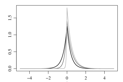
Figure 1: Shapes of asymmetric Laplace densities. The black line is the ALD density when $q=0.5$ and $\tau=0.2$, the darker grey line is for $q=0.3$ and $\tau=0.15$, and the lightest grey line is for $q=0.1$ and $\tau=0.05$.

The asymmetric Laplace distribution is a flexible model for unimodal distributions with the Laplace distribution being a special case. It is more peaked at zero than a normal distribution, but also can reflect the potential skewness of the distribution of true effects that often exists in applications, for example, in cases where more $\theta_{i}$’s are positive than negative, or vice versa. For multiple testing problems were we expect that most $\theta_{i}$’s are close to zero, it is natural to consider only submodels where $\mu=0$. In this case, method of moment estimates for the scale and skew parameters may be obtained from the first and second sample moments of ${\boldsymbol{Y}}$. Under the hierarchical model, we have

$${\text{E}}[Y]={\text{E}}[{\text{E}}[Y|\theta]]={\text{E}}[\theta]=\frac{\tau(1-2q)}{q(1-q)},$$

$${\text{Var}}[Y]={\text{E}}[{\text{Var}}[Y|\theta]]+{\text{Var}}[{\text{E}}[Y|\theta]]=1+{\text{Var}}[\theta]=1+\frac{\tau^{2}(1-2q+2q^{2})}{(1-q)^{2}q^{2}}.$$

By setting

$$\begin{split}&\frac{1}{m}\sum Y_{i}=\frac{\tau(1-2\hat{q})}{\hat{q}(1-\hat{q})},\\ &\frac{1}{m-1}\sum(Y_{i}-\bar{y})=1+\frac{\hat{\tau}^{2}(1-2\hat{q}+2\hat{q}^{2})}{(1-\hat{q})^{2}\hat{q}^{2}},\end{split}$$

we can solve for $\hat{q}$ and $\hat{\tau}$ to obtain moment-based estimates of $q$ and $\tau$.

3 Simulation Studies

In this section we use several simulation scenarios to compare the performance of Benjamini and Yekutieli’s procedure (BY), the loose control procedure (LC), and a tight control empirical procedure using an asymmetric Laplace model for the $\theta_{i}$’s (TCEA). For each simulation scenario, 1000 datasets were simulated as follows: First, values $\theta_{1},\ldots,\theta_{m}$ were independently simulated from a distribution $G$. Then an observation vector $\boldsymbol{Y}$ was sampled from a $N(\boldsymbol{\theta},\boldsymbol{I})$ distribution. For each of these datasets, the sign error proportions and the total numbers of signs inferred by each procedure were calculated. For all procedures and simulation scenarios the target level $\alpha_{S}$ was set to be 10%. Simulations were run for $q\in\{0.1,0.3,0.5\}$ and for five different values of $\tau$ for each level of $q$. The ranges of the $\tau$ values were chosen so that SEP ranged between $10\%$ to $30\%$ when the experimentwise type I error rate $\alpha=0.05$.

The results for several simulation scenarios with $m=5000$ are summarized in Figure 2. Overall, the TCEA procedure performs nearly as well as the TCO procedure. Both procedures control SEP at the prespecified level $\alpha_{S}=0.1$, and infer many more signs than the BY and LC procedures, with BY being the least powerful of the three. The difference between TCEA and LC or BY becomes larger as $\tau$ increases.

Figure 2: Comparison of the three procedures when $m=5000$ and the $\theta_{i}$’s have an asymmetric Laplace distribution. The skewness parameter $q$ is set to be 0.1 in the left column, 0.3 in the middle column, and 0.5 in the right column. Vertical bars around each plotting character correspond to $\pm 1.96$ Monte Carlo standard errors.

When number of experiments is large, the TCEA procedure is very close to the TCO procedure as our asymptotic result predicts. However, when $m=100$, TCEA and TCO show some differences. The results for several simulations with $m=100$ are summarized in Figure 3. In this situation, TCEA still performs better than BY or LC in terms of the power to infer signs. Also, we see that for some cases, the SEP of the oracle procedure does not attain the nominal level of 0.1. This is because tight control procedure is designed to keep MSER under the nominal level $\alpha_{s}$. As illustrated before, controlling MSER under $\alpha_{S}$ gives an accurate control over the expected SEP when $m$ is large. When $m$ is small, the probability of making no rejections across all experiments is non-negligible, and MSER is slightly larger than expectation of SEP. In this case, instead of keeping the average SEP at $\alpha_{S}$, TCO keeps it under $\alpha_{S}$, making the result slightly conservative.

Figure 3: Comparison of the four procedures under the same settings as in Figure 2 but $m=100$.

Finally, we study the situation when $G$ is a spike and slab distribution. The spike is a unimodal distribution with mean zero and small variance, and the slab is a uniform distribution. For two asymmetric cases ($q\in\{0.1,0.3\}$) the slab is the uniform distribution on (2,4). For the symmetric case ($q=0.5$), the slab is the uniform distribution on $(-4,-2)\cup(2,4)$. In each case, the proportion of $\theta_{i}$’s that are sampled from the slab is $1\%$. Comparisons of the three procedures and TCO are summarized in Figure 4. As expected, the LC procedure overall has better performance than the BY and TCEA procedures. As the variance of the spike grows larger, the differences between the $\theta$-values sampled from the spike and the $\theta$-values sampled from the slab becomes smaller, and the multimodal spike and slab distribution becomes closer and closer to a unimodal distribution that can be well-represented by a member of the asymmetric Laplace family. In such scenarios, TCEA does well in terms of maintaining MSER and inferring signs.

Figure 4: Comparisons of the three procedures when $m=5000$ and under a spike and slab distribution for the $\theta_{i}$’s. From left to right, the spike is sampled from an asymmetric Laplace distribution with $q=0.1,0.3,0.5$, respectively.

4 MSER and MSDR Optimization Subject to Type I Error Control

We have discussed controlling MSER under a prespecified level by choosing an appropriate significance threshold. In this section, we study the relationship between MSER and the shape of the acceptance region when the level $\alpha$ for the experimentwise type I error rate is held fixed. We show how to minimize the MSER while maintaining the experimentwise type I error rate. Storey (2007) has proposed a general framework for maximizing the statistical power of a test while maintaining the experimentwise type I error rate. Wasserman and Roeder (2006) and Dobriban et al. (2015) studied a weighted Bonferroni method to control family-wise type I error rate while maximizing the power. As illustrated in Gelman and Carlin (2014) and Owen (2016), a high sign error rate occurs when the error variance is large compared to the true effect size. We show that other than the error variance, the shape of the acceptance region is another crucial factor in determining the sign error rate.

In addition to MSER, we define the Marginal Sign Discovery Rate (MSDR) as $\text{MSDR}=\Pr(R_{1}=1)$. This quantity measures the expected proportion of the number of experiments with a sign inferred among all of the experiments since

$$\text{MSDR}=\Pr(R_{1}=1)=\frac{\sum_{i=1}^{m}\Pr(R_{i}=1)}{m}=\frac{\sum_{i=1}^{m}{\text{E}}[\textbf{1}(R_{i}=1)]}{m}=\frac{{\text{E}}[\sum_{i=1}^{m}\textbf{1}(R_{i}=1)]}{m}=\text{E}\left[\frac{R}{m}\right].$$

Both MSER and MSDR are affected by the acceptance region of the test. The usual acceptance region for each $H_{i}$ is $A=(\Phi^{-1}(\alpha/2),\Phi^{-1}(1-\alpha/2))$, which corresponds to the uniformly most accurate unbiased (UMAU) test. Following the ideas of Yu and Hoff (2016), we can construct a class of acceptance regions that corresponds to all level $\alpha$ two-sided tests $A(\alpha,s)=\{Y_{i}:\Phi^{-1}(\alpha s)<Y_{i}<\Phi^{-1}(1-\alpha(1-s))\}$, where $s\in(0,1)$ is a constant. Thus even if the level $\alpha$ is fixed, we can change the acceptance region by varying its endpoints. When $s<1/2$, the acceptance region tends to cover more negative observations and less positive observations. When $s>1/2$, the acceptance region tends to cover more positive observations and less negative observations. As $s\to 0$ or $1$, the two-sided test converges to a one-sided test with an acceptance region of either $(\Phi^{-1}(\alpha),\infty)$ or $(-\infty,\Phi^{-1}(1-\alpha))$. We now examine which $s$ value minimizes MSER and which $s$ value maximizes MSDR when the experimentwise type I error rate $\alpha$ is held fixed. Similar to (4), we can express the MSER as

$$\begin{split}\text{MSER}(A(\alpha,s))&=\frac{E[B_{1}\textbf{1}(\theta_{1}>0)+B_{2}\textbf{1}(\theta_{1}<0)]}{E[B_{1}+B_{2}]},\\ \text{MSDR}(A(\alpha,s))&=E[B_{1}+B_{2}],\end{split}$$

where $B_{1}=\Phi(\Phi^{-1}(\alpha s)-\theta)$ and $B_{2}=\Phi(\Phi^{-1}(\alpha(1-s))+\theta)$.

If we fix $\alpha$, MSER and MSDR can be seen as function of $s$. Under our models, we turn the minimization of MSER and maximization of MSDR into two one-parameter optimization problems: Denote

$$\begin{split}s^{D}&=\text{arg}\max_{s}\text{MSDR}(s)\\ s^{E}&=\text{arg}\min_{s}\text{MSER}(s).\end{split}$$

Interestingly the UMAU procedure, where $s=s^{U}=1/2$, does not always maximize the expected power, and the $s$ that maximizes the MSDR does not necessarily minimizes the MSER, vice-versa. We use a simple numerical example to illustrate this. Suppose $\theta_{i}$’s are sampled from a shifted chi-square distribution $\chi^{2}_{3}-3$. By numerical evaluation, the results are summarized in Table 1.

	$s$ value	$A(s,0.05)$	MSER($\%$)	MSDR
$s^{U}$	0.5	(-3.92, 3.92)	3.01	0.189
$s^{D}$	0.683	(-3.65, 4.30)	2.79	0.193
$s^{E}$	0.829	(-3.45, 4.80)	2.71	0.190

Table 1: Comparison of the usual acceptance region, the acceptance region that maximizes MSDR, and the acceptance region that minimizes MSER

On the other hand, Storey (2007) noticed that when $\theta\sim N(0,\sigma_{b}^{2})$, the test that maximizes expected power is the UMAU test. Here we prove a more general theorem that the UMAU test actually both maximizes expected power and minimizes MSER when the distribution of $\theta$ is symmetric.

Proposition 4.1.

If $G$ is a distribution that is symmetric with respect to 0, the two-sided test that maximizes MSDR and minimizes the MSER is the UMAU test, i.e. $s^{D}=s^{E}=1/2$.

Thus in applications where $\alpha$ is held fixed, if we believe that the distribution of the $\theta_{i}$’s is symmetric, we should use the usual acceptance region. In situations where we suspect this distribution to be asymmetric, then using either $S^{D}$ or $S^{E}$ can lead to a test with either higher MSDR or lower MSER. However, identifying $S^{D}$ or $S^{E}$ requires $G$ to be known. Similar to the TCE procedure, in practice we replace $G$ with an estimate $\hat{G}$ and obtain empirical estimates $\widehat{\text{MSDR}}$ and $\widehat{\text{MSER}}$, and then obtain $S^{D}$ or $S^{E}$ by maximizing $\widehat{\text{MSDR}}$ or minimizing $\widehat{\text{MSER}}$.

5 Discussion

In this article, we use the MSER as a measure of sign errors in multiple testing settings. We proposed two types of procedures to control MSER, loose control procedure and tight control procedure. Loose control procedure can be conservative but is robust to the distribution of the $\theta_{i}$’s, while the tight control procedure is more powerful but assumes the distribution of $\theta_{i}$’s is a member of a known parametric model.

The loose control procedure proposed in this paper is closely related to the BY procedure. Unlike the derivation for the BY procedure, we derive the LC procedure from the perspective of controlling the MSER, which is a quantity measuring the probability of making a sign error under a hierarchical model. We assume that there are no “true nulls” in this paper, because in many applications true nulls do not exist. By assuming no true nulls, the loose control procedure we derived is more powerful than the BY procedure in terms of the number of inferred signs. If it is believed that the true nulls do exist, the loose control procedure can still control the SER, although control over MSER depends on how we define a sign error when $\theta_{i}=0$. If we define that when $\theta_{i}=0$, either claiming $\theta$ is positive or negative is correct, the loose control procedure stays the same as proposed in this paper. If we define that when $\theta_{i}=0$, either claiming $\theta$ is positive or negative is wrong, then the BY procedure should be used since it also controls the mixed directional FDR, where any sign declaration of $\theta_{i}=0$ is considered as a sign error.

We also discussed varying the endpoints of the acceptance region to reduce MSER and increase MSDR when the type I error rate is fixed. This can be combined with the tight control procedure, leading to a new procedure: Choose $\alpha$ and $s$ such that

$$\begin{split}&(\alpha,s)=\arg\max_{(\alpha,s)}\widehat{MSDR}(A(\alpha,s))\\ &\text{such that\quad}\widehat{\text{MSER}}(A(\alpha,s))<\alpha_{S}.\end{split}$$

Given an estimate $\hat{G}$ of $G$, the solution for $(\alpha,s)$ can be obtained numerically. This procedure can potentially increase the power in inferring signs. However, the performance of this procedure is more unstable since the optimization task here is more complicated.

Appendix

Proof of Lemma 2.1.

Note that $(Y_{1},\theta_{1}),\ldots,(Y_{m},\theta_{m})$ are an i.i.d sample from the hierarchical model (1) and (2). For $H_{i}$, $\forall i\in\{1,...,m\}$, given that it is rejected, the probability of making a sign error is $\Pr(E_{i}=1|R_{i}=1)$, which is MSER as specified in (3). Given that $R=r$ hypotheses are rejected, the total number of sign errors should follow a binomial distribution, i.e. $E\;|R=r\sim Bi(r,\text{MSER})$. Thus $R\cdot\text{SEP}\;|R=r\sim Bi(r,\text{MSER})$. ∎

Proof of Proposition 2.1.

We just need to show that $\text{SEP}-\text{MSER}\to 0$ in probability, which is to show $\text{SEP}-{\text{E}}[\text{SEP}]+{\text{E}}[\text{SEP}]-\text{MSER}\to 0$ in probability. Since ${\text{E}}[\text{SEP}]=\text{MSER}\cdot\Pr(R>0)=\text{MSER}\cdot(1-\Pr(R_{1}=0)^{m})$, we have ${\text{E}}[\text{SEP}]\to\text{MSER}$ in probability as $m\to\infty$ (note $\Pr(R_{1}=0)<1$ in our setting). Now we just need to show that $\text{SEP}-{\text{E}}[\text{SEP}]\to 0$ in probability, which can be done by showing ${\text{E}}[(\text{SEP}-{\text{E}}[\text{SEP}])^{2}]\to 0$. We have

$$\begin{split}{\text{E}}[(\text{SEP}-{\text{E}}[\text{SEP}])^{2}]&={\text{Var}}[\text{SEP}]={\text{Var}}[{\text{E}}[\text{SEP}|R]]+{\text{E}}[{\text{Var}}[\text{SEP}|R]]\\ &={\text{Var}}[\text{MSER}\cdot\textbf{1}(R>0)]+{\text{E}}[\frac{R\cdot\text{MSER}(1-\text{MSER})}{R^{2}}\textbf{1}(R>0)]\\ &=\text{MSER}^{2}\cdot\Pr(R>0)(1-\Pr(R>0))+\text{MSER}(1-\text{MSER})\cdot{\text{E}}[\frac{1}{R}\textbf{1}(R>0)].\end{split}$$

The first part goes to 0 because $\Pr(R>0)\to 1$ as $m\to\infty$. The second part goes to 0 because $R$ follows a binomial distribution $Bi(m,\Pr(R_{1}=1))$, and

$$\begin{split}{\text{E}}[\frac{1}{R}\textbf{1}(R>0)]&<{\text{E}}[\frac{2}{R+1}\textbf{1}(R>0)]<2{\text{E}}[\frac{1}{R+1}\textbf{1}(R>0)]\\ &=2{\text{E}}[\frac{1}{R+1}]-2{\text{E}}[\frac{1}{0+1}\textbf{1}(R=0)]\\ &=\frac{2}{(m+1)\Pr(R_{1}=1)}\cdot(1-(1-\Pr(R_{1}=1))^{m+1})-2\Pr(R=0)\to 0\end{split}$$

as $m\to\infty$. Therefore, $\text{SEP}-\text{MSER}\to 0$ in probability. ∎

Before proving Proposition 2.2 and Proposition 2.3, we first prove the Lemma below.

Lemma 5.1.

Let $A(\alpha,s)=\{y:\Phi^{-1}(\alpha s)<y<\Phi^{-1}(1-\alpha(1-s))$. Let

$$\gamma(A(\alpha,s))=\text{E}_{G}[B_{1}(A(\alpha,s))\textbf{1}(\theta>0)+B_{2}(A(\alpha,s))\textbf{1}(\theta<0)],$$

we have that $\gamma(A(\alpha,s))\leq\alpha s\pi_{0}+\alpha(1-s)(1-\pi_{0})$, where $\pi_{0}=\Pr(\theta>0)$.

Proof.

Under the hierarchical model we have,

$$\gamma(A(\alpha,s))=\text{E}_{G}[\Phi(\Phi^{-1}(\alpha s)-\theta)\textbf{1}(\theta>0)+\Phi(\Phi^{-1}(\alpha(1-s))+\theta)\textbf{1}(\theta<0)].$$

Denote $\gamma(A(\alpha,s))=\gamma_{1}+\gamma_{2}$ where $\gamma_{1}=\text{E}_{G}[\Phi(\Phi^{-1}(\alpha s)-\theta)\textbf{1}(\theta>0)]$, and $\gamma_{2}=\text{E}_{G}[\Phi(\Phi^{-1}(\alpha(1-s))+\theta)\textbf{1}(\theta<0)]$. Suppose the probability density function of $G$ is $g$,for $\gamma_{1}$ we have

$$\begin{split}\gamma_{1}=&\text{E}_{G}[\Phi(\Phi^{-1}(\alpha s)-\theta)\textbf{1}(\theta\geq 0)]\\ &=\int_{0}^{\infty}\Phi(-\theta+\Phi^{-1}(\alpha s))g(\theta)d\theta\\ &=\Phi(-\theta+\Phi^{-1}(\alpha s))G(\theta)|^{\infty}_{0}+\int_{0}^{\infty}\phi(-\theta+\Phi^{-1}(\alpha s))G(\theta)d\theta\\ &=-\alpha s(1-\pi_{0})+\int_{0}^{\infty}\phi(-\theta+\Phi^{-1}(\alpha s))G(\theta)d\theta\\ &\leq-\alpha s(1-\pi_{0})+\int_{0}^{\infty}\phi(-\theta+\Phi^{-1}(\alpha s))d\theta\\ &=-\alpha s(1-\pi_{0})+\alpha s=\alpha s\pi_{0}\end{split}$$ (5)

For $\gamma_{2}$ we have

$$\begin{split}\gamma_{2}=&\text{E}_{G}[\Phi(\Phi^{-1}(\alpha(1-s))+\theta)\textbf{1}(\theta\leq 0)]\\ &=\int_{-\infty}^{0}\Phi(\theta+\Phi^{-1}(\alpha(1-s)))g(\theta)d\theta\\ &=\Phi(\theta+\Phi^{-1}(\alpha(1-s)))G(\theta)|_{-\infty}^{0}-\int^{0}_{-\infty}\phi(\theta+\Phi^{-1}(\alpha(1-s)))G(\theta)d\theta\\ &=\alpha(1-s)(1-\pi_{0})-\int^{0}_{-\infty}\phi(\theta+\Phi^{-1}(\alpha(1-s)))G(\theta)d\theta\\ &\leq\alpha(1-s)(1-\pi_{0})\end{split}$$ (6)

Therefore $E(A(\alpha,s))=\gamma_{1}+\gamma_{2}\leq\alpha s\pi_{0}+\alpha(1-s)(1-\pi_{0})$. ∎

Proof of Proposition 2.3.

Denote $R^{t}$ as the total number of rejections. We have

$${\text{E}}[R^{t}/m]={\text{E}}[\sum\textbf{1}(R_{j}=1)]/m=\sum\Pr(R_{j}=1)/m=\Pr(R_{i}=1),$$

where the last step is because of the exchangeability of the model. Again, we write $\text{MSER}=\gamma/\beta$, where $\gamma=\Pr(E_{i}=1,R_{i}=1)$ and $\beta=\Pr(R_{i}=1)$. Since $\alpha_{l}^{i}$ is independent of $Y_{i}$, and by Lemma 5.1 and letting $s=1/2$, we have

$$\Pr(E_{i}=1,R_{i}=1|\alpha_{l}^{i})\leq\alpha_{l}^{i}/2\leq\alpha_{S}((R(\alpha_{l}^{i})-1)\vee 0)/m\leq\alpha_{S}R^{t}/m.$$

Thus $\gamma={\text{E}}[\Pr(E_{i}=1,R_{i}=1|\alpha_{l}^{i})]\leq\alpha_{S}{\text{E}}[R^{t}/m]=\alpha_{S}\beta$. Therefore $\text{MSER}\leq\alpha_{S}$. ∎

Proof of Proposition 2.4.

This Proposition follows from Benjamini and Yekutieli (2005) Theorem 1 and Corollary 3. To modify the proof for LC procedure, we should replace the $kq/m$ in equation (4) in Benjamini and Yekutieli (2005) with $2kq/m$. Then it is easy to see that the SER can be controlled under $q$, which is the $\alpha_{S}$ we have in this paper. Since LC is more conservative than LC, NLC also controls SER below $\alpha_{S}$. ∎

Proof of Proposition 2.2.

This is implied by Proposition 2.4. Note that when $m\to\infty$, $\text{SER}-\text{MSER}\to 0$ in probability according to the proof of Proposition 2.1, hence MSER $<\alpha_{s}$ in probability. ∎

Proof of Proposition 2.5.

We first show that $\widehat{\text{MSER}}\stackrel{{\scriptstyle p}}{{\rightarrow}}\text{MSER}$. Since both $B_{1}$ and $B_{2}$ are integrable and the probability density function $g_{\eta}$ of $G$ is continuous in $\eta$, $\text{E}_{G}[B_{1}+B_{2}]=\int(B_{1}+B_{2})g_{\eta}(\theta)d\theta$ is a continuous function of $\eta$ and it is always nonzero. Similarly, $\text{E}_{G}[B_{1}\textbf{1}(\theta\geq 0)+B_{2}\textbf{1}(\theta\leq 0)]$ is a continuous function in $\eta$. Therefore, MSER is a continuous function in $\eta$. Note that the difference between MSER and $\widehat{\text{MSER}}$ is that the former uses $\eta$ and the later uses $\hat{\eta}$. If $\hat{\eta}\stackrel{{\scriptstyle p}}{{\rightarrow}}\eta$, then we have $\widehat{\text{MSER}}\to\text{MSER}$ by Continuous Mapping Theorem.

Since $\alpha_{o}$ is the unique solution such that $\text{MSER}(A(\alpha_{o}))-\alpha_{S}=0$, and $\alpha^{e}$ is the unique solution such that $\widehat{\text{MSER}}(A(\alpha_{e}))-\alpha_{e}=0$, we have $\alpha_{e}\stackrel{{\scriptstyle p}}{{\rightarrow}}\alpha_{o}$ by M-estimator theory (Lemma 5.10, Van der Vaart (1998)).

∎

Proof of Proposition 4.1.

We first show that $s=1/2$ maximizes the MSDR. The MSDR can be written as

$$\begin{split}\text{MSDR}(s)&=\int_{-\infty}^{\infty}(B_{1}(\theta,s)+B_{2}(\theta,s))g(\theta)d\theta\\ &=\int_{-\infty}^{0}(B_{1}(\theta,s)+B_{2}(\theta,s))g(\theta)d\theta+\int_{0}^{\infty}(B_{1}(\theta,s)+B_{2}(\theta,s))g(\theta)d\theta\end{split}$$

Since $g$ is symmetric,

$$\begin{split}\text{MSDR}(s)&=\int_{0}^{\infty}(B_{1}(-\theta,s)+B_{2}(-\theta,s))g(\theta)d\theta+\int_{0}^{\infty}(B_{1}(\theta,s)+B_{2}(\theta,s))g(\theta)d\theta\\ &=\int_{0}^{\infty}((B_{1}(\theta,s)+B_{2}(\theta,s)+B_{1}(-\theta,s)+B_{2}(-\theta,s))g(\theta)d\theta\end{split}$$

Now we prove that the integrand is maximized when $s=1/2$, which does not depend on $\theta$. Thus $\text{MSDR}(s)$ is maximized when $s=1/2$. The integrand can be written as $H(s)g(\theta)$ where

$$H(s)=\Phi(\Phi^{-1}(\alpha s)-\theta)+\Phi(\Phi^{-1}(\alpha(1-s))+\theta)+\Phi(\Phi^{-1}(\alpha s)+\theta)+\Phi(\Phi^{-1}(\alpha(1-s))-\theta)$$ (7)

Taking the derivative with respect to $s$, we have

$$\begin{split}H(s)^{\prime}&=\frac{\phi(\Phi^{-1}(\alpha s)-\theta)}{\phi(\Phi^{-1}(\alpha s))}+\frac{\phi(\Phi^{-1}(\alpha s)+\theta)}{\phi(\Phi^{-1}(\alpha s))}-\frac{\phi(\Phi^{-1}(\alpha(1-s))-\theta)}{\phi(\Phi^{-1}(\alpha(1-s)))}-\frac{\phi(\Phi^{-1}(\alpha(1-s))+\theta)}{\phi(\Phi^{-1}(\alpha(1-s)))}\\ &=c_{1}(exp(\Phi^{-1}(\alpha s)\theta)+exp(-\Phi^{-1}(\alpha s)\theta)-exp(\Phi^{-1}(\alpha(1-s))\theta)-exp(-\Phi^{-1}(\alpha(1-s))\theta)),\end{split}$$ (8)

where $c_{1}$ is a positive constant. It’s easy to see that $s=1/2$ is one solution to $H(s)^{\prime}=0$. Now we show that $H(s)$ is actually concave, hence $s=1/2$ maximizes $H(s)$ for every $\theta>0$. Therefore $s=1/2$ maximizes $\text{MSDR}(s)$. By taking derivative of $H(s)^{\prime}$ with respect to $s$ and rearrange, we obtain

$$\begin{split}H(s)^{\prime\prime}&=c_{2}(exp((\Phi^{-1}(\alpha s)+\theta)^{2}/2)+exp((\Phi^{-1}(\alpha(1-s))+\theta)^{2}/2)-exp((\Phi^{-1}(\alpha s)-\theta)^{2}/2)\\ &\quad\quad-exp((\Phi^{-1}(\alpha(1-s))-\theta)^{2}/2)),\end{split}$$

where $c_{2}$ is a positive constant. Since $\Phi^{-1}(\alpha s)<0$ and $\theta>0$ (the integral is from 0 to $\infty$), we have

$$|\Phi^{-1}(\alpha s)-\theta|=|\Phi^{-1}(\alpha s)|+|\theta|\geq|\Phi^{-1}(\alpha s)+\theta|.$$

Thus

$$exp((\Phi^{-1}(\alpha s)+\theta)^{2}/2)-exp((\Phi^{-1}(\alpha s)-\theta)^{2}/2)<0.$$

Similarly

$$exp((\Phi^{-1}(\alpha(1-s))+\theta)^{2}/2)-exp((\Phi^{-1}(\alpha(1-s))-\theta)^{2}/2)<0.$$

Therefore $H(s)^{\prime\prime}<0$, and $s=1/2$ maximizes $\text{MSDR}(s)$.

To show MSER is minimized by $1/2$, we can first show that $s=1/2$ minimizes $\gamma$, using the same technique as previous part of this proof. Then by noticing that $\text{MSER}=\gamma/\text{MSDR}$, we know $s=1/2$ minimizes MSER. ∎

References

• Benjamini (2010) Benjamini, Y. (2010). Discovering the false discovery rate. Journal of the Royal Statistical Society: Series B (Statistical Methodology)Β 72(4), 405–416.
• Benjamini and Hochberg (1995) Benjamini, Y. and Y.Β Hochberg (1995). Controlling the false discovery rate: a practical and powerful approach to multiple testing. Journal of the royal statistical society. Series B (Methodological), 289–300.