Frequency-driven market mechanisms for optimal dispatch in power networks

Abstract

This paper studies real-time bidding mechanisms for economic dispatch and frequency regulation in electrical power networks. We consider a market administered by an independent system operator (ISO) where a group of strategic generators participate in a Bertrand game of competition. Generators bid prices at which they are willing to produce electricity. Each generator aims to maximize their profit, while the ISO seeks to minimize the total generation cost and to regulate the frequency of the system. We consider a continuous-time bidding process coupled with the swing dynamics of the network through the use of frequency as a feedback signal for the negotiation process. We analyze the stability of the resulting interconnected system, establishing frequency regulation and the convergence to a Nash equilibrium and optimal generation levels. The results are verified in the IEEE 14-bus benchmark case.

I Introduction

Power generation dispatch is typically done in a hierarchical fashion, where the different layers are separated according to their time scales. Broadly, at the top layer economic efficiency is ensured via market clearing and at the bottom layer frequency control and regulation is achieved via primary and secondary controllers. However, the intermittent and uncertain nature of distributed energy resources (DERs) and their integration into the power grid represents a major challenge to the current design. Of particular concern is the need to maintain both frequency regulation and cost efficiency of regulation reserves in the face of increasing fluctuations in renewables. To this end, we propose an integrated dynamic market mechanism which combines the real-time market and frequency regulation, allowing competitive market players, including renewable generation, to negotiate electricity prices while using the most recent information on the grid frequency.

Literature review

The combination of economic dispatch and frequency regulation has received increasing attention in recent years. Various works have sought to move beyond the traditional and compartmentalized hierarchical control layers to instead simultaneously achieve frequency stabilization and economic dispatch in power networks [2, 3, 4] and microgrids [5, 6]. Along this line of research, the various agents involved work cooperatively towards the satisfaction of a common goal. An alternative body of research has investigated the use of price-based incentives for economic generation- and demand-side management and frequency regulation [7, 8, 9]. To achieve these goals, these works consider dynamic pricing mechanisms in conjunction with system dynamics of the power network. We also adopt this approach, with the important distinction that here we allow generators to bid in the market (hence, they are price-setters rather than price-takers). This viewpoint results in a Bertrand game of competition among the generators. Our previous work [10, 11] studied this type of games established that iterative bidding can achieve convergence to an optimal allocation of power generation, without considering the effects on the dynamics of the power network. The underlying assumption was that generation setpoints could be commanded after convergence, which in practice poses a limitation, considering the fast time-scales at which DERs operate. Instead, this paper proposes an online bidding scheme where the setpoints are updated continuously throughout time to better cope with fast changes in the network. In this way, we tackle simultaneously both frequency regulation, optimal power dispatch and the competitive aspect among the generators.

Statement of contributions

We consider an electrical power network consisting of an independent system operator (ISO) and a group of competitive generators. Each generator seeks to maximize its individual profit, while the ISO aims to solve the economic dispatch problem and regulate the frequency. Since the generators are not willing to share their cost functions, the ISO is unable to solve the economic dispatch problem. Instead, it has the generators compete in a bidding market where they submit bids to the ISO in the form of a price at which they are willing to produce electricity. In return, the ISO determines the power generations levels the generators have to meet. We analyze the underlying Bertrand game among the generators and characterize the Nash equilibria that correspond to optimal power dispatch termed efficient Nash equilibria. In particular, we establish the existence of such efficient Nash equilibria and provide a sufficient condition for its uniqueness. We also propose a Nash equilibrium seeking scheme in the form of a continuous-time bidding process that captures the interaction between the generators and the ISO. In this scheme, the generators adjust their bid based on their current bid and the production level that the ISO requests from them with the aim to maximize their profit. At the same time, the ISO adjusts the generation setpoints to minimize the total payment to the generators while taking the power balance and frequency deviation into account. Moreover, along the execution of the algorithm the nonnegativity constraints on the bids and power generation quantities are satisfied. The use of the local frequency error as a feedback signal in the negotiation process couples the ISO-generator coordination scheme with the swing dynamics of the power network. We show that each equilibrium of the interconnected system corresponds to an efficient Nash equilibrium, optimal generation levels and zero frequency regulation. We furthermore establish local convergence to such an equilibrium by invoking a suitable invariance principle for the closed-loop projected dynamical system. Finally, the numerical results on the IEEE 14-bus benchmark show fast convergence of the closed-loop system to an optimal equilibrium, even under sudden changes of the load and the cost functions.

Notation

Let $\mathbb{R},\mathbb{R}_{\geq 0},\mathbb{R}_{>0}$ be the set of real, nonnegative real, and positive real numbers, respectively. We write the set $\{1,\ldots,n\}$ compactly as $[n]$. We denote by $\mathds{1}\in\mathbb{R}^{n}$ the vector whose elements are equal to 1. Given a twice differentiable function $f:{}^{n}\rightarrow\real$, its gradient and its Hessian evaluated at $x$ is written as $\nabla f(x)$ and $\nabla^{2}f(x)$, respectively. A twice continuously differentiable function $f:{}^{n}\rightarrow\real$ is strongly convex on $S\subset{}^{n}$ if it is convex and, for some $\mu>0$, its Hessian satisfies $\nabla^{2}f(x)>\mu I$ for all $x\in S$. For scalars $a,b\in\mathbb{R}$ we denote by $[a]^{+}_{b}$ the operator

$$[a]^{+}_{b}=\begin{cases}a&\text{if }b>0\\ \max(a,0)&\text{if }b=0.\end{cases}$$ (1)

For vectors $a,b\in{}^{n}$, $[a]^{+}_{b}$ denotes the vector whose $i$-th element is given by $[a_{i}]^{+}_{b_{i}}$ for $i\in[n]$. For $A\in\mathbb{R}^{m\times n}$, the induced $2$-norm is denoted by $\|A\|$. Given $v\in\mathbb{R}^{n},\tau\in\mathbb{R}^{n\times n}$, we write $\|v\|_{\tau}:=\sqrt{v^{T}\tau v}$. Given a set of numbers $v_{1},v_{2},\ldots,v_{n}\in\real$, $\operatorname{col}(v_{1},\ldots,v_{n})$ denotes the column vector $\begin{bmatrix}v_{1},\dots,v_{n}\end{bmatrix}^{T}$ and likewise $\operatorname{diag}(v_{1},\ldots,v_{n})$ denotes the $n\times n$ diagonal matrix with entries $v_{1},\ldots,v_{n}$ on the diagonal. For $u,v\in\mathbb{R}^{n}$ we write $u\perp v$ if $u^{T}v=0$. We use the compact notational form $0\leq u\perp v\geq 0$ to denote the complementarity conditions $u\geq 0,v\geq 0,u\perp v$. The notations $\operatorname{\mathbf{sin}}(.)$ and $\operatorname{\mathbf{cos}}(.)$ are used to represent the element-wise sine and cosine functions respectively.

II Power network model and dynamics

We consider an electrical power network consisting of $n$ buses and $m$ transmission lines. The network is represented by a connected and undirected graph $\mathcal{G}=(\mathcal{V},\mathcal{E})$, where nodes $\mathcal{V}=[n]$ represent buses and edges $\mathcal{E}\subset\mathcal{V}\times\mathcal{V}$ are the transmission lines connecting the buses. The edges are arbitrarily labeled with a unique identifier in $[m]$ and the ends of each edge are arbitrary labeled with ‘+’ and ‘-’. The incidence matrix $D\in{}^{n\times m}$ of the resulting directed graph is

$$D_{ik}=\begin{cases}+1&\text{if $i$ is the positive end of edge $k$},\\ -1&\text{if $i$ is the negative end of edge $k$},\\ 0&\text{otherwise.}\end{cases}$$

Each bus $i$ represents a control area and is assumed to have one generator and a load $P_{di}$. The dynamics at the buses is assumed to be governed by the swing equations [12], given by

$$\dot{\delta} =\omega$$ (2)

$$M\dot{\omega} =-D\Gamma\operatorname{\mathbf{sin}}(D^{T}\delta)-A\omega+P_{g}-P_{d}$$

with $P_{d}=\operatorname{col}(P_{d1},\ldots,P_{dn})$. Here $\Gamma=\operatorname{diag}(\gamma_{1},\ldots,\gamma_{m})$, where $\gamma_{k}=B_{ij}V_{i}V_{j}=B_{ji}V_{i}V_{j}$ and $k\in[m]$ corresponds to the edge between nodes $i$ and $j$. Table I presents a list of symbols employed in the model (2).

$$\delta \in\mathbb{R}^{n}$$ voltage phase angle

$$\omega \in\mathbb{R}^{n}$$ frequency deviation w.r.t. the nominal frequency

$$P_{g} \in{\mathbb{R}}_{\geq 0}^{n}$$ power generation

$$P_{d} \in{\mathbb{R}}_{\geq 0}^{n}$$ power load

$$M \in\mathbb{R}_{\geq 0}^{n\times n}$$ diagonal matrix of moments of inertia

$$A \in{\mathbb{R}}_{\geq 0}^{n\times n}$$ diagonal matrix of asynchronous damping constants

$$V_{i} \in\mathbb{R}_{>0} \text{voltage magnitude at bus }i$$

$$B_{ij} \in\mathbb{R}_{>0} \text{negative of the susceptance of transmission line }(i,j)$$

Table I: State variables and parameters of swing equations (2).

For the stability analysis carried out later, it is convenient to work with the voltage phase angle differences $\varphi=D_{t}^{T}\delta\in\mathbb{R}^{n-1}$. Here $D_{t}\in\mathbb{R}^{n\times(n-1)}$ is the incidence matrix of an arbitrary tree graph on the set of buses $[n]$ (e.g., a spanning tree of the physical network). Furthermore, let $U(\varphi)=-\mathds{1}^{T}\Gamma\operatorname{\mathbf{cos}}(D^{T}D_{t}^{\dagger T}\varphi)$, where $D_{t}^{\dagger}=(D_{t}^{T}D_{t})^{-1}D_{t}^{T}$ denotes the Moore-Penrose pseudo-inverse of $D_{t}$. Then the physical system (2) in the $(\varphi,\omega)$-coordinates takes the form

$$\dot{\varphi} =D_{t}^{T}\omega$$ (3)

$$M\dot{\omega} =-D_{t}\nabla U(\varphi)-A\omega+P_{g}-P_{d},$$

where we observe that $D_{t}D_{t}^{\dagger}D=(I-\frac{1}{n}\mathds{1}\mathds{1}^{T})D=D$.

III Problem description

In this section we formulate the problem statement, introduce the necessary game-theoretic tools and discuss the goals of the paper.

III-A ISO-generator coordination

Taking as starting point the electrical power network model described in Section II, here we outline the elements of the ISO-generator coordination problem following the exposition of [10, 11]. Let $C_{i}:{\mathbb{R}}_{\geq 0}\rightarrow{\mathbb{R}}_{\geq 0}$ be the cost incurred by generator $i\in[n]$ in producing $P_{gi}$ units of power. We assume $C_{i}$ is strongly convex on the domain ${\mathbb{R}}_{\geq 0}$ and satisfies $\nabla C_{i}(0)\geq 0$. Given the total network cost

$$C(P_{g}):=\sum_{i\in[n]}C_{i}(P_{gi})$$ (4)

and a power load $P_{d}$, the ISO seeks to solve the economic dispatch (ED) problem

$$\operatorname{minimize} \quad C(P_{g}),$$ (5a)

$$\operatorname{subject\text{$\,\,$}to} \quad\mathds{1}^{T}P_{g}=\mathds{1}^{T}P_{d},$$ (5b)

$$\quad P_{g}\geq 0,$$ (5c)

and, at the same time, to regulate the frequency of the physical power network. We assume the total load to be positive, i.e., $\mathds{1}^{T}P_{d}>0$ such that (5) is feasible. Since the constraints (5b) (5c) are affine, Slater’s condition holds implying that (5) has zero duality gap. We can also show that its primal-dual optimizer $(P_{g}^{*},\lambda^{*},\mu^{*})$ is unique by exploiting strong convexity of $C$. We assume that for the power injection $P_{g}=P_{g}^{*}$, there exists an equilibrium $(\bar{\varphi},\bar{\omega})$ of (3) that satisfies $D^{T}D_{t}^{\dagger T}\bar{\varphi}\in(-\pi/2,\pi/2)^{m}$. The latter assumption is standard and is referred to as the security constraint in the power systems literature [12].

We note that the ISO cannot determine the optimizer of the ED problem (5) because generators are strategic and they do not reveal their cost functions to anyone. Instead, the ISO operates a market where each generator $i\in[n]$ submit a bid $b_{i}\in{\mathbb{R}}_{\geq 0}$ in the form of a price at which it is willing to provide power. Based on these bids, the ISO aims to find the power allocation that meets the load and minimizes the total payment to the generators. Thus instead of solving the ED problem (5) directly, the ISO considers, given a bid $b\in{\mathbb{R}}_{\geq 0}^{n}$, the convex optimization problem

$$\operatorname{minimize} \quad b^{T}P_{g},$$ (6a)

$$\operatorname{subject\text{$\,\,$}to} \quad\mathds{1}^{T}P_{g}=\mathds{1}^{T}P_{d},$$ (6b)

$$\quad P_{g}\geq 0.$$ (6c)

A fundamental difference between (5) and (6) is that the latter optimization is linear and may in general have multiple solutions. Let $P_{g}^{\text{opt}}(b)$ be the optimizer of (6) the ISO selects given bids $b$ and note that this might not be unique. Knowing the ISO’s strategy, each generator $i$ bids a quantity $b_{i}\geq 0$ to maximize its payoff

$$\Pi_{i}(b_{i},P_{gi}^{\text{opt}}(b)):=P_{gi}^{\text{opt}}(b)b_{i}-C_{i}(P_{gi}^{\text{opt}}(b)),$$ (7)

where $P_{gi}^{\text{opt}}(b)$ is the $i$-th component of the optimizer $P_{g}^{\text{opt}}(b)$. Note that this function is not continuous in the bid $b$. Since each generator is strategic, we analyze the market clearing, and hence the dispatch process explained above using tools from game theory [13, 14].

III-B Inelastic electricity market game

We define the inelastic electricity market game as

• Players: the set of generators $[n]$.

• Action: for each player $i$, the bid $b_{i}\in{\mathbb{R}}_{\geq 0}$.

• Payoff: for each player $i$, the payoff $\Pi_{i}$ defined in (7).

In the sequel we interchangeably use the notation $b\in{\mathbb{R}}_{\geq 0}^{n}$ and $(b_{i},b_{-i})\in{\mathbb{R}}_{\geq 0}^{n}$ for the bid vector, where $b_{-i}\in{\mathbb{R}}_{\geq 0}^{n-1}$ represents the bids of all players except $i$. We note that the payoff of generator $i$ not only depends on the bids of the other players but also on the optimizer $P_{g}^{\text{opt}}(b)$ the ISO selects. Therefore, the concept of a Nash equilibrium is defined slightly differently compared to the usual one.

Definition III.1 (Nash equilibrium [11]).

A bid profile $b^{*}\in{\mathbb{R}}_{\geq 0}^{n}$ is a Nash equilibrium of the inelastic electricity market game if there exists an optimizer $P_{g}^{\text{opt}}(b^{*})$ of (6) such that for each $i\in[n]$,

$$\Pi_{i}(b_{i},P_{gi}^{\text{opt}}(b_{i},b_{-i}^{*}))\leq\Pi_{i}(b_{i}^{*},P_{gi}^{\text{opt}}(b^{*}))$$

for all $b_{i}\in{\mathbb{R}}_{\geq 0}$ with $b_{i}\neq b_{i}^{*}$ and all optimizers $P_{gi}^{\text{opt}}(b_{i},b_{-i}^{*})$ of (6) given bids $(b_{i},b_{-i}^{*})$.

We are particularly interested in bid profiles for which the optimizer of (5) is also a solution to (6). This is captured in the following definition.

Definition III.2 (Efficient bid and efficient Nash equilibrium).

An efficient bid of the inelastic electricity market is a bid $b^{*}\in{\mathbb{R}}_{\geq 0}^{n}$ for which the optimizer $P_{g}^{*}$ of (5) is also an optimizer of (6) given bids $b=b^{*}$ and

$$P_{gi}^{*}=\operatorname*{arg\,max}_{P_{gi}\geq 0}\{P_{gi}b^{*}_{i}-C_{i}(P_{gi})\}\ \text{ for each }i\in[n].$$ (8)

A bid $b^{*}\in{\mathbb{R}}_{\geq 0}^{n}$ is an efficient Nash equilibrium of the inelastic electricity market game if it is an efficient bid and a Nash equilibrium.

At the efficient Nash equilibrium, the optimizer of the ED problem coincides with the production levels that maximize the individual profits (7) of the generators. This justifies studying the efficient Nash equilibria.

III-C Paper objectives

Given the problem setup described above, neither the ISO nor the individual strategic generators are able to determine the efficient Nash equilibrium a priori. As a first objective, we are interested in designing a Nash equilibrium seeking mechanism in the form of a bidding process where the generators coordinate with the ISO to dynamically update their bids and production levels, while respecting the nonnegativity constraints throughout its execution. Our second objective is the characterization of the stability properties of the interconnection of the bidding process with the physical dynamics of the power network.

IV Existence and uniqueness of Nash equilibria

In this section we establish existence of an efficient Nash equilibrium and also provide a condition for its uniqueness. While [11] has established the existence of one specific efficient Nash equilibrium, we provide in the following result a characterization of all efficient Nash equilibria.

Proposition IV.1.

(Characterization of efficient Nash equilibria): Let $(P_{g}^{*},\lambda^{*},\mu^{*})$ be the unique primal-dual optimizer of (5), that is, $P_{g}^{*}\in{}^{n},\lambda^{*}\in\real,\mu^{*}\in{}^{n}$ satisfy the Karush-Kuhn-Tucker (KKT) conditions

$$\begin{aligned} \nabla C(P_{g}^{*})&=\mathds{1}\lambda^{*}+\mu^{*},\qquad\mathds{1}^{T}P_{g}^{*}=\mathds{1}^{T}P_{d},\\ 0&\leq P_{g}^{*}\perp\mu^{*}\geq 0.\end{aligned}$$ (9)

Suppose $P_{gi}^{*}>0$ for at least two distinct generators. Then, any $b^{*}\in{\mathbb{R}}_{\geq 0}^{n}$ satisfying $\mathds{1}\lambda^{*}\leq b^{*}\leq\nabla C(P_{g}^{*})$ is an efficient Nash equilibrium of the inelastic electricity market game.

Proof.

Let $(P_{g}^{*},\lambda^{*},\mu^{*})$ satisfy (9), then in particular $\mathds{1}\lambda^{*}\leq\nabla C(P_{g}^{*})$. Fix any bid $b^{*}\in{\mathbb{R}}_{\geq 0}^{n}$ satisfying $\mathds{1}\lambda^{*}\leq b^{*}\leq\nabla C(P_{g}^{*})$. We will now prove that $b^{*}$ is efficient. Define $\nu^{*}:=b^{*}-\mathds{1}\lambda^{*}$ and note that $(P_{g}^{*},\lambda^{*},\nu^{*})$ satisfies

$$\begin{aligned} b^{*}&=\mathds{1}\lambda^{*}+\nu^{*},\qquad\mathds{1}^{T}P_{g}^{*}=\mathds{1}^{T}P_{d}\\ 0&\leq P_{g}^{*}\perp\nu^{*}\geq 0.\end{aligned}$$ (10)

We note that Slater’s condition holds for (6) and its KKT conditions are given by (10). Consequently, $P_{g}^{*}$ is a primal optimizer of (6). In addition, the bid $b^{*}$ satisfies

$$P_{gi}^{*} =\operatorname*{arg\,max}_{P_{gi}\geq 0}\{P_{gi}b_{i}^{*}-C_{i}(P_{gi})\}\ \text{ for each }i\in[n].$$ (11)

This is true as for each $i\in[n]$, the following optimality conditions

$$\nabla C_{i}(P_{gi}^{*}) =b_{i}^{*}+\eta^{*}_{i},\qquad 0\leq P_{gi}^{*}\perp\eta^{*}_{i}\geq 0,$$

are satisfied for $\eta^{*}_{i}=\nabla C_{i}(P_{gi}^{*})-b^{*}_{i}$. Note that in the above set of conditions, $P_{gi}^{*}\eta^{*}_{i}=0$ because if $P_{gi}^{*}>0$, then $\nabla C_{i}(P^{*}_{gi})=\lambda^{*}=b^{*}_{i}$. Thus, we have established that $b^{*}$ is efficient. In the remainder of the proof we show that $b^{*}$ is a Nash equilibrium. Suppose generator $i$ deviates from the bid $b_{i}^{*}$. We distinguish between two cases. Suppose first that $b_{i}>b_{i}^{*}$, then by replacing $b^{*}$ by $(b_{i},b_{-i}^{*})$ in (6) and checking the optimality conditions, we obtain $P_{gi}^{\text{opt}}(b_{i},b_{-i}^{*})=0$ as, by assumption, there is at least one other generator $j$ such that $b_{j}^{*}=\lambda^{*}<b_{i}$. Without loss of generality assume that $P^{*}_{gi}>0$ since otherwise $\Pi_{i}(b_{i}^{*},P_{gi}^{*})=\Pi_{i}(b_{i},P_{gi}^{\text{opt}}(b_{i},b_{-i}^{*}))$. For $P^{*}_{gi}>0$, we have $b^{*}_{i}=\nabla C_{i}(P^{*}_{gi})$ and therefore $\nabla C_{i}(P_{gi})\leq b^{*}_{i}$ for all $P_{gi}\in[0,P^{*}_{gi}]$. As a result

$$\Pi_{i}(b_{i},P_{gi}^{\text{opt}}(b_{i},b_{-i}^{*}))=C(0)\leq\Pi_{i}(b_{i}^{*},P_{gi}^{*})$$

This shows that a bid $b_{i}>b_{i}^{*}$ does not increase its payoff. Suppose now that $b_{i}<b_{i}^{*}$, then

$$\Pi_{i}(b_{i},P_{gi}^{\text{opt}}(b_{i},b_{-i}^{*}))=b_{i}P_{gi}^{\text{opt}}(b_{i},b_{-i}^{*}))-C_{i}(P_{gi}^{\text{opt}}(b_{i},b_{-i}^{*}))$$

$$\leq b_{i}^{*}P_{gi}^{\text{opt}}(b_{i},b_{-i}^{*}))-C_{i}(P_{gi}^{\text{opt}}(b_{i},b_{-i}^{*}))$$

$$\leq b_{i}^{*}P^{*}_{gi}-C_{i}(P^{*}_{gi})=\Pi_{i}(b_{i}^{*},P^{*}_{gi})$$

where the second inequality follows from (11) as $b^{*}$ is efficient. Hence, each generator $i$ has no incentive to deviate from bid $b_{i}^{*}$ given $b_{-i}^{*}$. We conclude that $b^{*}$ is an efficient Nash equilibrium of the inelastic electricity market game. ∎

The proof of Proposition IV.1 shows that if $P_{gi}^{*}>0$, then generator $i$’s efficient Nash equilibrium bid $b_{i}^{*}$ is equal to the (unique) Lagrange multiplier $\lambda^{*}$ associated to the power balance (5b). In the other case that $P_{gi}^{*}=0$, generator $i$’s Nash equilibrium bid is larger than or equal to $\lambda^{*}$. This represents the case that generator $i$’s marginal costs at zero power production is larger than or equal to the market clearing price, and hence generator $i$ is not willing to produce any electricity in that case. The underlying assumption in Proposition IV.1 is that at least two generators have a positive production at the optimal generation levels. We assume this condition holds for the remainder of the paper unless stated otherwise.

The previous observations lead to the identification of the same sufficient condition as in [11] to guarantee the uniqueness of the efficient Nash equilibrium, which we state here for completeness.

Corollary IV.2 (Uniqueness of the efficient Nash equilibrium [11]).

Let $(P_{g}^{*},\lambda^{*},\mu^{*})$ be the primal-dual optimizer of (5) and suppose that $P_{g}^{*}>0$, then $b^{*}=\nabla C(P_{g}^{*})=\mathds{1}\lambda^{*}$ is the unique efficient Nash equilibrium of the inelastic electricity market game.

Remark IV.3 (Any efficient Nash equilibrium is positive).

We observe from the optimality conditions (9) that, since $\mathds{1}^{T}P_{d}>0$, and $P_{g}^{*}\geq 0$, we must have that $P_{gi}^{*}>0$ and $\mu_{i}^{*}=0$ for some $i\in[n]$. As $\nabla C_{i}(P_{gi}^{*})>0$ by the strict convexity of $C_{i}$ and the assumption $\nabla C_{i}(0)\geq 0$, this implies that $\lambda^{*}>0$ and therefore also $b^{*}>0$. $\bullet$

V Interconnection of bid update scheme with power network dynamics

In this section we introduce a Nash equilibrium seeking mechanism between the generators and the ISO. Each generator dynamically updates its bid based on the power generation setpoint received from the ISO, while the ISO changes the power generation setpoints depending on the generator bids and the frequency of the network. This update mechanism of the bids and the setpoints is written as a continuous-time dynamical system. We assume that each generator can only communicate with the ISO and is not aware of the number of other generators participating, their respective cost functions, or the load at its own bus. We study the interconnection of the online bidding process with the power system dynamics and establish local convergence to an efficient Nash equilibrium, optimal power dispatch, and zero frequency deviation.

V-A Price-bidding mechanism

In our design, each generator $i\in[n]$ changes its bid $b_{i}\geq 0$ according to the projected dynamical system

$$\tau_{bi}\dot{b}_{i} =[P_{gi}-\nabla C_{i}^{*}(b_{i})]^{+}_{b_{i}},$$ (12a)

with gain $$\tau_{bi}>0 C_{i}^{*}:{\mathbb{R}}_{\geq 0}\rightarrow{\mathbb{R}}_{\geq 0} C_{i}$$. The projection operator in the above dynamics ensures that trajectories starting in the nonnegative orthant remain there. The map denotes the convex conjugate of the cost function and is defined as

$$C_{i}^{*}(b_{i}):=\max_{P_{gi}\geq 0}\{b_{i}P_{gi}-C_{i}(P_{gi})\}.$$

Using tools from convex analysis [15, Section I.6], one can deduce that $$C_{i}^{*} {\mathbb{R}}_{\geq 0} [\nabla C_{i}(0),\infty) \nabla C_{i}^{*}(b_{i})=\operatorname*{arg\,max}_{P_{gi}\geq 0}\{b_{i}P_{gi}-C_{i}(P_{gi})\} b_{i}\geq 0$$ is convex and continuously differentiable on the domain and strictly convex on the domain . Moreover, its gradient satisfies for all .

The motivation behind the update law (12a) is as follows. Given the bid $b_{i}>0$, generator $i$ seeks to produce power that maximizes its profit, which is given by

$$P_{gi}^{\text{des}}=\nabla C_{i}^{*}(b_{i})=\operatorname*{arg\,max}_{P_{gi}\geq 0}\{b_{i}P_{gi}-C_{i}(P_{gi})\}.$$

However, if the ISO requests more power from the generator compared to its desired quantity, i.e., $P_{gi}>P_{gi}^{\text{des}}$, then $i$ will increase its bid to increase its profit. On the other hand if $P_{gi}<P_{gi}^{\text{des}}$, then $i$ will decrease its bid.

For the ISO we also provide an update law which depends on the generator bids and the network frequency. This involves seeking a primal-dual optimizer of (6) or, equivalently, finding a saddle-point of the augmented Lagrangian

$$\mathcal{L}(P_{g},\lambda)=b^{T}P_{g}+\lambda\mathds{1}^{T}(P_{d}-P_{g})+\rho\|\mathds{1}^{T}(P_{d}-P_{g})\|^{2},$$

with parameter $\rho>0$. By writing the associated projected saddle-point dynamics (see e.g., [16, 17]), the ISO dynamics takes the form

$$\tau_{g}\dot{P}_{g} =[\mathds{1}\lambda-b+\rho\mathds{1}\mathds{1}^{T}(P_{d}-P_{g})-\sigma^{2}\omega]^{+}_{P_{g}},$$ (12b)

$$\tau_{\lambda}\dot{\lambda} =\mathds{1}^{T}(P_{d}-P_{g}),$$

with design parameters $\sigma,\tau_{\lambda}\in\mathbb{R}_{>0}$ and diagonal positive definite matrix $\tau_{g}\in\mathbb{R}^{n\times n}$. Bearing in mind the ISO’s second objective of driving the frequency deviation to zero, we add the feedback signal $-\sigma^{2}\omega$ to adjust the generation based on the frequency deviation in the grid.

The dynamics (12b) can be interpreted as follows. If generator $i$ bids higher than the Lagrange multiplier $\lambda$ (which can be interpreted as a price) associated with the power balance constraint (6b), then the power generation setpoint at node $i$ is decreased, and vice versa. The terms $\rho\mathds{1}\mathds{1}^{T}(P_{g}-P_{d})$ and $-\sigma^{2}\omega$ in (12b) help to compensate for the supply-demand mismatch in the network.

In the following, we analyze the equilibria and the stability of the interconnection of the physical power network dynamics (3) with the bidding process (12). We assume that the bids and power generations are initialized within the feasible domain, i.e., $b(0)\geq 0,P_{g}(0)\geq 0$.

V-B Equilibrium analysis of the interconnected system

The closed-loop system composed of the ISO-generator bidding scheme (12) and the power network dynamics (3) is described by

$$\dot{\varphi} =D_{t}^{T}\omega$$ (13a)

$$M\dot{\omega} =-D_{t}\nabla U(\varphi)-A\omega+P_{g}-P_{d}$$ (13b)

$$\tau_{b}\dot{b} =[P_{g}-\nabla C^{*}(b)]^{+}_{b}$$ (13c)

$$\tau_{g}\dot{P}_{g} =[\mathds{1}\lambda-b+\rho\mathds{1}\mathds{1}^{T}(P_{d}-P_{g})-\sigma^{2}\omega]^{+}_{P_{g}}$$ (13d)

$$\tau_{\lambda}\dot{\lambda} =\mathds{1}^{T}(P_{d}-P_{g})$$ (13e)

where $C^{*}(b):=\sum_{i\in[n]}C_{i}^{*}(b_{i})$, $\tau_{b}=\operatorname{diag}(\tau_{b1},\ldots,\tau_{bn})\in\mathbb{R}^{n\times n}$. We investigate the equilibria of (13). In particular, we are interested in equilibria that correspond simultaneously to an efficient Nash equilibrium, economic dispatch and frequency regulation, as specified next.

Definition V.1 (Efficient equilibrium).

An equilibrium $\bar{x}=\operatorname{col}(\bar{\varphi},\bar{\omega},\bar{b},\bar{P}_{g},\bar{\lambda})$ of (13) is efficient if $\bar{\omega}=0$, $\bar{b}$ is an efficient Nash equilibrium, and $\bar{P}_{g}$ is a primal optimizer of (5).

The next result shows that all equilibria of (13) are efficient.

Proposition V.2.

(Equilibria are efficient): Any equilibrium $\bar{x}=\operatorname{col}(\bar{\varphi},\bar{\omega},\bar{b},\bar{P}_{g},\bar{\lambda})$ of (13) is efficient.

Proof.

Let $\bar{x}$ be an equilibrium of (13), then there exist $\bar{\mu}_{b},\bar{\mu}_{g}\in{}^{n}$ such that

$$0 =D_{t}^{T}\bar{\omega}$$ (14a)

$$0 =-D_{t}\nabla U(\bar{\varphi})-A\bar{\omega}+\bar{P}_{g}-P_{d}$$ (14b)

$$0 =\bar{P}_{g}-\nabla C^{*}(\bar{b})+\bar{\mu}_{b}$$ (14c)

$$0 =\mathds{1}\bar{\lambda}-\bar{b}+\bar{\mu}_{g}$$ (14d)

$$0 =\mathds{1}^{T}(P_{d}-\bar{P}_{g})$$ (14e)

$$0 \leq\bar{b}\perp\bar{\mu}_{b}\geq 0$$ (14f)

$$0 \leq\bar{P}_{g}\perp\bar{\mu}_{g}\geq 0$$ (14g)

We first show that $\bar{\omega}=0$. From (14a) it follows that $\bar{\omega}=\mathds{1}\omega_{s}$ for some $\omega_{s}\in\real$. Then by pre-multiplying (14b) by $\mathds{1}^{T}$ and using (14e) we obtain $\mathds{1}^{T}A\mathds{1}\omega_{s}=0$, which implies that $\bar{\omega}=\mathds{1}\omega_{s}=0$. We prove next that $\bar{P}_{g}$ is a primal optimizer of (5). We claim that $\bar{\mu}_{b}=0$ since, by contraction, if $\bar{\mu}_{bi}>0$ for some $i\in[n]$, then $\bar{b}_{i}=0$ and therefore $0=\bar{P}_{gi}-\nabla C_{i}^{*}(\bar{b}_{i})+\bar{\mu}_{bi}=\bar{P}_{gi}+\bar{\mu}_{bi}>0$, see also Remark IV.3. Therefore, (14c) implies that $\bar{P}_{g}=\nabla C^{*}(\bar{b})=\operatorname*{arg\,max}_{P_{g}\geq 0}\{P_{g}^{T}\bar{b}-C(P_{g})\}$ and thus satisfies the optimality conditions

$$\begin{aligned} \nabla C(\bar{P}_{g})&=\bar{b}+\bar{\eta},\quad 0\leq\bar{P}_{g}\perp\bar{\eta}\geq 0,\end{aligned}$$ (15)

for some $\bar{\eta}$. Let us define $\bar{\mu}=\bar{b}+\bar{\eta}-\mathds{1}\bar{\lambda}\geq 0$ where the inequality holds by (14d). By (14g) and (15) we have $\bar{P}_{g}^{T}\bar{\mu}=\bar{P}_{g}^{T}(\bar{b}-\mathds{1}\bar{\lambda})=P_{g}^{T}\bar{\mu}_{g}=0$. Hence, $(\bar{P}_{g},\bar{\lambda},\bar{\mu})$ satisfies

$$\begin{aligned} \nabla C(\bar{P}_{g})&=\mathds{1}\bar{\lambda}+\bar{\mu},\qquad\mathds{1}^{T}\bar{P}_{g}=\mathds{1}^{T}P_{d},\\ 0&\leq\bar{P}_{g}\perp\bar{\mu}\geq 0,\end{aligned}$$ (16)

implying that $(\bar{P}_{g},\bar{\lambda},\bar{\mu})$ is a primal-dual optimizer of (5). Furthermore, (15) implies $\bar{b}\leq\nabla C(\bar{P}_{g})$ and thus, by Proposition IV.1, $\bar{b}$ is an efficient Nash equilibrium. Hence, $\bar{x}$ is an efficient equilibrium of (13). ∎

V-C Convergence analysis

In this section we establish the local asymptotic convergence of (13) to an efficient equilibrium.

Theorem V.3.

Consider the subset of (efficient) equilibria,

$$\mathcal{X}:=\{ \bar{x}=\operatorname{col}(\bar{\varphi},\bar{\omega},\bar{b},\bar{P}_{g},\bar{\lambda}):\bar{x}\text{ is an equilibrium of\leavevmode\nobreak\ \eqref{eq:cl-sys}}$$

$$\text{and }D^{T}D_{t}^{\dagger T}\bar{\varphi}\in(-\pi/2,\pi/2)^{m}\}.$$

Then $\mathcal{X}$ is locally asymptotically stable under (13). Moreover, the convergence is to a point.

Proof.

Our proof strategy to show local convergence to $\mathcal{X}$ is based on applying Theorem .1, which is a special case of the invariance principle stated in [18] adapted for complementarity systems. To this end, we rewrite the projected dynamical system (13) as the equivalent complementarity system (17), see also [19, Theorem 1] for more details,

$$\dot{\varphi} =D_{t}^{T}\omega$$ (17a)

$$M\dot{\omega} =-D_{t}\nabla U(\varphi)-A\omega+P_{g}-P_{d}$$ (17b)

$$\tau_{b}\dot{b} =P_{g}-\nabla C^{*}(b)+\mu_{b}$$ (17c)

$$\tau_{g}\dot{P}_{g} =\mathds{1}\lambda-b+\rho\mathds{1}\mathds{1}^{T}(P_{d}-P_{g})-\sigma^{2}\omega+\mu_{g}$$ (17d)

$$\tau_{\lambda}\dot{\lambda} =\mathds{1}^{T}(P_{d}-P_{g})$$ (17e)

$$0 \leq b\perp\mu_{b}\geq 0$$ (17f)

$$0 \leq P_{g}\perp\mu_{g}\geq 0$$ (17g)

where $\mu_{b},\mu_{g}\in\mathbb{R}^{n}$. We can equivalently write (17) in the compact form

$$\dot{x} =F(x)+C^{T}\Lambda$$ (18a)

$$0 \leq Cx+d\perp\Lambda\geq 0$$ (18b)

with $x=\operatorname{col}(\varphi,\omega,b,P_{g},\lambda),\Lambda=\operatorname{col}(\mu_{b},\mu_{g})$, and

$$F(x) =\begin{bmatrix}D_{t}^{T}\omega\\ M^{-1}(-D_{t}\nabla U(\varphi)-A\omega+P_{g}-P_{d})\\ \tau_{b}^{-1}(P_{g}-\nabla C^{*}(b))\\ \tau_{g}^{-1}(\mathds{1}\lambda-b+\rho\mathds{1}\mathds{1}^{T}(P_{d}-P_{g})-\sigma^{2}\omega)\\ \tau_{\lambda}^{-1}\mathds{1}^{T}(P_{d}-P_{g})\end{bmatrix}$$ (19a)

$$C =\begin{bmatrix}0&0&\tau_{b}^{-1}&0&0&0\\ 0&0&0&\tau_{g}^{-1}&0&0\end{bmatrix},\quad d=0.$$ (19b)

Note that $F$ is Lipschitz continuous. For the equivalence of the projected dynamical system (13) and the complementarity system (17) to hold, we consider absolutely continuous solutions $t\mapsto x(t)$ that satisfy (17) almost everywhere (in time) in the sense of Lebesgue measure. In addition, we consider (unique) solutions of (18) that are slow. That is, at each time $t$, $\Lambda$ satisfies (18b) and is such that $\dot{x}(t)$ is of minimal norm, see also [19].

Let $\bar{x}\in\mathcal{X}$ be arbitrary and fixed for the remainder of the proof. For aesthetic reasons we first consider the case where $\sigma=1$ in (13d) or (17d) and later we explain how to generalize the convergence result. Consider the function $V$ defined by

$$V(x)=U(\varphi)-(\varphi-\bar{\varphi})^{T}\nabla U(\bar{\varphi})-U(\bar{\varphi})+\frac{1}{2}||x-\bar{x}||^{2}_{\tau}$$ (20)

with $\tau=\operatorname{blockdiag}(0,M,\tau_{b},\tau_{g},\tau_{\lambda})$. Note that $V(\bar{x})=0,\nabla V(\bar{x})=0$ and, since $D^{T}D_{t}^{\dagger T}\bar{\varphi}\in(-\pi/2,\pi/2)^{m}$, $\nabla^{2}V(\bar{x})>0$. Consequently, there exists a compact level set $\Psi$ of $V$ around $\bar{x}$. We show now that the two conditions of Theorem .1 are satisfied.

Condition (I): For $C$ given in (19b) and $d=0$ the polyhedron (24) takes the form

$$K=\{x=\operatorname{col}(\varphi,\omega,b,P_{g},\lambda):b\geq 0,P_{g}\geq 0\}.$$

Consequently, for all $x\in\partial K\cap\Psi$ we have

$$x-\nabla V(x)=\begin{bmatrix}\varphi-\nabla U(\varphi)+\nabla U(\bar{\varphi})\\ \omega-M\omega\\ b-\tau_{b}(b-\bar{b})\\ P_{g}-\tau_{g}(P_{g}-\bar{P}_{g})\\ \lambda-\tau_{\lambda}(\lambda-\bar{\lambda})\end{bmatrix}=\begin{bmatrix}*\\ *\\ \tau_{b}\bar{b}\\ \tau_{g}\bar{P}_{g}\\ *\end{bmatrix}\in K.$$

Condition (II): Since $\bar{x}\in\mathcal{X}$ there exists $\bar{\Lambda}$ such that $F(\bar{x})+C^{T}\bar{\Lambda}=0.$ As a result, for each $x\in K$ we have

$$\begin{aligned} &\langle\nabla V(x),F(x)\rangle=\langle\nabla V(x),F(x)-F(\bar{x})-C^{T}\bar{\Lambda}\rangle\\ &=(\nabla U(\varphi)-\nabla U(\bar{\varphi}))D^{T}\omega\\ &+\omega^{T}(-D(\nabla U(\varphi)-\nabla U(\bar{\varphi}))-A\omega+P_{g}-\bar{P}_{g})\\ &+(b-\bar{b})^{T}(P_{g}-\nabla C^{*}(b)-\bar{P}_{g}+\nabla C^{*}(\bar{b})-\bar{\mu}_{b})\\ &+(P_{g}-\bar{P}_{g})^{T}(\mathds{1}(\lambda-\bar{\lambda})-b+\bar{b}+\rho\mathds{1}\mathds{1}^{T}(\bar{P}_{g}-P_{g})\\ &-\sigma^{2}\omega-\bar{\mu}_{g})+(\lambda-\bar{\lambda})\mathds{1}^{T}(\bar{P}_{g}-P_{g})\\ &=-\omega^{T}A\omega-(b-\bar{b})^{T}(\nabla C^{*}(b)-\nabla C^{*}(\bar{b}))\\ &-\rho\|\mathds{1}^{T}(\bar{P}_{g}-P_{g})\|^{2}-(b-\bar{b})^{T}\bar{\mu}_{b}\\ &-(P_{g}-\bar{P}_{g})^{T}\bar{\mu}_{g}\leq 0\end{aligned}$$ (21)

where the inequality holds because $C^{*}$ is convex, $\bar{b}^{T}\bar{\mu}_{b}=0,\bar{P}_{g}^{T}\bar{\mu}_{g}=0$ and $\bar{\mu}_{b},\bar{\mu}_{g},b,P_{g}\geq 0$. Hence, the second condition of Theorem .1 is satisfied.

Invariance of $\Psi$: We note that (21) does not necessarily imply that $\Psi$ is forward invariant. We show this next. Observe that for each $x,\Lambda$ satisfying $0\leq Cx\perp\Lambda\geq 0$ we have

$$\begin{aligned} &\langle\nabla V(x),F(x)+C^{T}\Lambda\rangle=\langle\nabla V(x),F(x)\rangle\\ &+\langle\nabla V(x),C^{T}\Lambda\rangle\leq\langle\nabla V(x),C^{T}\Lambda\rangle\\ &=(b-\bar{b})^{T}\mu_{b}+(P_{g}-\bar{P}_{g})^{T}\mu_{g}\\ &=-\bar{b}^{T}\mu_{b}-\bar{P}_{g}^{T}\mu_{g}\leq 0.\end{aligned}$$ (22)

Hence, the $V$ is non-increasing along trajectories initialized in $K\cap\Psi$. Since $\Psi$ is a level set of $V$, this implies that $\Psi$ is forward invariant.

Largest invariant set: Define

$$E=\{x\in K\cap\Psi\ :\ \langle F(x),\nabla V(x)\rangle=0\}$$

and denote the largest invariant subset of $E$ by $\mathcal{M}$. By (21) we note that each $x\in\mathcal{M}$ satisfies $\omega=0,\mathds{1}^{T}(P_{d}-P_{g})=0$ and, $b_{i}=\bar{b}_{i}>0$ (otherwise, if $\bar{b}_{i}=0$, then $0=\bar{P}_{gi}-\nabla C_{i}^{*}(\bar{b}_{i})+\bar{\mu}_{bi}=\bar{P}_{gi}+\bar{\mu}_{bi}>0$, which results in a contradiction) for each $i\in[n]$ with $\bar{P}_{gi}>0$ as $C_{i}^{*}$ is strictly convex around such $\bar{b}_{i}$. For these $i$, $P_{gi}=\bar{P}_{gi}>0$ by (13c) and $b_{i}=\lambda=\bar{\lambda}$ by (13d). For each $x\in\mathcal{M}$ and $i\in[n]$ with $\bar{P}_{gi}=0$, we have $\nabla C_{i}^{*}(b_{i})=\nabla C_{i}^{*}(\bar{b}_{i})=0$ by the convexity of $C_{i}$ and thus $P_{gi}=\bar{P}_{gi}=\mu_{b_{i}}=0$ and thus $b_{i}=\lambda+\mu_{gi}$. Hence, $\mathcal{M}\subset\mathcal{X}$ and therefore each trajectory initialized in $\Psi$ converges to $\mathcal{X}$. Moreover, from (22), we deduce that $\bar{x}$ is stable. Since this equilibrium has been chosen arbitrarily, we conclude that every point in $\mathcal{X}$ is Lyapunov stable, implying that convergence of the trajectories is to a point.

The proof for the case $\sigma>0,\sigma\neq 1$ proceeds in the same way as before except that we appropriately scale the Lyapunov function. Specifically, we define the Lyapunov function $V$ as in (20) but with $\tau=\operatorname{blockdiag}(0,M,\sigma\tau_{b},\sigma\tau_{g},\sigma\tau_{\lambda})>0$. ∎

VI Simulations

Figure 1: Schematic of the modified IEEE 14-bus benchmark. Each edge in the graph represents a transmission line. Red nodes represent loads. All the other nodes represent synchronous generators, with different colors that match the ones used in Figure 2. The physical dynamics are modeled by (2).

We simulate the closed-loop dynamics (13) for the modified IEEE 14-bus benchmark model illustrated in Figure 1. We assume quadratic costs at each node $i\in[14]$ of the form

$$C_{i}(P_{gi})=\frac{1}{2}q_{i}P_{gi}^{2}+c_{i}P_{gi}$$

with $q_{i}>$ and $c_{i}\geq 0$. In the original 14-bus model, nodes $1,2,3,6,8$ have synchronous generators while the other nodes are load nodes and have no power generation. We replicate this by increasing the cost (by setting $q_{i},c_{i}\gg 0$) at the load nodes to ensure positive power generation is not profitable at them. In addition, we choose $M_{i}\in[4,5.5]$ for generator nodes $i\in\{1,2,3,6,8\}$ and $M_{i}\ll 1$ for the load nodes. We set $A_{i}\in[2,3],V_{i}\in[1,1.06]$ for all $i\in[n]$ and $\rho=300$. At $t=$0\text{\,}\mathrm{s}$$, the load (in $\text{\,}\mathrm{MW}$’s) is given by

$$P_{d}=(0,22,80,48,7.6,11,0,0,30,9.0,3.5,6.1,14,15).$$

Initially, we set $(q_{1},q_{2},q_{3},q_{6},q_{8})=(26,70,150,150,300)$ and $(c_{1},c_{2},c_{3},c_{6},c_{8})=(7.5,30,90,82.5,75)$. The system (13) is initialized at steady state at the optimal generation level

$$(P_{g1},P_{g2})=(201,44)$$

and with $P_{gi}=0$ for all other nodes. Figure 2 shows the evolution of the system in the case when $\sigma=300$ and Figure 3 in the case when $\sigma=0$. Note that in the latter case, there is no frequency signal fed back into the bidding process, so the dynamics (13) effectively becomes a cascaded system (where the bidding process drives the physical dynamics of the power network). At $t=$1\text{\,}\mathrm{s}$$ the load at node $3$ is increased from $80\text{\,}\mathrm{MW}$ to $94.2\text{\,}\mathrm{MW}$ and the trajectories converge to a new efficient equilibrium with optimal power generation level $(P_{g1},P_{g2})=(211,48)$ and $P_{gi}=0$ for all other nodes. Furthermore, at steady state generators $1,2$ bid equal to the Lagrange multiplier while generators $3,6,8$ bid their marginal cost at zero production ($b_{i}=c_{i}$, for $i=3,6,8$) and thus, by Proposition IV.1, we know that this corresponds to an efficient Nash equilibrium.

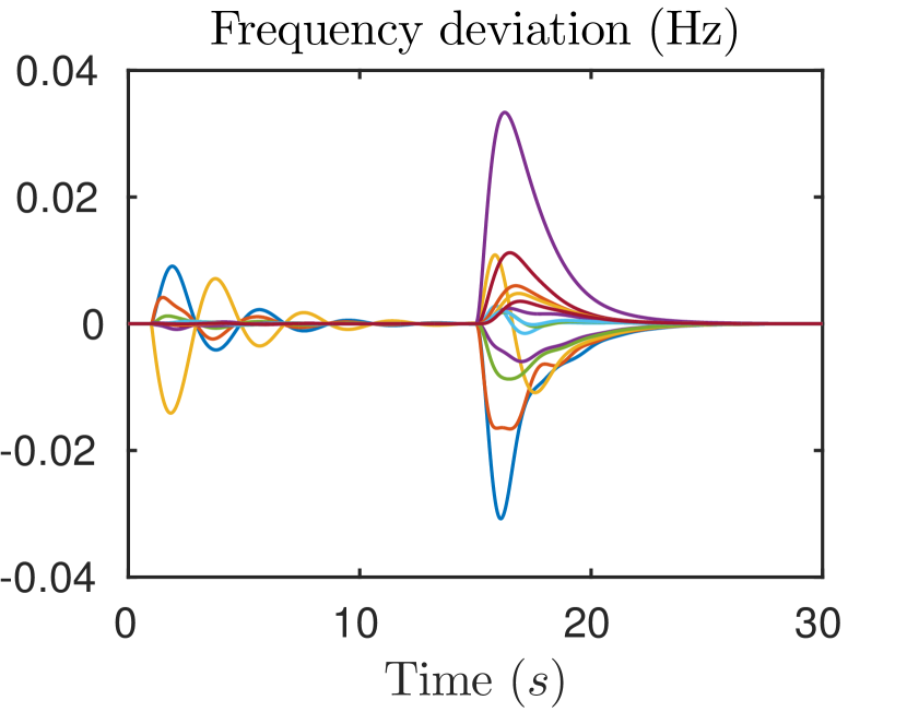
(a) Evolution of the frequency deviation. After each change of the load or the cost functions, the frequency is restored to its nominal value.

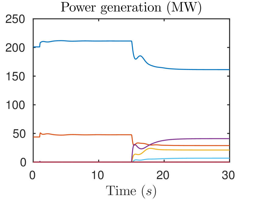
(b) Evolution of the power generation at each node. After the change of the cost functions in nodes $3,6,8$, there is more competition among the generators, resulting in lower power productions at node $1$ and $2$.

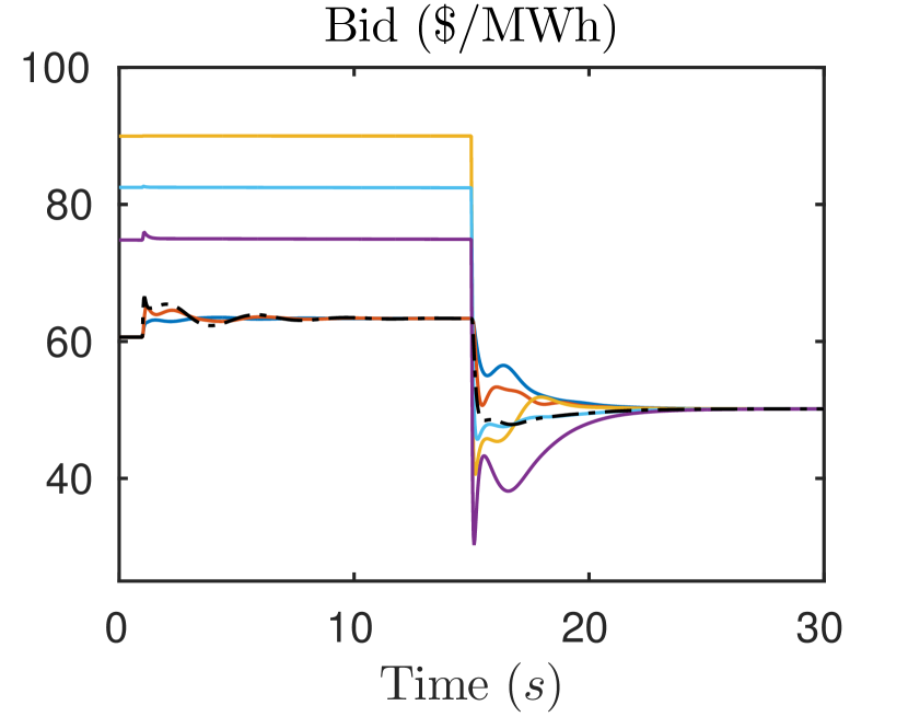
(c) Evolution of the bids and the Lagrange multiplier (represented by the dashed black colored line). Initially, the marginal costs (and the bids) at zero power production are higher than the market equilibrium price for nodes $3,6,8$.

Figure 2: Simulations of the interconnection (13) between the ISO-generation bidding mechanism and the power network dynamics with $\sigma=300$. At $t=$1\text{\,}\mathrm{s}$$ the load at node $3$ is increased from $80\text{\,}\mathrm{MW}$ to $94.2\text{\,}\mathrm{MW}$. At $t=$15\text{\,}\mathrm{s}$$ the marginal cost decreases at nodes $3,6,8$ which allows these generators to make profit by lowering their bids to have a positive power production as illustrated in plots (b) and (c).

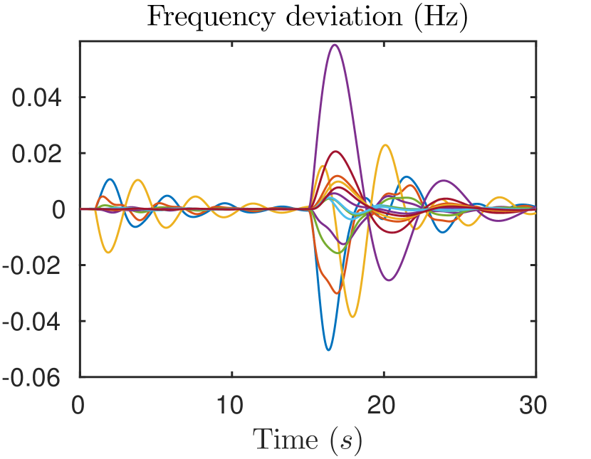
(a) Evolution of the frequency deviation. Compared to Figure 2(a), there are more oscillations and a larger overshoot of the frequency deviations.

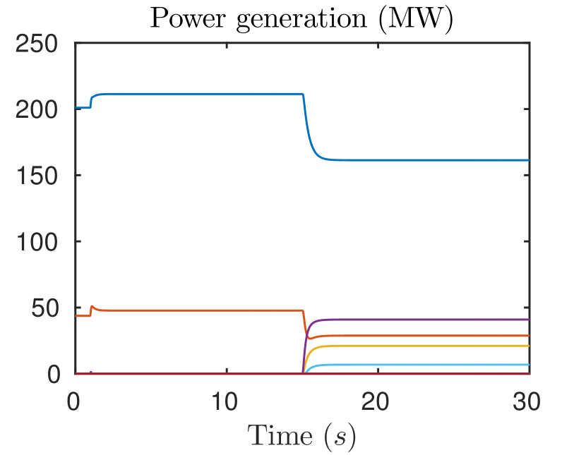
(b) Evolution of the power generations at each node. As $\sigma=0$, the generations are updated only according to the bidding process without using any frequency measurements.

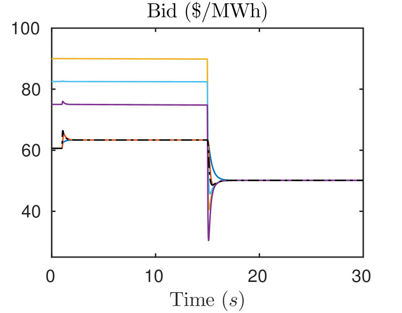
(c) Evolution of the bids and the Lagrange multiplier. Compared to Figure 2(c), the convergence is faster in this scenario because the bidding process does not take into account its impact on the dynamics of the power network.

Figure 3: Simulations of the interconnection (13) between the ISO-generation bidding mechanism and the power network dynamics for the case of $\sigma=0$, i.e., when there is no frequency feedback signal in the bidding process. The scenario is the same as in Figure 2. As illustrated, the closed-loop system also converges in this case to an efficient equilibrium.

At $t=$15\text{\,}\mathrm{s}$$ the cost of producing electricity is decreased in areas $3,6,8$ by setting $(q_{3},q_{6},q_{8})=(60,75,68)$ and $(c_{3},c_{6},c_{8})=(38,45,23)$. This allows these generators to make profit by participating in the bidding process and results in a reduction of the total cost of the generation from $9711\text{\,}\$\mathrm{/}\mathrm{h}$ to $8540\text{\,}\$\mathrm{/}\mathrm{h}$. As illustrated in both Figures 2 and 3, the power generations converge to the new optimal steady state given by

$$(P_{g1},P_{g2},P_{g3},P_{g6},P_{g8})=(161,29,21,7,41).$$

In addition, we observe that after each change of either the load or the cost function, the frequency is stabilized and the bids converge to a new efficient Nash equilibrium. The fact that the frequency transients are better in Figure 2 than in Figure 3 is consistent, since in the latter case there is no frequency feedback in the bidding process.

VII Conclusions

We have studied a market-based power dispatch scheme and its interconnection with the swing dynamic of the physical network. From the market perspective, we have considered a continuous-time bidding scheme that describes the negotiation process between the independent system operator and a group of competitive generators. Using the frequency as a feedback signal in the bidding dynamics, we have shown that the interconnected projected dynamical system provably converges to an efficient Nash equilibrium (where generation levels minimize the total cost) and to zero frequency deviation. In this way, competitive generators are enabled to participate in the real-time electricity market without compromising efficiency and stability of the power system. Future work will investigate finite-horizon scenarios and incorporate generator bounds and power flow constraints in the economic dispatch formulation.

Theorem .1 (Invariance principle for complementarity systems [18]).

Consider the system

$$\dot{x} =F(x)+C^{T}\Lambda$$ (23a)

$$0 \leq Cx+d\perp\Lambda\geq 0$$ (23b)

with Lipschitz continuous $F$ and let $K$ be the polyhedron

$$K=\{x:Cx+d\geq 0\}.$$ (24)

Let $\Psi\subset{}^{n}$ be a compact set and $V:{}^{n}\rightarrow\real$ be a continuous differentiable function such that

Let $E\subset\mathbb{R}^{n}$ be given by

$$E:=\{x\in K\cap\Psi:\langle F(x),\nabla V(x)\rangle=0\}$$

and denote the largest invariant subset of $E$ by $\mathcal{M}$. Then, for each $x_{0}\in K$ such that its orbit satisfies $\gamma(x_{0})\subset\Psi$, we have

$$\lim_{t\to\infty}d(x(t;t_{0},x_{0}),\mathcal{M})=0.$$

References

• [1] T. Stegink, A. Cherukuri, C. D. Persis, A. van der Schaft, and J. Cortés, “Stable interconnection of continuous-time price-bidding mechanisms with power network dynamics,” in Power Systems Computation Conference, Dublin, Ireland, 2018, submitted.
• [2] S. Trip, M. Bürger, and C. De Persis, “An internal model approach to (optimal) frequency regulation in power grids with time-varying voltages,” Automatica, vol. 64, pp. 240–253, 2016.
• [3] X. Zhang and A. Papachristodoulou, “A real-time control framework for smart power networks: Design methodology and stability,” Automatica, vol. 58, pp. 43–50, 2015.
• [4] N. Li, C. Zhao, and L. Chen, “Connecting automatic generation control and economic dispatch from an optimization view,” IEEE Transactions on Control of Network Systems, vol. 3, no. 3, pp. 254–264, 2016.
• [5] S. T. Cady, A. D. Domínguez-García, and C. N. Hadjicostis, “A distributed generation control architecture for islanded AC microgrids,” IEEE Transactions on Control Systems Technology, vol. 23, no. 5, pp. 1717–1735, 2015.
• [6] F. Dörfler, J. W. Simpson-Porco, and F. Bullo, “Breaking the hierarchy: Distributed control and economic optimality in microgrids,” IEEE Transactions on Control of Network Systems, vol. 3, no. 3, pp. 241–253, 2016.
• [7] F. Alvarado, J. Meng, C. DeMarco, and W. Mota, “Stability analysis of interconnected power systems coupled with market dynamics,” IEEE Transactions on Power Systems, vol. 16, no. 4, pp. 695–701, 2001.
• [8] D. J. Shiltz, M. Cvetković, and A. M. Annaswamy, “An integrated dynamic market mechanism for real-time markets and frequency regulation,” IEEE Transactions on Sustainable Energy, vol. 7, no. 2, pp. 875–885, 2016.
• [9] T. Stegink, C. De Persis, and A. van der Schaft, “A unifying energy-based approach to stability of power grids with market dynamics,” IEEE Transactions on Automatic Control, vol. 62, no. 6, pp. 2612–2622, 2017.
• [10] A. Cherukuri and J. Cortés, “Iterative bidding in electricity markets: rationality and robustness,” arXiv preprint arXiv:1702.06505, 2017, submitted to IEEE Transactions on Control of Network Systems.
• [11] ——, “Decentralized Nash equilibrium learning by strategic generators for economic dispatch,” in American Control Conference (ACC), 2016.   IEEE, 2016, pp. 1082–1087.
• [12] J. Machowski, J. Bialek, and J. Bumby, Power System Dynamics: Stability and Control, 2nd ed.   Ltd: John Wiley & Sons, 2008.
• [13] T. Başar and G. Oldser, Dynamic Noncooperative Game Theory.   Academic Press, 1982.
• [14] D. Fudenberg and J. Tirole, Game Theory.   Cambridge, MA: MIT Press, 1991.
• [15] J.-B. Hiriart-Urruty and C. Lemaréchal, Convex analysis and minimization algorithms I: Fundamentals.   Springer science & business media, 2013, vol. 305.
• [16] A. Cherukuri, B. Gharesifard, and J. Cortes, “Saddle-point dynamics: conditions for asymptotic stability of saddle points,” SIAM Journal on Control and Optimization, vol. 55, no. 1, pp. 486–511, 2017.
• [17] R. Goebel, “Stability and robustness for saddle-point dynamics through monotone mappings,” Systems & Control Letters, vol. 108, pp. 16–22, 2017.
• [18] B. Brogliato and D. Goeleven, “The Krakovskii-LaSalle invariance principle for a class of unilateral dynamical systems,” Mathematics of Control, Signals and Systems, vol. 17, no. 1, pp. 57–76, 2005.
• [19] B. Brogliato, A. Daniilidis, C. Lemaréchal, and V. Acary, “On the equivalence between complementarity systems, projected systems and differential inclusions,” Systems & Control Letters, vol. 55, no. 1, pp. 45–51, 2006.