Hysteresis in the Ising model with Glauber dynamics.

Abstract

We use Glauber dynamics to study time and temperature dependence of hysteresis in the pure (without quenched disorder) Ising model on cubic, square, honeycomb lattices as well as random graphs. Results are discussed in the context of more extensive studies of hysteresis in the random field Ising model.

I introduction

The purpose of this note is to report work on temperature-driven hysteresis  bertotti in pure (i.e. without quenched disorder) Ising model  ising ; onsager and compare it with more extensively studied case of disorder-driven hysteresis in the zero-temperature ($T=0$) random field Ising model (ZTRFIM) sethna1 ; maritan ; sethna2 ; dhar ; sethna3 ; perez ; sethna4 ; xavier ; rosinberg ; liu ; spasojevic ; balog ; shukla . Hysteresis in ZTRFIM has been studied largely, if not entirely, in the limit of driving frequency $\omega\to 0$. Normally hysteresis should vanish as $\omega\to 0$, but it survives because the limit $T\to 0$ is taken before the limit $\omega\to 0$. This is implemented by using $T=0$ Glauber dynamics  glauber to update spins, and holding the applied field $h$ constant during updates. Thus one starts with all spins down in a sufficiently large and negative $h$, increases $h$ slowly till one spin flips up and causes a connected cluster of spins surrounding it to flip up in an avalanche. When the avalanche stops, $h$ is increased again until another avalanche occurs. The entire hysteresis loop is determined in this way by changing $h$ minimally between avalanches but keeping it fixed during avalanches.The dynamics of ferromagnetic ZTRFIM is Abelian. The order in which unstable spins are flipped does not matter. The stable configuration at $h$ is the same whether we reach it through a series of avalanches as described above or in one big avalanche starting from an initial state with all spins down.

A common choice for the random field distribution is a Gaussian with average zero and standard deviation $\sigma$. On simple cubic and several other lattices, there exists a critical value of $\sigma=\sigma_{c}$ that marks a phase transition in the response of the system to the applied field. For $\sigma>\sigma_{c}$ the magnetization $m(h)$ is smooth function of $h$, but for $\sigma<\sigma_{c}$ it acquires discontinuities at $h=\pm h_{c}$. The discontinuities reduce in size with increasing $\sigma$ and vanish continuously as $\sigma\to\sigma_{c}$. Extensive numerical and analytic work has established scale invariance and universality of phenomena in the vicinity of the non-equilibrium critical points $\{\pm h_{c},\sigma_{c}\}$ in close parallel to the equilibrium critical behavior seen in the pure Ising model near the critical temperature $T_{c}$  wilson . Indeed the parameter $\sigma$ in the ZTRFIM plays a role analogous to temperature $T$ in the pure Ising model. Although this similarity is well known, to the best of our knowledge, it has not been tested directly by simulating the $\omega$-dependent hysteresis loops in pure Ising model on a regular lattice.

We consider the kinetic Ising model on a cubic lattice characterized by the Hamiltonian,

$$H=-J\sum_{i,j}s_{i}s_{j}-h\sum_{i}s_{i}$$

Here $J$ is ferromagnetic interaction between nearest neighbor Ising spins $\{s_{i}=\pm 1\}$ situated on sites $\{i=1,2,\ldots,N\}$, and $h$ is a uniform applied field measured in units of $J$. We assume the system is in contact with a heat reservoir at temperature $T$. The Glauber prescription for updating a configuration $\{s_{i}\}$ is: (i) choose a site at random, say site $i$, (ii) calculate the local energy at site $i$, $e_{i}=-J\sum_{j\neq i}s_{j}-h$, (iii) flip $s_{i}$ to $-s_{i}$ with probability $1/(1+exp(-2Ke_{i}))$, where $K=J/k_{B}T$ and $k_{B}$ is the Boltzmann constant, (iv) repeat the above procedure $N$ times to complete one Monte Carlo cycle (unit of time), and (v) continue for $t$ Monte Carlo cycles. The above dynamics has two important properties; detailed balance and ergodicity. These properties combine to thermalize the system with increasing $t$. The dynamics of a fully thermalized system in the limit $t\to\infty$ generates configurations which are distributed according to their respective Boltzmann weights and are therefore uncorrelated with the initial configuration $\{s_{i}\}$ at $t=0$. The time average of a thermodynamic quantity over a sufficiently large number of such configurations should approximate to the corresponding equilibrium value obtained from the partition function of the system. An exact calculation of partition function is generally not feasible, so Glauber’s or some other similar dynamics is the only practical way to explore equilibrium behavior of a system. However, predicting equilibrium behavior from dynamics has its own difficulties. Numerical studies are necessarily restricted to finite $t$ while equilibrium properties correspond to $t\to\infty$. It is not easy to decide what value of $t$ is adequate to extrapolate the results to equilibrium behavior. The answer depends on the temperature of the system and whether it is above or below the critical temperature. Our interest in the present paper is primarily in hysteresis which is a non-equilibrium phenomenon seen at finite $t$ only. We will examine how hysteresis decreases with increasing $t$ and if this behavior is consistent with the equilibrium behavior of the system reported in the literature. The equilibrium magnetization per site $m(h)=\sum_{i}s_{i}/N$ depends on $K$. There is a critical value $K_{c}=0.22165435(45)$ on a simple cubic lattice which marks the onset of spontaneous symmetry breaking in the system  binder ; sonsin ; preis ; gupta ; haggkvist . In the limit $t\to\infty$, at $h=0$, $m(h=0)\to 0$ if $K<K_{c}$, but $m(h=0)\to\pm m^{*}(K)$ with equal probability if $K\geq K_{c}$, where $|m^{*}(K)|$ increases continuously from zero to unity as $K$ increases from $K=K_{c}$ to $K=\infty$.

Hysteresis is generally characterized by a system’s response to a cyclic field, but we may also consider it as a measure of system’s memory of its initial state for $t<\infty$. It has been studied in several ways depending upon how the cyclic field is ramped up and down rao ; samoza ; thomas ; zheng . We choose a method close in spirit to the one used in the ZTRFIM. We fix $K$ and $h$, and evolve two initial states $\{s_{i}=-1\}$ and $\{s_{i}=1\}$ separately for time $t$. Initially, the two states have magnetization per site equal to $-1$ and $+1$ respectively. Let the corresponding values at time $t$ be $m_{-}(K,h,t)$ and $m_{+}(K,h,t)$. Our simulations show that $m_{+}(K,h,t)>m_{-}(K,h,t)$ and the difference $m_{+}(K,h,t)-m_{-}(K,h,t)$ decreases with increasing $t$. This is to be expected from the properties of dynamics mentioned earlier. As the system approaches thermalization, the output configurations of the dynamics become uncorrelated with the initial configurations. Hysteresis becomes negligible at very large negative or positive values of $h$ $(|h|>>J)$ even for relatively small $t$ because the probability that a spin remains aligned opposite to a very large field is exponentially small. Thus, if $|h|>>J$, $m_{-}(K,h,t)\approx m_{+}(K,h,t)\approx\operatorname{sgn}h$.

II Numerical Results

In our simulations, we choose a large range of $h$ around $h=0$, $[-H_{0},H_{0}]$, such that induced magnetizations at $\pm H_{0}$ are nearly $\pm 1$. We divide the interval $[-H_{0},H_{0}]$ into $n$ equal parts of width $\delta h=2H_{0}/n$, and calculate $m_{-}(K,h,t)$ and $m_{+}(K,h,t)$ at each increment $h_{i}=-H_{0}+i\times\delta h;i=0,\ldots,n$. We choose $n$ to be reasonably large so that the locus of data points on the graph indicates the shape of a continuous curve in the limit $n\to\infty$. We may call this curve the hysteresis loop at characteristic time period $t$ because each point on the curve has evolved for a time $t$ under the relaxation dynamics. The results are shown in Fig.1 for three values of $K$ in the vicinity of $K_{c}$ and two values of $t$ for each $K$. An interesting feature of Fig.1 is that the curves for $m_{-}(K,h,t)$ and $m_{+}(K,h,t)$ move towards each other as $t$ increases and look qualitatively similar to the hysteresis loops produced by a driving field of the form $h(t)=-H_{0}\cos{\omega t}$, or a field that is ramped up and down in the form $h(t)=-H_{0}+\omega t$ and $h(t)=H_{0}-\omega t$ respectively. Here $\omega=\Delta h/\Delta t$, and relaxation dynamics is applied to a configuration $\{s_{i}\}$ for a time $\Delta t$ at $h$ and the output is used as input at $h+\omega\Delta t$. The fact that different methods produce similar hysteresis loops suggests that the generic $s$-shape of hysteresis loops comes from the probability distribution used in the relaxation dynamics rather than the form of the driving field. Notwithstanding the similarity of hysteresis loops, detailed behavior does depend on how the applied field is varied. A detail that interests us particularly is the variation of coercive field $H_{c}$ with $t$ for a given $K$. Fig.1 indicates the trend that $H_{c}$ moves towards $h=0$ with increasing $t$. More detailed study requires monitoring the system at each value of $t$ and much smaller increments $\delta h$ in the applied field $h$ in the vicinity of $H_{c}$. This increases the computation time enormously and a compromise has to be made with respect to the size of $\delta h$. We have used $\delta h=0.001$ for cubic lattice and $\delta h=0.01$ for other lattices. This means that coercive fields in the range $0<H_{c}\leq\delta h$ will be clubbed at $H_{c}=\delta h$ in the respective cases. We will return to this point when discussing Fig.2, Fig.3, and Fig.4.

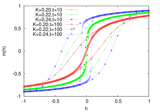
Figure 1: Six hysteresis loops ($K=0.20,0.22,0.24;t=10,100$ for each $K$) for pure Ising model on a $50^{3}$ cubic lattice near $K_{c}\approx 0.221654$. The figure suggests that hysteresis vanishes as $t\to\infty$ but it vanishes differently for $K<K_{c}$ than for $K>K_{c}$. For $K=0.20,t=100$, hysteresis has already vanished on the scale of the figure and $m(h)$ is continuous at $h=0$. For $K=0.24$, hysteresis at $t=100$ has reduced from its value at $t=10$ and $m(h)$ curves have come closer to vertical near the coercive field $H_{c}$. In this case, hysteresis is expected to vanish as $t\to\infty$ accompanied by a discontinuity in $m(h)$ at $h=0$.

Fig.1 shows hysteresis loops for $N=50^{3}$, $K=0.20,0.22$, $0.24$, $t=10$, and $100$. It reveals two features of general validity. Firstly, hysteresis decreases with increasing $t$. For each $K$, the loop shrinks as we go from $t=10$ to $t=100$. The shrinking is faster if $K<K_{c}$ and the rate of shrinking increases with increasing $K_{c}-K$. At $t=100$ the loop is hardly visible for $K=0.22$ and not at all for $K=0.20$ on the scale of the figure. Secondly, the shape of loop changes with increasing $t$. It changes differently for $K<K_{c}$ than for $K>K_{c}$. If $K<K_{c}$, the loop tends to become narrower and elongated along the $x$-axis with increasing $t$. Eventually the loop collapses into a single continuous curve that passes through the origin $h=0$. If $K>K_{c}$, the loop becomes narrower and elongated along the $y$-axis with increasing $t$. In this case the middle portion of the $s$-shaped magnetization curve $m(h)$ becomes nearly vertical at the coercive field $H_{c}$ which moves very slowly towards $h=0$ with increasing $t$. In simulations, fluctuations make it rather difficult to distinguish between a continuous but steep change in $m(h)$ from a discontinuity in $m(h)$. We have checked this point carefully and conclude there is no discontinuity in $m(h)$ for finite $t$ up to the largest $t$ that we could test. In case there appeared to be a discontinuity in $m(h)$ at $H_{c}$, we re-examined the neighborhood of $H_{c}$ more closely by increasing the system size and decreasing the spacing $\delta h$ between neighboring $h$ values in the vicinity of $H_{c}$. This generated new data points inside the apparent discontinuity and indicated a sharply rising but continuous $m(h)$. We may also add that there is no theoretical reason to expect a true discontinuity in $m(h)$ at any finite $t$ for $T>0$. This suggests an approximate picture of the hysteresis loop as a flagpole with one dimensional flags at both ends but in opposite directions. The length of the flagpole increases with increasing $K-K_{c}$ and its width decreases with increasing $t$. As $t\to\infty$, we may expect the two halves of the loop to collapse on top of each other and the flagpole replaced by a discontinuity in $m(h)$ at $h=0$.

The above discussion suggests that the manner in which hysteresis decreases with increasing $t$ can reveal if the system is above or below its critical point. One can either monitor the rate at which the area of the hysteresis loop decreases, or alternately, how the coercive field decreases with increasing $t$. Fig.2 shows $H_{c}$ vs. $t$ on the lower half of the hysteresis loop for $N=50^{3}$, $K=0.10,0.20,0.22,0.221654,0.24,1.00$, $1\leq t\leq 2048$, and $0.001\leq H_{c}\leq 4$. We have used logarithmic binning to reduce fluctuations in the data at large $t$ and drawn a line $H_{c}=1/t$ for comparison. It takes a good deal of computer time (several days) to generate the data shown in Fig.2 and it is the best we can do within our resources. So we look closely for possible trends in the data even if these trends are not as clear as we would desire. We see that four graphs corresponding to $K\leq K_{c}$ are closer to each other and different from two graphs for $K>K_{c}$. If $K<<K_{c}$, thermal fluctuations are very large and consequently the equilibrium correlation length is very short. Therefore the system relaxes to a thermalized state in a short time. As $K\to K_{c}$, the correlation length increases and so does the time to thermalization. Eventually at $K=K_{c}$ the correlation length and the time to thermalization diverge algebraically. At a given $t$, we may consider the magnitude of coercive field $H_{c}$ as a measure of the distance from equilibrium. Therefore we may expect $H_{c}$ to vary with $t$ as a power law at $K=K_{c}$. Our data indicates $H_{c}\sim t^{-1.15}$ approximately over two decades of $t$. Graphs for $K<K_{c}$ appear to behave similarly after an initial transient period and before fluctuations blur the trend. In the limit $K\to 0$ and $t\to\infty$, the spins would tend to flip independently of each other. System of $N=50^{3}$ will have random fluctuation in $m(h)$ of the order of $N^{-1/2}\approx 0.003$ around the value $m(H_{c})=0$. The coercive field required to reverse the magnetization will have similar fluctuations. This is the reason why $H_{c}$ for $K=0.10$ shows a plateau at $H_{c}\approx 0.003$ and $t>512$. Similarly in the case of $K=0.22$ and $K=0.22165$, plateaus are seen at $H_{c}\approx 0.002$ at $t>1024$. A plateau in $H_{c}$ at large $t$ could be expected for $K=0.20$ as well but its absence is within expected fluctuations. Next we turn our attention to graphs for $K>K_{c}$.In this regime thermal fluctuations diminish and long range order develops through nucleation, growth, coarsening of domains, and magnetization reversal. These processes are exceedingly slow due to smallness of thermal excitations. A large fraction of Glauber moves fail to flip the spins thus retarding the evolution of the system. Consequently $H_{c}$ decreases more slowly with increasing $t$ if $K>K_{c}$ than it does if $K<K_{c}$. The equilibrium value of order parameter increases with increasing $K$. Thus a magnetization reversal curve from a metastable state to a stable state at $H_{c}$ takes a nearly vertical shape in the vicinity of $H_{c}$ if $K>>K_{c}$. It takes a long time for relaxation dynamics to reverse the magnetization. A droplet of up spins has to nucleate in a sea of down spins and slowly grow to the system size. This is a very slow process and becomes progressively slower as $K$ increases. In the range of $t=1$ to $2024$, $H_{c}$ drops from $3.03$ to $0.05$ if $K=0.24$ and $3.47$ to $1.83$ if $K=1.00$. There is no good evidence that $H_{c}$ decreases with $t$ as a power law, nor we know of any theoretical reason to expect so. However, we note for later discussion that this very slow decrease of $H_{c}$ with $t$ for $K>K_{c}$ is a signature of a discontinuity in $m(h)$ at $h=0$ in the limit $t\to\infty$. The point is that for $K>K_{c}$ equilibrium $m(h)$ vs. $h$ curve must have a discontinuity at $h=0$ on grounds of symmetry breaking but it is difficult to observe the sharpness of this discontinuity via hysteresis dynamics in the limit $t\to\infty$. To the best of our knowledge, the limit $t\to\infty$ for this purpose has not been accessed even with the best of computers and most efficient Monte Carlo codes particularly for $K>>K_{c}$. The relaxation of the system is just too slow to reach equilibrium on practical time scales for $K>>K_{c}$. Quite often the sharpness of a first order transition is replaced by hysteresis in simulations as well as laboratory experiments. Thus we have to be content with the signature indicated above for the interpretation of our results in this regime.

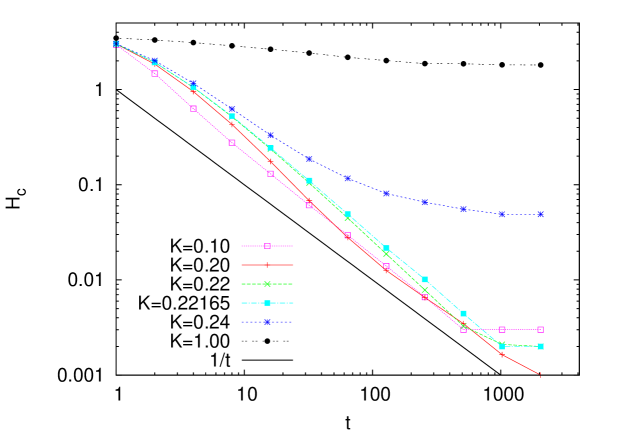
Figure 2: Coercive field $H_{c}$ on lower half of hysteresis loop after $t$ Monte Carlo cycles of Glauber dynamics on a $50^{3}$ cubic lattice starting with all spins down. A line $H_{c}=1/t$ is drawn for reference. If $K<K_{c}$, $H_{c}$ vanishes rapidly as $t\to\infty$. If $K>K_{c}$, $H_{c}$ decreases more and more slowly as $K$ increases. The reason is that $m(h)$ curve near $H_{c}$ tends to become vertical and it takes much longer time to reverse magnetization at $H_{c}$. It is a signature that $m(h)$ may acquire a discontinuity at $h=0$ in the limit $t\to\infty$ if $K>K_{c}$.

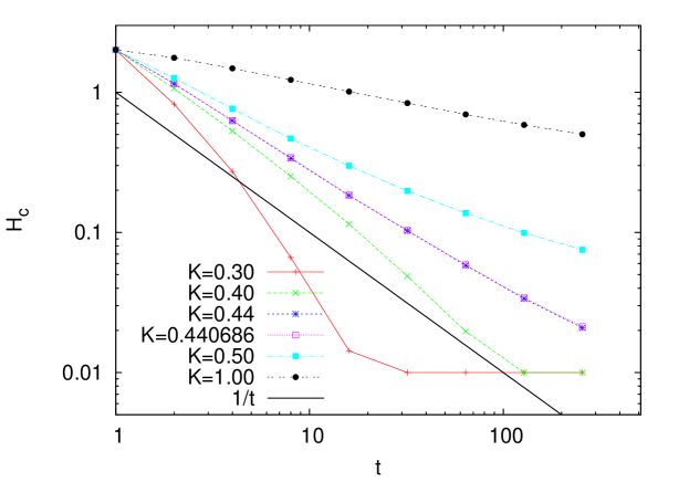
Figure 3: Coercive field $H_{c}$ on a $500\times 500$ square lattice for different values of $K$ and time periods $t$. The qualitative behavior on the square lattice is the same as on the cubic lattice. It indicates that $m(h)$ curve may acquire a discontinuity at $h=0$ in the limit $t\to\infty$ if $K>K_{c}$. A plateau is seen at $H_{c}=0.01$ because the system was monitored at increments of applied field equal to $0.01$.

We have also studied hysteresis and the variation of $H_{c}$ with $t$ on square and honeycomb lattices on the above lines. Ising models on these lattices are known to undergo equilibrium phase transitions at $K_{c}\approx 0.440686$ and $K_{c}=0.658479$ respectively. The exact values are given by $\sinh{2K_{c}}=1$  onsager and $\cosh{2K_{c}}=2$  wannier . $H_{c}$ vs. $t$ graphs for the two cases are presented in Fig.3 and Fig.4 for lattices of size $500^{2}$, $1\leq t\leq 512$, and $0.01\leq H_{c}\leq 3$. Fig.3 shows the behavior on a square lattice for $K=0.30,0.40,0.44,0.440686,0.50,1.00$. A line $H_{c}=1/t$ has been drawn for comparison. Graphs for $K=0.44$ and $K=0.440686$ are indistinguishable on the scale of figure and both vary approximately as $H_{c}\sim t^{-0.85}$. Graphs for $K=0.40$ and $K=0.30$ decay more rapidly but there is no discernible power law associated with the decrease. Two values of $K>K_{c}$, $K=0.50,1.00$, indicate that $m(h)$ may hit a discontinuity at $h=0$ as $t\to\infty$ consistent with the known equilibrium phase transition in the system. We may add that an argument similar to the one used to explain the plateau in Fig.2 at $H_{c}\approx 0.003$ would lead us to expect plateaus in Fig.3 and Fig.4 around $H_{c}\approx N^{-1/2}=0.002$ for large $t$ and $K<<K_{c}$. But these are pre-empted by a larger step size $\delta h=0.01$ used in generating the data on square and honeycomb lattices. On these lattices, coercive fields in the range $0<H_{c}\leq 0.01$ are binned together resulting in a plateau at $H_{c}=0.01$. Because the plateau is an order of magnitude higher in comparison with Fig.2, time periods required to hit the plateau are smaller by an order of magnitude. This reduces the computer time without seriously compromising the general trends implicit in the data. In short, the behavior on the square lattice appears qualitatively similar to the behavior on the cubic lattice. Earlier we alluded to differences in hysteresis depending upon different forms of the driving field. Differences between sinusoidal and linear driving fields have been noted in the literature  rao ; samoza ; thomas ; zheng . Fig.2 and Fig.3 provide another example. They indicate $H_{c}\sim t^{-1.15}$ on cubic, and $H_{c}\sim t^{-0.85}$ on square lattice at $K=K_{c}$. A subtle point to note is that the power-law fit on the square lattice is not quite as good as it is on the cubic lattice. A close look at Fig.3 shows that the critical curve turns up slightly at larger values of $t$. A possible explanation may be that $K_{c}$ on square lattice is obtained from the exact solution of the partition function while $K_{c}$ on cubic lattice is obtained from Glauber dynamics. It maybe that critical values of $K_{c}$ obtained from the two methods are somewhat different. This notwithstanding we can compare our power-laws with those for a field which is swept up from $-H_{0}$ to $H_{0}$ and back to $H_{0}$ in $t$ steps and at each step the previous output is used as the new input to dynamics. In this case, results for the area $A_{c}$ of the hysteresis loop at $K_{c}$ are available zheng . There is no exact relationship between $H_{c}$ and $A_{c}$ but they should be approximately proportional to each other in the limit $t\to\infty$. The reported results are $A_{c}\sim t^{-0.495}$ on cubic and $A_{c}\sim t^{-0.408}$ on square lattice which are significantly different from the power-laws observed in our version of the dynamics. We find hysteresis on honeycomb lattice to be qualitatively similar to that on cubic and square lattices. Fig.4 shows $H_{c}$ vs $t$ at $K_{c}=0.658479$, two values of $K<K_{c}$ and one value of $K>K_{c}$. The graphs for $K=K_{c}$ and $K>K_{c}$ show similar trend; both seem to be headed for an ordered state. This means that effective $K_{c}$ seen by dynamics is smaller than $K_{c}=0.658479$. The difference between $K_{c}$ and effective $K_{c}$ is larger on honeycomb lattice as compared with the same on square lattice.

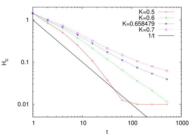
Figure 4: Coercive field $H_{c}$ vs. $t$ on a $500\times 500$ honeycomb lattice at different time periods $t$ for $K=0.5,0.6,0.658479,0.7$. The figure indicates that effective transition point seen by the dynamics is smaller than $K_{c}=0.658479$.

In order to reconfirm and verify the trends indicated above, we have examined remanent magnetization $m_{R}$ on the lower half of hysteresis loop as a function of $t$; $m_{R}$ is the magnetization per site at $h=0$ starting from the initial state with all spins down. Time dependence of $m_{R}$ is relatively easy to monitor and it is a good indicator whether the system is evolving towards a disordered or an ordered state. If $K\leq K_{c}$, we expect $m_{R}$ to decrease to zero with increasing $t$. This is born out by the results shown in Fig.5, Fig.6, Fig.7, and Fig.8. These figures show $m_{R}$ vs. $t$ on cubic, square, and honeycomb lattices, as well as on a random graph of coordination number $z=3$. Some noteworthy features are as follows. Irrespective of the lattice type, if $K<<K_{c}$, correlation lengths are very short and $m_{R}$ approaches zero with increasing $t$ as expected. Consider Fig.5 for cubic lattice. At $K=K_{c}$, $m_{R}$ increases more slowly towards zero and somewhat surprisingly overshoots it at $t\approx 5000$. Such magnetization reversals are allowed within large critical fluctuations at $K=K_{c}$ but these should average out to zero eventually because the equilibrium value of the order parameter is zero. For $K>K_{c}$, we may expect $m_{R}$ to approach a finite value with increasing $t$ as indeed is seen in the Fig.5 for the cubic lattice. Fig.6 for square lattice shows similar behavior except for the case $K=K_{c}$ where there is some indication that $m_{R}$ may perhaps level off at a finite value for larger times. As mentioned earlier in reference to Fig.3, this may indicate that the effective $K_{c}$ for single-spin-flip Glauber dynamics may be somewhat smaller than $K_{c}=0.440686$. Fig.7 indicates similar behavior on honeycomb lattice. The effective $K_{c}$ recognized by dynamics on honeycomb lattice is apparently much smaller than $K_{c}=0.658479$. These results are consistent with the results shown in Fig.3 and Fig.4 and our interpretations of those figures. For reason to be discussed below we also examined $m_{R}$ on a random graph with coordination number $z=3$ which is a good representation of a Bethe lattice of the same connectivity. The exact $K_{c}$ on the Bethe lattice is given by the equation $\tanh{K_{c}}=(z-1)^{-1}$  rozikov . The case $z=2$ corresponds to one dimensional Ising model which does not have a phase transition to an ordered state at any finite $K_{c}$. Thus, under the Glauber dynamics, remanent magnetization $m_{R}$ for $z=2$ should approach zero irrespective of $K$. We have verified that this is indeed the case. Of course, starting with all spins down, the time $t$ taken to thermalize increases with increasing $K$. For $z=3$, we have $K_{c}=0.54930615$ approximately. Remanence magnetization on corresponding random graph is shown in Fig.8. It indicates the occurrence of a phase transition in the system unlike the corresponding case in ZTRFIM. There is clear evidence that Glauber dynamics takes the system to an ordered state on a random graph of connectivity $z=3$ if $K>K_{c}$.

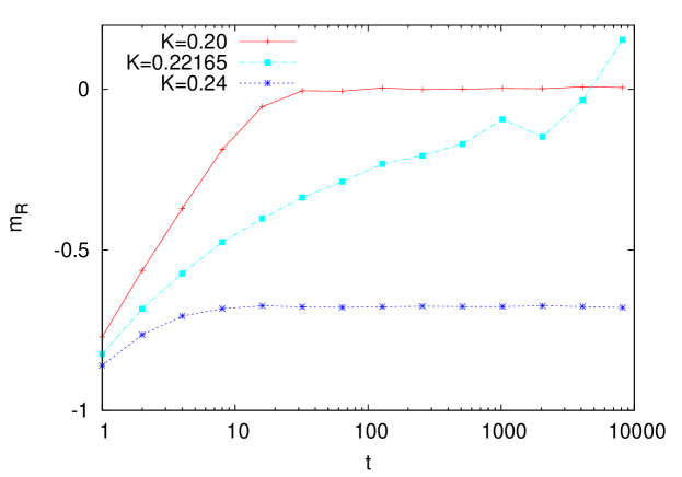
Figure 5: Remanent magnetization $m_{R}$ vs. $t$ on a $100^{3}$ cubic lattice on the lower half of the hysteresis loop for three representative values of $K$. As $t$ increases $m_{R}$ increases towards its equilibrium value; zero if $K\leq K_{c}$, and a finite value if $K>K_{c}$. Magnetization reversal at $t\approx 5000$ for $K=K_{c}$ is a result of large critical fluctuations.

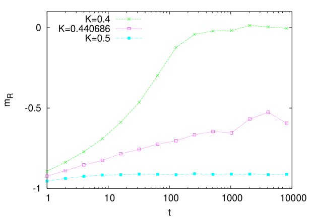
Figure 6: Remanence $m_{R}$ vs. $t$ on a $500\times 500$ square lattice for three representative values of $K$. As $t$ increases $m_{R}$ is seen to approach its equilibrium value; zero if $K<K_{c}$ and a finite value if $K>K_{c}$. The limiting behavior for $K=K_{c}$ is not very clear. If $m_{R}$ eventually levels off at a finite value, it would indicate that the Onsager $K_{c}=0.440686$ is somewhat higher than appropriate $K_{c}$ for single-spin-flip Glauber dynamics.

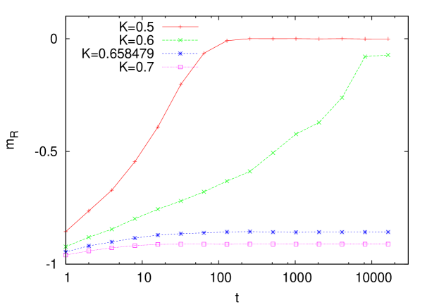
Figure 7: Remanence $m_{R}$ vs. $t$ on a $500\times 500$ honeycomb lattice obtained from Glauber dynamics for four representative values of $K$. The critical value $K_{c}=0.658479$ is obtained from partition function; $m_{R}$ is expected to approach zero if $K\leq K_{c}$, and a finite value if $K>K_{c}$. The plateau at $K_{c}$ suggests that the dynamical transition to an ordered state occurs at a higher temperature than predicted by the partition function.

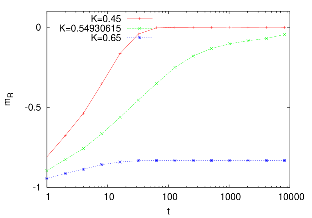
Figure 8: Remanence $m_{R}$ vs. $t$ on a random graph $(z=3,N=10^{6})$ obtained from single-spin-flip Glauber dynamics. The critical value $K_{c}=0.54930615$ is obtained from partition function; $m_{R}$ is expected to approach zero if $K\leq K_{c}$, and a finite value if $K>K_{c}$. The figure indicates a phase transition on a $z=3$ random graph unlike the case in ZTRFIM.

III Discussion

As mentioned in the Introduction, primary motivation for our study came from the curious similarity between nonequilibrium critical phenomena in ZTRFIM in the vicinity of $\sigma_{c}$ and equilibrium critical phenomena in pure Ising model in the vicinity of $K_{c}$. Does the similarity between $\sigma$ and $K$ hold only at the respective critical points or is it more extended? What would an extended similarity mean? We can not extract equilibrium behavior from hysteresis in ZTRFIM but we can explore equilibrium as well as nonequilibrium behavior of pure Ising model by supplementing it with finite temperature Glauber dynamics. The obvious thing is to compare phases on both sides of $\sigma_{c}$ with phases on both sides of $K_{c}$ and extend equilibrium studies in pure Ising model to nonequilibrium. The equilibrium $m(h)$ is a single valued anti-symmetric function of $h$, $m(h)=-m(-h)$, with a discontinuity at $h=0$ if $K>K_{c}$. There is no hysteresis in equilibrium i.e. the upper and lower halves of the hysteresis loop collapse on top of each other. On the other hand, $m(h)$ on each half of the hysteresis loop is discontinuous at the coercive field $H_{c}$ if $\sigma<\sigma_{c}$ and continuous for $\sigma>\sigma_{c}$. Could there be a relationship between the discontinuity in $m(h)$ for $\sigma<\sigma_{c}$ and the discontinuity in equilibrium $m(h)$? We may not expect such relationship at first because a system with quenched disorder is distinct from a system without quenched disorder. But critical behavior of both systems is similar. So it is possible that disorder whether quenched or thermal may produce qualitatively similar hysteresis away from the critical point as well.

Numerical results in the previous section suggest that disorder driven hysteresis is indeed qualitatively similar to temperature driven hysteresis at finite $t$ with a small difference. The discontinuity in hysteresis loops at the coercive field $H_{c}$ for $\sigma<\sigma_{c}$ is replaced by a continuous but steeply rising curve in the case of $K>K_{c}$. This is understandable. The discontinuities in $m(h)$ in ZTRFIM arise from quenched disorder as well as zero-temperature dynamics. The first provides local minima in the energy landscape and the second no escape from them except by changing the external field $h$. The field $h$ is assumed to vary infinitely slowly compared with the relaxation time of the system. Thus dynamics at each $h$ is allowed as much time as it takes to reach a locally stable state. In this framework it is possible for two arbitrarily close values of $h$ to have local minima with significantly different $m(h)$ i.e. a discontinuity in $m(h)$. A macroscopic discontinuity in $m(h)$ appears as an infinite avalanche in ZTRFIM. An infinite avalanche is also facilitated by zero-temperature dynamics because it does not allow a spin to flip back on the same half of the hysteresis loop. There are metastable states in pure Ising model as well but finite temperature Glauber dynamics enables the system to eventually evolve towards an equilibrium state. The state of the system at time $t$ in this case is determined by $K$. Therefore we may not expect two arbitrarily close values of $h$ to have very different magnetizations i.e. no discontinuity in $m(h)$ at any $h$ for finite $t$ and no infinite avalanches. Apart from the absence of a discontinuity in the hysteresis loop in the ordered phase, two phases separated by $K_{c}$ and $\sigma_{c}$ are similar. In the disordered phase ($\sigma>\sigma_{c},K<K_{c}$) correlation lengths are short and relaxation is fast while the opposite is true in the ordered phase. We may remark in passing that the dynamics of ZTRFIM is relatively fast even in the ordered phase because a spin once flipped does not flip back unless $h$ is reversed. For systems of same size, dynamics of magnetization reversal at $H_{c}$ for $\sigma<\sigma_{c}$ via an infinite avalanche in ZTRFIM is orders of magnitude faster than it is under Glauber dynamics of pure Ising model. Magnetization reversal at $H_{c}$ in the pure Ising model is so anomalously slow that we are often not able to complete it in simulations on practical time scales, especially for $K>>K_{c}$ but excluding $K=\infty$. The case $K=\infty$ is of course equivalent to ZTRFIM with $\sigma=0$.

ZTRFIM does not support a phase transition if the coordination number of the lattice is less than or equal to three i.e. $\sigma_{c}=0$ if $z\leq 3$. This result is based on an exact solution on Bethe lattice and simulations on periodic lattices with $z=3$ irrespective of the dimensionality of space in which they are embedded. This is puzzling at first sight. Usually Bethe lattices with $z>2$ behave similarly. The issue has been resolved for zero-temperature deterministic dynamics on Cayley trees which do not have closed loops. It has been argued that a minimal sprinkling of $z\geq 4$ sites on a spanning tree is required to sustain an infinite avalanche shukla . As the disorder is gradually increased to a critical value $\sigma_{c}$, the infinite avalanche vanishes at a nonequilibrium critical point. It is natural to ask if the absence of criticality on $z=3$ lattices persists under finite temperature Glauber dynamics of pure Ising model. With this in mind we studied hysteresis on honeycomb lattice and a random graph with connectivity $z=3$. In both cases the model undergoes an equilibrium phase transition. Simulations necessarily deal with finite $t$ and do not show a sharp transition on either lattice. But we find the qualitative behavior under finite temperature Glauber dynamics on $z=3$ lattices to be the same as on $z>3$ lattices. The system flows towards a disordered state for small $K$ and an ordered state for large $K$. It appears that the absence of criticality on $z=3$ lattices in ZTRFIM is perhaps an artifact of zero temperature dynamics and not intrinsic to lattice structure.

Our work indicates that critical value $K_{c}$ that separates two phases in the finite temperature dynamics is somewhat smaller than corresponding $K_{c}$ obtained from equilibrium statistical mechanics. It is not obvious why this should be so. The reason may lie in the limitations of one-spin flip dynamics. It is reasonable to assume that if two or more spins are allowed to flip jointly in one move the dynamics may take the system to a lower state of energy than is possible with one-spin flips. The broad features of phenomena including a phase transition seen with one-spin and two-spin flips may remain the same but overall energy scale may be pushed down somewhat in case of two-spin flips. Why this effect is larger on honeycomb lattice than it is on a square lattice or a random graph with $z=3$ requires further thought. This is a subtle reminder on the limitations of Monte Carlo methods. They average physical quantities on a smaller copy of system with has the same distribution of states as the full system. It is a bit like opinion polls which predict general elections. We may not expect an exact match between the two.

In summary, the work presented here complements extant studies of disorder driven hysteresis in ZTRFIM. Systems with extensive quenched disorder have thermodynamically large number of metastable states. The fact that disorder remains quenched implies that energy barriers between metastable states are much larger than thermal energy. On energy scale characterizing quenched disorder, it is reasonable to model hysteresis by ZTRFIM. Hysteresis loops in this model are obtained at $K=\infty$ and $t=\infty$. We have to bear in mind that none of these conditions are realized in a real experiment. Simulations reveal a discontinuity in $m(h)$ if $\sigma<\sigma_{c}$ and critical behavior at $\sigma=\sigma_{c}$. In simulations a discontinuity in $m(h)$ is often hard to distinguish from a very steep but continuous change in $m(h)$ but an exact solution of the model on a Bethe lattice dhar also supports the above scenario. We have shown that temperature driven hysteresis in a pure system is qualitatively similar to disorder driven hysteresis in ZTRFIM with minor differences. With increasing $t$, the remanent magnetization $m_{R}$ approaches zero if $K<K_{c}$ and a nonzero value if $K>K_{c}$. There is no discontinuity in $m(h)$ at the coercive field $H_{c}$ for $K>K_{c}$ although $m(h)$ curve does tend to become rather steep in the region around $H_{c}$ with increasing $t$. It would be satisfying to recover the expected equilibrium results by the dynamical route in the limit $t=\infty$ but this seems impossible on practical time scales due to ultra slow relaxation of the system. However this difficulty should not seriously compromise the applicability of this study to hysteresis experiments which are necessarily performed at a finite $K$ and finite $t$. Thus we hope results presented here will help in understanding a larger set of hysteresis experiments.

References

- (1) See for example The Science of Hysteresis edited by G Bertotti and I Mayergoyz (Academic Press, Amsterdam, 2006).
- (2) E Ising, Z Phys 31, 253 (1925).
- (3) L Onsager, Phys Rev 65, 117 (1944).
- (4) J P Sethna, K A Dahmen, S Kartha, J A Krumhansl, B W Roberts, and J D Shore, Phys Rev Lett 70, 3347 (1993).
- (5) A Maritan, M Cieplak, M R Swift, and J R Banavar, Phys. Rev. Lett. 72, 946 (1994).
- (6) O Perkovic, K A Dahmen, and J P Sethna, Phys. Rev. B 59, 6106 (1999); arXiv:cond-mat/9609072 (1996).
- (7) D Dhar, P Shukla, and J P Sethna, J Phys A30, 5259 (1997).
- (8) J P Sethna, K A Dahmen, and C R Myers, Nature 410, 242 (2001).
- (9) F J Perez-Reche and E Vives, Phys Rev B 70, 214422 (2004).
- (10) J P Sethna, K A Dahmen, O Perkovic, in The Science of Hysteresis edited by G Bertotti and I Mayergoyz (Academic Press, Amsterdam, 2006).
- (11) Xavier Illa, M L Rosinberg, and E Vives, Phys Rev B 74, 224403 (2006).
- (12) M L Rosinberg, G Tarjus, and F J Perez-Reche, J Stat Mech P1004 (2008).
- (13) Y Liu and K A Dahmen, Phys Rev E 79, 061124 (2009); Europhys Lett 86, 56003 (2009).
- (14) D.Spasojevic, S. Janicevic, and M.Knezevic, Phys. Rev. Lett, 106,175701(2011); Phys Rev E 84, 051119 (2011); Phys Rev E 89, 012118 (2014).
- (15) I Balog, M Tissier and G Tarjus, Phys. Rev. B 89, 104201 (2014).
- (16) P Shukla and D Thongjaomayum, Phys Rev E 95, 042109(2017), and references therein.
- (17) R J Glauber, J Math Phys 4, 294 (1963).
- (18) See for example, K G Wilson and J Kogut, Phys. Rep. C 12, 77 (1974), and references therein.
- (19) K Binder and E Luijten, Phys Rep 344, 179 (2001).
- (20) A F Sonsin, M R Cortes, D R Nunes, J V Gomes and R S Costa, Journal of Physics: Conference Series 630, 012057 (2015). doi:10.1088/1742-6596/630/1/012057
- (21) T Preis, P Virnau, W Paul, and J J Schneider , Journal of Computational Physics 228, 4468 (2009) 4468.
- (22) R Gupta and P Tamayo, Int J Mod Phys C 7, 305 (1996).
- (23) R Haggkvist et al, Adv Phys 56, 653 (2007).
- (24) M Rao, H R Krishnamurthy, and R Pandit, Phys Rev B 42, 856 (1990).
- (25) A M Samoza and R C Desai, Phys Rev Lett 70, 3279 (1993).
- (26) P B Thomas and D Dhar, J Phys A: Math Gen 26, 3973 (1993).
- (27) G P Zheng and J X Zhang, J Phys Cond Mat 10, 16863 (1998); G P Zheng and J X Zhang, Phys Rev E 58, R1187 (1998), and references therein.
- (28) G H Wannier, Rev Mod Phys 17, 50 (1945); Phys Rev 79, 357 (1950).
- (29) U A Rozikov, Gibbs Measures on Cayley Trees, World Scientific (2013).