A New Sparsification and Reconstruction Strategy for Compressed Sensing Photoacoustic Tomography

Abstract

Compressed sensing (CS) is a promising approach to reduce the number of measurements in photoacoustic tomography (PAT) while preserving high spatial resolution. This allows to increase the measurement speed and to reduce system costs. Instead of collecting point-wise measurements, in CS one uses various combinations of pressure values at different sensor locations. Sparsity is the main condition allowing to recover the photoacoustic (PA) source from compressive measurements. In this paper we introduce a new concept enabling sparse recovery in CS PAT. Our approach is based on the fact that the second time derivative applied to the measured pressure data corresponds to the application of the Laplacian to the original PA source. As typical PA sources consist of smooth parts and singularities along interfaces the Laplacian of the source is sparse (or at least compressible). To efficiently exploit the induced sparsity we develop a reconstruction framework to jointly recover the initial and the modified sparse source. Reconstruction results with simulated as well as experimental data are given.

1 Introduction

Photoacoustic tomography (PAT) is a non-invasive hybrid imaging technology, that beneficially combines the high contrast of pure optical imaging and the high spatial resolution of pure ultrasound imaging (see [4, 31, 33]). The basic principle of PAT is as follows (see Fig. 1). A semitransparent sample (such as a part of a human patient) is illuminated with short pulses of optical radiation. A fraction of the optical energy is absorbed inside the sample which causes thermal heating, expansion, and a subsequent acoustic pressure wave depending on the interior absorbing structure of the sample. The acoustic pressure is measured outside of the sample and used to reconstruct an image of the interior.

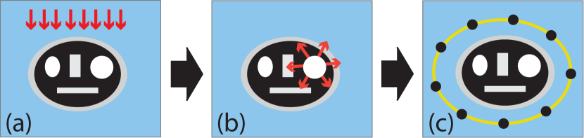
Figure 1: (a) An object is illuminated with a short optical pulse; (b) the absorbed light distribution causes an acoustic pressure; (c) the acoustic pressure is measured outside the object and used to reconstruct an image of the interior.

In this paper we consider PAT in heterogeneous acoustic media, where the acoustic pressure satisfies the wave equation

$$\frac{\partial^{2}p(\mathbf{r},t)}{\partial t^{2}}-c^{2}(\mathbf{r})\Delta_{\mathbf{r}}p(\mathbf{r},t)=\delta^{\prime}(t)\,f(\mathbf{r})\,.$$ (1)

Here $\mathbf{r}\in\mathbb{R}^{d}$ is the spatial location, $t\in\mathbb{R}$ the time variable, $\Delta_{\mathbf{r}}$ the spatial Laplacian, $c(\mathbf{r})$ the speed of sound, and $f(\mathbf{r})$ the photoacoustic (PA) source that has to be recovered. The wave equation (1) is augmented with initial condition $p(\mathbf{r},t)=0$ on $\{t<0\}$. The acoustic pressure is then uniquely defined and referred to as the causal solution of (1). Both cases $d=2,3$ for the spatial dimension are relevant in PAT: The case $d=3$ arises in PAT using classical point-wise measurements; the case $d=2$ is relevant for PAT with integrating line detectors [3, 6, 29, 28].

To recover the PA source, the pressure is measured with sensors distributed on a surface or curve outside of the sample; see Fig. 1. Using standard sensing, the spatial sampling step size limits the spatial resolution of the measured data and therefore the spatial resolution of the final reconstruction. Consequently, high spatial resolution requires a large number of detector locations. Ideally, for high frame rate, the pressure data are measured in parallel with a large array made of small detector elements. However, producing a detector array with a large number of parallel readouts is costly and technically demanding. In this work we use techniques of compressed sensing (CS) to reduce the number of required measurements and thereby accelerating PAT while keeping high spatial resolution [30, 1, 5, 20].

CS is a new sensing paradigm introduced in [8, 9, 12] that allows to capture high resolution signals using much less measurements than advised by Shannon’s sampling theory. The basic idea is to replace point samples by linear measurements, where each measurement consists of a linear combination of sensor values. It offers the ability to reduce the number of measurements while keeping high spatial resolution. One crucial ingredient enabling CS PAT is sparsity, which refers to the requirement that the unknown signal is sparse, in the sense that it has only a small number of entries that are significantly different from zero (possibly after a change of basis).

1.1 Main contributions

In this work we develop a new framework for CS PAT that allows to bring sparsity into play. Our approach is rooted in the concept of sparsifying temporal transforms developed for PAT in [30, 20] for two and three spatial dimensions. However, the approach in this present paper extends and simplifies this transform approach considerably. First, it equally applies to any detection surface and arbitrary spatial dimension. Second, the new method can even be applied to heterogenous media. In order to achieve this, we use the second time derivative applied to the pressure data as a sparsifying transform. Opposed to [30, 20], where the transform was used to sparsify the measured signals, in the present work we exploit this for obtaining sparsity in the original imaging domain.

Our new approach is based on the following. Consider the second time derivative $\partial_{t}^{2}p(\mathbf{r},t)$ of the PA pressure. We will show, that this transformed pressure again satisfies the wave equation, however with the modified PA source $c^{2}\Delta_{\mathbf{r}}f$ in place of the original PA source $f$. If the original PA source consists of smooth parts and jumps, the modified source consists of smooth parts and sparse structures; see Fig. 2 for an example. This enables the use of efficient CS reconstruction algorithms based on sparse recovery. One possible approach is based on the following two-step procedure. First, recover an approximation $h(\mathbf{r})\simeq\Delta_{\mathbf{r}}f(\mathbf{r})$ via $\ell^{1}$-minimization. In a second step, recover an approximation to $f$ by solving the Poisson equation $\Delta_{\mathbf{r}}f=h/c^{2}$.

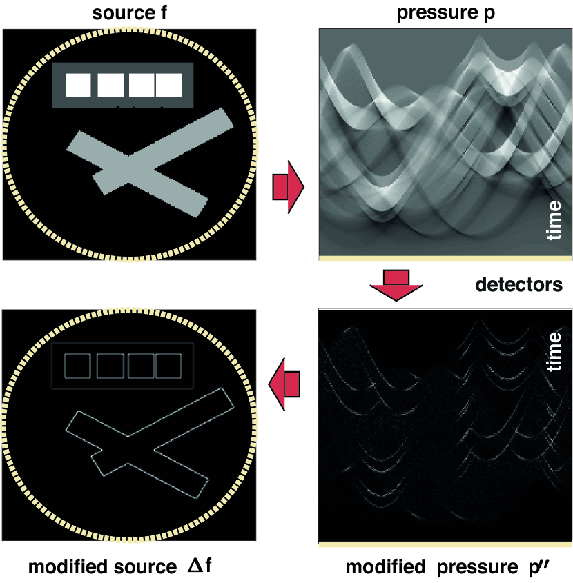
Figure 2: Top left: PA source $f$ (circle indicates the detector locations). Top right: Modified source $\Delta_{\mathbf{r}}f$. Bottom: pressure $p$ and second derivative $\partial_{t}^{2}p$ (detector locations in horizontal direction and time in vertical direction).

While the above two-stage approach turned out to very well recover the singularities of the PA source, at the same time it shows disturbing low-frequency artifacts. Therefore, in this paper we develop a completely novel strategy for jointly recovering $f$ as well as its Laplacian. It is based on solving the constrained optimization problem

$$\min_{(f,h)}\|h\|_{1}+I_{C}(f)$$

$$\text{such that }\begin{bmatrix}\mathbf{M}f,\mathbf{M}h,c^{2}\Delta_{\mathbf{r}}f-h\end{bmatrix}=\begin{bmatrix}y,y^{\prime\prime},0\end{bmatrix}\,.$$

Here $\mathbf{M}$ is the forward operator (including wave propagation and compressed measurements), $\|\cdot\|_{1}$ denotes the $\ell^{1}$-norm guaranteeing sparsity of $h$ and $I_{C}$ the indicator function of the positive cone $C\triangleq\{f\mid f(\mathbf{r})\geq 0\}$ guaranteeing non-negativity. In the case of noisy data we consider a penalized version that can be efficiently solved via various modern optimization techniques, such as forward backward splitting.

1.2 Outline

In Section 2 we describe PAT and existing CS approaches. We thereby focus on the role of sparsity in PAT. The proposed framework for CS PAT will be presented in Section 3. This includes the sparsification of the PA source and the joint reconstruction algorithm. Numerical and experimental results are presented in Section 4. The paper concludes with a summary and outlook on future research presented in Section 5.

2 Compressed photoacoustic tomography

2.1 Photoacoustic tomography

Suppose that $V\subseteq\mathbb{R}^{d}$ is a bounded region and let $\mathbf{r}_{i}$ for $i=1,\dots,n$ denote admissible detector locations distributed on the boundary $\partial V$. Then, for a given source $f$ supported inside $V$, we define

$$(\mathbf{W}f)(\mathbf{r}_{i},t)\triangleq p(\mathbf{r}_{i},t)\qquad\text{ for }i=1,\dots,n\,\text{ and }t\in[0,T]\,,$$ (2)

where $p(\mathbf{r},t)$ is the solution of (1). The inverse source problem of PAT is to recover the PA source $f$ from the $\mathbf{W}f$ in (2). The measured data $\mathbf{W}f$ is considered to be fully/completely sampled if the transducers are densely located on the whole boundary $\partial V$, such that the function $f$ can be stably reconstructed from the data. Finding necessary and sufficient sampling conditions for PAT is still on-going research [19].

Let us mention that most of the theoretical works on PAT consider the continuous setting where the transducer locations are all points of a surface or curve $\Gamma\subseteq\partial V$; see [14, 32, 24, 13, 24, 26, 17, 18, 25, 27, 21]. On the other hand, most works on discrete settings consider both discrete spatial and time variables [22, 19]. The above setting (2) has been considered in a few works [30, 20, 10]. It well reflects the high sampling rate of the time variable in many practical PAT systems.

2.2 Compressive measurements in PAT

The number $n$ of detector positions in (2) is directly related to the resolution of the final reconstruction. Namely, consider the case $V$ being the disc of radius $R$ and $f$ being essentially wavenumber limited with maximal wavenumber give by $\lambda_{0}$. Then, $N_{\varphi}\geq 2R\lambda_{0}$ equally spaced transducers are sufficient to recover $f$ with small error; see [19]. In many biomedical applications, this results in a high sampling rate. For example, the PA source may contain narrow features such as blood vessels and have sharp interfaces. This results in large wavenumbers and necessary high sampling rate. For this reason, full sampling in PAT is costly and time consuming.

To reduce the number of measurements while preserving resolution, we use CS measurements in PAT. Instead of collecting $n$ individually sampled signals as in (2), we take CS measurements

$$y(j,t)\triangleq(\mathbf{M}f)(j,t)\triangleq(\mathbf{A}\mathbf{W})(j,t)=\sum_{i=1}^{n}\mathbf{A}[j,i]p(\mathbf{r}_{i},t)\quad\text{ for }j\in\{1,\dots,m\}\,,$$ (3)

with $m\ll n$. In [7, 30] we proposed to take the measurement matrix $\mathbf{A}$ in (3) as the adjacency matrix of a lossless expander graph. Hadamard matrices have been proposed in [5, 23]. In this work, we take $\mathbf{A}$ as a random Bernoulli matrix with entries $\pm 1/\sqrt{m}$ with equal probability or a Gaussian random matrix consisting of i.i.d. $\mathcal{N}(0,{1}/{{m}})$-Gaussian random variables in each entry. These choices are validated by the fact that Gaussian and Bernoulli random matrices satisfy the restricted isometry property (RIP) with high probability (see Section 2.3 below).

2.3 The role of sparsity

A central aspect in the theory of CS is sparsity of the given data in some basis or frame [8, 12, 15]. Recall that a vector $x\in\mathbb{R}^{N}$ is called $s$-sparse if $\lvert\{i\mid x_{i}\neq 0\}\rvert\leq s$ for some number $s\ll N$, where $\lvert\,\dot{\,}\rvert$ is used to denote the number of elements of some set. If the data is known to have sparse structure, then reconstruction procedures using $\ell_{1}$-minimization or greedy-type methods can often be guaranteed to yield high quality results even if the problem is severely ill-posed [8, 16]. If we are given measurements $\mathbf{M}x=y$, where $x\in\mathbb{R}^{N}$ and $y\in\mathbb{R}^{m}$ with $m\ll N$, the success of the aforementioned reconstruction procedures can for example be guaranteed if the matrix $A$ satisfies the restricted isometry property (RIP), i.e. for all $s$-sparse vectors $z$ we have

$$(1-\delta)\|z\|^{2}\leq\|\mathbf{M}z\|^{2}\leq(1+\delta)\|z\|^{2}\,,$$ (4)

for an RIP constant $\delta<1/\sqrt{2}$; see [15]. Gaussian and Bernoulli random matrices satisfy the RIP with high probability, provided $m\geq Cs\log(\mathrm{e}n/s)$ for some reasonable constant $C$ and with $\mathrm{e}$ denoting Euler’s number [2].

In PAT, the possibility to sparsify the data has recently been examined [30, 20]. In these works it was observed that the measured pressure data could be sparsified and the sparse reconstruction methods were applied directly to the pressure data. As a second step, still a classical reconstruction via filtered backprojection had to be performed. The sparsification of the data was achieved with a transformation in the time direction of the pressure data. In two dimensions, the transform is a first order pseudo-differential operator [30], while in three dimensions the transform is of second order [20].

3 Proposed Framework

3.1 Sparsifying transform

The following theorem is the foundation of our CS approach. It shows that the required sparsity in space can be obtained by applying the second time derivative to the measured data.

Theorem 3.1.

For given source term $f\colon\mathbb{R}^{d}\to\mathbb{R}$, let $p(\mathbf{r},t)$ denote the causal solution of the wave equation (1). Then $\partial_{t}^{2}p$ is the causal solution of

$$\frac{\partial^{2}p^{\prime\prime}}{\partial t^{2}}-c^{2}(\mathbf{r})\Delta_{\mathbf{r}}p^{\prime\prime}(\mathbf{r},t)=\delta^{\prime}(t)\,c^{2}(\mathbf{r})\Delta_{\mathbf{r}}f(\mathbf{r})\,.$$ (5)

In particular, $\partial_{t}^{2}\mathbf{M}[f]=\mathbf{M}[c^{2}\Delta_{\mathbf{r}}f]$, where $\mathbf{M}$ denotes the CS PAT forward operator defined by (3).

Proof.

We first recall that the solution of (1) for $t>0$ is equivalent to the initial value problem

$$(\partial^{2}_{t}-c^{2}\Delta)p(\mathbf{r},t) =0\,,\text{ for }(\mathbf{r},t)\in\mathbb{R}^{d}\times(0,\infty)$$ (6)

$$p(\mathbf{r},0) =f(\mathbf{r})\,,\quad\text{ for }\mathbf{r}\in\mathbb{R}^{d}$$ (7)

$$\partial_{t}p(\mathbf{r},0) =0\,,\quad\text{ for }\mathbf{r}\in\mathbb{R}^{d}\,.$$ (8)

To see this equivalence note first that the solution of (6)-(8) extends to a smooth function $p\colon\mathbb{R}^{d}\times\mathbb{R}\to\mathbb{R}$ that is even in the time variable. Denoting by $\chi=\chi\{t>0\}$ the characteristic function function of $(0,\infty)$ yields $(\partial^{2}_{t}-c^{2}\Delta_{\mathbf{r}})(\chi p)=\chi(\partial^{2}_{t}-c^{2}\Delta_{\mathbf{r}})(p)+\delta^{\prime}f+2\delta(\partial_{t}p)$ Using the initial conditions (7), (8) shows that $\chi p$ (which coincides with $p$ for positive times) solves (1).

According to the above considerations, for $t>0$, the function $p$ coincides with the solution of (6)-(8). As a consequence, for $t>0$, the function $q=\partial_{t}^{2}p$ satisfies

$$(\partial^{2}_{t}-c^{2}\Delta)q(\mathbf{r},t) =0\,,\text{ for }(\mathbf{r},t)\in\mathbb{R}^{d}\times(0,\infty)$$ (9)

$$q(\mathbf{r},0) =c^{2}(\mathbf{r})\Delta_{\mathbf{r}}f(\mathbf{r})\,,\quad\text{ for }\mathbf{r}\in\mathbb{R}^{d}$$ (10)

$$\partial_{t}q(\mathbf{r},0) =0\,,\quad\text{ for }\mathbf{r}\in\mathbb{R}^{d}\,.$$ (11)

In fact, (9) results by applying the second derivative to (6) and (11) follows from the symmetry of $p$. Evaluating (6) at $t=0$ and applying the Laplacian to (7) yields initial condition (10). Finally as for the original pressure one concludes that (9)-(11) implies (5). ∎

Remark 3.1.

In order to focus on the main ideas, throughout the following we assume the spatial variable $\mathbf{r}\in\{0,\dots,N_{\mathbf{r}}\}^{d}$ to be already discretized. The discrete Laplacian $\Delta_{\mathbf{r}}$ then may be defined via symmetric finite differences; alternatively $\Delta_{\mathbf{r}}$ may be defined via the Fourier transform in the spectral domain. Theorem 3.1 and the equivalence of (1) and (6)-(8) then holds for discrete sources $f\colon\{0,\dots,N_{\mathbf{r}}\}^{d}\to\mathbb{R}$ as well.

Typical phantoms consist of smoothly varying parts and rapid changes at interfaces. For such PA sources, the modified source $c^{2}\Delta_{\mathbf{r}}f$ is sparse or at least compressible. The theory of CS therefore predicts that the modified source can be recovered by solving

$$\min_{h}\|h\|_{1}\quad\text{such that }\mathbf{M}h=\partial_{t}^{2}y\,.$$ (12)

In the case the unknown is only approximately sparse or the data are noisy, one instead minimizes the penalized functional problem $\frac{1}{2}\|\mathbf{M}h-\partial_{t}^{2}y\|_{2}^{2}+\beta\|h\|_{1}$, where $\beta>0$ is a regularization parameter which gives trade-off between the data-fitting term $\|\mathbf{M}h-\partial_{t}^{2}y\|_{2}^{2}$ and the regularization term $\|h\|_{1}$. Having obtained an approximation of $h$ by either solving (12) or the relaxed version, one can recover the original PA source $f$ by subsequently solving the Poisson equation $\Delta_{\mathbf{r}}f=h/c^{2}$ with zero boundary conditions.

While the above two-stage procedure recovers boundaries well, we observed disturbing low frequency artifacts in the reconstruction of $f$. Therefore, below we introduce a new reconstruction approach based on Theorem 3.1 that jointly recovers $f$ and $h$.

3.2 Joint reconstruction approach

As argued above, the second derivative $p^{\prime\prime}$ is well suited (via $c^{2}(\mathbf{r})\Delta_{\mathbf{r}}f$ ) to recover the singularities of $f$, but hardly contained low-frequency components of $f$. On the other hand, the low frequency information is contained in the original data, which is still available to us. Therefore we propose the following joint constrained optimization problem

$$\min_{(f,h)}\|h\|_{1}+I_{C}(f)$$ (13)

$$\text{such that }\begin{bmatrix}\mathbf{M}f,\mathbf{M}h,\Delta_{\mathbf{r}}f-h/c^{2}\end{bmatrix}=\begin{bmatrix}y,y^{\prime\prime},0\end{bmatrix}\,.$$

We habe the following result.

Theorem 3.2.

Assume that $f\colon\{0,\dots,N_{\mathbf{r}}\}^{d}\to\mathbb{R}$ is non-negative and that $\Delta_{\mathbf{r}}f$ is $s$-sparse. Moreover, suppose that the measurement matrix $\mathbf{M}$ satisfies the RIP (see (4)) and denote $y=\mathbf{M}f$. Then, the pair $[f,\Delta_{\mathbf{r}}f]$ can be recovered as the unique solution of (13).

Proof.

According to Theorem 3.1 (in a discrete form; compare Remark 3.1), $p^{\prime\prime}(\mathbf{r},t)$ is the unique causal solution of the wave equation (5) with modified source term $h=c^{2}(\mathbf{r})\Delta_{\mathbf{r}}f$. As a consequence $c^{2}(\mathbf{r})\Delta_{\mathbf{r}}h$ satisfies $\mathbf{M}h=y^{\prime\prime}$, which implies that the pair $[f,h]$ is a feasible for (13). It remains to verify that $[f,h]$ is the only solution of (13). To show this, note that for any solution $[f^{*},h^{*}]$ of (13) its second component $h^{*}$ is a solution of (12). Because $\mathbf{M}$ satisfies the $s$-RIP, and $h=c^{2}(\mathbf{r})\Delta_{\mathbf{r}}f$ is $s$-sparse, CS theory implies that (12) is uniquely solvable [8, 12, 15] and therefore $h=h^{*}$. The last constraint then implies that $f^{*}=f$. ∎

In the case the data only approximately sparse or noisy, we propose, instead of (13), to solve the $\ell^{2}$-relaxed version

$$\frac{1}{2}\|\mathbf{M}f-y\|_{2}^{2}+\frac{1}{2}\|\mathbf{M}h-y^{\prime\prime}\|_{2}^{2}+\frac{\alpha}{2}\|\Delta_{\mathbf{r}}f-h/c^{2}\|_{2}^{2}+\beta\|h\|_{1}+I_{C}(f)\to\min_{(f,h)}\,.$$ (14)

Here $\alpha>0$ is a tuning and $\beta>0$ a regularization parameter. There are several modern methods to efficiently solve (14). In this work we use the forward-backward splitting with quadratic term as smooth part used in the explicit (forward) step and $\beta\|h\|_{1}+I_{C}(f)$ as non-smooth part used for the implicit (backward) step.

3.3 Numerical minimization

We will solve (14) using a proximal gradient algorithm [11], which is an algorithm well suited for minimizing the sum of a smooth and a non-smooth but convex part. In the case of (14) we take the smooth part as

$$\Phi(f,h)\triangleq\frac{1}{2}\|\mathbf{M}f-y\|_{2}^{2}+\frac{1}{2}\|\mathbf{M}h-y^{\prime\prime}\|_{2}^{2}+\frac{\alpha}{2}\|\Delta_{\mathbf{r}}f-h/c^{2}\|_{2}^{2}$$ (15)

and the non-smooth part as $\Psi(f,h)\triangleq\beta\|h\|_{1}+I_{C}(f)$.

The proximal gradient algorithm then alternately performs an explicit gradient step for $\Phi$ and an implicit proximal step for $\Psi$. The gradient $[\nabla_{f}\Phi,\nabla_{h}\Phi]$ of the smooth part can easily be computed to be

$$\nabla_{f}\Phi(f,h) =\mathbf{M}^{*}(\mathbf{M}f-y)-\alpha\Delta_{\mathbf{r}}(\Delta_{\mathbf{r}}f-h/c^{2})$$

$$\nabla_{h}\Phi(f,h) =\mathbf{M}^{*}(\mathbf{M}h-y^{\prime\prime})-\frac{\alpha}{c^{2}}(\Delta_{\mathbf{r}}f-h/c^{2})\,.$$

The proximal map of the non-smooth part is given by

$$\mathrm{prox}(f,h) =[\mathrm{prox}_{I_{C}}(f),\mathrm{prox}_{\beta\|\cdot\|_{1}(h)}]\,,$$

$$\mathrm{prox}_{I_{C}}(f) =(\max(f_{i},0))_{i}\,,$$

$$\mathrm{prox}_{\beta\|\cdot\|_{1}}(h) =(\max(|h_{i}|-\beta,0)\,\mathrm{sign}(h_{i}))_{i}$$

With this, the proximal gradient algorithm is given by

$$f^{k+1} =\mathrm{prox}_{I_{C}}\left(f^{k}-\mu_{k}\nabla_{f}\Phi(f^{k},h^{k})\right)$$ (16)

$$h^{k+1} =\mathrm{prox}_{\beta\|\cdot\|_{1}}\left(h^{k}-\mu_{k}\nabla_{k}\Phi(f^{k},h^{k})\right),$$ (17)

where $(f^{k},h^{k})$ is the $k$-th iterate and $\mu_{k}$ the step size in the $k$-th iteration. We initialize the proximal gradient algorithm with $f^{0}=h^{0}=0$.

Remark 3.2.

Note that the optimization problem (13) is further equivalent to the analysis-$\ell_{1}$ problem

$$\min_{f}\|c\Delta_{\mathbf{r}}f\|_{1}+I_{C}(f)$$ (18)

$$\textnormal{such that }\mathbf{M}f=y\,.$$

Implementation of (18) avoids taking the second time derivative of the data $y$. Because the proximal map of $f\mapsto\|c\Delta_{\mathbf{r}}f\|_{1}$ in not available explicitly, (18) and its relaxed versions cannot be straightforwardly addressed with the proximal gradient algorithm. Therefore, in the present paper we only use the model (14) and the algorithm (16), (17) for its minimization. Different models and algorithms will be investigated in future research.

4 Experimental and numerical results

4.1 Numerical results

For the presented numerical results, the two dimensional PA source term $f\colon\{0,\dots,N_{\mathbf{r}}\}^{2}\to\mathbb{R}$ depicted in Figure 2 is used which is assumed to be supported in a disc of radius $R$. Additional results are presented using an MRI image. The synthetic data is recorded on the boundary circle of radius $R$, where the the time was discretized with $301$ equidistant sampling points in the interval $[0,2R]$. The full data was recorded at $n=200$ detector locations. The reconstruction of both phantoms via the filtered backprojection algorithm of [14] from the full measurements is shown in Figure 3.

Figure 3: Reconstructions from full data (cross phantom and MRI phantom): Reconstruction from image from 200 equispaced (fully sampled) measurements of the cross and the MRI image used in the numerical experiments.

CS measurements $\mathbf{M}f$ (see (3)) have been generated in two random ways and one deterministic way. The random matrices $\mathbf{A}$ have be taken either as random Bernoulli matrix with entries $\pm 1/{\sqrt{m}}$ with equal probability or a Gaussian random matrix consisting of i.i.d. $\mathcal{N}(0,1/{m})$-Gaussian random variables in each entry. The deterministic subsampling was performed by choosing $m$ equispaced detectors. In the joint reconstruction with (16), (17), the step-size and regularization parameters are chosen to be $\mu_{k}=0.1$, $\alpha=0.1$ and $\beta=0.005$; $5000$ iterations are performed. For the random subsampling matrices the recovery guarantees from the theory of CS can be employed, but they do not provably hold for the deterministic subsampling - although the results are equally convincing even for subsampling on the order of $10\text{\,}\mathrm{\char 37\relax}$ of the full data, cf. Figure 4. All results are compared to the standard filtered backprojection (FBP) reconstruction applied to $\mathbf{A}^{T}(\mathbf{M}f)$.

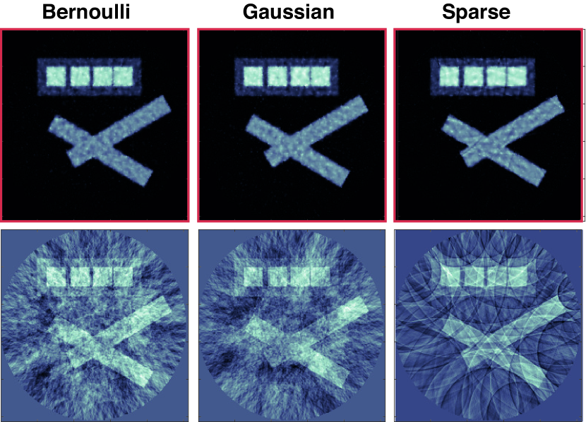
Figure 4: Reconstructions from 20 noisefree measurements (cross phantom): Reconstruction from $m=20$ noisefree CS measurements (i.e. $10\text{\,}\mathrm{\char 37\relax}$ of the fully sampled data) using the method presented in this article (top) and FBP (bottom).

If one increases the number of measurements to about $25\text{\,}\mathrm{\char 37\relax}$ of the data, the reconstruction results become almost indistinguishable from the results obtained from FBP on the full data, cf. Figure 5.

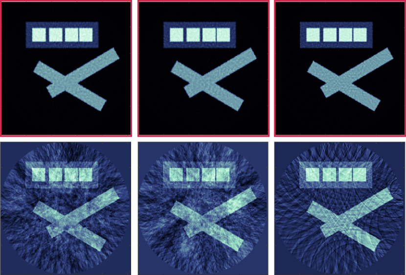
Figure 5: Reconstructions from 50 noise-free measurements (cross phantom): Reconstruction from $m=50$ (i.e. $25\text{\,}\mathrm{\char 37\relax}$ of the fully sampled data) noise-free CS measurements using the method presented in this article (top) and FBP (bottom).

In Figure 6 the application of the method developed in this article to an MRI image is presented. As the sparsity of the Laplacian is not as pronounced as in the synthetic example, the MRI image requires more measurements to achieve high qualitative outcome.

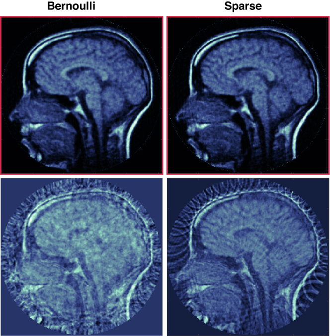
Figure 6: Reconstructions from 60 noisefree measurements (MRI phantom): Reconstruction of an MRI image from $m=60$ (i.e. $33\text{\,}\mathrm{\char 37\relax}$ of the fully sampled data) synthetically generated noisefree measurements using the method presented in this article (top) and FBP (bottom).

For noisy data, the algorithm still produces good results, although more samples need to be taken to achieve good results. For the synthetic phantom, Gaussian noise amounting to an SNR of approximately $15\text{\,}\mathrm{\char 37\relax}$ was added. The reconstruction results using $m=20$ and $m=50$ measurements are depicted in Figure 7 and Figure 8, respectively.

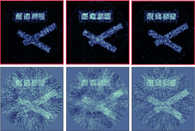
Figure 7: Reconstructions from 20 noisy measurements (cross phantom): Reconstruction from $m=20$ (i.e. $10\text{\,}\mathrm{\char 37\relax}$ of the fully sampled data) noisy measurements using the method presented in this article (top) and FBP (bottom).

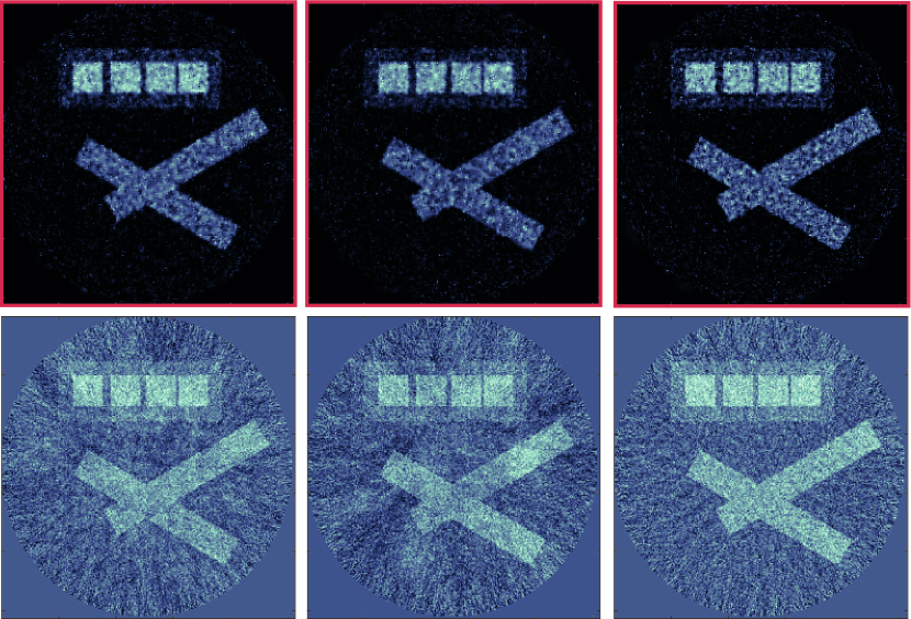
Figure 8: Reconstructions from 50 noisy measurements (cross phantom): Reconstruction from $m=50$ (i.e. $25\text{\,}\mathrm{\char 37\relax}$ of the fully sampled data) noisy measurements using the method presented in this article (top) and FBP (bottom).

4.2 Experimental results

Experimental data have been acquired by an all-optical photoacoustic projection imaging (O-PAPI) system as described in [3]. The system featured 64 integrating line detector (ILD) elements distributed along a circular arc of radius $4\text{\,}\mathrm{c}\mathrm{m}$, covering an angle of $289\text{\,}\mathrm{d}\mathrm{e}\mathrm{g}\mathrm{r}\mathrm{e}\mathrm{e}$. For an imaging depth of $20\text{\,}\mathrm{m}\mathrm{m}$, the imaging resolution of the O-PAPI system was estimated to be between $100\text{\,}\mu\mathrm{m}$ and $260\text{\,}\mu\mathrm{m}$; see [3]. PA signals were excited by illuminating the sample from two sides with pulses from a frequency-doubled Nd:YAG laser (Continuum Surelite, $20\text{\,}\mathrm{H}\mathrm{z}$ repetition rate, $6\text{\,}\mathrm{n}\mathrm{s}$ pulse duration, $532\text{\,}\mathrm{n}\mathrm{m}$ center wavelength) at a fluence of $21\text{\,}\mathrm{m}\mathrm{J}\mathrm{/}\mathrm{c}\mathrm{m}^{2}$ and recorded by the ILD elements with a sample rate of $60\text{\,}\mathrm{M}\mathrm{S}\mathrm{/}\mathrm{s}$. The sample consisted an approximately triangular shaped piece of ink-stained leaf skeleton, embedded in a cylinder consisting of agarose gel with a diameter of $36\text{\,}\mathrm{m}\mathrm{m}$ and a height of $40\text{\,}\mathrm{m}\mathrm{m}$. Intralipid was added to the agarose to increase optical scattering. The strongest branches of the leaf had diameters of approximately $160\text{\,}\mu\mathrm{m}190\text{\,}\mu\mathrm{m}$ and the smallest branches of about $50\text{\,}\mu\mathrm{m}$. Results are only for 2D (projection imaging).

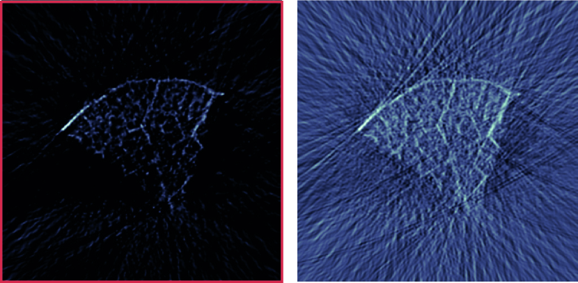
Figure 9: Reconstruction from experimental data using 60 sparse samples: Left: PAT image reconstructed with the proposed method. Right: FBP reconstruction.

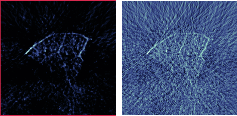
Figure 10: Reconstruction using 30 Bernoulli measurements: Left: PAT image reconstructed with the proposed method. Right: FBP reconstruction.

Reconstruction results for the leaf phantom from 60 sparsely sampled sensor locations after 500 iterations with the proposed joint minimization algorithm are shown in Figure 9. For this, the regularization and step-size parameters were chosen as in the previous section. From the experimental data we also generated $m=30$ random Bernoulli measurements. The reconstruction results using this data are shown in Figure 10. For all results, the PA source is displayed on a $1.6\text{\,}\mathrm{c}\mathrm{m}$ $\times$ $1.33\text{\,}\mathrm{c}\mathrm{m}$ rectangle with step size $26\text{\,}\mu\mathrm{m}$ inside the detection arc.

5 Conclusion

In order to achieve high spatial resolution in PAT, standard measurement and reconstruction schemes require a large number of spatial measurements with high bandwidth detectors. In order to speed up the measurement process, systems allowing a large number of parallel measurements are desirable. However such systems are technically demanding and costly to fabricate. For example, in PAT with integrating detectors, the required analog to digital converters are among the most costly building blocks. In order to increase measurement speed and to minimize system costs, CS aims to reduce the number of measurements while preserving high resolution of the reconstructed image.

One main ingredient enabling CS in PAT is sparsity of the image to be reconstructed. To bring sparsity into play, in this paper we introduced a new approach based on the commutation relation $\partial_{t}^{2}\mathbf{W}[f]=\mathbf{W}[c^{2}\Delta_{\mathbf{r}}f]$ between the PAT forward operator $\mathbf{W}$ and the the Laplacian. We developed a new reconstruction strategy for jointly reconstructing the pair $[f,\Delta_{\mathbf{r}}f]$ by minimizing (14) and thereby using sparsity of $\Delta_{\mathbf{r}}f$. The commutation relation further allows to rigorously study generalized Tikhonov regularization of the form $\frac{1}{2}\|\mathbf{M}f-y\|_{2}^{2}+\beta\|c\Delta_{\mathbf{r}}f\|_{1}+I_{C}(f)$ for CS PAT. Such an analysis as well as the development of more efficient numerical minimization schemes are subjects of further research.

References

- [1] S. Arridge, P. Beard, M. Betcke, B. Cox, N. Huynh, F. Lucka, O. Ogunlade, and E. Zhang. Accelerated high-resolution photoacoustic tomography via compressed sensing. Phys. Med. Biol., 61(24):8908, 2016.
- [2] R. Baraniuk, M. Davenport, R. DeVore, and M. Wakin. A simple proof of the restricted isometry property for random matrices. Constructive Approximation, 28(3):253–263, 2008.
- [3] J. Bauer-Marschallinger, K. Felbermayer, and T. Berer. All-optical photoacoustic projection imaging. Biomed. Opt. Express, 8(9):3938–3951, 2017.
- [4] P. Beard. Biomedical photoacoustic imaging. Interface focus, 1(4):602–631, 2011.
- [5] M. M. Betcke, B. T. Cox, N. Huynh, E. Z. Zhang, P. C. Beard, and S. R. Arridge. Acoustic wave field reconstruction from compressed measurements with application in photoacoustic tomography. IEEE Trans. Comput. Imaging, 3:710–721, 2017.
- [6] P. Burgholzer, J. Bauer-Marschallinger, H. Grün, M. Haltmeier, and G. Paltauf. Temporal back-projection algorithms for photoacoustic tomography with integrating line detectors. Inverse Probl., 23(6):S65–S80, 2007.
- [7] P. Burgholzer, M. Sandbichler, F. Krahmer, T. Berer, and M. Haltmeier. Sparsifying transformations of photoacoustic signals enabling compressed sensing algorithms. Proc. SPIE, 9708:970828–8, 2016.
- [8] E. J. Candès, J. Romberg, and T. Tao. Robust uncertainty principles: exact signal reconstruction from highly incomplete frequency information. IEEE Trans. Inf. Theory, 52(2):489–509, 2006.
- [9] E. J. Candès and T. Tao. Near-optimal signal recovery from random projections: universal encoding strategies? IEEE Trans. Inf. Theory, 52(12), 2006.
- [10] J. Chung and L. Nguyen. Motion estimation and correction in photoacoustic tomographic reconstruction. SIAM J. Imaging Sci. 10(2): 535–557, 10(1):216–242, 2017.
- [11] P. L. Combettes and J.-C. Pesquet. Proximal splitting methods in signal processing. In Fixed-point algorithms for inverse problems in science and engineering, pages 185–212. Springer, 2011.
- [12] D. L. Donoho. Compressed sensing. IEEE Trans. Inf. Theory, 52(4):1289–1306, 2006.
- [13] D. Finch, M. Haltmeier, and Rakesh. Inversion of spherical means and the wave equation in even dimensions. SIAM J. Appl. Math., 68(2):392–412, 2007.
- [14] S. K. Finch, D.and Patch and Rakesh. Determining a function from its mean values over a family of spheres. SIAM J. Math. Anal., 35(5):1213–1240 (electronic), 2004.
- [15] S. Foucart and H. Rauhut. A mathematical introduction to compressive sensing. Birkhäuser Basel, 2013.
- [16] M. Grasmair, M. Haltmeier, and O. Scherzer. Necessary and sufficient conditions for linear convergence of -regularization. Comm. Pure Appl. Math., 64(2):161–182, 2011.
- [17] M. Haltmeier. Inversion of circular means and the wave equation on convex planar domains. Computers & Mathematics with Applications. An International Journal, 65(7):1025–1036, 2013.
- [18] M. Haltmeier. Universal inversion formulas for recovering a function from spherical means. SIAM J. Math. Anal., 46(1):214–232, 2014.
- [19] M. Haltmeier. Sampling conditions for the circular radon transform. IEEE Trans. Image Process., 25(6):2910–2919, 2016.
- [20] M. Haltmeier, T. Berer, S. Moon, and P. Burgholzer. Compressed sensing and sparsity in photoacoustic tomography. J. Opt., 18(11):114004–12pp, 2016.
- [21] M. Haltmeier and L. V. Nguyen. Analysis of iterative methods in photoacoustic tomography with variable sound speed. SIAM J.Imaging Sci., 10(2):751–781, 2017.
- [22] C. Huang, K. Wang, L. Nie, and M. A. Wang, L. V.and Anastasio. Full-wave iterative image reconstruction in photoacoustic tomography with acoustically inhomogeneous media. IEEE Trans. Med. Imag., 32(6):1097–1110, 2013.
- [23] N. Huynh, E. Zhang, M. Betcke, S. Arridge, P. Beard, and B. Cox. Single-pixel optical camera for video rate ultrasonic imaging. Optica, 3(1):26–29, 2016.
- [24] L. A. Kunyansky. Explicit inversion formulae for the spherical mean Radon transform. Inverse Probl., 23(1):373–383, 2007.
- [25] F. Natterer. Photo-acoustic inversion in convex domains. Inverse Problems Imaging, 2012.
- [26] L. V. Nguyen. A family of inversion formulas in thermoacoustic tomography. Inverse Probl. Imaging, 3(4):649–675, 2009.
- [27] V. P. Palamodov. A uniform reconstruction formula in integral geometry. Inverse Probl., 28(6):065014, 2012.
- [28] G. Paltauf, P. Hartmair, G. Kovachev, and R. Nuster. Piezoelectric line detector array for photoacoustic tomography. Photoacoustics, 8:28–36, 2017.
- [29] G. Paltauf, R. Nuster, M. Haltmeier, and P. Burgholzer. Photoacoustic tomography using a Mach-Zehnder interferometer as an acoustic line detector. Appl. Opt., 46(16):3352–3358, 2007.
- [30] M. Sandbichler, F. Krahmer, T. Berer, P. Burgholzer, and M. Haltmeier. A novel compressed sensing scheme for photoacoustic tomography. SIAM J. Appl. Math., 75(6):2475–2494, 2015.
- [31] L. V. Wang. Multiscale photoacoustic microscopy and computed tomography. Nature Phot., 3(9):503–509, 2009.
- [32] M. Xu and L. V. Wang. Universal back-projection algorithm for photoacoustic computed tomography. Phys. Rev. E, 71, 2005.
- [33] M. Xu and L. V. Wang. Photoacoustic imaging in biomedicine. Rev. Sci. Instruments, 77(4):041101 (22pp), 2006.