Abstract

Learning probability distributions on the weights of neural networks (NNs) has recently proven beneficial in many applications. Bayesian methods, such as Stein variational gradient descent (SVGD), offer an elegant framework to reason about NN model uncertainty. However, by assuming independent Gaussian priors for the individual NN weights (as often applied), SVGD does not impose prior knowledge that there is often structural information (dependence) among weights. We propose efficient posterior learning of structural weight uncertainty, within an SVGD framework, by employing matrix variate Gaussian priors on NN parameters. We further investigate the learned structural uncertainty in sequential decision-making problems, including contextual bandits and reinforcement learning. Experiments on several synthetic and real datasets indicate the superiority of our model, compared with state-of-the-art methods.

1 Introduction

Deep learning has achieved state-of-the-art performance on a wide range of tasks, including image classification (Krizhevsky et al., 2012), language modeling (Sutskever et al., 2014), and game playing (Silver et al., 2016). One challenge in training deep neural networks (NNs) is that such models may overfit to the observed data, yielding over-confident decisions in learning tasks. This is partially because most NN learning only seeks a point estimate for the model parameters, failing to quantify parameter uncertainty. A natural way to ameliorate these problems is to adopt a Bayesian neural network (BNN) formulation. By imposing priors on the weights, a BNN utilizes available data to infer an approximate posterior distribution on NN parameters (MacKay, 1992). When making subsequent predictions (at test time), one performs model averaging over such learned uncertainty, effectively yielding a mixture of NN models (Gal and Ghahramani, 2016; Zhang et al., 2016; Liu and Wang, 2016; Li et al., 2016a; Chen and Zhang, 2017). BNNs have shown improved performance on modern achitectures, including convolutional and recurrent networks (Li et al., 2016b; Gan et al., 2017; Fortunato et al., 2017).

For computational convenience, traditional BNN learning typically makes two assumptions on the weight distributions: independent isotropic Gaussian distributions as priors, and fully factorized Gaussian proposals as posterior approximation when adopting variational inference (Hernández-Lobato and Adams, 2015; Blundell et al., 2015; Liu and Wang, 2016; Feng et al., 2018; Pu et al., 2017b). By examining this procedure, we note two limitations: $(\textup{\it i})$ the independent Gaussian priors can ignore the anticipated structural information between the weights, and $(\textup{\it ii})$ the factorized Gaussian posteriors can lead to unreasonable approximation errors and underestimate model uncertainty (underestimate variances).

Recent attempts have been made to overcome these two issues. For example, (Louizos and Welling, 2016; Sun et al., 2017) introduced structural priors with the matrix variate Gaussian (MVG) distribution (Gupta and Nagar, 1999) to impose dependency between weights within each layer of a BNN. Further, non-parametric variational inference methods, e.g., Stein variational gradient descent (SVGD) (Liu and Wang, 2016), iteratively transport a set of particles to approximate the target posterior distribution (without making explicit assumptions about the form of the posterior, avoiding the aforementioned factorization assumption). SVGD represents the posterior approximately in terms of a set of particles (samples), and is endowed with guarantees on the approximation accuracy when the number of particles is exactly infinity (Liu, 2017). However, since the updates within SVGD learning involve kernel computation in the parameter space of interest, the algorithm can be computationally expensive in a high-dimensional space. This becomes even worse in the case of structural priors, where a large amount of additional parameters are introduced, rendering SVGD inefficient when directly applied for posterior inference.

We propose an efficient learning scheme for accurate posterior approximation of NN weights, adopting the MVG structural prior. We provide a new perspective to unify previous structural weight uncertainty methods (Louizos and Welling, 2016; Sun et al., 2017) via the Householder flow (Tomczak and Welling, 2016). This perspective allows SVGD to approximate a target structural distribution in a lower-dimensional space, and thus is more efficient in inference. We call the proposed algorithm Structural Stein Variational Gradient Descent (S²VGD).

We investigate the use of our structural-weight-uncertainty framework for learning policies in sequential decision problems, including contextual bandits and reinforcement learning. In these models, uncertainty is particularly important because greater uncertainty on the weights typically introduces more variability into a decision made by a policy network (Kolter and Ng, 2009), naturally leading the policy to explore. As more data are observed, the uncertainty decreases, allowing the decisions made by a policy network to become more deterministic as the environment is better understood (exploitation when the policy becomes more confident). In all these models, structural weight uncertainty is inferred by our proposed S²VGD.

We conduct several experiments, first demonstrating that S²VGD yields effective performance on classic classification/regression tasks. We then focus our experiments on the motivating applications, sequential decision problems, for which accounting for NN weight uncertainty is believed to be particularly beneficial. In these applications the proposed method demonstrates particular empirical value, while also being computationally practical. The results show that structural weight uncertainty gives better expressive power to describe uncertainty driving better exploration.

2 Preliminaries

2.1 Matrix variate Gaussian distributions

The matrix variate Gaussian (MVG) distribution (Gupta and Nagar, 1999) has three parameters, describing the probability of a random matrix $\mathbf{W}\in\mathbb{R}^{\ell_{1}\times\ell_{2}}$:

$$p(\mathbf{W}) \triangleq\mathcal{MN}(\mathbf{W};\mathbf{M,U,V})$$ (1)

$$=\dfrac{\exp\left(\dfrac{1}{2}\text{tr}[\mathbf{V}^{-1}(\mathbf{W-M})^{\top}\mathbf{U^{-1}(W-M)}]\right)}{(2\pi)^{\ell_{1}\ell_{2}/2}|\mathbf{V}|^{\ell_{1}/2}|\mathbf{U}|^{\ell_{2}/2}}$$

where $\mathbf{M}\in\mathbb{R}^{\ell_{1}\times\ell_{2}}$ is the mean of the distribution. $\mathbf{U}\in\mathbb{R}^{\ell_{1}\times\ell_{1}}$ and $\mathbf{V}\in\mathbb{R}^{\ell_{2}\times\ell_{2}}$ encode covariance information for the rows and columns of $\mathbf{W}$ respectively. The MVG is closely related to the multivariate Gaussian distribution.

Lemma 1 (Golub and Van Loan (2012)).

Assume $\mathbf{W}$ follows the MVG distribution in (1), then

$$\textsf{vec}(\mathbf{W})\sim\mathcal{N}(\textsf{vec}(\mathbf{M}),\mathbf{V}\otimes\mathbf{U})$$ (2)

where vec($\mathbf{M}$) is the vectorization of $\mathbf{M}$ by stacking the columns of $\mathbf{M}$, and $\otimes$ denotes the standard Kronecker product (Golub and Van Loan, 2012).

Furthermore, a linear transformation of an MVG distribution is still an MVG distribution.

Lemma 2 (Golub and Van Loan (2012)).

Assume $\mathbf{W}$ follows the MVG distribution in (1), $\mathbf{A}\in\mathbb{R}^{\ell_{2}\times\ell_{1}},\mathbf{C}\in\mathbb{R}^{\ell_{2}\times\ell_{1}}$, then,

$$\mathbf{B} \triangleq\mathbf{AW}\sim\mathcal{MN}(\mathbf{B;AM,AUA^{\top},V})$$ (3)

$$\mathbf{B} \triangleq\mathbf{WC}\sim\mathcal{MN}(\mathbf{B;MC,U,C^{\top}VC})$$

MVG priors for BNNs

For classification and regression tasks on data $\mathcal{D}=\{{\bm{d}}_{1},\cdots,{\bm{d}}_{N}\}$, where ${\bm{d}}_{i}=\{\mathbf{x}_{i},{\bm{y}}_{i}\}$, with input $\mathbf{x}_{i}$ and output ${\bm{y}}_{i}$, an $L$-layer NN parameterizes the mapping $\{g_{\ell}\}_{\ell=1}^{L}$, defining the prediction of ${\bm{y}}_{i}$ for $\mathbf{x}_{i}$ as:

$$\hat{{\bm{y}}}_{i}=f({\bm{x}}_{i})=g_{L}\circ g_{L-1}\circ\cdots\circ g_{0}(\mathbf{x}_{i}),~{}~{}\forall i.~{}$$ (4)

where $\circ$ represents function composition, i.e., $\mathcal{A}\circ\mathcal{B}$ means $\mathcal{A}$ is evaluated on the output of $\mathcal{B}$. Each layer $g_{\ell}$ represents a nonlinear transformation. For example, with the Rectified Linear Unit (ReLU) activation function (Nair and Hinton, 2010), $g_{\ell}({\bm{x}}_{i})=\textsf{ReLU}(\mathbf{W}_{\ell}^{\top}{\bm{x}}_{i}+\mathbf{b}_{\ell})$, where $\textsf{ReLU}(x)\triangleq\max{(0,x)}$, $\mathbf{W}_{\ell}$ is the weight matrix for the $\ell$th-layer, and $\mathbf{b}_{\ell}$ the corresponding bias term.

The MVG can be adopted as a prior for the weight matrix in each layer, to impose the prior belief that there are intra-layer weight correlations,

$$~{}\mathbf{W}_{\ell}\sim\mathcal{MN}(\mathbf{W};\mathbf{0,U_{\ell},V_{\ell}}),$$ (5)

where the covariances $\mathbf{U}_{\ell},\mathbf{V}_{\ell}$ have components drawn independently from $\textsf{Inv-Gamma}(a_{0},b_{0})$. The parameters are ${\bm{\theta}}\triangleq\{\mathbf{W}_{\ell},\log\mathbf{U}_{\ell},\log\mathbf{V}_{\ell}\}$, and the above distributions represent the prior $p({\bm{\theta}})$. Our goal with BNNs is to learn layer-wise structured weight uncertainty, described by the posterior distribution $p({\bm{\theta}}|\mathcal{D})\propto p({\bm{\theta}})p(\mathcal{D}|{\bm{\theta}})$, represented below as $p$ for simplicity. When ${{\bf U}}=\sigma{\bf I}$ and ${{\bf V}}=\sigma{\bf I}$, we reduce to BNNs with independent isotropic Gaussian priors (Blundell et al., 2015).

2.2 Stein Variational Gradient Descent

SVGD considers a set of particles $\{{\bm{\theta}}_{i}\}_{i=1}^{M}$ drawn from distribution $q$, and transforms them to better match the target distribution $p$, by update:

$${\bm{\theta}}_{i} \leftarrow{\bm{\theta}}_{i}+\epsilon\phi({\bm{\theta}}_{i}),$$ (6)

$$\phi =\arg\max_{\phi\in\mathcal{F}}\left\{\dfrac{\partial}{\partial\epsilon}\textsf{KL}(q_{[\epsilon\phi]}||p)\right\},$$

where $q_{[\epsilon\phi]}$ is the updated empirical distribution, with $\epsilon$ as the step size, and $\phi$ as a function perturbation direction chosen to minimize the KL divergence between $q$ and $p$. SVGD considers $\mathcal{F}$ as the unit ball of a vector-valued reproducing kernel Hilbert space (RKHS) $\mathcal{H}$ associated with a kernel $\kappa({\bm{\theta}},{\bm{\theta}}^{\prime})$. The RBF kernel is usually used as default. It has been shown (Liu and Wang, 2016) that:

$$-\frac{\partial}{\partial\epsilon}\textsf{KL}(q_{[\epsilon\phi]}\|p)|_{\epsilon=0} =\mathbb{E}_{{\bm{\theta}}\sim q}[\Gamma_{p}\phi({\bm{\theta}})],$$ (7)

$$\text{with}~{}~{}\Gamma_{p}\phi({\bm{\theta}}) \triangleq\nabla_{{\bm{\theta}}}\log p({\bm{\theta}}|\mathcal{D})^{\top}\phi({\bm{\theta}})+\nabla_{{\bm{\theta}}}\cdot\phi({\bm{\theta}}),$$

where $\nabla_{{\bm{\theta}}}\log p({\bm{\theta}})$ denotes the derivative of the log-density of $p$; $\Gamma_{p}$ is the Stein operator. Assuming that the update function $\phi({\bm{\theta}})$ is in a RKHS with kernel $\kappa(\cdot,\cdot)$, it has been shown in (Liu and Wang, 2016) that (7) is maximized with:

$$\phi({\bm{\theta}})=\mathbb{E}_{{\bm{\theta}}\sim q}[\kappa({\bm{\theta}},{\bm{\theta}}^{\prime})\nabla_{{\bm{\theta}}}\log p({\bm{\theta}}|\mathcal{D})+\nabla_{{\bm{\theta}}}\kappa({\bm{\theta}},{\bm{\theta}}^{\prime})].$$ (8)

The expectation $\mathbb{E}_{{\bm{\theta}}\sim q}[\cdot]$ can be approximated by an empirical averaging of particles $\{{{\bm{\theta}}_{i}}\}_{i=1}^{M}$, resulting in a practical SVGD procedure as:

$$\begin{aligned} {\bm{\theta}}_{i}\leftarrow{\bm{\theta}}_{i}+\dfrac{\epsilon}{M}\sum_{j=1}^{M}\Big{[}&\kappa({\bm{\theta}}_{j},{\bm{\theta}}_{i})\nabla_{{\bm{\theta}}_{j}}\log p({\bm{\theta}}_{j}|\mathcal{D})\\ +&\nabla_{{\bm{\theta}}_{j}}\kappa({\bm{\theta}}_{j},{\bm{\theta}}_{i})\Big{]}.\end{aligned}$$ (9)

The first term to the right of the summation in (9) drives the particles ${\bm{\theta}}_{i}$ towards the high probability regions of $p$, with information sharing across similar particles. The second term repels the particles away from each other, encouraging coverage of the entire distribution. SVGD applies the updates in (9) repeatedly, and the samples move closer to the target distribution $p$ in each iteration. When using state-of-the-art stochastic gradient-based algorithms, e.g., RMSProp (Hinton et al., 2012) or Adam (Kingma and Ba, 2015), SVGD becomes a highly efficient and scalable Bayesian inference method.

Computational Issues

Applying SVGD with structured distributions for NNs has many challenges. For a weight matrix $\mathbf{W}$ of size $\ell_{1}\times\ell_{2}$, the number of parameters in ${{\bf U}}$ and ${{\bf V}}$ are $\ell_{1}^{2}$ and $\ell_{2}^{2}$, respectively. Hence, the total number of parameters ${\bm{\theta}}$ needed to describe the distribution is $\ell_{1}\ell_{2}+\ell_{1}^{2}+\ell_{2}^{2}$, compared to $\ell_{1}\ell_{2}+1$ in traditional BNNs that employ isotropic Gaussian priors and factorization.

The increase of parameter dimension by $\ell_{1}^{2}+\ell_{2}^{2}-1$ leads to significant computational overhead. The problem becomes even more severe in two aspects in calculating the kernels: $(\textup{\it i})$ The computation increases quadratically by $M(M-1)(\ell_{1}^{2}+\ell_{2}^{2}-1)/2$, $(\textup{\it ii})$ the approximation to the repelling term in (9) using limited particles can be inaccurate in high dimensions. Therefore, it is desirable to transform the MVG distribution to a lower-dimensional representation.

3 BNN & Imposition of Structure

3.1 Reparameterization of the MVG

Since the covariance matrices $\mathbf{U}$ and $\mathbf{V}$ are positive definite, we can decompose them as $\mathbf{U}=\mathbf{P}\mathbf{\Lambda}_{1}\mathbf{\Lambda}_{1}\mathbf{P}^{\top},\mathbf{V}=\mathbf{Q}\mathbf{\Lambda}_{2}\mathbf{\Lambda}_{2}\mathbf{Q}^{\top}$, where $\mathbf{P}$ and $\mathbf{Q}$ are the corresponding orthogonal matrices, $\mathbf{\Lambda}_{1}$ and $\mathbf{\Lambda}_{2}$ are diagonal matrices with positive diagonal elements. According to Lemma 2, we show the following reparameterization of MVG:

Proposition 3.

For a random matrix ${\bf C}$ following an independent Gaussian distribution:

$$\textsf{vec}{(\mathbf{C})}\sim\mathcal{N}(\cdot,~{}\mathbf{P}^{\top}{\mathbf{\Lambda}}^{-1}_{1}\mathbf{M}\mathbf{\Lambda}^{-1}_{2}\mathbf{Q},\mathbf{I}),$$ (10)

the corresponding full-covariance MVG $\mathbf{W}$ in (1) can be reparameterized as $\mathbf{W}=\mathbf{P}\mathbf{\Lambda}_{1}\mathbf{C}\mathbf{\Lambda}_{2}\mathbf{Q}^{\top}$.

The proof is in Section A of the Supplementary Material. Therefore, $\mathbf{W}$ drawn from MVG can be decomposed as the linear product of five random matrices: • ${\bf C}$ as a standard weight matrix with an independent Gaussian distribution. • $\mathbf{\Lambda}_{1}$ and $\mathbf{\Lambda}_{2}$ as the diagonal matrices, encoding the structural information within each row and column, respectively. • $\mathbf{P}$ and $\mathbf{Q}$ as orthogonal matrices, which characterize the structural information of weights between rows and columns, respectively.

3.2 MVG as Householder Flows

Based on Proposition 3, we propose a layer decomposition: the one-layer weight matrix $\mathbf{W}$ with an MVG prior can be decomposed into a linear product of five matrices, as illustrated in Figure 1(a). Our layer decomposition provides an interesting interpretation for the original MVG layer: it is equivalent to several within-layer transformations. The representations imposed in the standard weight matrix ${\bf C}$ are rotated by ${\bf P}$ and ${{\bf Q}}$, and re-weighted by ${\bf\Lambda}_{1}$ and ${\bf\Lambda}_{2}$.

(a) Layer Decomposition

(b) Householder Flow

Figure 1: Illustration of the two proposed techniques to reduce parameter size in learning the distribution of ${{\bf W}}$: (a) decomposition of ${{\bf W}}$ as a linear product of five matrices, and (b) approximation of ${\bf P}$ or ${{\bf Q}}$ as a linear product of $K$ Householder matrices. Note that each rectangle indicates a matrix, “$\times$” indicates the matrix product, and ${\bf H}$ in (b) is constructed using (12).

Note that the layer decomposition maintains similar computational complexity as the original MVG layer. To reduce the computation bottleneck in the layer decomposition, we further propose to represent ${\bf P}$ and ${{\bf Q}}$ using Householder flows (Tomczak and Welling, 2016). Formally, a Householder transformation is a linear transformation that describes a reflection about a hyperplane containing the origin. Householder flow is a series of Householder transformations.

Lemma 4 ((Sun and Bischof, 1995)).

Any orthogonal matrix ${\bf M}$ of degree K can be expressed as a Householder flow, i.e., a product of exactly $K$ nontrivial Householder matrices., i.e.,

$$\mathbf{M}={\bf H}_{K}\mathbf{H}_{K-1}\cdots{\bf H}_{1}.$$ (11)

Importantly, each Householder matrix ${\bf H}$ is constructed from a Householder vector ${\bm{v}}$ (which is orthogonal to the hyperplane):

$${\bf H}={\bf I}-2\dfrac{{\bm{v}}{\bm{v}}^{\top}}{\|{\bm{v}}\|^{2}}.$$ (12)

According to Lemma 4, ${\bf P}$ and $\mathbf{Q}$ can be represented as a product of Householder matrices $\{\mathbf{H}^{(p)}_{k}\}$ and $\{\mathbf{H}^{(q)}_{k}\}$:

$$\mathbf{P}=\mathbf{H}^{(p)}_{K}\mathbf{H}^{(p)}_{K-1}\cdots\mathbf{H}^{(p)}_{1}$$ (13)

$$\mathbf{Q}=\mathbf{H}^{(q)}_{K}\mathbf{H}^{(q)}_{K-1}\cdots\mathbf{H}^{(q)}_{1}$$

$$\mathbf{H}^{(p)}_{k}=\mathbf{I}-2{\bm{v}}^{(p)}_{k}{\bm{v}}^{(p)\top}_{k}/\left({\bm{v}}^{(p)\top}_{k}{\bm{v}}^{(p)}_{k}\right)$$

$$\mathbf{H}^{(q)}_{k}=\mathbf{I}-2{\bm{v}}^{(q)}_{k}{\bm{v}}^{(q)\top}_{k}/\left({\bm{v}}^{(q)\top}_{k}{\bm{v}}^{(q)}_{k}\right),$$

where ${\bm{v}}^{(p)}_{k}$ and ${\bm{v}}^{(q)}_{k}$ are the $k$th Householder vector for ${\bf P}$ and ${{\bf Q}}$, respectively. This is illustrated in Figure 1 (b). Note that the degree $K\leq\min\{\ell_{1},\ell_{2}\}$, with proof in Section B of Supplementary Material. In practice, $K$ is a trade-off hyperparameter, balancing the approximation accuracy and computation trade-off.

Since Householder flows allow one to represent ${\bf P}$ or ${{\bf Q}}$ as $K$ Householder vectors, the parameter sizes reduce from $\ell_{1}^{2}$ and $\ell_{2}^{2}$ to $K\ell_{1}$ and $K\ell_{2}$. Overall, we can model ${{\bf W}}$ with structured weight priors using only $(K+1)(\ell_{1}+\ell_{2})+\ell_{1}\ell_{2}$ parameters. Therefore, we can efficiently capture the structure information with only a slight increase of computational cost (i.e., $(K+1)(\ell_{1}+\ell_{2})$).

Interestingly, our method provides a unifying perspective of previous methods on learning structured weight uncertainty. In terms of prior distributions, when $K=0$ (i.e., ${\bf P}={{\bf Q}}={\bf I}$), our reparameterization reduces to (Louizos and Welling, 2016). When $K=1$, and ${\bf\Lambda}_{1}={\bf\Lambda}_{2}={\bf I}$, our reparameterization reduces to (Sun et al., 2017). In terms of posterior learning methods, when ${\bf P}={{\bf Q}}={\bf\Lambda}_{1}={\bf\Lambda}_{2}={\bf I}$ and $M>1$, S²VGD reduces to SVGD; when $M=1$, it reduces to learning an MAP solution.

3.3 Structural BNNs Revisited

We can leverage the layer decomposition and Householder flow above to construct an equivalent BNN by approximating the $\ell$th MVG layer in (5) with standard Gaussian weight matrices:

$$p(\mathbf{C}|\lambda) =\mathcal{N}\left(\mathbf{C}_{\ell};\mathbf{0},\lambda\right),$$ (14)

$$p({\bm{v}}^{(p)}_{k\ell}|\phi) =\mathcal{N}\left({\bm{v}}^{(p)}_{k\ell};\mathbf{0},\phi\mathbf{I}\right),$$

$$p({\bm{v}}^{(q)}_{k\ell}|\phi) =\mathcal{N}\left({\bm{v}}^{(q)}_{k\ell};\mathbf{0},\phi\mathbf{I}\right),$$

$$p(\mathbf{\Lambda}^{(1)}|\psi) =\mathcal{N}\left(\mathbf{\Lambda}_{\ell}^{(1)};\mathbf{0},\psi\mathbf{I}\right)$$

$$p(\mathbf{\Lambda}^{(2)}|\psi) =\mathcal{N}\left(\mathbf{\Lambda}_{\ell}^{(2)};\mathbf{0},\psi\mathbf{I}\right),$$

$$\lambda,\phi,\psi \sim\textsf{Inv-Gamma}(\cdot;a_{\ell},b_{\ell}).$$

The forms of the likelihood for the last layer are defined according to the specific applications. For regression problems on real-valued response ${\bm{y}}$:

$$\mathbf{\mathbf{y}|{\bm{x}}},{{\bf W}}_{L} \sim\mathcal{N}(\mathbf{y};f({\bm{x}},{{\bf W}}_{L}),\gamma\mathbf{I})$$ (15)

$$\gamma \sim\textsf{Inv-Gamma}(\cdot;a_{L},b_{L})~{},$$

with $f(\cdot)$ a neural network defined in (4). For classification problems on discrete labels ${\bm{y}}$:

$$\mathbf{\mathbf{y}|{\bm{x}}},{{\bf W}}_{L} \sim\textsf{Categorical}(\mathbf{y};\textsf{Softmax}(f({\bm{x}},{{\bf W}}_{L})).$$ (16)

Note that ${{\bf W}}_{L}$ can follow the same proposed techniques to reduce parameter size. Therefore, standard SVGD algorithms can be applied to sample from the posterior distribution of each model parameter. Intuitively, in SVGD the kernel function governs the interactions between particles, which employs this information to accelerate convergence and provide better performance. Similarly, the Householder flow, encoding structural information, controls the interactions between weights in each particle.

4 Sequential Decision-Making

A principal motivation for the proposed S²VGD framework is sequential decision-making, including contextual multi-arm bandits (CMABs) and Markov decision processes (MDPs). A challenge in sequential decision-making in the face of uncertainty is the exploration/exploitation trade-off: the trade-off between either taking actions that are most rewarding according to the current knowledge, or taking exploratory actions, which may be less immediately rewarding, but may lead to better-informed decisions in the future. In a Bayesian setting, the exploration/exploration trade-off is naturally addressed by imposing uncertainty into the parameters of a policy model.

4.1 CMABs and Stein Thompson Sampling

CMABs model stochastic, discrete-time and finite action-state space control problems. A CMAB is formally defined as a tuple $\mathcal{C}=\left\langle\mathcal{S},\mathcal{A},P_{s},P_{r},r\right\rangle$, where $\mathcal{S}$ is the state/context space, $\mathcal{A}$ the action/arm space, $r\in\mathbb{R}$ is the reward, $P_{s}$ and $P_{r}$ are the unknown environment distributions to draw the context and reward, respectively. At each time step $t$, the agent $(\textup{\it i})$ first observes a context ${\bm{s}}_{t}\in\mathcal{S}$, drawn i.i.d. over time from $P_{s}$; then $(\textup{\it ii})$ chooses an action at ${\bm{a}}_{t}\in\mathcal{A}$ and observes a stochastic reward $r_{t}({\bm{a}}_{t},{\bm{s}}_{t})$, which is drawn i.i.d. over time from $P_{r}(\cdot|{\bm{a}}_{t},{\bm{s}}_{t})$, conditioned on the current context and action. The agent makes decisions via a policy $\pi({\bm{a}}|{\bm{s}})$ that maps each context to a distribution over actions, yielding the probability of choosing action ${\bm{a}}$ in state ${\bm{s}}$. The goal in CMABs is to learn a policy to maximize the expected total reward in $T$ interactions: $J(\pi)=\mathbb{E}_{P_{s},\pi,P_{r}}\sum_{t=1}^{T}r_{t}$.

We represent the policy using a ${\bm{\theta}}$-parameterized neural network $\pi_{{\bm{\theta}}}({\bm{a}}|{\bm{s}})$, where MVG priors $p({\bm{\theta}})$ are employed on the weights. At each time $t$, given the past observations $\mathcal{D}_{t}\triangleq\{{\bm{d}}\}_{j=1}^{t}$, where ${\bm{d}}_{j}=({\bm{s}}_{j},{\bm{a}}_{j},r_{j})$, the posterior distribution of ${\bm{\theta}}_{t}$ is updated as $p({\bm{\theta}}_{t}|\mathcal{D}_{t})\propto\prod_{j=1}^{t}p({\bm{d}}_{j}|{\bm{\theta}})p({\bm{\theta}})$.

Thompson sampling (Thompson, 1933) is a popular method to solve CMABs (Li et al., 2011). It approximates the posterior $p({\bm{\theta}}|\mathcal{D}_{t})$ in an online manner. At each step, Thompson sampling $(\textup{\it i})$ first draws a set of parameter samples, then $(\textup{\it ii})$ picks the action by maximizing the expected reward over current step, i.e., ${\bm{a}}_{t}=\arg\max_{{\bm{a}}}\mathbb{E}_{r\sim P_{r}(\cdot|{\bm{a}},{\bm{s}}_{t};{\bm{\theta}}_{t})}r_{t}$, $(\textup{\it iii})$ collects data samples after observing the reward $r_{t}$, and $(\textup{\it iv})$ updates posterior of the policy. We apply the proposed S²VGD for the updates in the final step, and call the new procedure Stein Thompson sampling, summarized in Algorithm 1.

Note our Stein Thompson sampling is a general scheme for exploration/exploitation balance in CMABs. The techniques in (Russo et al., 2017; Kawale et al., 2015) can be adapted in this framework; we leave this for future work.

Algorithm 1 Stein Thompson Sampling

1:$\mathcal{D}=\emptyset$; initialize particles $\Theta_{0}=\{{\bm{\theta}}_{i}\}_{i=1}^{M}$;

2:for $t=0,1,2,\ldots,T$ do

3:     Receive context ${\bm{s}}_{t}\sim P_{s}$;

4:     Draw a particle $\hat{{\bm{\theta}}}^{t}$ from $\Theta_{t}$;

5:     Select ${\bm{a}}_{t}=\arg\max_{{\bm{a}}}\mathbb{E}_{r\sim P_{r}(\cdot|{\bm{a}},{\bm{s}}_{t};\hat{{\bm{\theta}}}_{t})}r_{t}$;

6:     Observe reward $r_{t}\sim P_{r}$, by performing ${\bm{a}}_{t}$;

7:     Collect observation: $\mathcal{D}_{t+1}=\mathcal{D}_{t}\cup({\bm{s}}_{t},{\bm{a}}_{t},r_{t})$;

8:     Update $\Theta_{t+1}$, according to SVGD in (9);

9:end for

4.2 MDPs and Stein Policy Gradient

An MDP is a sequential decision-making procedure in a Markovian dynamical system. It can be seen as an extension of the CMAB, by replacing the context with the notion of a system state, that may dynamically change according to the performed actions and previous state. Formally, an MDP defines a tuple $\mathcal{M}=\left\langle\mathcal{S},\mathcal{A},P_{s},P_{r},r,\gamma\right\rangle$, which is similar to a CMAB $\mathcal{C}$ except that $(\textup{\it i})$ the next state ${\bm{s}}_{t+1}$ is now conditioned on state ${\bm{s}}_{t}$ and action ${\bm{a}}_{t}$, i.e., ${\bm{s}}_{t+1}\sim P_{s}(\cdot|{\bm{s}}_{t},{\bm{a}}_{t})$; and $(\textup{\it ii})$ a discount factor $0<\gamma<1$ for the reward is considered. The goal is to find a policy $\pi({\bm{a}}|{\bm{s}})$ to maximize the discounted expected reward: $J(\pi)=\mathbb{E}_{P_{s},\pi,P_{r}}\sum_{t=1}^{T}\gamma^{t}r_{t}$.

Policy gradient (Sutton and Barto, 1998) is a family of reinforcement learning methods that solves MDPs by iteratively updating the parameters ${\bm{\theta}}$ of the policy to maximize $J({\bm{\theta}})\triangleq J(\pi_{{\bm{\theta}}}({\bm{a}}|{\bm{s}}))$. Instead of searching for a single policy parameterized by ${\bm{\theta}}$, we consider adopting an MVG prior for $p({\bm{\theta}})$, and learning its variational posterior distribution $q({\bm{\theta}})$ using S²VGD. Following (Liu et al., 2017), the objective function is modified as:

$$\max_{q}\{\mathbb{E}_{q({\bm{\theta}})}[J({\bm{\theta}})]-\alpha\textsf{KL}(q\|p)\},\vspace{-3mm}$$ (17)

where $\alpha\in[0,+\infty)$ is the temperature hyper-parameter to balance exploitation and exploration in the policy. The optimal distribution is shown to have a simple closed form (Liu et al., 2017):

$$q({\bm{\theta}})\propto\exp\left(\dfrac{1}{\alpha}J({\bm{\theta}})\right)p({\bm{\theta}}).$$ (18)

We iteratively approximate the target distribution as:

$$\triangle\mathbf{{\bm{\theta}}}_{i}=\dfrac{\epsilon}{M}\sum_{j=1}^{M}[ \nabla_{\mathbf{{\bm{\theta}}}_{j}}\left(\dfrac{1}{\alpha}J({\bm{\theta}}_{j})+\log p({\bm{\theta}}_{j})\right)\kappa({\bm{\theta}}_{i},{\bm{\theta}}_{j})$$ (19)

$$+\nabla_{\mathbf{{\bm{\theta}}}_{j}}\kappa(\mathbf{{\bm{\theta}}}_{j},\mathbf{{\bm{\theta}}}_{i})],$$

where $J({\bm{\theta}})$ can be approximated with REINFORCE (Williams, 1992) or advantage actor critic (Schulman et al., 2016).

We note two advantages of S²VGD in sequential decision-making: (i) the structural priors can characterize the flexible weight uncertainty, thus providing better exploration-exploitation when learning the policies; (ii) the efficient approximation scheme provides accurate representation of the true posterior while maintaining similar online-processing speed.

Table 1: Averaged predictions with standard deviations in terms of RMSE and log-likelihood on test sets.

5 Experiments

To demonstrate the effectiveness of our S²VGD, we first conduct experiments on the standard regression and classification tasks, with real datasets (two synthetic experiments on classification and regression are given in the Supplementary Material). The superiority of S²VGD is further demonstrated in the experiments on contextual bandits and reinforcement learning.

We compare S²VGD with related Bayesian learning algorithms, including VMG (Louizos and Welling, 2016), PBP_MV (Sun et al., 2017), and SVGD (Liu and Wang, 2016). The RMSprop optimizer is employed if there is no specific declaration. For SVGD-based methods, we use a RBF kernel $\kappa({\bm{\theta}},{\bm{\theta}}^{\prime})=\exp(-\|{\bm{\theta}}-{\bm{\theta}}^{\prime}\|_{2}^{2}/h)$, with the bandwidth set to $h=\mathtt{med}^{2}/\log M$. (Oates et al., 2016; Gorham and Mackey, 2017) Here $\mathtt{med}$ is the median of the pairwise distance between particles. The hyper-parameters $a_{\ell}=1,b_{\ell}=0.1$. The experimental codes of this paper are available at: $\mathtt{https://github.com/zhangry868/S2VGD}$.

We first study the role of hyperparameters in S²VGD: the number of Householder transformations $K$ and the number of particles $M$. This is investigated by a classification task from (Liu and Wang, 2016) on the Covertype dataset with 581,012 data points and 54 features.

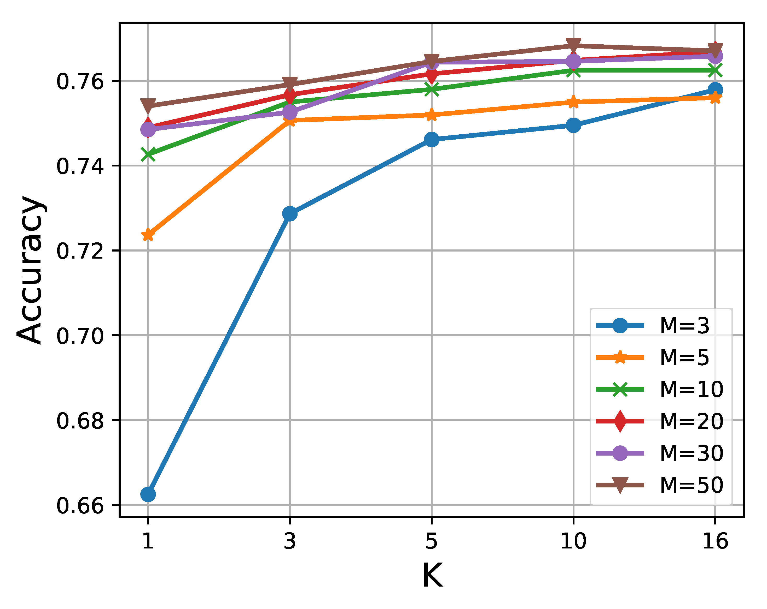
Figure 2: Impact of $K$ and $M$.

We perform 5 runs for each setting and report the mean of testing accuracy in Figure 2. As expected, increasing $M$ or $K$ improves the performance, as they lead to a more accurate approximation. Interestingly, when $M$ is small, increasing $K$ gives significant improvement. Furthermore, when $M$ is large, the change of $K$ yields similar performance. Therefore, we set $K=1$ and $M=20$ unless otherwise specified.

5.1 Regression

We use a single-layer BNN for regression tasks. Following (Li et al., 2015), 10 UCI public datasets are considered: 100 hidden units for 2 large datasets (Protein and YearPredict), and 50 hidden units for the other 8 small datasets. We repeat the experiments 20 times for all datasets except for Protein and YearPredict, which we repeat 5 times and once, respectively, for computation considerations (Sun et al., 2017). The batch size for the two large datasets is set to 1000, while it is 100 for the small datasets. The datasets are randomly split into 90% training and 10% testing. We adopt the root mean squared error (RMSE) and test log-likelihood as the evaluation criteria.

The experimental results are shown in Table LABEL:tab:reg, from which we observe that $\textup{\it i})$ weight structure information is useful (SVGD is the only method without structure, and it yields inferior performance); ii) algorithms with non-parametric assumptions, i.e., the Stein-based methods, perform better; and iii) when combined with structure information, our method achieves state-of-the-art results.

5.2 Classification

We perform the classification tasks on the standard MNIST dataset, which consists of handwritten digits of size $28\!\times\!28$, with 50,000 images for training and 10,000 for testing. A two-layer model 784-X-X-10 with ReLU activation function is used, and X is the number of hidden units for each layer. The training epoch is set to 100. The test errors for network (X-X) sizes 400-400 and 800-800 are reported in Table LABEL:tab:fnn. We observe that the Bayesian methods generally perform better than their optimization counterparts. The proposed S²VGD improves SVGD by a significant margin. Increasing $K$ also improves performance, demonstrating the advantages of incorporating structured weight uncertainty into the model. See (Li et al., 2016a; Louizos and Welling, 2016; Blundell et al., 2015) for details on the other methods with which we compare.

We wish to verify that the performance gain of S²VGD is due to the special structural design of the network architecture, rather than the increasing number of model parameters. This is demonstrated by training a NN with 415-415 hidden units using SVGD, which yields test error $1.49\%$. It has slightly more parameters than our 400-400 network trained by S²VGD (K=10), but worse performance.

Table 2: Classification error of FNN on MNIST.

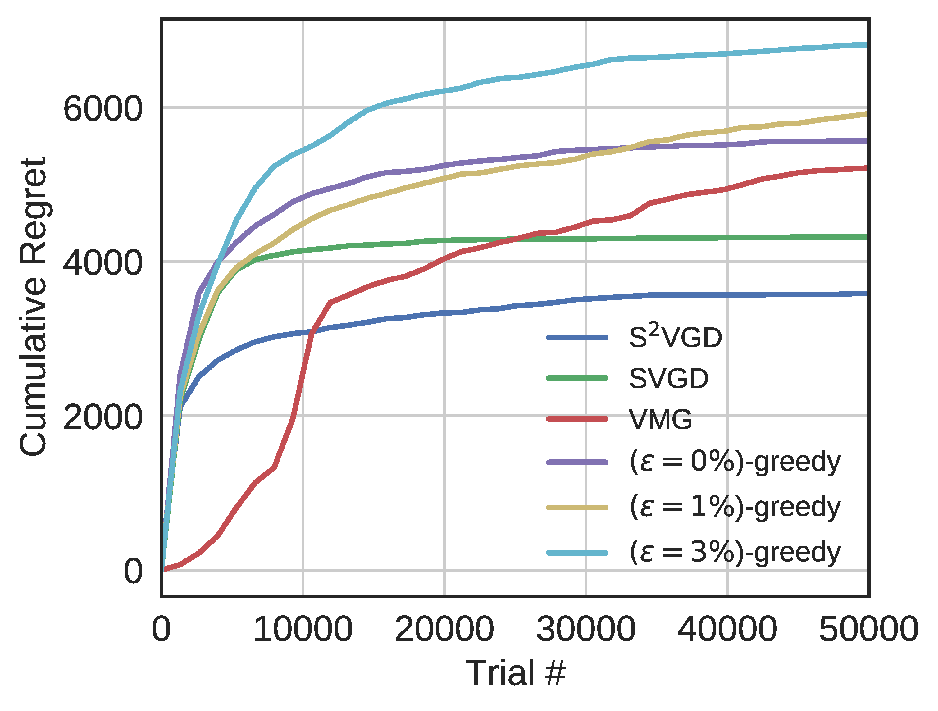
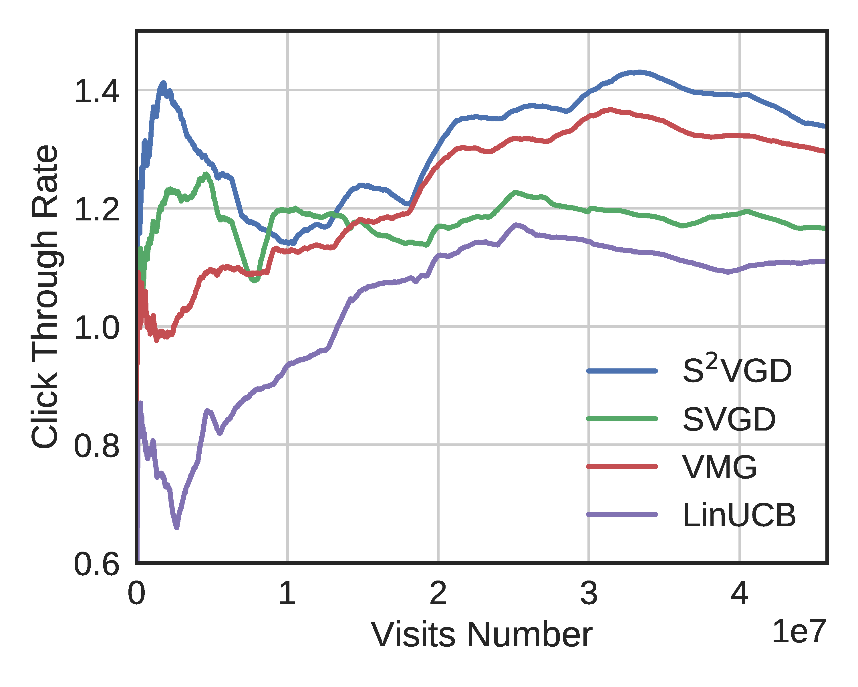
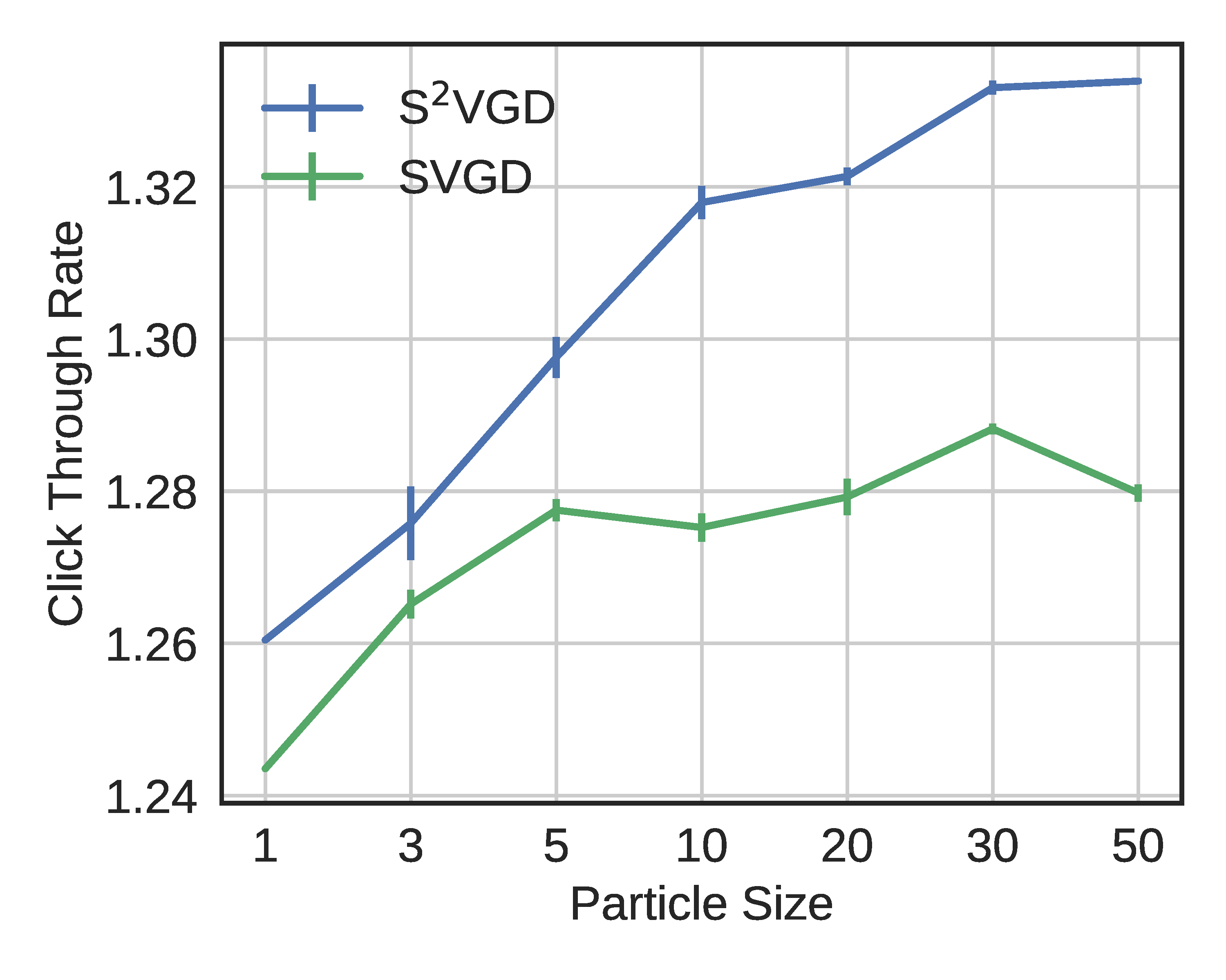
(a) Simulation results on Mushroom	(b) New Article Recommendation	(c) Particle Size on Yahoo!Today

Figure 3: Experimental results of Contextual Bandits

5.3 Contextual Bandits

Simulation

We first simulate a contextual-bandit problem with the UCI mushrooms dataset. Following (Blundell et al., 2015), the provided features of each mushroom are regarded as the context. A reward of 5 is given when an agent eats an edible mushroom. Otherwise, if a mushroom is poisonous and the agent eats it, a reward of -10 or 5 will be received, both with probability 0.5; if the agent decides not to eat the mushroom, it receives a reward of 0. We use a two-layer BNN with ReLU and 50 hidden units to represent the policy. We compared our method with a standard baseline, $\varepsilon$-greedy policy with $\varepsilon=0\%$ (pure greedy), $1\%,3\%$, respectively (Sutton and Barto, 1998).

We evaluate the performance of different algorithm by cumulative regret (Sutton and Barto, 1998), a measure of the loss caused by playing suboptimal bandit arms. The results are plotted in Figure 3(a). Thompson sampling with 3 different strategies to update policy are considered: S²VGD, SVGD and VMG. S²VGD shows lower regret at the beginning of learning than SVGD, and the lowest final cumulative regret among all methods. We hypothesize that our method captures the internal weight correlation, and the structural uncertainty can effectively help the agent learn to make less mistakes in exploration with less observations.

News Article Recommendation

We consider personalized news article recommendation on Yahoo! (Li et al., 2010), where each time a user visits the portal, a news article from a dynamic pool of candidates is recommended based on the user’s profile (context). The dataset contains 45,811,883 user visits to the Today Module in a 10-day period in May 2009. For each visit, both the user and each of the 20 candidate articles are associated with a feature vector of 6 dimensions (Li et al., 2010).

The goal is to recommend an article to a user based on its behavior, or, formally, maximize the total number of clicks on the recommended articles. The procedure is regraded as a CMAB problem, where articles are treated as arms. The reward is defined to be 1 if the article is clicked on and 0 otherwise. A one-layer NN with ReLU and 50 hidden units is used as the policy network. The classic LinUCB (Li et al., 2010) is also used as the baseline. The performance is evaluated by an unbiased offline evaluation protocol: the average normalized accumulated click-through-rate (CTR) in every 20000 observations (Li et al., 2010, 2011). The normalized CTRs are plotted in Figure 3(b). It is clear that S²VGD consistently outperforms other methods. The fact that S²VGD and VMG perform better than SVGD and the baseline LinUCB indicates that structural information helps algorithms to better balance exploration and exploitation.

To further verify the influence of the particle size $M$ on the sequential decision-making, we vary the $M$ from 1 to 50 on the-first-day data. All algorithms are repeated 10 times and their mean performances are plotted in Figure 3(c). We observe that the CTR keeps improving when $M$ becomes larger. S²VGD dominates the performance of SVGD with much higher CTRs, the gap becomes larger as $M$ increases. Since larger $M$ typically leads to more accurate posterior estimation of the policy, indicating again that the accurately learned structural uncertainty are beneficial for CMABs.

5.4 Reinforcement Learning

We apply our S²VGD to policy gradient learning. All experiments are conducted with the OpenAI $\mathtt{rllab}$ toolkit (Duan et al., 2016). Three classical continuous control tasks are considered: Cartpole Swing-Up, Double Pendulum, and Cartpole. Following the settings in (Liu et al., 2017; Houthooft et al., 2016), the policy is parameterized as a two-layer (25-10 hidden units) neural network with $\mathtt{tanh}$ as the activation function. The maximal length of horizon is set to 500. SVGD and S²VGD use a sample size of 10000 for policy gradient estimation, and $M=16$. For the easy task, Cartpole, all agents are trained for 100 episodes. For the two complex tasks, Cartpole Swing-Up and Double Pendulum, all agents are trained up to 1000 episodes. We consider two different methods to estimate the gradients: REINFORCE (Williams, 1992) and advantage actor critic (A2C) (Schulman et al., 2016)

Figure 4 plots the mean (dark curves) and standard derivation (light areas) of discounted rewards over 5 runs. In all tasks and value-estimation setups, S²VGD converges faster than SVGD and finally converges to higher average rewards. The results are even comparable to (Houthooft et al., 2016), in which a subtle reward mechanism is incorporated to encourage exploration. It demonstrates that simply adding structural information on policy networks using S²VGD improves the agent’s exploration ability. We also add a baseline method called SVGD* that applies SVGD to train a network of similar size (25-16 hidden units) with the one reparameterized by S²VGD ($K$=4). The fact that S²VGD ($K$=4) converges better than SVGD* demonstrates that our structural uncertainty is key to excellent performance.

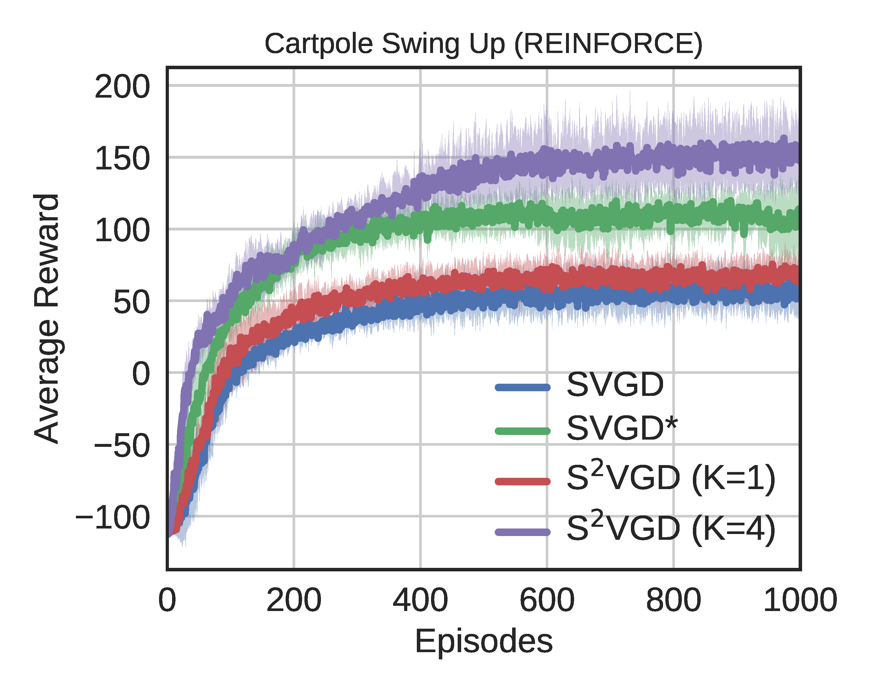
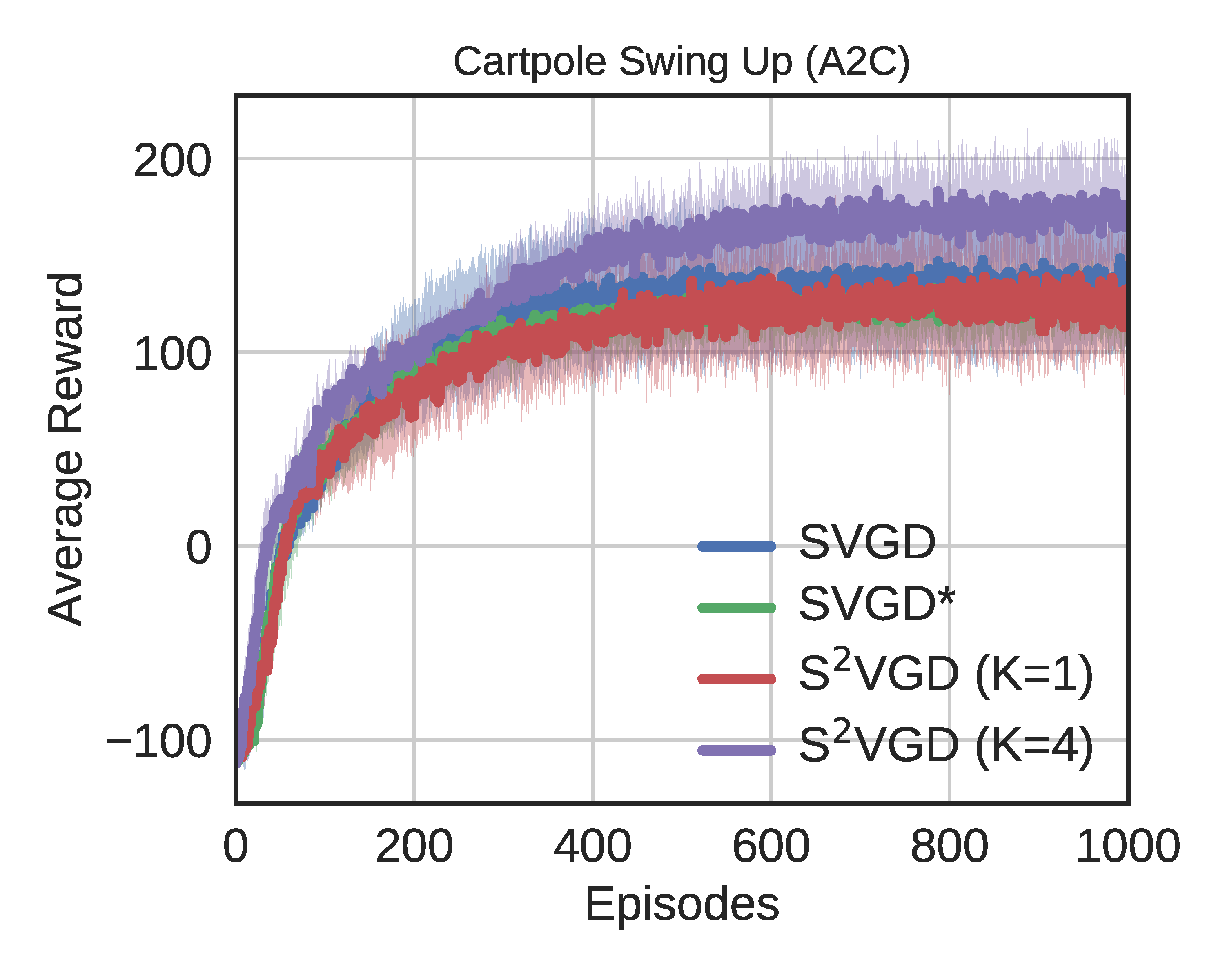
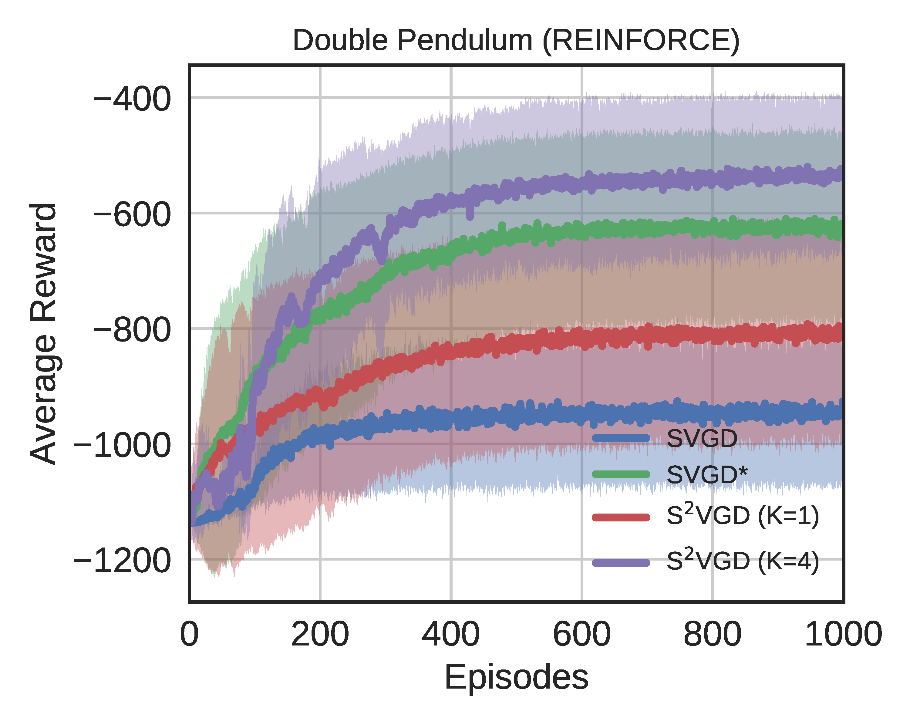
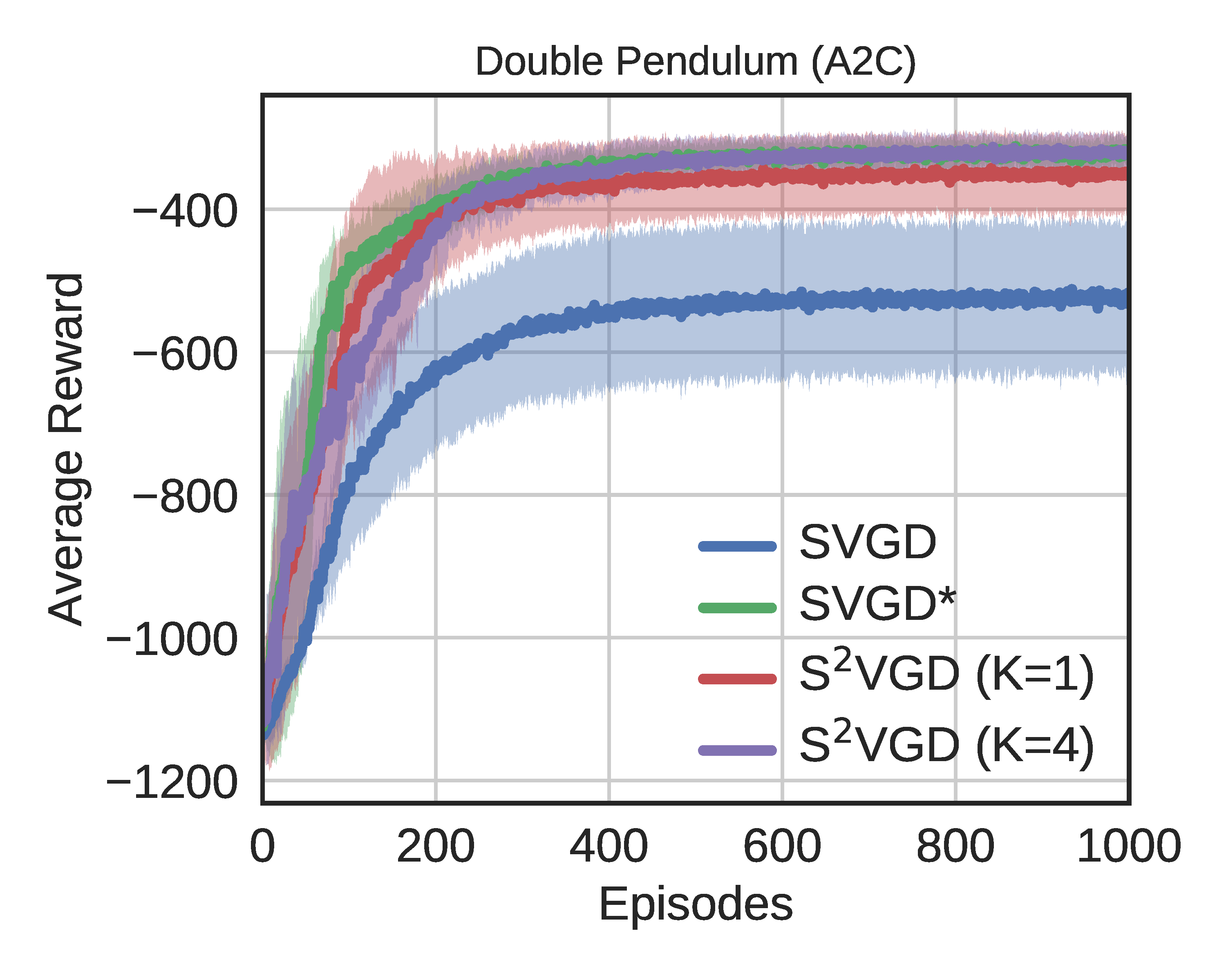
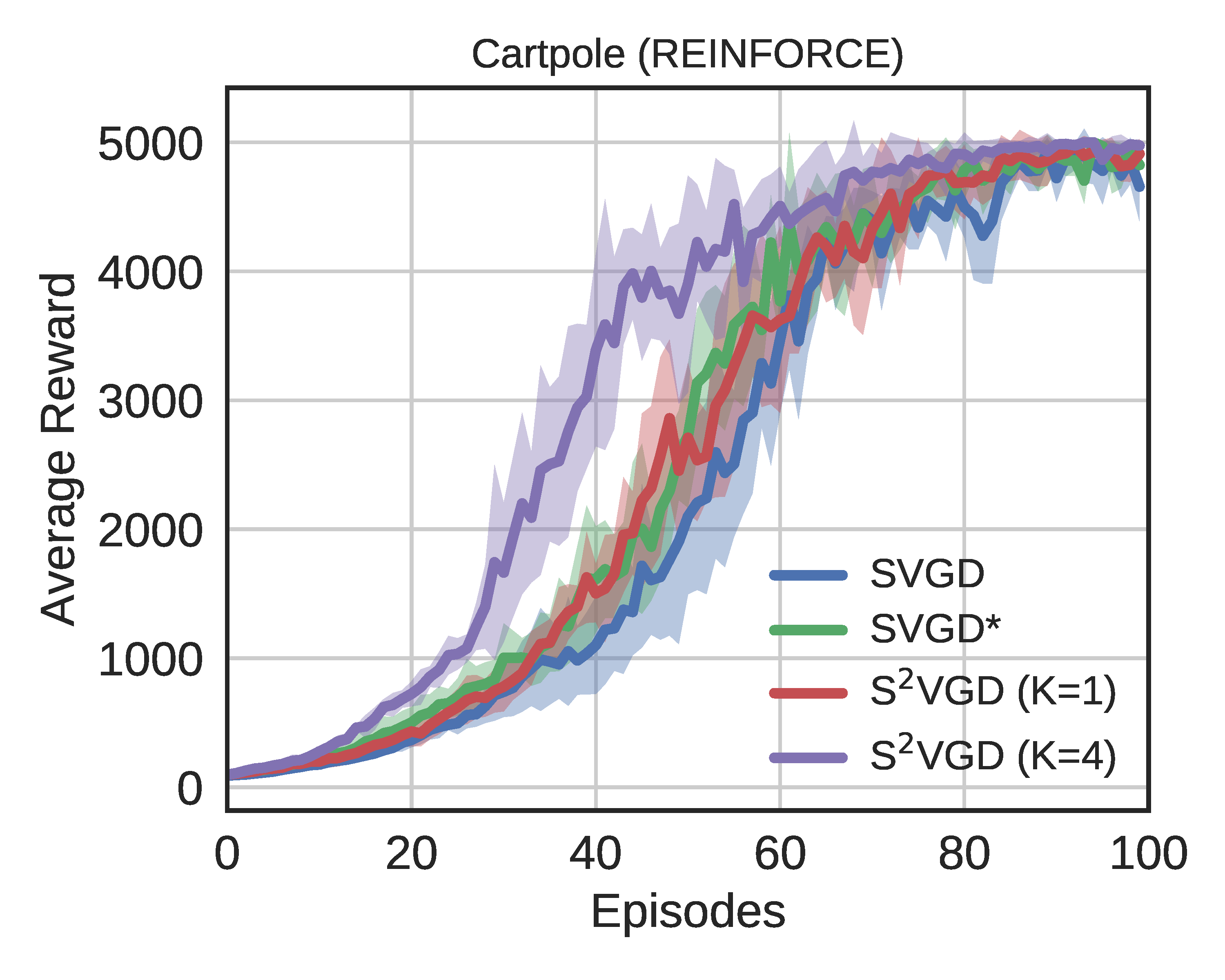
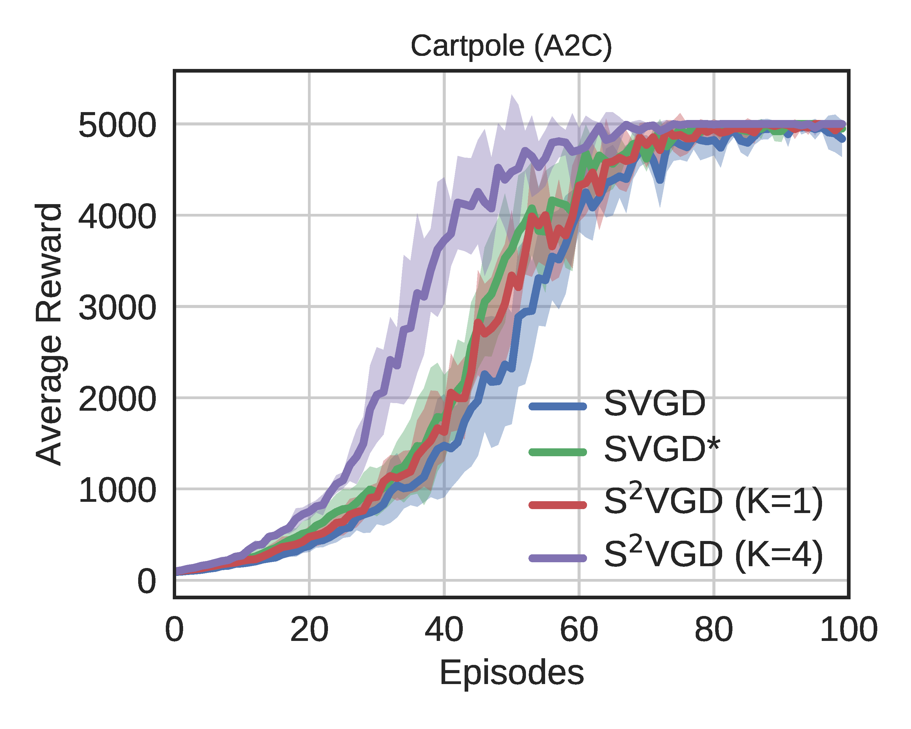
Figure 4: Learning curves by S²VGD and SVGD with REINFORCE (left) and A2C (right).

6 Conclusions

We have proposed S²VGD, an efficient Bayesian posterior learning scheme for the weights of BNNs with structural MVG priors. To achieve this, we derive a new reparametrization for the MVG to unify previous structural priors, and adopt the SVGD algorithm for accurate posterior learning. By transforming the MVG into a lower-dimensional representation, S²VGD avoids computation of related kernel matrices in high-dimensional space. The effectiveness of our framework is validated on several real-world tasks, including regression, classification, contextual bandits and reinforcement learning. Extensive experimental results demonstrate its superiority relative to related algorithms.

Our empirical results on sequential decision-making suggest the benefits of including inter-weight structure within the model, when computing policy uncertainty for online decision-making in an uncertain environments. More sophisticated methods for leveraging uncertainty for exploration/exploration balance may be a promising direction for future work. For example, explicitly encouraging exploration using learned structural uncertainty (Houthooft et al., 2016).

Acknowledgements

We acknowledge Qiang Liu and Yang Liu for making their code public. We thank Chenyang Tao for proofreading. This research was supported in part by ARO, DARPA, DOE, NGA, ONR and NSF.

 

Learning Structural Weight Uncertainty for
Sequential Decision-Making: Supplementary Material

 

Ruiyi Zhang¹   Chunyuan Li¹   Changyou Chen²   Lawrence Carin¹

¹Duke University   ²University at Buffalo ryzhang@cs.duke.edu, cl319@duke.edu, cchangyou@gmail.com, lcarin@duke.edu

Appendix A Proof of Proposition 3

Proof.

Let a MVG distributed matrix ${{\bf W}}$ be

$$~{}\mathbf{W}\sim\mathcal{MN}(\mathbf{W};\mathbf{M,U,V}),$$ (20)

Since the covariance matrices $\mathbf{U}$ and $\mathbf{V}$ are positive definite, we can decompose them as

$$\mathbf{U} =\mathbf{P}\mathbf{\Lambda}_{1}\mathbf{\Lambda}_{1}\mathbf{P}^{\top},$$ (21)

$$\mathbf{V} =\mathbf{Q}\mathbf{\Lambda}_{2}\mathbf{\Lambda}_{2}\mathbf{Q}^{\top},$$ (22)

where $\mathbf{P}$ and $\mathbf{Q}$ are the corresponding orthogonal matrices, i.e., ${\bf P}{\bf P}^{\top}={\bf I}$, ${{\bf Q}}{{\bf Q}}^{\top}={\bf I}$.

According to Lemma 2, we have,

$$~{}{\bf P}^{\top}\mathbf{W}\sim\mathcal{MN}({\bf P}^{\top}\mathbf{W};{\bf M},{\bf P}^{\top}{{\bf U}}{\bf P},{{\bf V}}),$$ (23)

Since ${{\bf U}}=\mathbf{P}\mathbf{\Lambda}_{1}\mathbf{\Lambda}_{1}\mathbf{P}^{\top}$, and we have:

$$~{}{\bf P}^{\top}\mathbf{W}\sim\mathcal{MN}({\bf P}^{\top}\mathbf{W};\mathbf{M},{\bf P}^{\top}\mathbf{P}\mathbf{\Lambda}_{1}\mathbf{\Lambda}_{1}\mathbf{P}^{\top}{\bf P},{{\bf V}}).$$ (24)

Then,

$$~{}{\bf P}^{\top}\mathbf{W}\sim\mathcal{MN}({\bf P}^{\top}\mathbf{W};\mathbf{M},\mathbf{\Lambda}_{1}\mathbf{\Lambda}_{1},{{\bf V}}),$$ (25)

Similarly, we have,

$$~{}{\bf P}^{\top}\mathbf{W}{{\bf Q}}\sim\mathcal{MN}({\bf P}^{\top}\mathbf{W}{{\bf Q}};\mathbf{M},\mathbf{\Lambda}_{1}\mathbf{\Lambda}_{1},\mathbf{\Lambda}_{2}\mathbf{\Lambda}_{2}).$$ (26)

Further,

$$~{}\mathbf{\Lambda}_{1}^{-1}{\bf P}^{\top}\mathbf{W}{{\bf Q}}\mathbf{\Lambda}_{2}^{-1}\sim\mathcal{MN}(\mathbf{\Lambda}_{1}^{-1}{\bf P}^{\top}\mathbf{W}{{\bf Q}}\mathbf{\Lambda}_{2}^{-1};\mathbf{0},{\bf I},{\bf I}),$$ (27)

Define ${\bf C}=\mathbf{\Lambda}_{1}^{-1}{\bf P}^{\top}\mathbf{W}{{\bf Q}}\mathbf{\Lambda}_{2}^{-1}$, then ${\bf C}$ follows an independent Gaussian distribution:

$${\bf C}\sim\mathcal{MN}({\bf C};\mathbf{P}^{\top}{\mathbf{\Lambda}}^{-1}_{1}\mathbf{M}\mathbf{\Lambda}^{-1}_{2}\mathbf{Q},{\bf I},{\bf I}),$$ (28)

(28) can also be expressed as:

$$\textsf{vec}{(\mathbf{C})}\sim\mathcal{N}(\textsf{vec}{(\mathbf{C})};\mathbf{P}^{\top}{\mathbf{\Lambda}}^{-1}_{1}\mathbf{M}\mathbf{\Lambda}^{-1}_{2}\mathbf{Q},\mathbf{I}),$$ (29)

showing that vectorized elements form of ${\bf C}$ follows an isotropic Gaussian distribution. Finally, since $\mathbf{\Lambda}_{1}{\bf C}\mathbf{\Lambda}_{2}$=${\bf P}^{\top}\mathbf{W}{{\bf Q}}$ , we have:

$$\mathbf{W}={\bf P}\mathbf{\Lambda}_{1}{\bf C}\mathbf{\Lambda}_{2}{{\bf Q}}^{\top}~{}.$$ (30)

∎

Appendix B Properties of Householder Flow

B.1 The Upperbound of Orthogonal Degree

Lemma 5 ([Sun and Bischof, 1995] The Basis-Kernel Representation of Orthogonal Matrices).

For any $m\times m$ orthogonal matrix ${{\bf Q}}$, there exist a full-rank $m\times k$ matrix ${\bf Y}$ and a nonsingular $k\times k$ matrix ${{\bf S}}$, $k\leq m$, such that:

$${{\bf Q}}\triangleq{{\bf Q}}({\bf Y},{{\bf S}})={\bf I}-{\bf Y}{{\bf S}}{\bf Y}^{\top}$$ (31)

Definition 6 ([Sun and Bischof, 1995] Active Subspace).

Orthogonal matrix ${{\bf Q}}$ acts on the space $\mathcal{R}({\bf Y})^{\perp}$ as the identity and changes every nonzero vector in $\mathcal{R}({\bf Y})$, and $\mathcal{R}({\bf Y})^{\perp}$ is the active space of ${{\bf Q}}$

In basis-kernel representation, ${{\bf S}}$ is the kernel, and ${\bf Y}$ is the basis. The degree of an orthogonal matrix is defined as the dimension of its active subspace. Specifically, Householder matrix is an orthogonal matrix of degree 1. With the introduced definitions and Lemma 5, the degree of an orthogonal matrix is bounded by Lemma 7.

Lemma 7 ([Sun and Bischof, 1995]).

Let $\mathbf{A}$ and $\mathbf{B}$ be two $m$-by-$k$ matrices, $k<m$. If $\mathbf{B}=\mathbf{QA}$ for some orthogonal matrix $\mathbf{Q}$, then $\mathbf{Q}$ is either of degree no greater than $k$ or can be replaced by an orthogonal factor of its own with degree no greater than $k$.

Since the degree of orthogonal matrix is bounded by size of the matrix ($k$), the number of Householder transformations needed for Householder flow is also bounded.

B.2 Intuitive Explanation

In our setting, the orthogonal matrix works as a rotation matrix. The Householder transformation reflects the weights by a hyperplane orthogonal to its corresponding Householder vector. Hence, Householder flows applies a series of reflections to the original weights. In another word, it rotates the weight matrix, equivalent to the effects of the rotation matrix.

Appendix C Computational Trick

Assume ${\bm{v}}$ is a Householder vector, and its corresponding Householder matrix ${\bf H}\triangleq{\bf I}-2\dfrac{{\bm{v}}{\bm{v}}^{\top}}{\|{\bm{v}}\|^{2}}$. For a feature vector ${\bm{x}}$, defining $\hat{{\bm{v}}}\triangleq{\bm{v}}/\|{\bm{v}}\|$, then it is easy to show:

$${\bf H}{\bm{x}} ={\bm{x}}-2\dfrac{{\bm{v}}{\bm{v}}^{\top}{\bm{x}}}{\|{\bm{v}}\|^{2}}$$ (32)

$$={\bm{x}}-2{\bm{v}}^{\top}{\bm{x}}\dfrac{{\bm{v}}}{\|{\bm{v}}\|^{2}}$$ (33)

$$={\bm{x}}-2\langle{\bm{x}},\hat{{\bm{v}}}\rangle\hat{{\bm{v}}}~{}.$$ (34)

To efficiently compute the Householder transformation, we do not need to revert the Householder matrix ${\bf H}$ and apply ${\bf H}{\bm{x}}$ to complete one Householder transformation. (32) can be used to drastically reduce the computational cost and thus make the Householder flows more efficient.

Appendix D Experimental Results

We follow the toy example in [Ghosh et al., 2016] to consider the binary classification task, in which we uniformly sample 10 data points in seperate distributions:$[-3,-1]\times[-3,-1]$ and $[1,3]\times[1,3]$. A one-layer BNNs with 30 hidden units is employed, we use at most 200 epochs for PBP_MV, SVGD and S²VGD. The posterior prediction density is plotted in Figure 5. The S²VGD performs better than other models, because it is more similar to the ground truth and has a balanced posterior density. PBP_MV employed the structure information but is a little unbalanced. The SVGD is more unbalanced compared with PBP_MV.

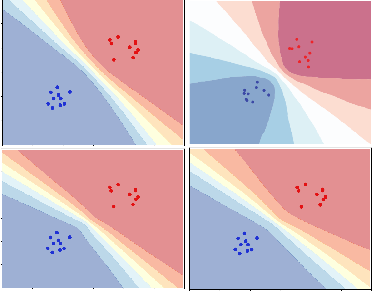
Figure 5: Binary classification on the synthetic dataset, Top left is SVGD, top right is the ground truth, bottom left is PBP_MV and bottom right is ours. The dots indicate both training and testing data points, different colors illustrates the prediction density, and the higher confidence the model has, the deeper the color will be.

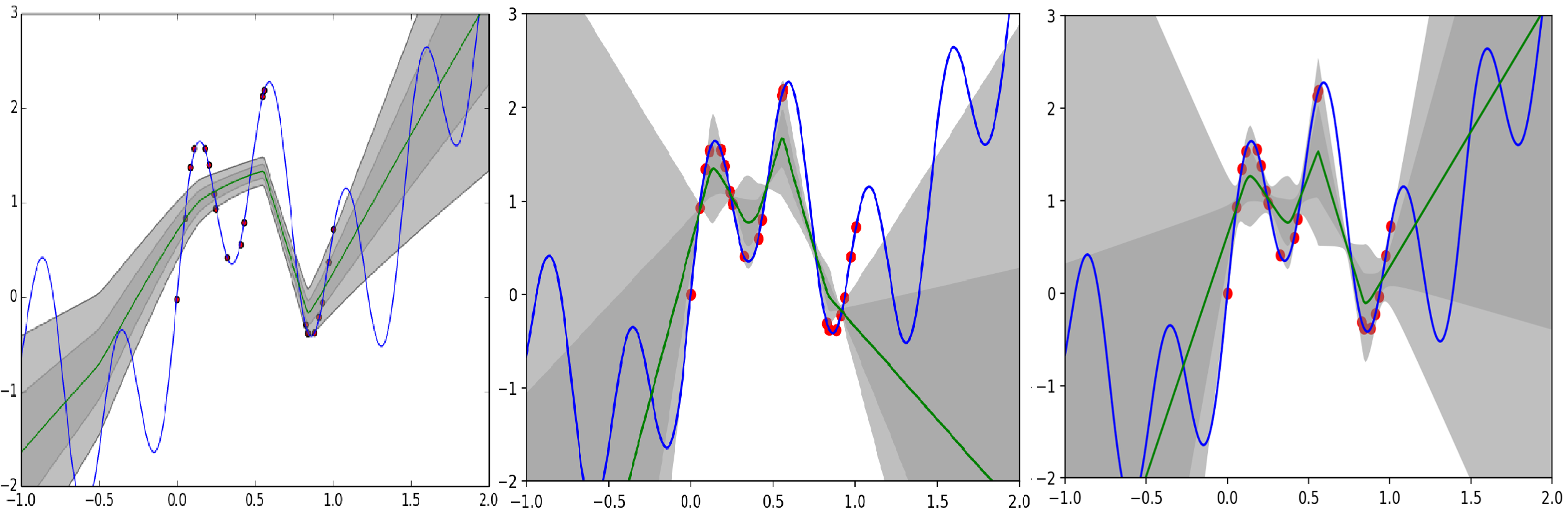
Figure 6: Regression on synthetic dataset. From the left to the right are PBP_MV, SVGD, S²VGD. The blue line is the ground truth. The light grey area shows the $\pm 3$ standard derivation confidence intervals; The green line is the mean of predictions.

For non-linear regression, we follow the experiment setup of [Louizos and Welling, 2016, Sun et al., 2017]. We randomly generated 20 points as input $x_{n}$, in which 12 points are sampled from Uniform(0,0.6), and 8 points are sampled from Uniform(0.8,1). The output $y_{n}$ is corresponding to $x_{n}$, and $y_{n}=x_{n}+\epsilon_{n}+\sin(4(x_{n}+\epsilon_{n}))+sin(13(x_{n}+\epsilon_{n}))$, where $\epsilon_{n}\sim\mathcal{N}(0,0.0009)$. We fit a one-layer ReLU neural network with 100 hidden units. We run PBP_MV, SVGD and S²VGD for at most 1500 epochs.

Compared with other methods, S²VGD captures uncertainty on two-sides using its variance, but other methods only capture part of the uncertainty.

Table 3: Hyper-parameter settings for policy gradient experiments.

Appendix E Experimental setting

We discuss the hyper-parameter settings for S²VGD, and then provide their values for our experiments. All experiments are conducted on a single TITAN X GPU.

E.1 Discussion of Hyper-parameters

Step Size

The step size $\epsilon$ for SVGD and S²VGD corresponds to the optimization counterparts. A block decay strategy is used on several datasets, it decreases by the stepsize by half every $L$ epochs.

Mini-batch Size

The gradient at step $t$ is evaluated on a batch of data $\mathcal{S}_{t}$. For small datasets, the batch size can be set to the training sample size $|\mathcal{S}_{t}|=N$, giving the true gradient for each step. For large datasets, a stochastic gradient evaluated from a mini-batch of size $|\mathcal{S}_{t}|<N$ is used to

Variance of Gaussian Prior

The prior distributions on the parameterized weights of DNNs are Gaussian, with mean 0 and variance $\sigma^{2}$. The variance of this Gaussian distribution determines the prior belief of how strongly these weights should concentrate on 0. This setting depends on user perception of the amount variability existing in the data. A larger variance in the prior leads to a wider range of weight choices, thus higher uncertainty. The weight decay value of $\ell_{2}$ regularization in stochastic optimization is related to the prior variance in SVGD and S²VGD.

Number of Particles

The number of particles $M$, is employed to approximate the posterior. SVGD and S²VGD represents the posterior approximately in terms of a set of particles (samples), and is endowed with guarantees on the approximation accuracy when the number of particles is exactly infinity [Liu, 2017]. The number of particles balanced posterior approximation accuracy and computational cost.

Number of Householder Transformations

Instead of maintaining a full orthogonal matrix, we approximate it employing householder flows containing $K$ Householder transformations. According to Lemma 4, the orthogonal matrix can be exactly represented by a series of Householder transformations, when $K$ is the degree. See details in Supplementary D. In experiments, the number of Householder transformations balanced orthogonal matrix approximation accuracy and computational cost.

E.2 Settings in Our Experiments

The hyper-parameter settings of SVGD and S²VGD on each dataset is specified in Table E.2 for MNIST, Table E.2 for contextual bandits and Table D for reinforcement learning.

Table 4: Hyper-parameter settings for contextual bandits.

Table 5: Hyper-parameter settings for MNIST.

References

- Blundell et al. (2015) Charles Blundell, Julien Cornebise, Koray Kavukcuoglu, and Daan Wierstra. Weight uncertainty in neural networks. In ICML, 2015.
- Chen and Zhang (2017) Changyou Chen and Ruiyi Zhang. Particle optimization in stochastic gradient mcmc. arXiv:1711.10927, 2017.
- Duan et al. (2016) Yan Duan, Xi Chen, Rein Houthooft, John Schulman, and Pieter Abbeel. Benchmarking deep reinforcement learning for continuous control. In ICML, 2016.
- Feng et al. (2018) Yihao Feng, Dilin Wang, and Qiang Liu. Learning to draw samples with amortized stein variational gradient descent. In UAI, 2018.
- Fortunato et al. (2017) Meire Fortunato, Charles Blundell, and Oriol Vinyals. Bayesian recurrent neural networks. arXiv:1704.02798, 2017.
- Gal and Ghahramani (2016) Yarin Gal and Zoubin Ghahramani. Dropout as a bayesian approximation: Representing model uncertainty in deep learning. In ICML, 2016.
- Gan et al. (2017) Zhe Gan, Chunyuan Li, Changyou Chen, Yunchen Pu, Qinliang Su, and Lawrence Carin. Scalable bayesian learning of recurrent neural networks for language modeling. 2017.
- Ghosh et al. (2016) Soumya Ghosh, Francesco Maria Delle Fave, and Jonathan Yedidia. Assumed density filtering methods for learning bayesian neural networks. In AAAI, 2016.
- Golub and Van Loan (2012) Gene H Golub and Charles F Van Loan. Matrix Computations. 2012.
- Gorham and Mackey (2017) Jackson Gorham and Lester Mackey. Measuring sample quality with kernels. arXiv:1703.01717, 2017.
- Gupta and Nagar (1999) Arjun K Gupta and Daya K Nagar. Matrix Variate Distributions. 1999.
- Hernández-Lobato and Adams (2015) José Miguel Hernández-Lobato and Ryan Adams. Probabilistic backpropagation for scalable learning of bayesian neural networks. In ICML, 2015.
- Hinton et al. (2012) Geoffrey E Hinton, Nitish Srivastava, and Kevin Swersky. Rmsprop: Divide the gradient by a running average of its recent magnitude. Neural Networks for Machine Learning, Coursera, 2012.
- Houthooft et al. (2016) Rein Houthooft, Xi Chen, Yan Duan, John Schulman, Filip De Turck, and Pieter Abbeel. Vime: Variational information maximizing exploration. In NIPS, 2016.
- Kawale et al. (2015) Jaya Kawale, Hung H Bui, Branislav Kveton, Long Tran-Thanh, and Sanjay Chawla. Efficient thompson sampling for online matrix-factorization recommendation. In NIPS, 2015.
- Kingma and Ba (2015) Diederik Kingma and Jimmy Ba. Adam: A method for stochastic optimization. In ICLR, 2015.
- Kolter and Ng (2009) J Zico Kolter and Andrew Y Ng. Near-bayesian exploration in polynomial time. In ICML, 2009.
- Krizhevsky et al. (2012) Alex Krizhevsky, Ilya Sutskever, and Geoffrey E Hinton. Imagenet classification with deep convolutional neural networks. In NIPS, 2012.
- Li et al. (2016a) Chunyuan Li, Changyou Chen, David E Carlson, and Lawrence Carin. Preconditioned stochastic gradient langevin dynamics for deep neural networks. In AAAI, 2016a.
- Li et al. (2016b) Chunyuan Li, Andrew Stevens, Changyou Chen, Yunchen Pu, Zhe Gan, and Lawrence Carin. Learning weight uncertainty with stochastic gradient mcmc for shape classification. In CVPR, 2016b.
- Li et al. (2010) Lihong Li, Wei Chu, John Langford, and Robert E Schapire. A contextual-bandit approach to personalized news article recommendation. In WWW, 2010.
- Li et al. (2011) Lihong Li, Wei Chu, John Langford, and Xuanhui Wang. Unbiased offline evaluation of contextual-bandit-based news article recommendation algorithms. In WSDM, 2011.
- Li et al. (2015) Yingzhen Li, José Miguel Hernández-Lobato, and Richard E Turner. Stochastic expectation propagation. In NIPS, 2015.
- Liu (2017) Qiang Liu. Stein variational gradient descent as gradient flow. In NIPS, 2017.
- Liu and Wang (2016) Qiang Liu and Dilin Wang. Stein variational gradient descent: A general purpose bayesian inference algorithm. In NIPS, 2016.
- Liu et al. (2017) Yang Liu, Prajit Ramachandran, Qiang Liu, and Jian Peng. Stein variational policy gradient. In UAI, 2017.
- Louizos and Welling (2016) Christos Louizos and Max Welling. Structured and efficient variational deep learning with matrix gaussian posteriors. In NIPS, 2016.
- MacKay (1992) David JC MacKay. A practical bayesian framework for backpropagation networks. Neural Computation, 1992.
- Nair and Hinton (2010) Vinod Nair and Geoffrey E Hinton. Rectified linear units improve restricted boltzmann machines. In ICML, 2010.
- Oates et al. (2016) Chris J Oates, Jon Cockayne, François-Xavier Briol, and Mark Girolami. Convergence rates for a class of estimators based on stein’s identity. arXiv:1603.03220, 2016.
- Pu et al. (2017a) Yunchen Pu, Liqun Chen, Shuyang Dai, Weiyao Wang, Chunyuan Li, and Lawrence Carin. Symmetric variational autoencoder and connections to adversarial learning. 2017a.
- Pu et al. (2017b) Yunchen Pu, Zhe Gan, Ricardo Henao, Chunyuan Li, Shaobo Han, and Lawrence Carin. Stein variational autoencoder. In NIPS, 2017b.
- Russo et al. (2017) Daniel Russo, David Tse, and Benjamin Van Roy. Time-sensitive bandit learning and satisficing thompson sampling. arXiv:1704.09028, 2017.
- Schulman et al. (2016) John Schulman, Philipp Moritz, Sergey Levine, Michael Jordan, and Pieter Abbeel. High-dimensional continuous control using generalized advantage estimation. In ICLR, 2016.
- Silver et al. (2016) David Silver, Aja Huang, et al. Mastering the game of go with deep neural networks and tree search. Nature, 2016.
- Sun et al. (2017) Shengyang Sun, Changyou Chen, and Lawrence Carin. Learning structured weight uncertainty in bayesian neural networks. In AISTATS, 2017.
- Sun and Bischof (1995) Xiaobai Sun and Christian Bischof. A basis-kernel representation of orthogonal matrices. SIAM Journal on Matrix Analysis and Applications, 1995.
- Sutskever et al. (2014) Ilya Sutskever, Oriol Vinyals, and Quoc V Le. Sequence to sequence learning with neural networks. In NIPS, 2014.
- Sutton and Barto (1998) Richard S Sutton and Andrew G Barto. Reinforcement learning: An introduction. 1998.
- Thompson (1933) William R Thompson. On the likelihood that one unknown probability exceeds another in view of the evidence of two samples. Biometrika, 1933.
- Tomczak and Welling (2016) Jakub M Tomczak and Max Welling. Improving variational auto-encoders using householder flow. arXiv:1611.09630, 2016.
- Williams (1992) Ronald J Williams. Simple statistical gradient-following algorithms for connectionist reinforcement learning. Machine Learning, 1992.
- Zhang et al. (2016) Yizhe Zhang, Xiangyu Wang, Changyou Chen, Ricardo Henao, Kai Fan, and Lawrence Carin. Towards unifying hamiltonian monte carlo and slice sampling. In NIPS, 2016.
- Zhang et al. (2017) Yizhe Zhang, Changyou Chen, Zhe Gan, Ricardo Henao, and Lawrence Carin. Stochastic gradient monomial gamma sampler. In ICML, 2017.