galaxies: evolution — galaxies: formation — galaxies: high-redshift — intergalactic medium — dark ages, reionization, first stars
SILVERRUSH. VI. A simulation of Ly emitters in the reionization epoch and a comparison with Subaru Hyper Suprime-Cam survey early data
Abstract
The survey of Lyman emitters (LAEs) with Subaru Hyper Suprime-Cam, called SILVERRUSH (Ouchi et al.), is producing massive data of LAEs at . Here we present LAE simulations to compare the SILVERRUSH data. In 1623 comoving Mpc3 boxes, where numerical radiative transfer calculations of reionization were performed, LAEs have been modeled with physically motivated analytic recipes as a function of halo mass. We have examined models depending on the presence or absence of dispersion of halo Ly emissivity, dispersion of the halo Ly optical depth, , and halo mass dependence of . The unique free parameter in our model, a pivot value of , is calibrated so as to reproduce the Ly luminosity function (LF) of SILVERRUSH. We compare our model predictions with Ly LFs at and , LAE angular auto-correlation functions (ACFs) at and , and LAE fractions in Lyman break galaxies at . The Ly LFs and ACFs are reproduced by multiple models, but the LAE fraction turns out to be the most critical test. The dispersion of and the halo mass dependence of are essential to explain all observations reasonably. Therefore, a simple model of one-to-one correspondence between halo mass and Ly luminosity with a constant Ly escape fraction has been ruled out. Based on our best model, we present a formula to estimate the intergalactic neutral hydrogen fraction, , from the observed Ly luminosity density at . We finally obtain as a volume-average at .
1 Introduction
Cosmic reionization is one of the central issues in modern astronomy. Understanding this major phase transition in the early Universe is closely related to the formation of the first generation of galaxies. There are three key questions to understand reionization: the history, sources and topology. The epoch of reionization is constrained to the redshift range of by the Gunn-Peterson trough found in distant QSO spectra (e.g., [Fan et al. (2006)]) and the Thomson scattering optical depth measured from polarization in the Cosmic Microwave Background (CMB) (e.g., [Planck Collaboration (2014)]). However, constraints on the evolution of the hydrogen neutral fraction, , in the intergalactic medium (IGM) during the epoch are still weak (Greig & Mesinger, 2017). Leading candidates of reionization sources are star-forming galaxies if they inject of the produced Lyman continuum into the IGM (e.g., Inoue et al. (2006)). However, this escape fraction, , of the Lyman continuum is uncertain, while efforts to measure or constrain directly (e.g., Micheva et al. (2017)) and indirectly (e.g., Khaire et al. (2016)) are on-going. There are two major types of the reionization topology: inside-out (Iliev et al., 2006) and outside-in (Miralda-Escudé et al., 2000). The topology may depend on the types of the dominant ionizing sources, i.e. galaxies or AGNs, owing to the difference of the mean-free-path (or mean energy) of ionizing photons. In theoretical models, it also depends on the treatment of recombination (Choudhury et al., 2009). Currently, it is unknown yet which topology was realized in the real Universe.
Lyman emitters (LAEs) are considered to be a useful probe of reionization because Ly is the resonant line of neutral hydrogen and sensitive to (e.g., Dijkstra (2014)). A decrease in Ly luminosity functions (LFs) at following the no evolution at (Ouchi et al., 2008) is interpreted as an increase in at due to reionization (Kashikawa et al., 2006, 2011; Ouchi et al., 2010; Ota et al., 2010; Shibuya et al., 2012; Konno et al., 2014). A decrease of the LAE number fraction in Lyman break galaxies (LBGs) at is also interpreted as a reionization signature (Stark et al., 2010, 2011; Ono et al., 2012; Schenker et al., 2013; Furusawa et al., 2016). In the inside-out reionization scenario, the clustering of LAEs is expected to be enhanced as increases (McQuinn et al., 2007). Ouchi et al. (2010) compared the observed LAE angular correlation functions (ACFs) with the model prediction by McQuinn et al. (2007) and put a constraint on the neutral hydrogen fraction of the IGM as at .
There is further progress in LAE surveys at . Ota et al. (2017) has performed the deepest survey of LAEs at with Subaru/Suprime-Cam and confirmed a decrease of the Ly LF at compared to those at and . On the other hand, Zheng et al. (2017) has reported no difference in the bright-end of the Ly LF () between and based on the widest survey of LAEs at so far with DECam on the NOAO/CTIO 4 m Blanco Telescope. Clearly, wider and deeper LAE surveys are required to settle the issue. Hyper Suprime-Cam (HSC; Miyazaki et al. (2012, 2018); Komiyama et al. (2018); Kawanomoto et al. (2017); Furusawa et al. (2018)) mounted on the 8.2 m Subaru Telescope is the most ideal instrument for such surveys. Indeed, we are conducting surveys of LAEs at , and , called Systematic Identification of LAEs for Visible Exploration and Reionization Research Using Subaru HSC (SILVERRUSH; Ouchi et al. (2018)), under the Subaru Strategic Program with HSC (Aihara et al., 2018). Early data results are already available in a series of papers (Ouchi et al., 2018; Shibuya et al., 2018a, b; Konno et al., 2018; Harikane et al., 2018b; Higuchi et al., 2018). We are also conducting additional HSC narrowband observations including an LAE survey at (Itoh et al., 2018), called CHORUS (Cosmic HydrOgen Reionization Unveiled with Subaru; Inoue et al. in prep.).
To interpret SILVERRUSH and CHORUS data and deduce the information of reionization, we need to make use of a model of LAEs in that epoch. In literature, there are many such models adopting a range of simplification (e.g., McQuinn et al. (2007); Iliev et al. (2008); Kobayashi et al. (2010); Zheng et al. (2010); Dayal et al. (2011); Jensen et al. (2013); Kakiichi et al. (2016)). For example, works with a large-scale ( comoving Mpc) and full numerical radiative transfer simulation of reionization tend to adopt a simplified LAE model assuming one-to-one correspondence between halo mass and Ly luminosity with a constant Ly escape fraction (e.g., McQuinn et al. (2007); Iliev et al. (2008); Jensen et al. (2013); Kakiichi et al. (2016)). On the other hand, works with a detailed modeling of LAEs tend to adopt a simplified or no radiative transfer simulation of reionization (e.g., Kobayashi et al. (2010); Dayal et al. (2011)). Zheng et al. (2010) simulated Ly photon transfer in galaxy halos and the circum-galactic medium (CGM) in a large-scale reionization simulation although the Ly transfer in the interstellar medium (ISM) of galaxies was not resolved. This is still difficult even today.
This work presents a new LAE simulation adopting a more physically realistic LAE model in a large-scale full numerical radiative transfer simulation of reionization to be compared with SILVERRUSH data. Such a model is essential when using LAEs as a probe of reionization but overlooked so far. We will examine validity of the assumption of one-to-one correspondence between halo mass and Ly luminosity often adopted in literature and rule out it after comparisons with early data of SILVERRUSH.
The structure of this paper is as follows; In §2, we describe the reionization simulations consisting of radiation hydrodynamics simulations to produce models of halos’ emissivity and the IGM clumping factor, N-body simulations to produce the density structure in the IGM as well as the halo distribution, and radiative transfer simulations to compute the neutral hydrogen distribution in the IGM. In §3, we make LAE models depending on the presence or absence of fluctuation in the Ly production, fluctuation in the ISM/CGM opacity for Ly, and halo mass dependence of the opacity. In §4, we show the comparisons of the simulations with early data of SILVERRUSH and identify the best model among the models. In §5, we discuss the nature of LAEs in the reionization era expected from the best model and how to constrain the reionization history with LAEs. The last section is devoted to our conclusions.
2 Reionization simulation
To model LAEs, we need to know the neutral hydrogen (H i) distribution in the IGM which affects the observability of LAEs. In this paper, we adopt a large-scale reionization simulation by Hasegawa et al. (in prep.) for the H i distribution. Since the star formation rates and ionizing photon escape fractions of galaxies are regulated by radiative feedback (Umemura et al., 2012; Hasegawa & Semelin, 2013), high resolution radiation hydrodynamics (RHD) simulations are desirable for simulating reionization. However, the volume of a cosmological RHD simulation is generally limited due to expensive numerical costs. Therefore, Hasegawa et al. adopted a two-step approach. First, they performed a cosmological RHD simulation in a computationally feasible box size to model galaxies and the IGM clumping factor under the influence of the radiative feedback (Hasegawa et al., 2016). Using the RHD models of galaxies/IGM, then, they solved radiative transfer of ionizing photons in a large-scale -body simulation box to obtain the cosmological distribution of . In the following, we briefly describe the simulations, while a full description is presented in Hasegawa et al. (in prep.). Some information can be also found in Hasegawa et al. (2016), Kubota et al. (2017) and Yoshiura et al. (2018).
2.1 Radiative hydrodynamics simulations for making recipes
The RHD simulation was performed with particles in a 20 comoving Mpc3 box. The implemented physical processes in the RHD simulation are similar to those in Hasegawa & Semelin (2013), except for the following two points: (i) stellar age dependent spectra of PÉGASE2 (Fioc & Rocca-Volmerange, 1997) 111http://www2.iap.fr/users/fioc/PEGASE.html and (ii) attenuation by dust grains (Draine & Lee, 1984) 222https://www.astro.princeton.edu/ draine/dust/dust.html.
The halo ionizing emissivity recipe is described as a look-up table of average escaping Lyman continuum spectra () as a function of halo mass and its local ionization degree obtained from the RHD simulation. The look-up table spectra already includes the escape fraction depending on the wavelength. It is worth mentioning that the contribution from massive galaxies is less dominant compared to previous reionization simulations (e.g., Iliev et al. (2006)), because the RHD simulation shows that the escape fraction decreases with increasing halo mass (Hasegawa & Semelin, 2013; Hasegawa et al., 2016; Xu et al., 2016): 10%, 2% and 0.2% at , and M⊙, respectively. The values are very consistent with those in a higher resolution RHD simulation by Xu et al. (2016) for halos less than M⊙ which they examined.
The clumping factor, defined as with being the volume average, is an important parameter regulating the recombination time-scale in reionization simulations. Previous studies on the clumping factor have shown that it becomes on average by photo-heating during reionization (Pawlik & Schaye, 2009; Finlator et al., 2012). Hasegawa et al. (2016) revisited the influence of the radiative feedback on the clumping factor and found that it depends on the density and ionization degree locally. Therefore, a spatially constant clumping factor is not correct. Hence, based on the RHD simulation, Hasegawa et al. (in prep.) made a look-up table for the local clumping factor as a function of the local density and the local ionization degree within comoving Mpc scale, corresponding to the grid size of the post-processing radiative transfer described later in §2.2.2. The clumping factor is larger as the local density increases or the local ionization degree decreases; 2–4 in ionized regions () and in neutral overdensity regions ( and with being the dark matter density), resulting in a slow (fast) reionization process in high (low) density regions relative to a constant clumping factor model (Hasegawa et al. in prep.).
2.2 Radiative transfer in the IGM
2.2.1 N-body simulation
The -body simulation was run on the K computer at the RIKEN Advanced Institute for Computational Science, using a massively parallel TreePM code, GreeM (Ishiyama et al., 2009, 2012) 333http://hpc.imit.chiba-u.jp/ĩshiymtm/greem/ with the Phantom-GRAPE software library (Nitadori et al., 2006; Tanikawa et al., 2012, 2013) 444http://code.google.com/p/phantom-grape/, with dark matter particles in a comoving box of Mpc. A particle mass is . The gravitational softening length is . The initial particle distribution was generated using a publicly available code, 2LPTic (e.g., Crocce et al. (2006)) 555http://cosmo.nyu.edu/roman/2LPT/. The matter transfer function was obtained through the online version of CAMB (Lewis et al., 2000) 666http://lambda.gsfc.nasa.gov/toolbox/tb_camb_form.cfm. The initial and final redshifts of the simulation are 127 and 5.5, respectively.
For reionization simulations described in §2.2.2, halos were identified by the Friends-of-Friends (FoF) algorithm (Davis et al., 1985) with a linking parameter of . The minimum halo mass is , which corresponds to 40 particles. The halo catalogs were frequently stored with a constant time interval of 9.6 Myr. The total number of outputs are 100 from redshifts 30 to 5.5. At the same redshifts, we stored dark matter mass density on a uniform grid calculated by the TSC (triangular shaped cloud) scheme. The number of grid points is , which gives spatial resolution (comoving).
2.2.2 Radiative transfer simulation
Post-processing radiative transfer calculations in the -body simulation box (§2.2.1) were performed with the recipes of halos’ ionizing emissivity and IGM H ii clumpiness described in §2.1. In the following, we present radiative transfer and chemical reaction equations only for H i but we also solved those for He i and He ii simultaneously. The thermal equations were also solved at every time-step to evaluate the photoheating rates (see Kubota et al. (2017) §3.1 for a complete set of equations).
The time evolution of the neutral fraction of hydrogen, , defined as the number density ratio of neutral hydrogen and all hydrogen at a certain grid point is given by
| (1) |
where is the H i photoionization rate, is the H i collisional ionization coefficient, is the H ii clumping factor, is the Case B H ii recombination coefficient (Osterbrock, 1989), and is the electron number density. The clumping factor is described as the look-up table depending on the ionized fraction, , and the dark matter density, (§2.1). The photoionization rate is given by
| (2) |
where is the index of the grid points, is the proper distance between the -th grid point and the point interested, is the optical depth in the distance at the radiation frequency, , is the luminosity density at the frequency at the -th grid point, is the H i photoionization cross section for the radiation at the frequency , is the H i Lyman limit frequency, and is the Planck constant. The computational cost for ray-tracing to estimate is significantly reduced by the algorithm of Susa (2006) and Hasegawa, Umemura & Susa (2009), keeping the accuracy of the long-characteristic nature in equation (2). The luminosity density of each grid point is given by
| (3) |
where is the halo mass function in the volume allotted to the -th grid point. The luminosity density at the radiation frequency , , is described as the look-up table as a function of the halo mass, , and the neutral fraction, , at the grid point (§2.1).
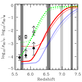
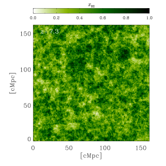
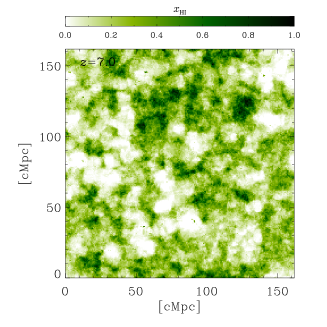
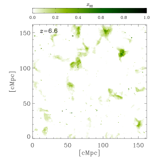
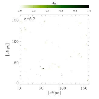
The ionizing source model obtained from the RHD simulation (§2.1 and in eq. [3]) may have uncertainty especially in the escape fraction of ionizing photons, because the escape fraction is known to depend on the spatial resolution of numerical simulations (e.g., Wise et al. (2014); Kimm et al. (2017); Sumida et al. (2018)). Therefore, we also carried out two additional reionization simulations, where the Lyman continuum spectra were changed to be a 1.5 times higher or lower photon production rates. Hereafter, we refer to the high emissivity, fiducial, and low emissivity models as , , and reionization models, respectively. The simulated reionization histories are shown in Fig. 1. These three models fully agree with the latest Thomson scattering optical depth measurement by the Planck satellite (Planck Collaboration, 2016b): , , and for the , and models, respectively, against the observation . For the model, H i distributions in the widths of some HSC narrowband filters are found in Fig. 2.
3 LAE model
The cosmological Ly radiative transfer can be divided into three components: the production in a galaxy, the transfer in the galaxy (including its ISM and CGM [or halo]) and the transfer in the IGM (e.g., McQuinn et al. (2007); Meiksin (2009); Laursen et al. (2011); Jensen et al. (2013); Kakiichi et al. (2016)). The observable flux of the Ly line can then be expressed as
| (4) |
where is the Ly luminosity produced in a galaxy, is the Ly escape fraction in the ISM (and halo) of the galaxy, is the IGM transmission for Ly photons, and is the luminosity distance toward the galaxy. In the following subsections (§3.1, 3.3 and 3.4), we will describe how we model and calculate the three quantities related to Ly. In §3.2, we will present an Ly line profile modeling.
Another important quantity, the source rest-frame equivalent width of the Ly line, is defined as
| (5) |
where is the continuum flux density at the Ly wavelength , is that at the UV wavelength , and is the UV spectral slope (). We will also describe modeling of the UV continuum in a later subsection (§3.5).
3.1 Ly production in a galaxy
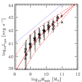
We make a simple recipe of the Ly photon production rate as a function of halo mass from the RHD galaxy formation simulation in §2.1 by Hasegawa et al. (in prep.) Fig. 3 shows the total (recombinationcollisional excitation) luminosity of Ly photons of galaxies at –7 in the simulation. The solid line on the figure is our recipe described as
| (6) |
where is the total intrinsic Ly luminosity normalized by erg s-1, is the halo mass normalized by M⊙, and accounts for the fluctuation of the Ly production. We draw a Gaussian random number with the mean of zero and the standard deviation of for , where
| (7) |
for , otherwise . The dashed lines in Fig. 3 show the range around the fiducial equation (6). The fluctuation in Ly production may account for a different star formation history of each halo. Jensen et al. (2013, 2014) adopted a similar log-normal fluctuation but their dispersion was 0.4-dex as a constant.
Since the dispersion described in equation (7) is somewhat large, an abnormally large Ly luminosity may happen in case without any limit. Therefore, we set an upper limit of the Ly luminosity indicated by the dotted line in Fig. 3 as . This choice is arbitrary but the RHD simulation results may suggest an upper limit around there.777 The distribution of the Ly production rate at a certain halo mass in the RHD simulation does not follow a Gaussian function but a function with an upper truncation. In reality, a finite time-scale of star-formation sets an upper limit on the star-formation rate in a halo, and then, the Ly production rate. In practice, when we obtained a Ly luminosity over the limit in a Monte Carlo trial computing the fluctuation and the luminosity , we discard it and draw another random number.
The simulated Ly luminosity shown in Fig. 3, i.e. our recipe described in equation (6), already includes the effect of the ionizing photon escape which reduces the Ly photon production rate. The exponential part in equation (6) accounts for this effect in lower halo mass where the ionizing photon escape becomes more significant (typically % for M⊙; Hasegawa et al. in prep.). However, the halo mass of the observed LAEs is larger than, say, M⊙ as found in §5.1 and the ionizing photon escape is not very large for these halos (typically % or less).
3.2 Ly line profile through the ISM
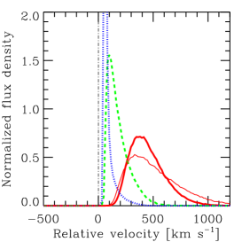
The Ly line profile is modulated by multiple resonant scatterings during the transfer in the ISM (e.g., Verhamme et al. (2008); Yajima et al. (2012, 2015)). Depending on the line profile, the IGM transmission is also changed (e.g., Yajima et al. (2017)). When the gas in the ISM is outflowing, the line profile shows an asymmetric shape with a red wing (e.g., Dijkstra et al. (2006)), resulting in a higher transmission through the IGM in the Hubble flow. Recent observations indicated that a large fraction of high-redshift LAEs have outflowing gas (e.g., Ouchi et al. (2010); Yamada et al. (2012); Shibuya et al. (2014)). In this work, for the simplicity, we consider line profiles through spherically uniform outflowing gas with the velocity structure of
| (8) |
where is the radius of the gas distribution and is the outflow velocity at . We set kpc, while the line profile does not depend on but only on the H i column density of the gas distribution and . We calculated the transfer of photon packets in 100 expanding spherical shells by using a Monte Carlo method (Yajima et al., 2012, 2014, 2017). Fig. 4 shows examples of line profiles. We find a significant H i column density dependence but the dependence is small. In the following sections, we consider the cases with , 19, or 20 and a fixed which is typically observed in LAEs (e.g., Hashimoto et al. (2013))
3.3 Ly escape fraction from a halo
The transfer of Ly photons in a galaxy is a complex process because of resonant scattering by neutral hydrogen. Numerical simulations show a large dispersion of the Ly escape fraction for fixed galaxy properties (e.g., Yajima et al. (2014)). We try to model this stochasticity, assuming a simple Gaussian function where both of the mean and the dispersion are equal to :
| (9) |
A possible explanation for this treatment is found in Appendix 1.
The mean Ly optical depth, , for a halo with the mass of can be described as
| (10) |
where the pivot value, , at the halo mass of M⊙ is a model parameter and the index describes the halo mass dependence of . Here we consider two cases of (no halo mass dependence) and corresponding to a case of where the right-hand-side means a column density and is the virial radius of a halo (). A similar halo mass dependence of the case is observed in numerical simulations (Yajima et al., 2014). Finally, the escape fraction of Ly photons is given by
| (11) |
with drawn from the probability distribution of equation (9).
As found in the subsequent sections (see table 1), –5. For such a small , we easily obtain an unphysical negative under the Gaussian probability distribution of equation (9). We just discard it and redraw another . This treatment gives modulation to the Gaussian function of equation (9).
3.4 Ly transmission through the IGM
The IGM transmission of the Ly line is defined as
| (12) |
where is the Ly line profile as a function of the wavelength, , in the source rest-frame and is the IGM optical depth at . The line profile is one observable at the virial radius of the halo of interest described in §3.2.
The IGM optical depth against Ly photons along a physical length coordinate, , defined from an object to an observer is
| (13) |
where is the neutral hydrogen cross section for Ly photons, is the wavelength in the gas rest-frame, is the temperature of gas, and is the number density of neutral hydrogen. The gas rest-frame wavelength is and , where is the Hubble parameter at redshift . We have neglected any peculiar motion of gas. We fix in a simulation box with its redshift . We define the IGM to be gas out of halos in this paper. Then, the integral starts at the virial radius, , of the halo of interest. The upper limit of the integral, , is arbitrary but several tens of comoving Mpc is sufficient for convergence.
The Ly cross section of neutral hydrogen is given by
| (14) |
where is the Voigt function with being , and . The light speed in vacuum is cm s-1, the Ly frequency Hz and the natural broadening width in frequency Hz corresponding to the Einstein coefficient of Hz. The thermal Doppler width in frequency , where with the Boltzmann constant erg K-1 and the proton mass g. The Voigt function is calculated by using the analytic approximation of Tepper-Garcia (2006).
For each simulation box, we set 6 directions (, , ) for lines-of-sight and calculate of each halo. We have confirmed as a sanity check that the 6 directions’ transmissions averaged over a number of halos agree with each other and the difference is at most %.
3.5 UV continuum
We assume a simple linear relation between UV luminosity and halo mass, which is consistent with the prediction of a cosmological hydrodynamical simulation by Shimizu et al. (2014)888In Shimizu et al. (2014), they have derived a power-law relation of in their eq. (9) from a fit for all the simulated galaxies, whereas the linear relation and dispersion in this paper are obtained from a fit for their data binned along shown in their Fig. 5.:
| (15) |
where brings fluctuation in the UV magnitude. We draw a Gaussian random number with the mean of zero and the standard deviation of for , where
| (16) |
for , otherwise . This is also obtained from the Shimizu et al. (2014) simulation results. We here note that the fluctuation of the UV magnitude and that of the Ly production rate are not correlated in our modeling, while they are probably correlated in reality. Fortunately, we will find that the UV magnitude fluctuation is small and has a relatively small impact and that the fluctuation of the Ly production is less important than that of the Ly optical depth. Therefore, this point does not affect the conclusions of this paper.
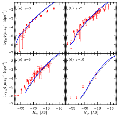
Fig. 5 shows a comparison with observations in UV LFs at , 7, 8, and 10. We find a reasonable agreement although there are overpredictions at the faint-end, especially at , and underpredictions at the bright-end at . This is probably caused by our simple linear assumption in the halo mass and UV magnitude relation (eq. 15). Indeed, a non-linear relation between halo mass and UV magnitude is observed in LBGs at (Harikane et al., 2016, 2018a). Given the reasonable agreement of our simple model and UV LFs at and 7 in the range of , the non-linearity effect would be small in our study.
We also assume an empirical relation between and the UV spectral slope , where the UV flux density per unit wavelength interval , reported by Bouwens et al. (2014):
| (17) |
where again accounts for fluctuation in . This may be caused by differences of the star formation history and the dust content of each halo. We draw a Gaussian random number with the mean of zero and the standard deviation of which is obtained from the simulation of Shimizu et al. (2014) and consistent with the random errors estimated in Bouwens et al. (2014). We do not account for the systematic errors reported in Bouwens et al. (2014) to avoid an abnormally large dispersion in at low luminosity and it should be reasonable because the value in equation (17) agrees with the prediction by Shimizu et al. (2014).
3.6 Virtual observations
To make the models as realistic as possible, we have made virtual observations of the simulation box. First we randomly select the observation direction among six directions along the axes (i.e. , and ) and select a random point in the box as the point (0,0,), where is the radial comoving distance toward the redshift of the simulation output. Then we obtain redshifts of all halos from their coordinates along the selected observation direction and map the halos into the celestial sphere by using the other two coordinates and the redshift of them. We then calculate the model observed magnitudes of the halos through Subaru HSC broadband and narrowband filters. Photometric errors are also taken into account according to the limiting magnitudes of observations by Konno et al. (2018) for and and by Konno et al. (2014) for . Using these predicted apparent magnitudes, we can select mock LAEs by the same magnitude and color criteria as the real observations (e.g., Shibuya et al. (2018a)). Note that unlike the real observations, there is no contamination of low- objects in the mock LAEs because we do not make a light-cone from a series of the simulation outputs but treat only a single simulation output for each redshift of interest in the virtual observations (but we have considered the redshift difference within the simulation box). Our simulation box has a deg2 area for , while the early SILVERRUSH data have 14 deg2 for LAEs and 21 deg2 for LAEs (Shibuya et al., 2018a). Since the NB widths correspond to about 1/4 of the simulation box size in the comoving scale, we may obtain at least 4 different slices of the NB survey from a simulation output. The -axes can produce different slices, resulting in 12 sets. On the other hand, the stochastic processes in the LAE modeling described in the previous subsections produce mock LAEs from different halos in different trials. This may allow us to have a much larger number of different sets of mock LAEs from a single simulation output (i.e. a single distribution of halos). We then repeat to produce mock LAE catalogs 100 times or up to 500 times, respectively, for LFs and LAE fractions or for ACFs. This may be equivalent to a set of observations of 100–500 patches of 1 deg2 area in the sky.
3.7 Models and parameter calibration
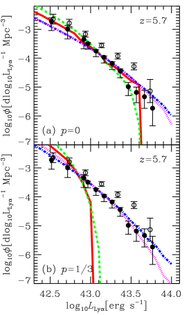
In this paper, we consider models depending on the presence of dispersion of the Ly production in a halo (eq. 7), stochasticity of the Ly optical depth in the halo (eq. 9), and halo mass dependence of the Ly optical depth (eq. 10). These 8 models are named as A to H and listed in Table 3.7. There is only a single free parameter in these models: , a pivot value of the ISM Ly optical depth at a halo of M⊙ (see eq. 10). We determine the value for each model so as to reproduce the observed Ly LF at . Since the IGM is highly ionized and has only a minimum effect on the LFs at this redshift, the reionization history is not matter and we adopt the model for the calibration. We use the early data of SILVERRUSH (Konno et al., 2018) as the reference observations. As we discuss in Appendix 2, their LFs are corrected for incompleteness and the filter transmission effects and then considered to be the best estimates of the true LFs. Therefore, we compare theirs with the true LFs in our simulation box. Fig. 6 shows the results of the parameter calibration from this comparison. In fact, models E and F can not reproduce the observed LF at all. The obtained pivot values are listed in Table 3.7.
Santos et al. (2016) (and also Matthee et al. (2015)) presented significantly higher LFs than those of Konno et al. (2018) and other previous ones obtained with Subaru/Suprime-Cam (Shimasaku et al., 2006; Ouchi et al., 2008). Since the reason of this discrepancy is unclear, we also calibrated with the LF at by Santos et al. (2016). However, with this calibration, no model could reproduce the LAE fraction (§4.3), may suggesting a possible overestimation in their LFs.
List of the LAE models. Model Ly LF ACF LAE fraction A 0 — — 1.6 B 0 eq.(7) — 1.9 C 0 — eq.(9) 3.1 D 0 eq.(7) eq.(9) 4.6 E 1/3 — — 0.6 F 1/3 eq.(7) — 1.0 G 1/3 — eq.(9) 1.1 H 1/3 eq.(7) eq.(9) 2.4 {tabnote} Notation is as follows: good, marginal, and bad.
3.7.1 Models without halo mass dependence of the Ly optical depth in the halo ()
In the following, we present brief comments on each models. The first four models (A–D) have no halo mass dependence of the Ly optical depth, namely in equation (10).
Model A
This case has neither dispersion of the Ly production nor that of the halo Ly optical depth. Thus, this model is the simplest case with a constant Ly luminosity per halo mass and a constant Ly escape fraction for all halos, which is often found in the literature (e.g., McQuinn et al. (2007); Iliev et al. (2008); Jensen et al. (2013, 2014); Kakiichi et al. (2016); Kubota et al. (2017); Yoshiura et al. (2018)). This model is shown as the solid line in Fig. 6 (a). The adopted constant escape fraction of Ly photons is 0.20. The observed LFs are reproduced reasonably well although a sudden dearth of the model LAEs at erg s-1 apparently seems inconsistent with the data.
Model B
This model has dispersion of the Ly production but not that of the halo Ly optical depth. This case also assumes a constant Ly escape fraction for all halos. This model is shown as the dashed line in Fig. 6 (a). Relative to Model A, Model B predicts a steeper LF. This is due to the dispersion of the Ly production and the upper limit on the Ly emissivity (see Fig. 3). In fact, the dispersion itself makes the LF shallower than Model A (see also Jensen et al. (2014)), especially at the faint-end erg s-1 in our case. On the other hand, the luminosity upper limit in the current model setup makes the distribution of the Ly luminosity asymmetric with a cut-off in the luminous side. This causes the steeper slope in the luminous-end than Model A. The constant Ly escape fraction is 0.15 smaller than that of Model A in order to fit the observed LF.
Model C
This case has no dispersion of the Ly production but does have dispersion of the halo Ly optical depth. Therefore, a stochastic Ly escape from a halo is realized. This model is shown as the dot-dashed line in Fig. 6 (a). The LF becomes shallower than Model A because of the dispersion of the halo Ly optical depth. There is a more chance to have a large escape fraction than a small one because of asymmetry of an exponential function of the escape fraction in eq. (11) even under a symmetric Gaussian probability distribution of the optical depth described in §3.3, leading to more LAEs in luminous bins. To fit the observed LF, an average Ly escape fraction is as small as 0.045.
Model D
This model has both dispersions of the Ly production and the halo Ly optical depth. This case is shown as the dotted line in Fig. 6 (a) and is very similar to Model C with slightly less LAEs in luminous bins caused by the upper limit of the Ly production. The smallest average Ly escape fraction of 0.010 is required to fit the observed LF.
3.7.2 Models with halo mass dependence of the Ly optical depth in the halo ()
The rest four models (E–H) have a halo mass dependence of the halo Ly optical depth, that is in equation (10). This dependence comes from the assumption that the optical depth is proportional to the matter column density in a halo (see a discussion below eq. 10). In these cases, the values of the pivot optical depth at a halo of M⊙ tend to be smaller than those in the models with . This is natural because a more massive halo has a larger optical depth. An average optical depth over all halos would be equivalent.
Model E
This model has neither of the dispersions like Model A. The LF is shown as the solid line in Fig. 6 (b). Due to higher Ly optical depths in more massive halos, the LF becomes too steep and totally inconsistent with the data.
Model F
This model has only the dispersion in the Ly production like Model B. The LF is shown as the dashed line in Fig. 6 (b). Due to the dispersion of the Ly production with an upper limit, the LF becomes further steeper than Model E and again totally inconsistent with the data.
Model G
This case has only the dispersion in the halo Ly optical depth like Model C. The LF is shown as the dot-dashed line in Fig. 6 (b) and becomes much shallower than Models E and F due to the dispersion of the Ly optical depth. As a result, the LF is reasonably consistent with the data.
Model H
This case has both of the dispersions like Model D. The LF is shown as the dotted line in Fig. 6 (b) and is similar to Model G but slightly steeper due to the dispersion of the Ly production with an upper limit.
4 Results
We are ready to compare our LAE models with the observations, in particular, the early results of SILVERRUSH (Ouchi et al. (2018); Konno et al. (2018)). Comparing the models to the LAE luminosity functions (LFs; Konno et al. (2018)), the angular correlation functions (ACFs; Ouchi et al. (2018)), and the LAE fraction as a function of the UV magnitude (Ono et al. (2012)), we will select the best model in this paper.
4.1 Ly luminosity function
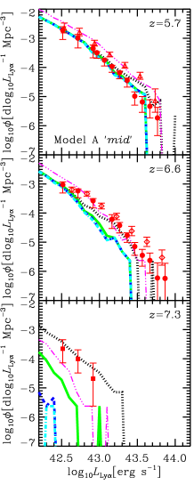
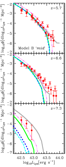
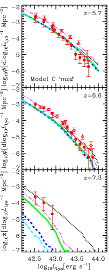
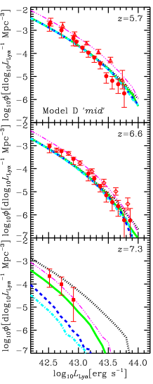
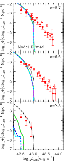
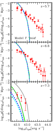
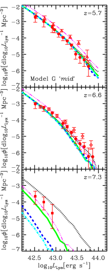
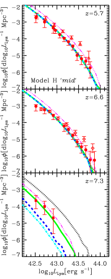
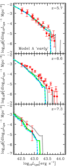
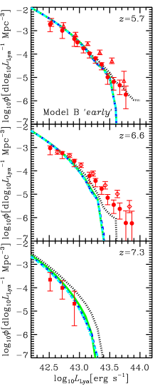
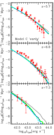
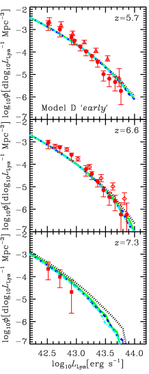
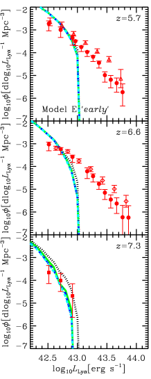
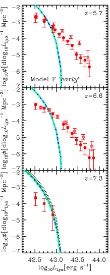
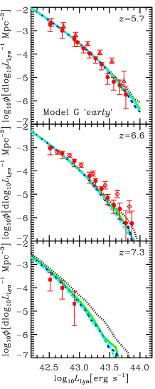
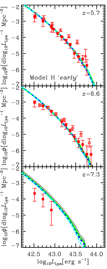
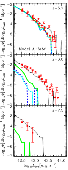
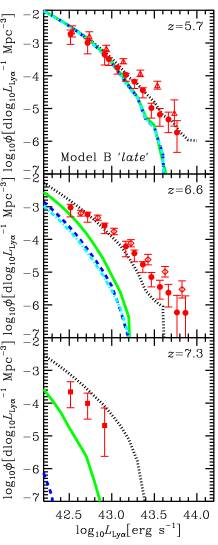
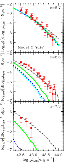
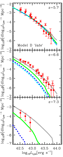
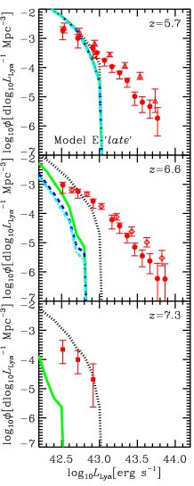
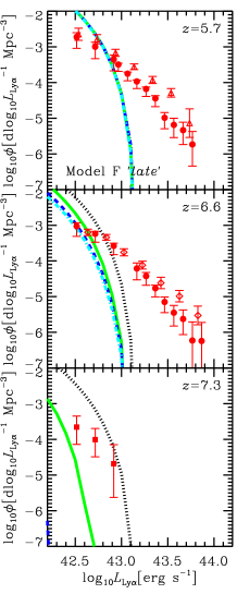
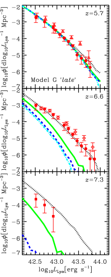
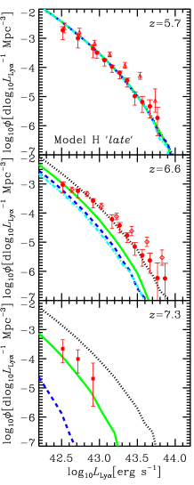
We compare the true LFs in our simulation box with the SILVERRUSH early LFs of Konno et al. (2018) directly because the observed LFs are already corrected for incompleteness and the filter transmission effects (see Appendix 2). Figs. 7, 8 and 9 show the comparisons of the observed LFs with the models for the , and reionization histories, respectively. The dotted (black) lines are the model LFs without the IGM transmission, namely those through a completely ionized IGM. Thus, these put the upper limit of the LAE number densities in each model. If the dotted line in a panel becomes far below the observed data, the model should be rejected. Such cases are the models E and F which predict too few LAEs brighter than erg s-1. The models A and B are marginal due to a small number densities of LAEs at erg s-1 and at . Other models are qualified.
The solid (green), dashed (blue) and dot-dashed (cyan) lines, which are overlapped each other in many cases, are the model LFs through the IGM transmission with different Ly line profiles depending on the H i column density in the outflowing gas. As found in Fig. 4, the velocity shift of the line peak becomes larger for a larger column density, resulting in higher IGM transmission. This effect becomes more pronounced in the IGM with a higher . For example, in the reionization model (Fig. 7), the difference is visible only at . On the other hand, in the model (Fig. 8), the difference is small even at , whereas it can be found also at in the model (Fig. 9). At , the difference is negligible no matter which reionization model.
Regarding the IGM transmitted LFs (colored lines), the qualified models (C, D, G and H) including marginal ones (A and B) show an excellent agreement between the predictions and the observed data at where we have calibrated these models with the reionization history. At , Models C and G (and also A and B) in the and histories predict less LAEs than observed, while Models C and G in the history still agree to the data. The same thing is found at . On the other hand, Models D and H in the and histories are consistent with the data at and 7.3 (Model H in the history seems overprediction at ). However, these models in the history also underpredict the LAE number densities at . At , these models are still touching the lower bound of the measurements. Overall, the observed Ly LFs at and seem to favor more ionized IGM like the history. This point will be discussed more in §5.2.
In Fig. 7, we also show the LFs calibrated with Santos et al. (2016) instead of Konno et al. (2018).999We just use the same pivot values, , for the models E and F in the both calibrations because the LF shape is inconsistent with the observations. The results are qualitatively similar to those with Konno et al. (2018). The predictions at are smaller than the observed LFs (open symbols) of Matthee et al. (2015) updated by Santos et al. (2016) in the bright-end. This again indicates somewhat earlier reionization than the history.
4.2 Angular correlation function
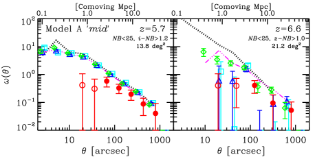
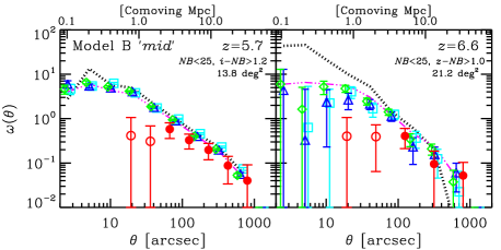
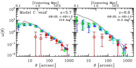
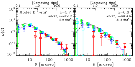
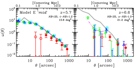
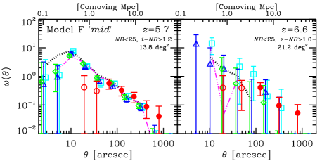
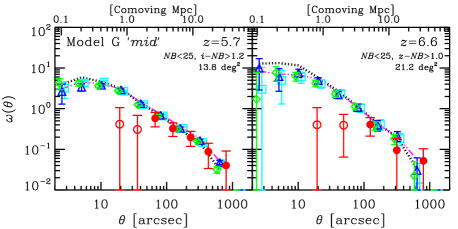
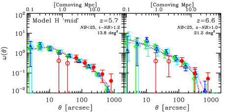
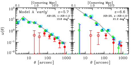
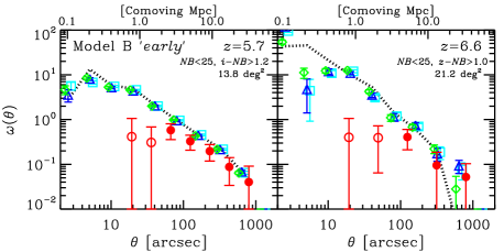
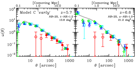
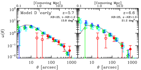
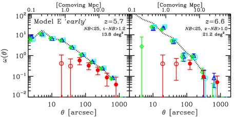
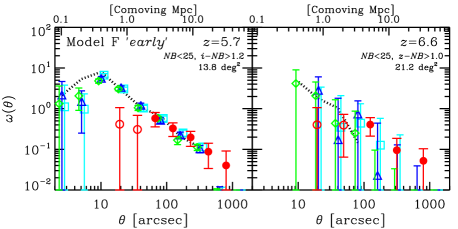
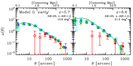
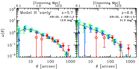
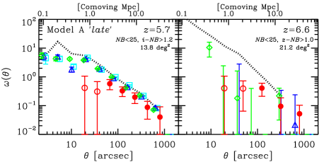
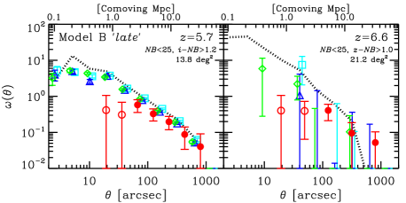
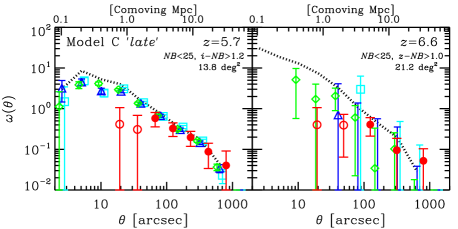
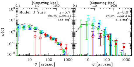
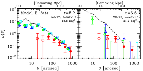
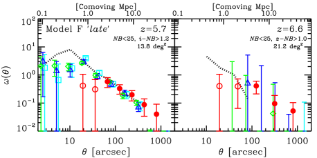
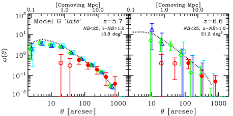
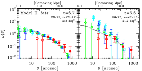
We compare the model ACFs with the SILVERRUSH early results by Ouchi et al. (2018). The model ACFs are calculated by the same way as Ouchi et al. (2018); we select mock LAEs by the same color-magnitude criteria via virtual observations (§3.6), count the numbers of pairs of LAE–LAE, LAE–random position, and random–random positions, and estimate the ACFs according to Landy & Szalay (1993). The virtual observations are repeated 300- and 500-times to secure sufficiently large mock LAE catalogs for and , respectively. Figs. 10, 11 and 12 show the comparisons at and 6.6 for the , and reionization histories, respectively. The areas of the current SILVERRUSH also noted in the panels are used to scale the model error-bars. However, the model error-bars are probably underestimated because we account only for Poisson errors. The effect of the cosmic variance can be estimated by a Jackknife method observationally from ACFs of Ouchi et al. (2018). We have found that for a survey area of 20 deg2 as the combination of the Poisson errors and the cosmic variance. Since the Poisson errors are much smaller than this and the cosmic variance is the dominant source of uncertainties for the current SILVERRUSH results.
The dotted (black) lines show the model ACFs through the completely ionized IGM (i.e. no IGM effect). In these cases, the numbers of the mock LAEs are the largest in each model and the ACFs up to about 1000 arcsec are derived successfully as the observations have done, except for Model F at , where the number of bright LAEs satisfying the NB magnitude criterion is limited and we could derive the ACF only arcsec. Therefore, Model F is disqualified here.
The diamonds (green), triangles (blue) and squares (cyan) with error-bars are the model ACFs through the IGM transmission depending on the different H i column density for the line profile. At , the model ACFs are almost overlapped on the dotted (black) lines (i.e. the fully-ionized IGM) irrespective of the models and the reionization histories because of the high ionization degree at the redshift in our simulations. Each model predicts a different correlation amplitude. Comparing with the observed data at , Models C, D, G and H are very consistent with the data within the error-bars in the angular separation between 60 and 1000 arcsec, while Models A, B and E seems marginally overpredict the amplitude.
At a smaller angular separation ( arcsec), the observed amplitudes are smaller than the models which continue to increase up to arcsec. Since we do not identify sub-halos in a halo (§2.1), the models do not include the correlation within a single halo, so-called one halo term. But this becomes important only at arcsec. Therefore, the increase of the model ACF at 10–60 arcsec is caused by a different thing. This is probably the non-linear halo bias effect (Reed et al., 2009; Jose et al., 2016, 2017). Jose et al. (2017) argue that a model with the non-linear effect can better reproduce the LBG ACFs obtained from the Canada-France-Hawaii Telescope Legacy Survey data (Hildebrandt et al., 2009). Recently, Harikane et al. (2018a) has also found this feature in the LBG ACFs from the Subaru/HSC survey called GOLDRUSH (Ono et al., 2018) thanks to a huge number of the sample (). If the number of the LAE sample increases in future, a similar non-linear effect may be found in the observed LAE ACFs as predicted by the models.
At , the difference due to the IGM ionization degree appears, especially in the reionization history. The largest impact is the decrease of the numbers of the mock LAEs. As a result, we have failed to obtain the ACFs, for example, in Models A, E and F of the history, in Model F of the history, and many models in the history. Since the observations provide us with the firm ACF measurements even at , the history is disfavored. For the and histories, Models B, C, D, G, and H are consistent with the observations between 100 and 1000 arcsec. At a smaller angular scale, the model ACFs are again higher than the observations.
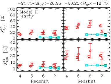
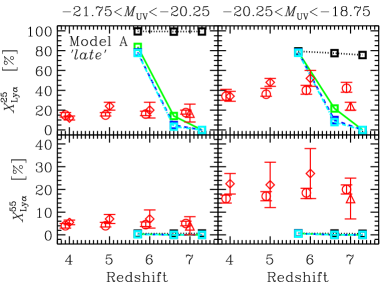
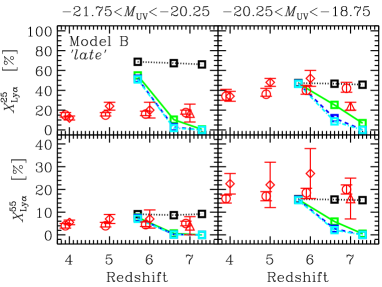
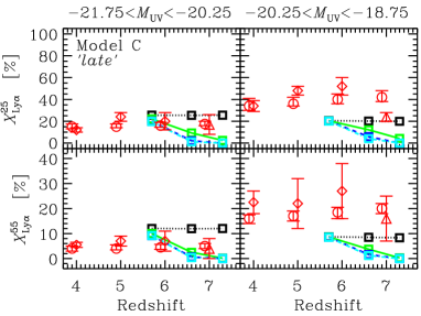
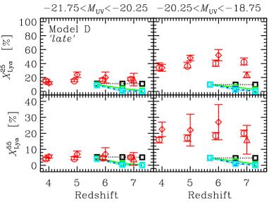
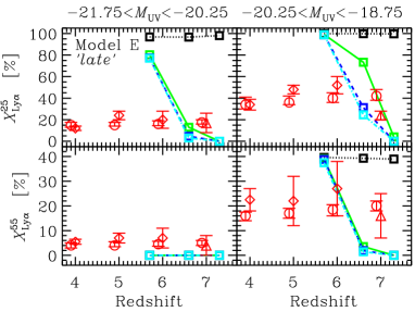
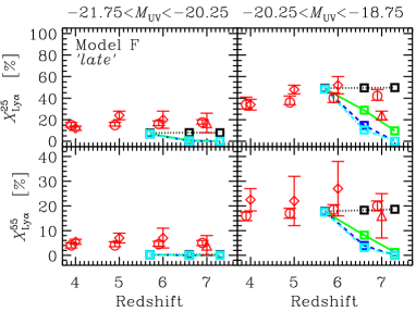
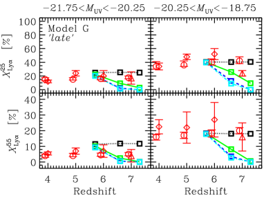
4.3 LAE fraction in LBGs
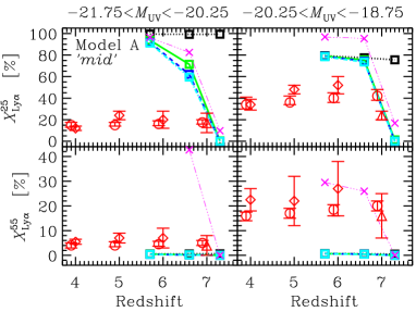
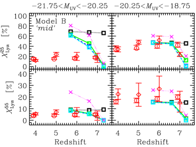
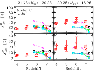
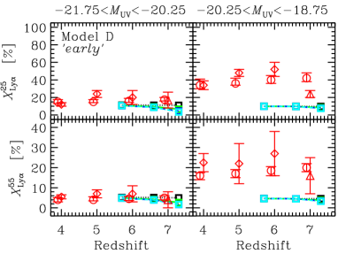
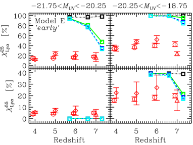
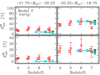
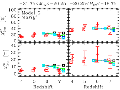
We compare the observed LAE fractions in LBGs with those predicted by our models. Since the observational LAE fractions were usually obtained from spectroscopy, their EWs can be regarded as true ones (i.e. not-estimated by NB photometry). Therefore, we will use the true EWs in our models. However, there might be systematic bias in the observed data because only a small number of LBGs has been targeted and the Ly fraction is sensitive to the inhomogeneity of the spectroscopic detection limit (e.g., Ono et al. (2012)).
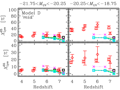
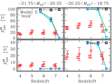
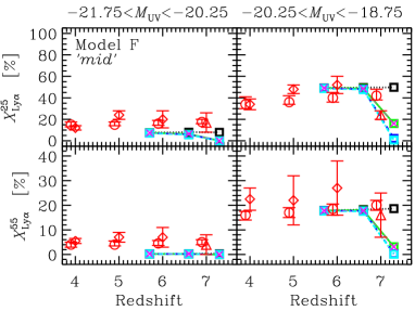
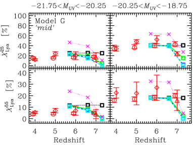
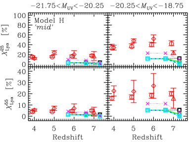
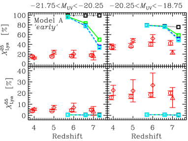
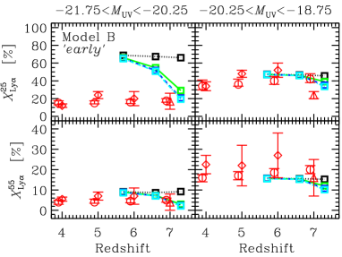
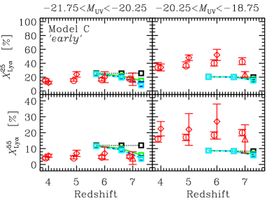
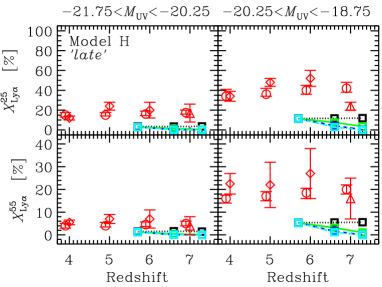
Figs. 13, 14 and 15 show the comparisons of the observed LAE fraction in LBGs with the models for the , and reionization histories, respectively. For each model, there are four sets: the smaller or larger threshold of the Ly equivalent width (EW) and the brighter or fainter UV luminosity range. We have found that this comparison is the most critical one. Only Model G shows a reasonable agreement with all four sets. Model B is the second best because it reproduces the three sets but it fails in the lower EW and the brighter UV. Models C and D reproduce the two brighter UV sets. However, they significantly underpredict the LAE fraction in the fainter UV galaxies because there is no halo mass (or UV luminosity in our model) dependence of the Ly optical depth which is a key ingredient to reproduce a higher LAE fraction in a fainter galaxy sample. Models E and F can reproduce one or two sets in the fainter sample but not in the brighter sample. Models A and H fail in all four sets.
It is interesting to look into the reason why Models A and H fail. Model A has no stochastic process in Ly production and Ly transmission in a halo but does have in UV luminosity and slope. Neglecting the latter effect, we obtain the rest-frame EW Å for and with . As a result, % UV bright galaxies satisfy EW Å in an ionized Universe (i.e. ), but there is no LAEs with EW Å. The halos with corresponding to are affected by the stochastic processes in UV luminosity and slope and the EWs fluctuate, resulting in an LAE fraction in the UV fainter samples. Model H, on the other hand, has all stochastic processes. Due to the fluctuation in Ly production, less massive halos have a significant chance to get a bright Ly luminosity. Since they are numerous, a larger pivot value of the Ly optical depth in a halo is required to keep the Ly LF consistent with the observations. Model H also has a halo mass dependency in the Ly optical depth, extinguishing Ly in more massive halos. The halo mass is directly connected to the UV luminosity in our modeling. As a result, a dearth of LAEs in massive halos bright in UV emerges, which is inconsistent with the observations.
The effect of the reionization (or IGM neutrality) can be found in Figs. 13, 14 and 15. For example, in the history (Fig. 13), we can find significant decrements of the LAE fraction at where (see Fig. 1) and even at () in some cases. In the history (Fig. 15), the LAE fraction decrements are significant already at (). Even in the history (Fig. 14), the decrements can be found at () and also at () in few cases. Therefore, the reionization signature is indeed imprinted in the redshift evolution of the LAE fraction (Stark et al., 2010, 2011; Ono et al., 2012) and the decrements become significant when . This point will be discussed again in §5.2.
In Fig. 13, we also show the LAE fractions in the LF calibration with Santos et al. (2016). Unlike the calibration with Konno et al. (2018), we can not find any model reproducing all four sets of the LAE fraction evolution. In the Santos et al. (2016) calibration, the LAE fractions are often overestimated, indicating possible overestimation of their LF.
5 Discussion
From the comparisons in the previous section, we have identified Model G as the best model in this paper (Table 1). In this section, we will discuss the physical properties of the LAEs in Model G (§5.1) and implications how to discuss cosmic reionization with LAEs (§5.2).
5.1 Nature of LAEs in the reionization epoch
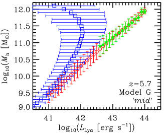
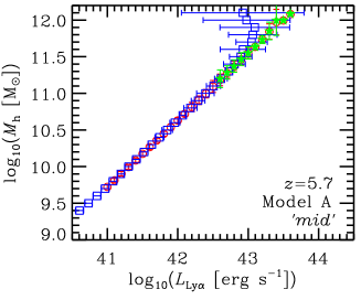
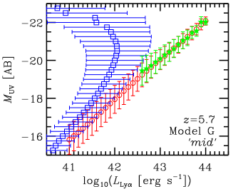
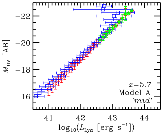
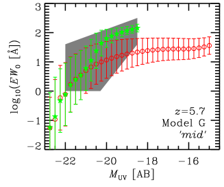
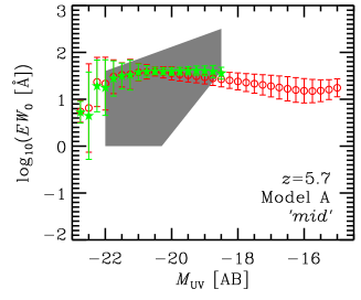
Fig. 16 shows some physical properties of galaxies predicted from the best-model, Model G. We also show the predictions from the simplest model, Model A, as a reference. The top panels show the predicted relations between halo mass, , and observable Ly luminosity, . The circles and error-bars (red) represent the average and its standard deviation of the halos having a within a 0.1-dex range around the value of the horizontal axis. The squares and error-bars (blue), on the other hand, represent the average and its standard deviation of the halos having a within a 0.1-dex range around the value of the vertical axis. For Model A, the circles and squares are completely overlapped, except for erg s-1 and M⊙ because of the one-to-one correspondence of and in the model without any stochastic process. The deviation for the massive or luminous halos is caused by a fluctuation of the IGM transmission. In our reionization simulation, the neutral fraction around massive halos tends to be higher and the transmission varies significantly, whereas that around less massive halos tends to be lower and the transmission keeps high (Hasegawa et al. in prep.).
Interestingly, Model G is very different from Model A. In Model G, luminous LAEs ( erg s-1) tend to have a massive halo mass ( M⊙) as shown by the circles. However, such a massive halo on average has much smaller Ly luminosity (see the squares) and only a small fraction of these massive halos is observed as luminous LAEs. This is very consistent with a duty cycle hypothesis of the LAE population (e.g., Ouchi et al. (2010, 2018)). The middle panels of Fig. 16 show correlations between the UV magnitude, , and and indicate a very similar thing. According to the LAE fraction in UV luminous halos (Figs. 13, 14 and 15), the LAE fraction is 5–20% depending on the equivalent width () criterion at .
The five-pointed stars with error-bars (green) are the same as the circles but for the halos which would be selected as LAEs by real observations (Shibuya et al., 2018a). We set the NB limiting magnitude corresponding to erg s-1. We have found a typical halo mass of M⊙ which excellently agrees with that estimated by Ouchi et al. (2018) through the clustering analysis. This is a natural consequence because we have reproduced the observed ACFs of Ouchi et al. (2018) in §4.2.
The bottom panels of Fig. 16 show the relation between the UV magnitude, , and the Ly equivalent width in the source rest-frame, . The shaded area is the observed range in the diagram (Furusawa et al., 2016). There is an observational trend that UV bright galaxies have a smaller , so-called “Ando relation” (Ando et al., 2006, 2007). Note that the sample galaxies for the observation of Furusawa et al. (2016) are mainly NB-selected LAEs and a comparison with our models is fair. We have applied the same limit as the observation to the color-magnitude selected halos in the model (five-pointed stars). The offset between the five-pointed stars and the circles in Model G is caused by the NB excess selection in the mock observation. In Model G, there are some NB-selected “LAEs” with Å at . These halos were selected by a Lyman break mimicking an NB excess. However, the number fraction of such bright NB-selected halos among the NB-selected halos of is as small as 3%. The best-model, Model G, excellently reproduces the Ando relation although the simplest, Model A, does not. The origin of the Ando relation in Model G is the halo mass dependence of the Ly optical depth. Therefore, the Ando relation can be understood as a consequence from a simple scaling of halo mass: more H i in more massive halos.
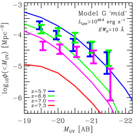
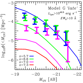
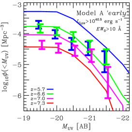
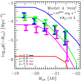
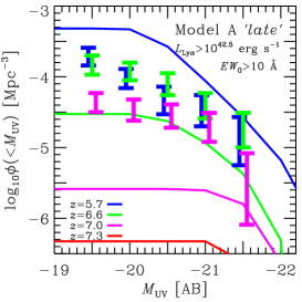
Fig. 17 shows the UV luminosity functions for LAEs at , , and . The observational data are taken from Ota et al. (2017) and references therein. We show the best-model, Model G, and the simplest model, Model A as a comparison. Both models agree with the observations in some cases but do not in other cases. The or reionization histories show better agreement than the cases. However, the observed little evolution between and is not consistent with the models which predict a significant evolution. The physical reason of this disagreement is unclear. On the other hand, we have found that the model UV luminosity function is sensitive to the selection criteria for the LAEs. In this comparisons, we have adopted a set of Ly luminosity and equivalent width cuts similar to those in Ota et al. (2017). If we change the Ly luminosity limit, however, the UV LF easily moves vertically. Therefore, we need to be careful in the Ly luminosity limit in such comparisons in future.
5.2 To derive the reionization history with LAEs
5.2.1 Ly luminosity function and density
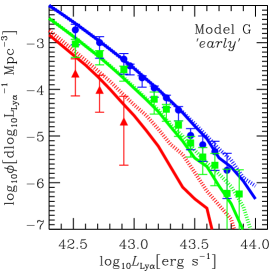
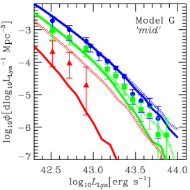
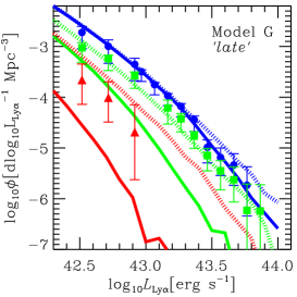
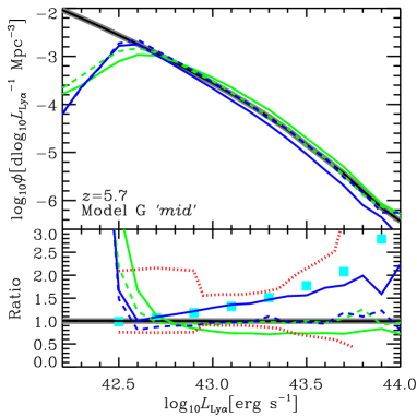
Fig. 18 shows the redshift evolution of the Ly LFs and comparisons with the best-model, Model G. The three panels correspond to the , and reionization histories from left to right, respectively. The solid and dotted curves are the cases with/without the IGM Ly transfer effect, respectively. Namely, the dotted curves are the fully-ionized IGM cases. At , the models reproduce the observations very well independent of the reionization model because the neutral fraction is very low at the redshift in any model. On the other hand, the model predicts much fewer LAEs than the observations at and . The model also predicts somewhat fewer LAEs but the model expects a bit more LAEs at . Therefore, the real Universe may have evolved through a middle history of the and models.
In this way, we may derive the reionization history from the Ly LFs. Such attempts have been made in literature (e.g., Kashikawa et al. (2006); Ouchi et al. (2010); Kashikawa et al. (2011); Konno et al. (2014); Ota et al. (2017); Konno et al. (2018)). The most serious difficulty in this analyses, however, is the degeneracy between the evolution of the LAE population and the IGM neutrality. Some authors have assumed the evolution (or no evolution) in the LAE population estimated from the LAE UV LFs and other authors have used theoretical model predictions. We take the latter approach here. The advantage compared to the previous works is that the best-model, Model G, in this paper can reproduce all of the Ly LFs, ACFs, and LAE fractions very well. Therefore, the reliability of the model would be high.
We introduce a measure of the IGM neutral fraction: the decrement of the observed Ly luminosity density (LD) compared to the model predictions in a fully-ionized IGM. Namely,
| (18) |
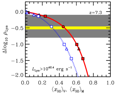
where is the integrated Ly LD. Fig. 19 shows these decrements obtained from Model G. We have found that these decrements at different redshifts and in different reionization histories can be described by the following single function of the neutral fraction, , excellently:
| (19) |
where is the decrement, , and is the volume-averaged or mass-averaged neutral fraction. The fitting parameters of , and are listed in Table 5.2.1 for a limiting Ly luminosity. In Table 5.2.1, we list the model predictions of the Ly LDs in a fully-ionized IGM, the observed Ly LDs, the decrements of the observed LDs and the estimated hydrogen neutral fractions. The observed decrements at are consistent with zero within uncertainties and we have obtained only upper limits of . At , the decrement is significantly negative, indicating a non-zero value of . The resultant values are and for the volume-averaged and mass-averaged , respectively. These at are consistent with the estimation by Konno et al. (2014) who assumed an evolution of the LAE population estimated from the LAE UV LFs and an analytic IGM transmission model by Santos (2004).
There is a precaution for using equation (19). These LD decrements are derived from the cases with a Ly line profile through an outflowing gas with its velocity km s-1 and H i column density . As we saw in Figs. 7, 8 and 9, the H i column density has an effect on the LF decrements. Therefore, if the typical H i column density in LAEs at the redshift interested is different from that assumed here, the fitting equation (19) will change. In addition, there may be systematic uncertainty in caused by the model calibration of LFs which we assume 0.1-dex (Table 5.2.1).
Fitting parameters of equation (19) for the case of . {tabnote} These parameters are derived from Model G assuming the Ly line profile through an outflowing gas with km s-1 and .
A summary of the estimations of the hydrogen neutral fraction.
†
†
References‡
5.7
(1)
6.6
(1)
7.0
(2)
7.3
(3)
{tabnote}
† The unit of the luminosity density is
erg s-1 Mpc-3. The lower limit of the luminosity in
integration is .
We assume 0.1-dex systematic uncertainty of the model calibration.
The references of the observed luminosity densities. The
numbers correspond to the following references: (1) Konno et al. (2017),
(2) Ota et al. (2017), (3) Konno et al. (2014).
5.2.2 Other methods
The LAE ACFs are suggested to be useful to constrain the reionization history as well as the reionization topology (e.g., McQuinn et al. (2007)). On the other hand, our model predictions in Figs. 10, 11 and 12 do not show very clear differences in the ACFs between and . This is partly because is too small even at to make differences in ACFs. If we go to higher redshifts where is sufficiently large, however, the observable numbers of LAEs may be too small to obtain firm ACF measurements. Another reason may be the reionization topology in our simulation. This is basically “inside-out” as found in Fig. 2, but our simulation seems more modest than previous ones. The IGM Ly transmission at the redshift interested in this paper is actually lower for more massive halos. This is caused by two new features in our reionization simulation. One is that a smaller for more massive halos. The other is the spatially different clumping factor (Hasegawa et al. in prep. for more details). Therefore, the LAE ACFs may not be a useful probe of reionization as previously thought although further investigations in simulations are required.
The redshift evolution of the LAE fractions can be useful to derive the reionization history (e.g., Ono et al. (2012)). Our model predictions shown in Figs.13, 14 and 15 support this idea; the LAE fraction decrements become significant when . On the other hand, Oyarzún et al. (2017) raises a possibility that the drop of the LAE fraction is caused by survey incompleteness in . Future analyses are required to examine and correct the incompleteness effect.
The 21 cm–LAE cross-correlation is proposed to be another powerful tool to deduce the reionization history, especially the size of the ionized bubbles (e.g., Lidz et al. (2009); Kubota et al. (2017); Yoshiura et al. (2018)). So far, the LAE modeling remains rather simple assuming one-to-one correspondence between halo mass and Ly luminosity (e.g., Kubota et al. (2017)). Since we have shown its break down in this paper, adopting a better LAE model in such analyses will be an interesting future work.
6 Conclusion
We have presented new models of LAEs at , the reionization era, in a large-scale ( comoving Mpc3) radiative transfer simulation of reionization. Our LAE modeling is based on physically-motivated analytic equations, depending on the presence or absence of dispersion of Ly emissivity in a halo, dispersion of the Ly optical depth in the halo, , and the halo mass dependence of . We have critically examined the model with one-to-one correspondence between halo mass and Ly luminosity before transmission in the intergalactic medium (IGM), which is often adopted in previous studies. Comparing with the Ly luminosity function (LF) from the early data of the Subaru/HSC survey of LAEs called SILVERRUSH (Ouchi et al., 2018; Konno et al., 2018), we have calibrated the single adjustable parameter in our models: a typical Ly optical depth in a halo of M⊙. After comparisons of our models with Ly LFs at and , angular auto-correlation functions (ACFs) of LAEs at and , LAE fractions in Lyman break galaxies (LBGs) at , we have identified the best model which successfully reproduces all these observations. Our main findings are as follows:
-
•
The Ly LFs and ACFs are reproduced by multiple models, but the LAE fraction is turned out the most critical test. The simplest model adopting one-to-one correspondence between halo mass and Ly luminosity (Model A) overpredicts (or underpredicts) the number fraction of LAEs with (or ) among LBGs. Therefore, this model which many previous studies adopted has been ruled out.
-
•
The dispersion of and the halo mass dependence of are essential to explain all observations reasonably. However, a large dispersion of Ly emissivity assumed in this paper reduces a typical halo mass of LAEs too much and underpredicts the LAE fractions in LBGs with . Therefore, the Ly emissivity dispersion among halos may be small if it exists.
-
•
Based on the best model in this paper (Model G), we have discussed the physical properties of LAEs at . A typical halo mass of the LAEs is estimated at M⊙. The so-called “Ando-relation” is also reproduced and its physical origin is a simple scaling of halo mass: more H i in more massive halos.
-
•
We have presented a simple formula to estimate the intergalactic neutral hydrogen fraction, , from the observed Ly luminosity density at . While at , , and are still consistent with zero within uncertainties and the obtained upper limits are () as a volume-average, we have obtained a non-zero value of as a volume-average at .
Finally, we note a possible direction for future updates of the model. The best model, Model G, is characterized by the significant fluctuation in the halo Ly optical depth (or the Ly escape fraction) and the halo mass dependence on the optical depth. However, it may be puzzling that Model G has less importance of the fluctuation in the Ly production which is predicted by the radiation hydrodynamics (RHD) simulations (see Fig. 3). In this respect, our simple analytic treatment may be insufficient. Therefore, we will examine a new modeling of the halo Ly luminosity by using Ly transfer simulations in galaxies produced by the RHD simulations (Abe et al., 2018). The new recipe will include the production and transfer of Ly photons in halos as well as the line profile self-consistently. Such an updated LAE model will be compared with the full data set of SILVERRUSH (Ouchi et al., 2018) and CHORUS (Inoue et al. in prep.) in future.
The authors appreciate Taishi Nakamoto, Nobunari Kashikawa, Ken Mawatari, and Takuya Hashimoto for discussions and encouragements.
AKI is supported by JSPS KAKENHI Grant Number 23684010, 26287034 and 17H01114. KH is supported by JSPS KAKENHI Grant Number 17H01110 and by a grant from NAOJ. TI has been supported by MEXT as “Priority Issue on Post-K computer” (Elucidation of the Fundamental Laws and Evolution of the Universe), JICFuS and JSPS KAKENHI Grant Number 17H04828. HY is supported by JSPS KAKENHI Grant Number 17H04827. MO is supported by World Premier International Research Center Initiative (WPI Initiative), MEXT, Japan, and JSPS KAKENHI Grant Number 15H02064.
Numerical computations were partially carried out on the K computer at the RIKEN Advanced Institute for Computational Science (Proposal numbers hp150226, hp160212, hp170231), and “Aterui” supercomputer at Center for Computational Astrophysics, CfCA, of National Astronomical Observatory of Japan.
The NB816 filter was supported by Ehime University (PI: Y. Taniguchi). The NB921 filter was supported by JSPS KAKENHI Grant Number 23244025) (PI: M. Ouchi).
The Hyper Suprime-Cam (HSC) collaboration includes the astronomical communities of Japan and Taiwan, and Princeton University. The HSC instrumentation and software were developed by the National Astronomical Observatory of Japan (NAOJ), the Kavli Institute for the Physics and Mathematics of the Universe (Kavli IPMU), the University of Tokyo, the High Energy Accelerator Research Organization (KEK), the Academia Sinica Institute for Astronomy and Astrophysics in Taiwan (ASIAA), and Princeton University. Funding was contributed by the FIRST program from Japanese Cabinet Office, the Ministry of Education, Culture, Sports, Science and Technology (MEXT), the Japan Society for the Promotion of Science (JSPS), Japan Science and Technology Agency (JST), the Toray Science Foundation, NAOJ, Kavli IPMU, KEK, ASIAA, and Princeton University.
Appendix A A simple model of Ly transfer in a halo
We discuss a possible explanation of equation (9) in §3.3 with a simple model of Ly transfer in a halo through the ISM and CGM. In future, the validity of this simple model will be examined with Ly transfer simulations (Abe et al., 2018) in model galaxies produced by Hasegawa et al.’s RHD simulations.
Suppose a galaxy emitting Ly and the line-of-sight coordinate to a distant observer. The ISM and CGM of the galaxy along the line-of-sight is assumed to be composed of multiple layers of H i gas and the inter-layer medium. An H i layer is completely opaque against Ly but has holes where opacity against Ly is negligible. The inter-layer medium is also assumed to be optically thin for Ly, i.e. sufficiently low density and/or highly ionized. The distribution of the H i layers is assumed random. We do not distinguish the ISM and CGM for simplicity and divide the ISM/CGM into portions along the line-of-sight. If the probability to have an H i layer in a portion is (constant), the probability to have layers in total along the line-of-sight is described by a binomial distribution: . Taking the limit of (i.e. the thickness of the portions ), we obtain and , where is the expected average number of the H i layers along the line-of-sight. Therefore, the realized number of the layers along the line-of-sight follows a Poisson probability with the parameter .
Suppose that the H i layers have a covering fraction of (i.e. the areal fraction of the holes is ). The corresponding effective optical depth for Ly of a single layer . The typical is uncertain but we may consider because Ly escape fractions of % are observed as the highest value (e.g., Hayes et al. (2014)) and may be regarded as a single H i layer case. In this case, we obtain and with the average number of the H i layers along the line-of-sight, . When , the Poisson distribution for the number of the layers, , can be approximated to a Gaussian distribution with the mean of and the dispersion of . Therefore, the realized optical depth for Ly photons, , also follows a Gaussian probability distribution with both of the mean and dispersion to be as equation (9).
Appendix B Effect of the narrowband transmission shape
Matthee et al. (2015) and Santos et al. (2016) have suggested that there is an effect of the narrowband (NB) transmission shape on Ly LFs. The actual NB shape is not top-hat box-car but rather triangle-like. The assumption of a box-car shape may cause a systematic error in the LF derivation. Although the HSC NBs have more top-hat shapes than those of Suprime-Cam (Ouchi et al., 2018), the NB shape effect may remain. We examine this point through virtual observations of our simulations by assuming the actual NB transmission and an ideal box-car transmission with the same central wavelength and the width. In the following, we show the results at with the best-model, Model G, but other models at other redshifts give the same results qualitatively.
Observationally, the Ly luminosity is estimated from the NB magnitude if there is no spectroscopy. Assuming an NB whose transmission is symmetric with respect to the central wavelength, a Ly line located at the central wavelength, a complete Gunn-Peterson trough below Ly, and a flat continuum (in ) estimated from a broadband (BB) which does not include the Ly line, the NB-estimated line flux is expressed as
| (20) |
where and are the NB and BB flux densities, respectively, and are the width and the central wavelength of the NB, and is the light speed. The NB-estimated Ly luminosity is expected to be the same as the real one if the above assumptions are valid. However, the actual line is not always at the center of the NB but can be at a wavelength where the transmission is significantly lower than the peak at the center. As a result, the NB-estimated luminosity is equal to or lower than the real one, causing underestimation.
There is another effect in the survey volume estimation. We often estimate the survey volume simply from the NB width. However, this may not be correct because the survey volume depends on the luminosity; a low luminosity line can be detected only around the transmission peak wavelength and its survey volume is smaller, and vice versa.
Fig. 20 summarizes our results. First, the thick gray line is the true LF based on all halos in the simulation box. Note that Ly luminosity in this section is always apparent (or observable) one. The black line which is almost identical to the black line is the LF based on halos whose Ly equivalent width (EW) in the rest-frame is larger than 10 Å (i.e. halos selected as LAEs). Therefore, the non-LAEs’ contribution to the Ly LF is negligible. The green lines are the LFs based on the halos selected by the same color-magnitude selection as the observations (Konno et al., 2018) and their actual Ly luminosity, whereas the blue lines are the LFs for the same color-magnitude selected LAEs but their NB-estimated Ly luminosity. The magnitude limit is set at in the NB magnitude corresponding to erg s-1, and we have added photometric errors assuming a Gaussian distribution in the space. The actual NB transmission curves are assumed for the solid lines but the ideal top-hat box-car curves are assumed for the dashed lines. As expected, the LFs with the ideal NB transmission are very consistent with the true one (the gray line), except for so-called incompleteness around the detection limit.
The survey volume effect can be found in the green solid lines. Underestimation in the volume at brighter luminosity causes overestimation in the LF up to 30% and a faster drop in the LF than the green dashed line around the detection limit indicates overestimation in the survey volume and underestimation in the LF. The underestimation in NB-estimated luminosity can be found in the blue solid lines. This effect steepens the LF shape and the deviation from the true one becomes larger at brighter luminosity. Since this effect is compensated partly by the survey volume effect, the difference from the true LF remains modest: a factor of 1.5 at erg s-1. For erg s-1, it is difficult to derive the difference owing to a limited number of halos in the luminous end in our simulation. Interestingly, the ratio relative to the true LF is similar to (and smaller than) those estimated by Matthee et al. (2015) at () erg s-1.
In conclusion, there is the NB transmission effect on the Ly LF as proposed by Matthee et al. (2015) and Santos et al. (2016). Although the correction factor is as small as at erg s-1 and the current observational uncertainties (Konno et al., 2018) are larger than the NB shape effect, this causes a systematic effect and should be corrected. On the other hand, Konno et al. (2018) (and also Shimasaku et al. (2006); Ouchi et al. (2008, 2010)) performed an end-to-end Monte Carlo simulation to derive their Ly LFs. In their simulations, they had taken into account the NB shape effect. Therefore, their Ly LFs are considered to be those corrected for the NB shape effect and the best estimations of the true ones.
References
- Abe et al. (2018) Abe. M., Suzuki, H., Hasegawa, K., Semelin, B., Yajima, H., Umemura, M. 2018, MNRAS, in press (arXiv:1801.09254)
- Aihara et al. (2018) Aihara, H., Arimoto, N., Armstrong, R., Arnouts, S., Bahcall, N. A., Bickerton, S., Bosch, J., Bundy, K., et al. 2018, PASJ, 70, 4
- Ando et al. (2006) Ando, M., Ohta, K., Iwata, I., Akiyama, M., Aoki, K., Tamura, N. 2006, ApJ, 645, L9
- Ando et al. (2007) Ando, M., Ohta, K., Iwata, I., Akiyama, M., Aoki, K., Tamura, N. 2007, PASJ, 59, 717
- Atek et al. (2015) Atek, H., Richard, J., Jauzac, M., Kneib, J.-P., Natarajan, P., Limousin, M., Schaerer, D., Jullo, E., et al. 2015, ApJ, 814, 69
- Bagley et al. (2017) Bagley, M. B., Scarlata, C., Henry, A., Rafelski, M., Malkan, M., Teplitz, H., Dai, Y. S., Baronchelli, I., et al. 2017, ApJ, 837, 11
- Bouwens et al. (2014) Bouwens, R. J., Illingworth, G. D., Oesch, P. A., Labbé, I., van Dokkum, P. G., Trenti, M., Franx, M., Smit, R., et al. 2014, ApJ, 793, 115
- Bouwens et al. (2015) Bouwens, R., Illingworth, G. D., Oesch, P. A., Trenti, M., Labbé, I., Bradley, L., Carollo, M., van Dokkum, P. G., et al. 2015, ApJ, 803, 34
- Bradley et al. (2012) Bradley, L. D., Trenti, M., Oesch, P. A., Stiavelli, M., Treu, T., Bouwens, R. J., Shull, J. M., Holwerda, B. W., Pirzkal, N. 2012, ApJ, 760, 108
- Choudhury et al. (2009) Choudhury, T. R., Haehnelt, M. G., Regan, J. 2009, MNRAS, 394, 960
- Crocce et al. (2006) Crocce, M., Pueblas, S., Scoccimarro, R. 2006, MNRAS, 373, 369
- Davé et al. (2012) Davé, R., Finlator, K., Oppenheimer, B. D. 2012, MNRAS, 421, 98
- Davis et al. (1985) Davis, M., Efstathiou, G., Frenk, C.S., White, S. D. M. 1985, ApJ, 292, 371
- Dayal et al. (2011) Dayal, P., Maselli, A., Ferrara, A. 2011, MNRAS, 410, 830
- Dijkstra (2014) Dijkstra, M. 2014, PASA, 31, 40
- Dijkstra et al. (2006) Dijkstra, M., Haiman, Z., Spaans, M. 2006, ApJ, 649, 14
- Draine & Lee (1984) Draine B., & Lee H. M. 1984, ApJ, 285, 89
- Fan et al. (2006) Fan, X., Strauss, M. A., Becker, R. H., White, R. L., Gunn, J. E., Knapp, G. R., Richards, G. T., Schneider, D. P., et al. 2006, AJ, 132, 117
- Finlator et al. (2012) Finlator, K., Oh, S. P., Özel, F., Davé, R., 2012, MNRAS, 427, 2464
- Fioc & Rocca-Volmerange (1997) Fioc, M., & Rocca-Volmerange, B. 1997, A&A, 326, 950
- Furusawa et al. (2016) Furusawa, H., Kashikawa, N., Kobayashi, M. A. R., Dunlop, J. S., Shimasaku, K., Takata, T., Sekiguchi, K., Naito, Y., et al. 2016, ApJ, 822, 46
- Furusawa et al. (2018) Furusawa, H., Koike, M., Takata, T., Okura, Y., Miyatake, H., Lupton, R. H., Bickerton, S., Price, P. A., et al., 2018, PASJ, 70, 3
- Greig et al. (2017) Greig, B., Mesinger, A., Haiman, Z., Simcoe, R. A. 2017, MNRAS, 466, 4239
- Greig & Mesinger (2017) Greig, B., & Mesinger, A. 2017, MNRAS, 465, 4838
- Harikane et al. (2016) Harikane, Y., Ouchi, M., Ono, Y., More, S., Saito, S., Li, Y.-T., Coupon, J., Shimasaku, K., et al. 2016, ApJ, 821, 123
- Harikane et al. (2018a) Harikane, Y., Ouchi, M., Ono, Y., Saito, S., Behroozi, P., More, S., Shimasaku, K., Toshikawa, J., et al. 2018a, PASJ, 70, 11
- Harikane et al. (2018b) Harikane, Y., Ouchi, M., Shibuya, T., Kojima, T., Zhang, H., Itoh, R., Ono, Y., Higuchi, R., et al. 2018b, ApJ, submitted (arXiv:1711.03735)
- Hasegawa, Umemura & Susa (2009) Hasegawa, K., Umemura, M., Susa, H. 2009, MNRAS, 395, 1280
- Hasegawa & Semelin (2013) Hasegwa, K., & Semelin, B. 2013, MNRAS, 428, 154
- Hasegawa et al. (2016) Hasegwa, K., Asaba, S., Ichiki, K., Inoue, A. K., Inoue, S., Ishiyama, T., Shimabukuro, H., Takahashi, K., et al. 2016, arXiv:1603.01961
- Hashimoto et al. (2013) Hashimoto, T., Ouchi, M., Shimasaku, K., Ono, Y., Nakajima, K., Rauch, M., Lee, J., Okamura, S. 2013, ApJ, 765, 70
- Hayes et al. (2014) Hayes, M., Östlin, G., Duval, F., Sandberg, A., Guaita, L., Melinder, J., Adamo, A., Schaerer, D., et al. 2014, ApJ, 782, 6
- Higuchi et al. (2018) Higuchi, R., Ouchi, M., Ono, Y., Shibuya, T., Toshikawa, J., Harikane, Y., Kojima, T., Chiang, Y.-K., et al., 2018, ApJ, submitted (arXiv:1801.00531)
- Hildebrandt et al. (2009) Hildebrandt, H., Pielorz, J., Erben, T., van Waerbeke, L., Simon, P., Capak, P. 2009, A&A, 498, 725
- Iliev et al. (2006) Iliev, I. T., Mellema, G., Pen, U.-L., Merz, H., Shapiro, P. R., Alvarez, M. A. 2006, MNRAS, 369, 1625
- Iliev et al. (2008) Iliev, I. T., Shapiro, P. R., McDonald, P., Mellema, G., Pen, U.-L. 2008, MNRAS, 391, 63
- Inoue et al. (2006) Inoue, A. K., Iwata, I., Deharveng, J.-M. 2006, MNRAS, 371, L1
- Inoue & Iwata (2008) Inoue, A. K., Iwata, I. 2008, MNRAS, 387, 1681
- Ishiyama et al. (2009) Ishiyama, T., Fukushige, T., Makino, J. 2009, PASJ, 61, 1319
- Ishiyama et al. (2012) Ishiyama, T., Nitadori, K., Makino, J. 2012, in Proc. Int. Conf. High Performance Computing, Networking, Storage and Analysis, SC’12 (Los Alamitos, CA: IEEE Computer Society Press), 5:, (arXiv:1211.4406)
- Ishiyama et al. (2015) Ishiyama, T., Enoki, M., Kobayashi, M. A. R., Makiya, R., Nagashima, M., Oogi, T. 2015, PASJ, 67, 61
- Itoh et al. (2018) Itoh, R., Ouchi, M., Zhang, H., Inoue, A. K., Mawatari, K., Shibuya, T., Harikane, Y., Ono, Y., et al., 2018, ApJ, submitted
- Jensen et al. (2013) Jensen, H., Laursen, P., Mellema, G., Iliev, I. T., Sommer-Larsen, J., Shapiro, P. R. 2013, MNRAS, 428, 1366
- Jensen et al. (2014) Jensen, H., Hayes, M., Iliev, I. T., Laursen, P., Mellema, G., Zackrisson, E. 2014, MNRAS, 444, 2114
- Jose et al. (2016) Jose, C., Lacey, C. G., Baugh, C. M., 2016, MNRAS, 463, 270
- Jose et al. (2017) Jose, C., Baugh, C. M., Lacey, C. G., Subramanian, K., 2017, MNRAS, 469, 4428
- Kakiichi et al. (2016) Kakiichi, K., Dijkstra, M., Ciardi, B., Graziani, L. 2016, MNRAS, 463, 4019
- Kashikawa et al. (2006) Kashikawa, N., Shimasaku, K., Malkan, M. A., Doi, M., Matsuda, Y., Ouchi, M., Taniguchi, Y., Ly, C., et al. 2006, ApJ, 648, 7
- Kashikawa et al. (2011) Kashikawa, N., Shimasaku, K., Matsuda, Y., Egami, E., Jiang, L., Nagao, T., Ouchi, M., Malkan, M. A., et al. 2011, ApJ, 734, 119
- Kawanomoto et al. (2017) Kawanomoto, S., et al. 2017, PASJ, in press
- Kennicutt (1998) Kennicutt, R. C. 1998, ARA&A, 36, 189
- Khaire et al. (2016) Khaire, V., Srianand, R., Choudhury, T. R., Gaikwad, P. 2016, MNRAS, 457, 4051
- Kimm et al. (2017) Kimm, T., Katz, H., Haehnelt, M., Rosdahl, J., Devriendt, J., Slyz, A. 2017, MNRAS, 466, 4826
- Kobayashi et al. (2007) Kobayashi, M. A. R., Totani, T., Nagashima, M. 2007, ApJ, 670, 919
- Kobayashi et al. (2010) Kobayashi, M. A. R., Totani, T., Nagashima, M. 2010, ApJ, 708, 119
- Komiyama et al. (2018) Komiyama, Y., Obuchi, Y., Nakaya, H., Kamata, Y., Kawanomoto, S., Utsumi, Y., Miyazaki, S., Uraguchi, F., et al. 2018, PASJ, 70, 2
- Konno et al. (2014) Konno, A., Ouchi, M., Ono, Y., Shimasaku, K., Shibuya, T., Furusawa, H., Nakajima, K., Naito, Y., et al. 2014, ApJ 797, 16
- Konno et al. (2018) Konno, A., Ouchi, M., Shibuya, T., Ono, Y., Shimasaku, K., Taniguchi, Y., Nagao, T., Kobayashi, M. A. R., et al. 2018, PASJ, 70, 16
- Kubota et al. (2017) Kubota, K., Yoshiura, S., Takahashi, K., Hasegawa, K., Yajima, H., Ouchi, M., Pindor, B., Webster, R. L. 2017, MNRAS, submitted (arXiv:1708.06291)
- Landy & Szalay (1993) Landy, S. D., & Szalay, A. S. 1993, ApJ, 412, 64
- Laursen et al. (2011) Laursen, P., Sommer-Larsen, J., Razoumov, A. O. 2011, ApJ, 728, 52
- Lewis et al. (2000) Lewis, A., Challinor, A., Lasenby, A. 2000, ApJ, 538, 473
- Lidz et al. (2009) Lidz, A., Zahn, O., Furlanetto, S. R., McQuinn, M., Hernquist, L., Zaldarriaga, M. 2009, ApJ, 690, 252
- Mason et al. (2017) Mason, C. A., Treu, T., Dijkstra, M., Mesinger, A., Trenti, M., Pentericci, L., de Barros, S., Vanzella, E. 2017, ApJ, in press (arXive:1709.05356)
- Matthee et al. (2015) Matthee, J., Sobral, D., Santos, S., Röttgering, H., Darvish, B., Mobasher, B. 2015, MNRAS, 451, 400
- McBride et al. (2009) McBride, J., Fakhouri, O., Ma, C.-P. 2009, MNRAS, 398, 1858
- McLure et al. (2009) McLure, R. J., Cirasuolo, M., Dunlop, J. S., Foucaud, S., Almaini, O. 2009, MNRAS, 395, 2196
- McLure et al. (2013) McLure, R. J., Dunlop, J. S., Bowler, R. A. A., Curtis-Lake, E., Schenker, M., Ellis, R. S., Robertson, B. E., Koekemoer, A. M., Rogers, A. B., et al. 2013, MNRAS, 432, 2696
- McQuinn et al. (2007) McQuinn, M., Hernquist, L., Zaldarriaga, M., Dutta, S. 2007, MNRAS, 381, 75
- Meiksin (2009) Meiksin, A. 2009, Reviews of Modern Physics, 81, 1405
- Micheva et al. (2017) Micheva, G., Iwata, I., Inoue, A. K., Matsuda, Y., Yamada, T., Hayashino, T. 2017, MNRAS, 465, 316
- Miralda-Escudé et al. (2000) Miralda-Escudé, J., Haehnelt, M., Rees, M. J. 2000, ApJ, 530, 1
- Miyazaki et al. (2012) Miyazaki, S., Komiyama, Y., Nakaya, H., Kamata, Y., Doi, Y., Hamana, T., Karoji, H., Furusawa, H., et al. 2012, SPIE, 8446, article id.84460Z, 9 pp.
- Miyazaki et al. (2018) Miyazaki, S., Komiyama, Y., Kawanomoto, S., Doi, Y., Furusawa, H., Hamana, T., Hayashi, Y., Ikeda, H., et al. 2018, PASJ, 70, 1
- Nitadori et al. (2006) Nitadori, K., Makino, J., Hut, P. 2006, New Astronomy, 12, 169
- Oesch et al. (2012) Oesch, P. A., Bouwens, R. J., Illingworth, G. D., Gonzalez, V., Trenti, M., van Dokkum, P. G., Franx, M., Labbé, I., Carollo, C. M., & Magee, D. 2012, ApJ 759, 135
- Oesch et al. (2013) Oesch, P. A., Bouwens, R. J., Illingworth, G. D., Labbé, I., Franx, M., van Dokkum, P. G., Trenti, M., Stiavelli, M., Gonzalez, V., & Magee, D. 2013, ApJ, 773, 75
- Oke (1990) Oke, J. B., 1990, AJ, 99, 1621
- Ono et al. (2012) Ono, Y., Ouchi, M., Mobasher, B., Dickinson, M., Penner, K., Shimasaku, K., Weiner, B. J., Kartaltepe, J. S., et al. 2012, ApJ, 744, 83
- Ono et al. (2018) Ono, Y., Ouchi, M., Harikane, Y., Toshikawa, J., Rauch, M., Yuma, S., Sawicki, M., Shibuya, T., et al. 2018, PASJ, 70, 10
- Osterbrock (1989) Osterbrock, D. E. 1989, Astrophysics of gaseous nebulae and actie galactic nuclei, University Science Books, Mill Valley, CA
- Ota et al. (2010) Ota, K., Iye, M., Kashikawa, N., Ouchi, M., Totani, T., Kobayashi, M. A. R., Nagashima, M., Harayama, A., et al. 2010, ApJ, 722, 803
- Ota et al. (2017) Ota, K., Iye, M., Kashikawa, N., Konno, A., Nakata, F., Totani, T., Kobayashi, M. A. R., Fudamoto, Y., et al. 2017, ApJ, 844, 85
- Ouchi et al. (2008) Ouchi, M., Shimasaku, K., Akiyama, M., Simpson, C., Saito, T., Ueda, Y., Furusawa, H., Sekiguchi, K., et al. 2008, ApJS, 176, 301
- Ouchi et al. (2010) Ouchi, M., Shimasaku, K., Furusawa, H., Saito, T., Yoshida, M., Akiyama, M., Ono, Y., Yamada, T., et al. 2010, ApJ, 723, 869
- Ouchi et al. (2018) Ouchi, M., Harikane, Y., Shibuya, T., Shimasaku, K., Taniguchi, Y., Konno, A., Kobayashi, M. A. R., Kajisawa, M., et al. 2018, PASJ, 70, 13
- Oyarzún et al. (2017) Oyarzún, G. A., Blanc, G. A., Gonzáles, V., Mateo, M., Bailey, J. I. 2017, ApJ, 843, 133
- Pawlik & Schaye (2009) Pawlik, A., & Schaye, J. 2009, MNRAS, 396, 45L
- Planck Collaboration (2014) Planck Collaboration et al. 2014, A&A, 571, A16
- Planck Collaboration (2016a) Planck Collaboration et al. 2016, A&A, 594, A13
- Planck Collaboration (2016b) Planck Collaboration et al. 2016, A&A, 596, 108
- Reed et al. (2009) Reed, D. S., Bower, R., Frenk, C. S., Jenkins, A., Theuns, T., 2009, MNRAS, 394, 624
- Santos (2004) Santos, M. R. 2004, MNRAS, 349, 1137
- Santos et al. (2016) Santos, S., Sobral, D., Matthee, J. 2016, MNRAS, 463, 1678
- Schenker et al. (2013) Schenker, M. A., Robertson, B. E., Ellis, R. S., Ono, Y., McLure, R. J., Dunlop, J. S., Koekemoer, A., Bowler, R. A. A., et al. 2013, ApJ, 768, 196
- Shibuya et al. (2012) Shibuya, T., Kashikawa, N., Ota, K., Iye, M., Ouchi, M., Furusawa, H., Shimasaku, K., Hattori, T. 2012, ApJ, 752, 114
- Shibuya et al. (2014) Shibuya, T., Ouchi, M., Nakajima, K., Hashimoto, T., Ono, Y., Rauch, M., Gauthier, J.-R., Shimasaku, K., et al. 2014, ApJ, 877, 74
- Shibuya et al. (2018a) Shibuya, T., Ouchi, M., Konno, A., Higuchi, R., Harikane, Y., Ono, Y., Shimasaku, K., Taniguchi, Y., et al. 2018a, PASJ, 70, 14 (arXiv:170408140)
- Shibuya et al. (2018b) Shibuya, T., Ouchi, M., Harikane, Y., Rauch, M., Ono, Y., Mukae, S., Higuchi, R., Kojima, T., et al. 2018b, PASJ, 70, 15 (arXiv:170500733)
- Shimasaku et al. (2005) Shimasaku, K., Ouchi, M., Furusawa, H., Yoshida, M., Kashikawa, N., Okamura, S. 2005, PASJ, 57, 447
- Shimasaku et al. (2006) Shimasaku, K., Kashikawa, N., Doi, M., Ly, C., Malkan, M. A., Matsuda, Y., Ouchi, M., Hayashino, T., et al. 2006, PASJ, 58, 313
- Shimizu et al. (2014) Shimizu, I., Inoue, A. K., Okamoto, T., Yoshida, N. 2014, MNRAS, 440, 731
- Stark et al. (2010) Stark, D. P., Ellis, R. S., Chiu, K., Ouchi, M., Bunker, A. 2010, MNRAS, 408, 1628
- Stark et al. (2011) Stark, D. P., Ellis, R. S., Chiu, K., Ouchi, M., Bunker, A. 2011, ApJ, 728, 1628
- Stark et al. (2017) Stark, D. P., Ellis, R. S., Charlot, S., Chevallard, J., Tang, M., Belli, S., Zitrin, A., Mainali, R., et al. 2017, MNRAS, 464, 469
- Sumida et al. (2018) Sumida, T., Kashino, D., Hasegawa, K. 2018, MNRAS, 475, 3870
- Susa (2006) Susa, H. 2006, PASJ, 58, 445
- Tanikawa et al. (2013) Tanikawa, A., Yoshikawa, K., Nitadori, K., Okamoto, T. 2013, New Astronomy, 19, 74
- Tanikawa et al. (2012) Tanikawa, A., Yoshikawa, K., Okamoto, T., Nitadori, K. 2012, New Astronomy, 17, 82
- Tepper-Garcia (2006) Tepper-García, T. 2006, MNRAS, 369, 2025
- Umemura et al. (2012) Umemura, M., Susa, H., Hasegawa, K., Suwa, T., Semelin, B. 2012, PTEP, 01A306
- Verhamme et al. (2008) Verhamme, A., Schaerer, D., Atek, H., Tapken, C. 2008, A&A, 491, 89
- Wise et al. (2014) Wise J. H., Demchenko V. G., Halicek M. T., Norman M. L., Turk M. J., Abel T., Smith B. D. 2014, MNRAS, 442, 2560
- Xu et al. (2016) Xu, H., Wise, J. H., Norman, M. L., Ahn, K., O’Shea, B. W., 2016, ApJ, 833, 84
- Yajima et al. (2012) Yajima, H., Li, Y., Zhu, Q., Abel, T., Gronwall, C., Ciardullo, R. 2012, ApJ, 754, 118
- Yajima et al. (2014) Yajima, H., Li, Y., Zhu, Q., Abel, T., Gronwall, C., Ciardullo, R. 2014, MNRAS, 440, 776
- Yajima et al. (2015) Yajima, H., Li, Y., Zhu, Q., Abel, T. 2015, ApJ, 801, 52
- Yajima et al. (2017) Yajima, H., Sugimura, K., Hasegawa, K. 2017, ApJ, submitted (arXiv:1701.05571)
- Yamada et al. (2012) Yamada, T., Matsuda, Y., Kousai, K., Hayashino, T., Morimoto, N., Umemura, M. 2012, ApJ, 751, 29
- Yoshiura et al. (2018) Yoshiura, S., Line, J. L. B., Kubota, K., Hasegawa, K., Takahashi, K. 2018, MNRAS, in press (arXiv:1709.04168)
- Zheng et al. (2010) Zheng, Z., Cen, R., Hy, T., Miralda-Escudé, J. 2010, ApJ, 716, 574
- Zheng et al. (2017) Zheng, Z.-Y., Wang, J., Rhoads, J., Infante, L., Malhotra, S., Hu, W., Walker, A., R., Jiang, L., et al. 2017, ApJ, 842, L22