On the ghost-induced instability on de Sitter background

Abstract

It is known that the perturbative instability of tensor excitations in higher derivative gravity may not take place if the initial frequency of the gravitational waves are below the Planck threshold. One can assume that this is a natural requirement if the cosmological background is sufficiently mild, since in this case the situation is qualitatively close to the free gravitational wave in flat space. Here, we explore the opposite situation and consider the effect of a very far from Minkowski radiation-dominated or de Sitter cosmological background with a large Hubble rate, e.g., typical of an inflationary period. It turns out that, then, for initial Planckian or even trans-Planckian frequencies, the instability is rapidly suppressed by the very fast expansion of the universe.

I Introduction

The semiclassical approach to gravity is based on the equation

$$G_{\mu\nu}=R_{\mu\nu}-\frac{1}{2}Rg_{\mu\nu}=8\pi G_{\mathrm{{}_{N}}}\langle T_{\mu\nu}\rangle,$$ (1)

assuming that gravity itself is not quantized and the averaging in the right hand side comes only from the quantum matter fields. Indeed, this quantum average is quite nontrivial even in the vacuum case: it depends on the curvature tensor and its derivatives, with a rich non-local structure. It is well known that the renormalizable theory of matter fields on a classical curved space-time background requires the action of gravity to be an extension of General Relativity (GR) Utiyama and DeWitt (1962) (see Refs. Birrell and Davies (1984); Buchbinder et al. (1992) for an introduction to these topics and Shapiro (2008) for a more recent review). The classical action of renormalizable semiclassical or quantum gravity includes the usual Einstein-Hilbert term together with a cosmological constant contribution,

$$S_{\mathrm{EH}}=-\frac{1}{16\pi G_{\mathrm{{}_{N}}}}\int\mathrm{d}^{4}x\sqrt{-g}\left(R+2\Lambda\right),$$ (2)

as well as the fourth derivative terms

$$S_{\mathrm{HD}}=\int\mathrm{d}^{4}x\sqrt{-g}\left(a_{1}C^{2}+a_{2}E+a_{3}{\Box}R+a_{4}R^{2}\right),$$ (3)

where $C^{2}=R_{\mu\nu\alpha\beta}^{2}-2R_{\alpha\beta}^{2}+\frac{1}{3}R^{2}$ is the square of the Weyl tensor and $E=R_{\mu\nu\alpha\beta}^{2}-4R_{\alpha\beta}^{2}+R^{2}$ is the integrand of the Gauss-Bonnet topological term. All the terms of this vacuum action

$$S_{\mathrm{vac}}=S_{\mathrm{EH}}+S_{\mathrm{HD}}$$ (4)

belong to the gravitational action, but it is traditional to write the field equations in the form of Eq. (1) and to include the higher derivative contributions to the right hand side. The same action (4) leads to the simplest renormalizable theory of quantum gravity Stelle (1977).

Unfortunately, the very same terms (3) which provide renormalizability also lead to a serious problem, since they produce unphysical ghosts and hence induce instabilities of classical solutions. In turn, trying to remove these ghosts from the spectrum renders the gravitational $S$-matrix non-unitary Stelle (1977); Buchbinder et al. (1992). This last fact is however not a real problem if one restricts attention to semiclassical gravity, since then the $S$-matrix of gravitons is of no relevance. Hence, studying the question of ghosts essentially reduces to that of investigating possible instabilities in the classical solutions.

It was recently stressed, in particular in the recent works by some of the present authors and collaborators Salles and Shapiro (2014); Cusin et al. (2016), that constructing a consistent theory without higher derivative terms is not possible, because the corresponding coefficients are logarithmically running. Let us briefly elaborate on this issue. Imagine we decide to avoid ghosts and require that the coefficient $a_{1}$ in the action (3) is exactly zero. Then the loops of matter fields produce the same term with divergent coefficient. One can subtract the unphysical local divergent term, but in the UV limit there will be a logarithmic form factor, such that the relevant quantum contribution has the form

$$\int\mathrm{d}^{4}x\,\sqrt{-g}\,C_{\alpha\beta\rho\sigma}\ln\left(\frac{\Box}{\mu^{2}}\right)C^{\alpha\beta\rho\sigma}.$$ (5)

At low energies the non-local form factor is suppressed by the decoupling effect Gorbar and Shapiro (2003), and in principle one can use the described scheme of renormalization to avoid higher derivatives. However, in the UV there is no decoupling, and since the logarithm function in Eq. (5) is slowly varying, we arrive, effectively, at the action (3) with the coefficient $a_{1}$ which is defined by the $\beta$-function. In the formalism of anomaly-induced effective action, the same effect is achieved in a very elegant way, as we will describe in Sec. II. This effective action represents a local version of the renormalization-group improved classical action Shapiro (2008). All in all, we can see that the renormalization group running of some parameter indicates that this parameter cannot be fixed to be zero, at least in the UV. In semiclassical gravity, this is exactly what happens with $a_{1}$, and this makes the discussion of ghosts really pertinent. Let us note that this feature constitutes a fundamental difference with, e.g., the higher derivative terms generated as quantum corrections in QED, since in this case the coefficients of the higher derivative terms do not run, and therefore can be safely regarded as small corrections, naturally providing a way to avoid the runaway solutions. At the moment, no consistent scheme of this kind exists for gravity.

There is currently no satisfying solution to the conflict between renormalizability and ghost-induced instabilities, but there are remarkable facts concerning unitarity of renormalizable or superenormalizable Asorey et al. (1997) quantum gravity which are worth mentioning. From the non-perturbative analysis, there appears to be a chance that quantum (or semiclassical) contributions to the propagator of gravitons may split the ghost pole into a pair of complex conjugate poles. As a result, unitarity of the $S$-matrix can be restored Tomboulis (1977, 1980, 1984); Salam and Strathdee (1978); Antoniadis and Tomboulis (1986). However, in order to know whether this really happens, one needs a full-nonperturbative knowledge of the dressed propagator of gravitational perturbations Johnston (1988). Recently, it was shown that the restoration of unitarity can be achieved by introducing a special UV completion to the action (3) in the form of six-derivative terms Asorey et al. (1997) already at the tree-level. In this case, the unitarity of the gravitational $S$-matrix is guaranteed provided these terms ensure that the massive poles appear in complex conjugate pairs Modesto and Shapiro (2016); Modesto (2016).

An even more dramatic effect can be achieved by assuming a non-local form factor which can make the tree-level theory to be free from all ghost-like poles. The original construction of this kind was suggested in the framework of string theory Tseytlin (1995), but it recently gained popularity as a proposal for an unusual quantum gravity setup Tomboulis (1997) (see further developments in Modesto (2012); Modesto and Rachwal (2014)). Unfortunately, in the latter case, ghosts always come back when loop corrections are taken into account Shapiro (2015). All this concerns the unitarity of the $S$-matrix, while the issue of stability in this kind of theories with or without ghosts is not explored yet. One can consider the situation from a slightly different perspective. Since the ghost mass is typically of the Planck order of magnitude Accioly et al. (2017a, b), the instability coming from ghosts implies the possibility to accumulate gravitons with Planck energy density in a small volume of space, where the ghost particle can be created from vacuum. The stability of such a theory with ghosts therefore implies that there exists some mechanism thanks to which this accumulation is prevented. We do not know how this mechanism works Dvali et al. (2011); Dvali and Gomez (2013), but one can imagine that it can be related to the non-local form factor in the gravitational action, e.g., be similar to that which prevents the Newtonian or black hole singularity. Such a form factor can also be local (polynomial in momenta) Modesto et al. (2015). Then the results of Ref. Salles and Shapiro (2014) show that the instability does not occur provided the cosmological background is slowly varying, i.e. is such that the energies involved (inverse time, wavenumber,…) are all negligible with respect to the Planck scale, and that the initial frequencies of the perturbations are also sub-Planckian. Mathematically, linear stability on a given background is, for a small initial amplitude, a sufficient condition of stability at higher (finite) level in the perturbation theory.

In what follows, we shall concentrate on the stability problem in the simplest minimalist model (4), and leave more complicated models mentioned above for future work. We continue along the line of our previous work Salles and Shapiro (2014) and discuss the situation in the basic fourth-derivative theory [i.e., actions (2) and (3)], together with quantum corrections, which are taken into account by integrating the conformal anomaly. The method of deriving the gravitational wave equation in the theory with quantum corrections is technically simple Fabris et al. (2012), and the results are qualitatively equivalent to those previously obtained by Starobinsky for the gravitational wave equation on the de Sitter background Starobinsky (1979, 1981a, 1983).

The main point of the present work is twofold. First, we elaborate further on the result of Salles and Shapiro (2014) (see also the previous papers Fabris et al. (2012, 2001) and the short review Shapiro et al. (2014)), stating that there is no amplification of the gravitational waves in the higher derivative gravity, including with quantum corrections, if the cosmological background is relatively mild and (most important) if the initial frequency of the gravitational perturbation is well below the Planck scale. This was in fact well-known from the previous studies on de Sitter background in Starobinsky (1979, 1981a, 1983) and more recently in Hawking et al. (2001) and Pelinson et al. (2003). By no means can it be seen as a surprise that the same non-amplification takes place for the radiation and matter-dominated backgrounds. However, it was found in Salles and Shapiro (2014) that there actually is a very strong amplification of the gravitational waves starting from the Planck-order frequencies. The second point of the present work is made once we assume that the frequencies of perturbations above the Planck scale occurs independent on the type of cosmology (fluid domination or de Sitter,…), but only for values of the Hubble scale of the background that are comparable with the Planck scale $M_{\mathrm{{}_{P}}}=G_{\mathrm{{}_{N}}}^{-1/2}$.

It is natural to think that the two requirements, namely that of small typical energy of metric perturbations and of a slowly-varying background, are not independent since there can be energy exchange between the background and perturbations. For linear perturbations, this is simply a restating of the obvious fact that the background can affect perturbations. In what follows we shall explore the effect of a strong background on the dynamics of high-frequency tensor modes of metric perturbations.

The paper is organized as follows. In Sect. II, we briefly introduce the effective equations induced by the fourth-derivative classical terms (3) and by the quantum corrections related to the conformal anomaly; we summarize the equations for both the background and the tensor perturbations. Sect. III provides an analysis of the initial conditions that are necessary to solve our equations while Sect. IV contains our results; we present a numerical analysis as well as some qualitative discussion of the stability, including the most important cases of Planck-order frequencies and fast-varying background. Finally, we draw our conclusions in the final Sect. V and discuss some of the unsolved issues in our approach.

II Effective equations induced by anomaly

The analysis is performed for the higher derivative action (4) and the same quantum corrections which were already discussed in Refs. Fabris et al. (2012); Salles and Shapiro (2014); Shapiro et al. (2014); a complete and detailed derivation/discussion of the relevant equations for both background and perturbations being available in these references, we shall heavily rely on those to present a mere brief introduction to the matter before going on to our point.

Let us briefly review the anomaly-induced effective action and the corresponding equation for metric perturbations. The anomalous trace of the energy momentum tensor is well-known (see, e.g., Birrell and Davies (1984)) and given by

$$\langle T_{\mu}^{\mu}\rangle=-\left(\omega C^{2}+bE+c\Box R\right),$$ (6)

where the coefficients $\omega$, $b$ and $c$ depend on the number of active quantum fields of different spins. Let us note that the expression (6) and therefore the related physical results can be regarded as being non-perturbative with respect to the loop expansion. In renormalizable semiclassical theories, the general structure of the trace anomaly (6) is supposed to be the same at the one-loop level and beyond. The main difference is that at higher loops the $\beta$-functions $\omega$, $b$, $c$ become power series in the coupling constants.

From (6), one derives the anomaly-induced effective action $\bar{\Gamma}_{\mathrm{ind}}$, obtained by integrating the equation

$$\frac{2}{\sqrt{-g}}g_{\mu\nu}\frac{\delta{\bar{\Gamma}}_{\mathrm{ind}}}{\delta g_{\mu\nu}}=-\langle T_{\mu}^{\mu}\rangle=\omega C^{2}+bE+c\Box R.$$ (7)

The covariant and local solution of (7) has been proposed in Refs. Riegert (1984); Fradkin and Tseytlin (1984), and the most complete form involving two auxiliary fields has been found in Shapiro and Zheksenaev (1994) (see also an equivalent form constructed independently in Mazur and Mottola (2001)). The corresponding expression reads

$$\bar{\Gamma}_{\mathrm{ind}}=S_{\mathrm{c}}[g_{\mu\nu}]+\int\mathrm{d}^{4}x\sqrt{-g}\left\{-\frac{k_{3}}{12}R^{2}+\frac{1}{2}\phi\Delta_{4}\phi+\phi\left[k_{1}C^{2}+k_{2}\left(E-\frac{2}{3}\Box R\right)\right]-\frac{1}{2}\psi\Delta_{4}\psi+l_{1}C^{2}\psi\right\},$$ (8)

where $\Delta_{4}=\Box^{2}+2R^{\mu\nu}\nabla_{\mu}\nabla_{\nu}-\frac{2}{3}\,R\Box+\frac{1}{3}\,R^{;\mu}\nabla_{\mu}$ is the covariant conformal fourth order operator Riegert (1984); Fradkin and Tseytlin (1984) and the coefficients are given in terms of those of (6) through

$$k_{1}=-\frac{\omega}{2\sqrt{-b}},\quad k_{2}=\frac{\sqrt{-b}}{2},\quad k_{3}=c+\frac{2}{3}b,\quad l_{1}=\frac{\omega}{2\sqrt{-b}}.$$ (9)

Furthermore, the relevant $\beta$-functions depend on the numbers of real scalar degrees of freedom $N_{0}$, four-component spinor fermions $N_{1/2}$ and vector fields $N_{1}$ in the underlying particle physics model, leading to

$$\left(\begin{array}[]{c}\omega\\ b\\ c\\ \end{array}\right)=\frac{1}{360(4\pi)^{2}}\left(\begin{array}[]{ccc}3N_{0}+18N_{1/2}+36N_{1}\\ -N_{0}-11N_{1/2}-62N_{1}\\ 2N_{0}+12N_{1/2}-36N_{1}\\ \end{array}\right).$$ (10)

For the Minimal Standard Model (MSM) of Particle Physics, based on the SU(3)$\times$SU(2)$\times$U(1) gauge group, with 8 gluons, 3 intermediate vectors $W^{\pm}$ and $Z^{0}$ and the photon, this gives $N_{1}=12$, the Higgs SU(2) doublet leads to $N_{0}=4$, and the 3 lepton and quark SU(2) doublets, assuming the neutrino to be massive, imply $N_{1/2}=24$ (and hence $c<0$).

Finally, the action $S_{\mathrm{c}}[g_{\mu\nu}]$ is an unknown conformal invariant functional which can be seen as an integration constant of Eq. (7). For the background cosmological solutions, it is irrelevant. Moreover, as discussed in Refs. Balbinot et al. (1999a, b); Shapiro (2008), there are also very convincing reasons to disregard it in many other situations, an attitude we shall adopt from now on.

The cosmological background solution in the theory based on the action $S_{\mathrm{vac}}+\Gamma_{\mathrm{ind}}$ can be explored by assuming

$$g_{\mu\nu}=a^{2}(\eta){\bar{g}}_{\mu\nu},\quad{\bar{g}}_{\mu\nu}=\eta_{\mu\nu},\quad a(\eta)=\mathrm{e}^{\sigma(\eta)},$$ (11)

where $\eta$ is the conformal time defined through $\mathrm{d}t=a(\eta)\mathrm{d}\eta$. In this case, the equations for the auxiliary fields $\phi$ and $\psi$ reduce to

$${\Box}^{2}\left(\phi+8\pi\sqrt{-b}\sigma\right)=0\ \ \ \hbox{and}\ \ \ {\Box}^{2}\psi=0.$$ (12)

Here $\Box=\partial_{t}^{2}-\bm{\nabla}^{2}$ is the d’Alembertian operator constructed with the flat metric. The solutions of (12) can be cast in the form

$$\phi=-8\pi\sqrt{-b}\sigma+\phi_{0},\qquad\psi=\psi_{0}.$$ (13)

where both $\phi_{0}$ and $\psi_{0}$ are general solutions of the homogeneous equation ${\Box}^{2}f=0$ corresponding to the fiducial metric ${\bar{g}}_{\mu\nu}$. In the cosmological case (11), for which $\sigma=\ln a$, the time derivatives are simply given in terms of the Hubble growth rate, namely

$$\dot{\phi}=-8\pi\sqrt{-b}\,H,\quad\ddot{\phi}=-8\pi\sqrt{-b}\,{\dot{H}},\quad\stackrel{{\scriptstyle...}}{{\phi}}=-8\pi\sqrt{-b}\,{\ddot{H}},$$

and so on.

Replacing these solutions back into the action $\Gamma_{\mathrm{ind}}+S_{\mathrm{EH}}+S_{\mathrm{HD}}$ and taking variations with respect to $\sigma$, one arrives at the equation (more details are available in Ref. Pelinson et al. (2003))

$$\frac{a^{\left(\textsc{\tiny IV}\right)}}{a}+\frac{{3\dot{a}}{a^{\left(\textsc{\tiny III}\right)}}}{a^{2}}+\frac{\ddot{a}^{2}}{a^{2}}-\left(5+\frac{4b}{c}\right)\frac{\ddot{a}\dot{a}^{2}}{a^{3}}$$

$$-\frac{M_{\mathrm{{}_{P}}}^{2}}{8\pi c}\left(\frac{\ddot{a}}{a}+\frac{\dot{a}^{2}}{a^{2}}-\frac{2}{3}\Lambda\right)=0,$$ (14)

where $t$ is the physical time and we have used that $\mathrm{e}^{\sigma}\mathrm{d}\eta=a\mathrm{d}\eta=\mathrm{d}t$; in (14) and the following, a dot stands for a time derivative and we wrote $f^{\left(\textsc{\tiny III}\right)}=\partial^{3}f/\partial t^{3}$ and $f^{\left(\textsc{\tiny IV}\right)}=\partial^{4}f/\partial t^{4}$. The last equation does not take into account matter and space curvature. This is easily justified by the extremely fast expansion of the universe in the inflationary epoch which we intend to describe. It should be noted that Eq. (14) depends only on $b$ and $c$, and not on $\omega$, the latter entering only through the conformal invariant Weyl tensor, which cannot contribute to the conformal Friedman-Lemaître-Robertson-Walker (FLRW) solution (11). Similarly, this equation can depend neither on $a_{1}$, nor on $a_{2}$ and $a_{3}$ (surface term), and we assume for now on that $a_{4}=0$ to ensure a conformal invariant initial theory.

A detailed discussion of the general solution of this equation can be found in Refs. Antoniadis and Tomboulis (1986); Starobinsky (1980, 1981b); Shapiro and Solà (2002), and in particular the inflationary solutions in the presence of a cosmological constant were obtained in Pelinson et al. (2003). These two important particular solutions are both for the de Sitter scale factor $a(t)=a_{0}\mathrm{e}^{Ht}$, with

$$H=\frac{\,\,M_{\mathrm{{}_{P}}}}{\sqrt{-32\pi b}}\Bigg{(}1\pm\sqrt{1+\frac{64\pi b}{3}\frac{\Lambda}{M_{\mathrm{{}_{P}}}^{2}}}\Bigg{)}^{1/2}.$$ (15)

Since the cosmological constant satisfies the condition $\Lambda\ll M_{\mathrm{{}_{P}}}^{2}$, one gets, assuming $b\not\gg 1$, upon expanding, the following two vastly different values of $H$,

$$H_{\mathrm{classical}}\approx\sqrt{\frac{\Lambda}{3}}\quad{\rm and}\quad H_{0}\approx\frac{\,\,M_{\mathrm{{}_{P}}}}{\sqrt{-16\pi b}}.$$ (16)

where $H_{\mathrm{classical}}$ corresponds to the de Sitter space without quantum corrections, and the value $H_{0}$ gives the exponential solution of Starobinsky Starobinsky (1980).

According to (10), the constant $b$ is always negative, irrespective of the actual numbers of scalar, fermionic and vectorial degrees of freedom, whereas that of $c$ explicitly depends on the particle content of the theory together with the finite value of the $R^{2}$ term introduced into the classical action $S_{\mathrm{HD}}$, as shown in Eq. (3).

It turns out that the solution (16) is stable with respect to variations of the initial data for $\sigma(t)$ Starobinsky (1980); Pelinson et al. (2003), provided the parameters of the underlying quantum theory satisfy the condition $b/c<0$, which translates, since $b<0$, into the condition $c>0$, i.e., given (10), to the relation

$$N_{1}<\frac{1}{3}N_{1/2}+\frac{1}{18}N_{0}.$$ (17)

This constraint is not satisfied for the standard model, as discussed above [see Eq. (10)]. However, there are many reasons to suspect the SM to not be the end of the story and many extensions have been proposed, having many more degrees of freedom and for which the inequality (17) can readily be satisfied. For instance, a minimal supersymmetric extension of the MSM (MSSM), demands $N_{1}=12$, $N_{1/2}=32$ and $N_{0}=104$, which implies $c>0$ as required for inflation to initiate in the stable phase Shapiro (2002). The same sign of $c$ is expected for any version of phenomenologically acceptable supersymmetric extension of the Standard Model. It is worth mentioning that the transition to unstable Starobinsky inflation has been described in Shapiro (2002); Shapiro and Solà (2002); Pelinson et al. (2003) and more recently in Netto et al. (2016).

The advantage of having an inflation that is stable, i.e. with a particle content satisfying (17), is that the inflation phase occurs independently of the initial data. After the initial singularity (or whatever replaces it when the theory is smoothed at the relevant scale), when the Universe starts expanding and the typical energy decreases below the Planck scale, one can envisage some transition (stemming from string theory or whatever actually describes the physics at this scale) below which the effective quantum field theory is an adequate description, and the anomaly-induced model applies. The specificity of the case above is that it does not need any fine tuning for the initial value of either $a(t)$ or its time derivatives, the only requirement being that the condition (17) holds.

III Tensor perturbations

Expanding the FLRW metric and restricting attention to the tensor mode only yields

$$\mathrm{d}s^{2}=a^{2}(\eta)\left[\mathrm{d}\eta^{2}-\left(\gamma_{ij}+h_{ij}\right)\mathrm{d}x^{i}\mathrm{d}x^{j}\right],$$ (18)

where the perturbation $h_{ij}$ is traceless ($\gamma^{ij}h_{ij}=0$) and transverse ($\gamma^{ik}\partial_{k}h_{ij}=0$) Peter and Uzan (2013). These two conditions ensure that we are actually dealing with the tensor component of $h_{ij}$, leaving the scalar and vector parts out. The relevant two degrees of freedom describing these gravitational waves correspond to the well-known $(+)$ and $(\times)$ polarization states. For the sake of simplicity, we assume in what follows the background metric to be flat, so we fix $\gamma_{ij}=\delta_{ij}$.

Our gravity theory with anomaly-induced corrections is described by a Lagrangian density comprising all the terms in Eqs. (4) and (8). Gathering all similar terms, it can be rewritten in the form

$${\cal L}=\sum^{5}_{s=0}f_{\mathrm{s}}{\cal L}_{\mathrm{s}}=f_{0}R+f_{1}R^{2}_{\alpha\beta\mu\nu}+f_{2}R^{2}_{\alpha\beta}+f_{3}R^{2}+f_{4}\phi\Box R+\frac{1}{2}\phi\Delta\phi,$$ (19)

where the coefficients $f_{0}$ to $f_{4}$ take the values

$$f_{0} = -\frac{{M_{\mathrm{{}_{P}}}}^{2}}{16\pi},$$

$$f_{1} = a_{1}+a_{2}+\frac{1}{2\sqrt{-b}}\,\big{(}\omega\psi-\omega\varphi-b\varphi\big{)}$$

$$f_{2} = -2a_{1}-4a_{2}+\frac{1}{\sqrt{-b}}\,\big{(}\omega\varphi+2b\varphi-\omega\psi\big{)},$$

$$f_{3} = \frac{a_{1}}{3}+a_{2}-\frac{3c+2b}{36}+\frac{1}{6\sqrt{-b}}\,\big{(}\omega\psi-\omega\varphi-3b\varphi\big{)},$$

$$f_{4} = -\frac{4\pi}{3}\,\sqrt{-b},$$ (20)

with $a_{1,2}$ defined through (4) and we have neglected the cosmological constant since we shall be concerned with the high energy branch of the solution (15). Note actually that although the combinations here presented are synthetic and exhaustive, the actual equations of motion derived from (19) do not depend on $a_{2}$ since it comes from a surface term.

Using the notation $h_{i}^{\ j}\to h$, where $h$ now stands for a tracefree tensor perturbation, one obtains the perturbation equation Fabris et al. (2012), which reads

$$0 = \Big{(}2f_{1}+\frac{f_{2}}{2}\Big{)}h^{\left(\textsc{\tiny IV}\right)}+\Big{[}3H(4f_{1}+f_{2})+4\dot{f_{1}}+\dot{f_{2}}\Big{]}h^{\left(\textsc{\tiny III}\right)}+\Bigl{[}3H^{2}\Big{(}6f_{1}+\frac{f_{2}}{2}-4f_{3}\Big{)}$$ (21)

$$+ H\Big{(}16\dot{f_{1}}+\frac{9}{2}\dot{f_{2}}\Big{)}+6\dot{H}(f_{1}-f_{3})+2\ddot{f_{1}}+\frac{1}{2}\big{(}\ddot{f_{2}}+f_{0}+f_{4}\ddot{\varphi}\big{)}+\frac{3}{2}f_{4}H\dot{\varphi}-\frac{1}{3}\dot{\varphi}^{2}\Bigl{]}\ddot{h}$$

$$- (4f_{1}+f_{2})\frac{\nabla^{2}\ddot{h}}{a^{2}}+\Big{[}2\dot{H}(2\dot{f_{1}}-3\dot{f_{3}})-\frac{21}{2}\,H\dot{H}\Big{(}f_{2}+4f_{3}\Big{)}-\frac{3}{2}\,\ddot{H}\Big{(}f_{2}+4f_{3}\Big{)}$$

$$+ 3H^{2}\Big{(}4\dot{f_{1}}+\frac{1}{2}\dot{f_{2}}-4\dot{f_{3}}\Big{)}-9H^{3}\big{(}f_{2}+4f_{3}\big{)}+H\Big{(}4\ddot{f_{1}}+\frac{3}{2}\ddot{f_{2}}\Big{)}+\frac{3}{2}f_{4}\dot{\varphi}(3H^{2}+\dot{H})$$

$$+ H\Big{(}3f_{4}\ddot{\varphi}+\frac{3}{2}f_{0}-\dot{\varphi}^{2}\Big{)}+\frac{1}{2}f_{4}\stackrel{{\scriptstyle...}}{{\varphi}}-\frac{2}{3}\dot{\varphi}\ddot{\varphi}\Bigl{]}\dot{h}-\big{[}H(4f_{1}+f_{2})+4\dot{f_{1}}+\dot{f_{2}}\big{]}\frac{\nabla^{2}\dot{h}}{a^{2}}$$

$$+ \Big{[}5f_{4}H\stackrel{{\scriptstyle...}}{{\varphi}}+f_{4}\stackrel{{\scriptstyle....}}{{\varphi}}-\big{(}36\dot{H}H^{2}+18\dot{H}^{2}+24H\ddot{H}+4\stackrel{{\scriptstyle...}}{{H}}\big{)}(f_{1}+f_{2}+3f_{3})$$

$$- 4H\dot{H}(8\dot{f_{1}}+9\dot{f_{2}}+30\dot{f_{3}})-8\ddot{H}(\dot{f_{1}}+\dot{f_{2}}+3\dot{f_{3}})-H^{2}(4\ddot{f_{1}}+6\ddot{f_{2}}+24\ddot{f_{3}})$$

$$- 4\dot{H}(\ddot{f_{1}}+\ddot{f_{2}}+3\ddot{f_{3}})-9f_{4}\dot{\varphi}(H^{3}+H\dot{H})+f_{4}\ddot{\varphi}(3H^{2}+5\dot{H})-H^{3}(8\dot{f_{1}}+12\dot{f_{2}}+48\dot{f_{3}})$$

$$+ \frac{1}{12}\dot{\varphi}^{2}\big{(}3H^{2}+2\dot{H}\big{)}+\frac{1}{3}H\dot{\varphi}\ddot{\varphi}-\frac{1}{12}\ddot{\varphi}^{2}+\frac{1}{6}\dot{\varphi}\stackrel{{\scriptstyle...}}{{\varphi}}+f_{0}(2\dot{H}+3H^{2})\Bigl{]}h$$

$$+ \Bigl{[}2\big{(}2H^{2}+\dot{H}\big{)}(f_{1}+f_{2}+3f_{3})+\frac{1}{2}H\big{(}4\dot{f_{1}}+\dot{f_{2}}\big{)}$$

$$- \frac{1}{2}\big{(}\ddot{f}_{2}+f_{4}\ddot{\varphi}+f_{0}+3f_{4}H\dot{\varphi}\big{)}-\frac{1}{6}\dot{\varphi}^{2}\Bigl{]}\frac{\nabla^{2}h}{a^{2}}+\Bigl{(}2f_{1}+\frac{1}{2}f_{2}\Bigl{)}\frac{\nabla^{4}h}{a^{4}}.$$

If we take $H$ to be constant in (21), we recover the result of Ref. Gasperini (1997). We also check explicitly that $a_{2}$ cancels off systematically from all the coefficients appearing in this equation.

Eq. (21) describing tensor perturbation dynamics with quantum anomaly-induced corrections is rather cumbersome, and Ref. Fabris et al. (2012) also provides all the missing details that may happen to be necessary. For the purpose of illustration, we also separate the relevant equation without the quantum terms, which is much simpler Shapiro et al. (2014). It reads

$$\frac{1}{3}h^{\left(\textsc{\tiny IV}\right)} + 2Hh^{\left(\textsc{\tiny III}\right)}+\left(H^{2}+\frac{M_{\mathrm{{}_{P}}}^{2}}{32\pi a_{1}}\right)\ddot{h}+\frac{2}{3}\left(\frac{1}{4}\frac{\nabla^{4}h}{a^{4}}-\frac{\nabla^{2}\ddot{h}}{a^{2}}-H\frac{\nabla^{2}\dot{h}}{a^{2}}\right)$$ (22)

$$- \left(H\dot{H}+\ddot{H}+6H^{3}-\frac{3M_{\mathrm{{}_{P}}}^{2}H}{32\pi a_{1}}\right)\stackrel{{\scriptstyle.}}{{h}}-\left[\frac{M_{\mathrm{{}_{P}}}^{2}}{32\pi a_{1}}-\frac{4}{3}\left(\dot{H}+2H^{2}\right)\right]\frac{\nabla^{2}h}{a^{2}}$$

$$- \left[24\dot{H}H^{2}+12\dot{H}^{2}+16H\ddot{H}+\frac{8}{3}H^{\left(\textsc{\tiny III}\right)}-\frac{M_{\mathrm{{}_{P}}}^{2}}{16\pi a_{1}}\left(2\dot{H}+3H^{2}\right)\right]h=0,$$

and depends only on the coefficient $a_{1}$ in the action (3). As discussed in Fabris et al. (2012), for frequencies much below the Planck scale, the linear stability analysis should be expected to give the same results in the cases of Eq. (22) and Eq. (21), that is for the complete theory with anomaly-induced terms. Since we shall indeed consider Planck frequencies, the complete equation (21) is the relevant one; it is this equation we use in what follows, but in most cases simplified slightly by assuming a de Sitter background, i.e. by setting $\dot{H}\to 0$.

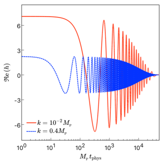
Figure 1: Real part of the gravitational mode amplitude, solution of the simplified Eq. (22), as a function of time, rescaled in units of the Planck time $M_{\mathrm{{}_{P}}}^{-1}$ for two values of the wavenumber, namely $k=10^{-2}M_{\mathrm{{}_{P}}}$ (full line) and $k=0.4M_{\mathrm{{}_{P}}}$ (dashed line) and a Hubble constant set to $H=10^{-4}M_{\mathrm{{}_{P}}}$. Here and in the following, we set $a_{1}=-1$.

IV Initial conditions

From an observational point of view, the last missing piece of the primordial puzzle, also an important characteristics of inflationary predictions, is the tensor spectrum, i.e. the scale distribution of gravitational waves produced during the quasi de Sitter phase. As in the more traditional models, in the context of anomaly-induced quantum gravity, both the scalar and tensor perturbations are generated as quantum vacuum fluctuations subsequently freezing out at Hubble crossing. In what follows, we accordingly set the initial conditions of the tensor mode by assuming it begins in the Bunch-Davies vacuum state; more details about these initial conditions can be found in Grishchuk (1993)) and in Fabris et al. (2012) for the case with anomaly-induced corrections.

The procedure we assume consists in first quantizing the tensor perturbations in the usual way, by merely considering the Einstein-Hilbert action expanded to second order. The canonical creation and annihilation operator expansion then allows to set the vacuum initial condition for the field, which we then generalize to the higher derivative and the anomaly-induced terms.

IV.1 The usual Einstein-Hilbert case

Substituting Eq. (18) into the Einstein-Hilbert action (2), one finds

$$S_{h}=\frac{1}{2}M_{\mathrm{{}_{P}}}^{2}\int\mathrm{d}\eta\,\mathrm{d}^{3}x\,a^{2}(\eta)\left[\left(h^{\prime}_{ij}\right)^{2}-\left(\nabla_{k}h_{ij}\right)^{2}\right],$$ (23)

where a prime denotes a derivative with respect to the conformal time $\eta$. A canonical field formulation is obtained through the following time normalization

$$h_{ij}(\bm{x},\eta)=\frac{\mu_{ij}(\bm{x},\eta)}{a(\eta)M_{\mathrm{{}_{P}}}},$$ (24)

thereby defining $\mu_{ij}$. This transforms Eq. (23), up to an irrelevant time derivative, into

$$S_{\mu}=\frac{1}{2}\int\mathrm{d}\eta\,\mathrm{d}^{3}x\,a^{2}(\eta)\Big{[}\left(\mu^{\prime}_{ij}\right)^{2}-\left(\nabla_{k}\mu_{ij}\right)^{2}+\frac{a^{\prime\prime}}{a}\mu^{2}_{ij}\Big{]},$$ (25)

which corresponds to the action for a scalar field with time-dependent mass. We further decompose $\mu_{ij}$ into two independent modes in Fourier space as

$$\mu_{ij}(\bm{x},\eta)=\int\frac{\mathrm{d}^{3}\bm{k}}{(2\pi)^{3}2k}\mathrm{e}^{i\bm{k}\cdot\bm{x}}\sum_{\lambda=+,\times}\left[\hat{a}^{\lambda}_{\bm{k}}\mu^{\lambda}_{k}(\eta)e^{\lambda}_{ij}(\bm{k})+\hat{a}^{\lambda{\dagger}}_{-\bm{k}}\mu^{\lambda*}_{k}(\eta)e^{\lambda*}_{ij}(-\bm{k})\right],$$ (26)

where we have introduced the polarization tensors $e^{\lambda}_{ij}(\bm{k})$, satisfying the symmetric [$e^{\lambda}_{ij}(\bm{k})=e^{\lambda}_{ji}(\bm{k})$], transverse [$k_{i}e^{\lambda}_{ij}(\bm{k})=0$], traceless [$e^{\lambda}_{ii}(\bm{k})=0$] and orthogonality [$e^{\lambda}_{ij}(\bm{k})e^{\lambda^{\prime}}_{ij}(\bm{k})=\delta^{\lambda\lambda^{\prime}}$] conditions (see Peter (2013) for details on the structure of these tensors).

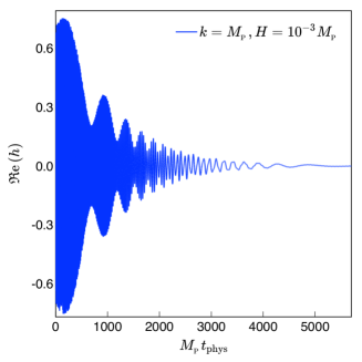
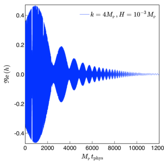
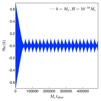
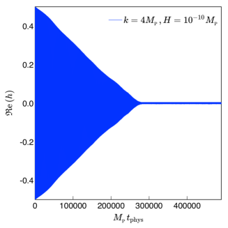
Figure 2: Real part of the gravitational mode solution of the full equation (21) for two distinct de Sitter cases, high (top panel) and low (bottom panel) Hubble rates $H=10^{-3}$ and $H=10^{-10}$ (in Planck units) respectively. Each case shows two Planckian modes, namely $k=1$ (left panel) and $k=4$ (right panel). All plots are for $a_{1}=-1$. The top panels shows that even though the initially increasing mode oscillate tremendously, the damping due to the very rapid background together with the redshifting of the mode wavelength itself manage to suppress the mode amplitude. No runaway solution is found in such a case. The bottom panels on the other hand show that the mode rapidly decreases and is subsequently halted to a constant amplitude due to the fact that the Hubble rate is not large enough to fully compensate for the runaway.

Since Eq. (23) is linear, the expansion (26) plugged back into (25) yields independent contributions from both $+$ and $\times$ modes for each value of the wavenumber $k$. Quantizing can be done on each polarization mode separately as if those were independent scalar fields: the gravitational wave part of the action at second order is nothing but a sum over independent parametric oscillators with time-dependent frequencies, for which the standard rules apply. In particular, one can impose the usual canonical commutation relations on the creation and annihilation operators $\hat{a}^{\lambda}_{\bm{k}}$, $\hat{a}^{\lambda{\dagger}}_{\bm{k}}$. They read

$$\left[\hat{a}^{\lambda}_{\bm{k}},\hat{a}^{\lambda^{\prime}{\dagger}}_{\bm{k}^{\prime}}\right] = (2\pi)^{3}\delta^{\lambda\lambda^{\prime}}\delta(\bm{k}-\bm{k}^{\prime}),$$ (27)

$$\left[\hat{a}^{\lambda}_{\bm{k}},\hat{a}^{\lambda^{\prime}}_{\bm{k}^{\prime}}\right] = 0,$$ (28)

$$\left[\hat{a}^{\lambda{\dagger}}_{\bm{k}},\hat{a}^{\lambda^{\prime}{\dagger}}_{\bm{k}^{\prime}}\right] = 0.$$ (29)

The normalization condition of the mode function $\mu_{k}(\eta)$ is given by that of the Wronskian

$$\mu^{\lambda*}_{k}\partial_{\eta}\mu^{\lambda}_{k}-\mu^{\lambda}_{k}\partial_{\eta}\mu^{\lambda*}_{k}=i,$$ (30)

and from the action (25), we find that the equation of motion for a given mode function, irrespective of the polarization (which is then dropped out of the equation), is given by

$$\mu^{\prime\prime}_{k}+\left(k^{2}-\frac{a^{\prime\prime}}{a}\right)\mu_{k}=0.$$ (31)

As argued above, this is indeed the (or more accurately two copies of the) equation for a parametric oscillator with time-dependent frequency Mukhanov et al. (1992); Peter (2013); Peter and Uzan (2013).

We are now in a position to impose the Bunch-Davies initial conditions for the modes discussed above. For the sub-Hubble modes ($k\gg aH$), one gets the oscillatory behavior typical of the Minkowski vacuum,

$$k\gg aH\ \Longrightarrow\ \mu^{\prime\prime}_{k}+k^{2}\mu_{k}=0\,\Longrightarrow\,\mu_{k}=\frac{\mathrm{e}^{-ik\eta}}{\sqrt{2k}},$$ (32)

while on the other hand, on super-Hubble scales, the modes scales with the scale factor, namely

$$k\ll aH\ \Longrightarrow\ \mu^{\prime\prime}_{k}-\frac{a^{\prime\prime}}{a}\mu_{k}=0\,\Longrightarrow\,\mu_{k}\propto a.$$ (33)

From the mode equation (31), the solution changes from oscillatory to growing at Hubble crossing $k\sim aH$.

IV.2 Seeding the perturbations in the general case

We are now in a position to solve either (21) for the general case or (22), restricting attention as a first approximation to this simpler case. Although the variable $\mu_{k}(t)$ is extraordinary useful to build the actual observational tensor spectrum, we shall only make use of it to provide relevant initial conditions when the extra terms leading to the fourth derivative equation of motion are small.

Let us first expand the actual quantity of interest here, namely the matrix $h(\bm{x},t)$, which we expand in Fourier modes just like its standard counterpart $\mu_{k}(t)$. Assuming fluctuations of the zero point energy of the latter, we find that we can consider an independent mode by writing

$$h(\bm{x},\eta)=h(\eta)\mathrm{e}^{\pm i\bm{k}\cdot\bm{x}}\ \ \ \hbox{and}\ \ \ h(\eta)=\frac{\mathrm{e}^{\pm ik\eta}}{aM_{\mathrm{{}_{P}}}\sqrt{2k}}.$$ (34)

We wrote the last expressions in terms of the conformal time, since it is this time that renders the FLRW metric conformal to the Minkowski metric in flat space; $k$ is the comoving wavenumber vector. After fixing the initial value of the mode $\mu$ and hence $h$, it is a simple matter to derive how the initial amplitude depends on $k$. In our case, in the limit $k\gg aH$, this simplifies to

$$h_{\mathrm{ini}}\varpropto\frac{1}{\sqrt{2k}},\ \ \dot{h}_{\mathrm{ini}}\varpropto\sqrt{\frac{k}{2}},\ \ \ddot{h}_{\mathrm{ini}}\varpropto\frac{k^{3/2}}{\sqrt{2}},\ \ h^{\left(\textsc{\tiny III}\right)}_{\mathrm{ini}}\varpropto\frac{k^{5/2}}{\sqrt{2}}.$$ (35)

Although the initial conditions are set in terms of the conformal time $\eta$, we translate those in terms of the cosmic time $t$ since it is the latter rather than the former which is used in Eqs. (21) and (22). Up to some irrelevant constants of order unity (normalizing the scale factor to one at the initial time) and the Planck mass $M_{\mathrm{{}_{P}}}$, Eq. (35) provides the relevant initial conditions for solving the cases of interest.

V Evolution

We will now rewrite the terms in (22) or (21) using the standard Fourier transform in the space variable, namely we assume the replacement $\bm{\nabla}\to i\bm{k}$ (i.e. $\nabla^{2}\to-k^{2}$). The gravitational waves we are interested in appear during the inflation phase because of the quantum gravitational fluctuations, i.e., the generation of initial seeds of primordial gravity waves by inflation is a quantum process, while their further dynamics can be explored as a classical phenomenon, solving the dynamical equations with quantum initial conditions. We now want to investigate how the perturbation amplitudes in the primordial universe depends of the initial frequency and the background metric dynamics.

For the numerical results presented below, and because the perturbation equations are linear, we have set $M_{\mathrm{{}_{P}}}\to 1$, so that both the amplitude $h$ and the wavenumber $k$ are pure numbers, assumed in units of $M_{\mathrm{{}_{P}}}$. The strategy we adopted consists in the following: first, we consider the simplified version of the mode equation (22) in a de Sitter case, assuming the Hubble rate to be given independently. This is possible since we are interested in the tensor modes, and those do not affect the background evolution at this order. We then move on to the full equation (21) using the MSSM underlying parameters. We also chose to fix the unknown parameter $a_{1}$ to $a^{\mathrm{num}}_{1}=-1$ as it should be negative to avoid tachyonic ghosts; it is subsequently “normalized” for representational convenience.

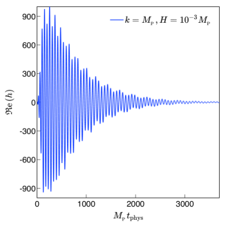
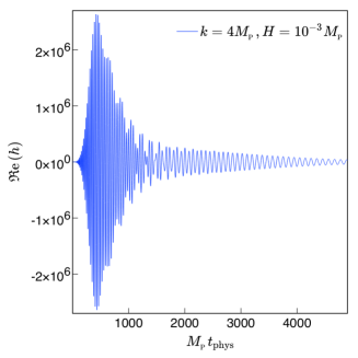
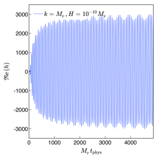
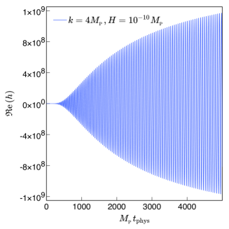
Figure 3: Same as Fig.2 with a radiation dominated background with scale factor behavior $a\varpropto t^{1/2}$. Again, the top panels are for a large initial Hubble scale (now time-varying) $H=10^{-3}$ and the bottom panels for low initial Hubble rate $H=10^{-10}$ (still in Planck units) and the two relevant Planckian modes $k=1$ and $k=4$ are displayed on the left and right panels respectively. It is clear from the figure that the case modes, although initially setting themselves on the runaway ghost solutions, are eventually damped thanks to the large initial value of the Hubble scale, which manages to take up the mode evolution. The growth is however uncontrolled when the initial expansion rate is too low, so the background can keep up with the runaway.

V.1 Higher derivative correction

When one considers only general relativity, i.e. using only $S_{{}_{\mathrm{EH}}}$ of Eq. (2), the initial frequency $k$ hardly changes anything at all in the evolution of the mode except though its normalization. The theory being stable, we find, as expected, so ghost solution whatever the value of either the wavelength $k$ or the Hubble parameter $H$, even for a value as low as the present-day estimate $H=10^{-61}$ and $k$ of order unity.

The vacuum action $S_{\mathrm{vac}}$ of Eq. (4) yields, in practice, a fourth-order differential equation subject to plausible instabilities. Provided $k\ll 1$, one expects to describe the full situation by merely considering this simplified version.

Fig. 1 exemplifies a situation where the Hubble rate is in a reasonable range in which one expects the corrections to have non negligible effects while at the same time not demanding a full quantum gravity theory. In practice, we set $H=10^{-4}$. Such a high value permits to control the unwanted runaway solution: even for rather high wavenumbers, the relevant term in Eq. (22) is proportional to $\nabla^{2}h/a^{2}\to k^{2}h/a^{2}$, and with $a\sim\mathrm{e}^{Ht}$, this contribution goes exponentially fast to negligible values provided the background Hubble rate is sufficiently large.

On the other hand, starting with a trans-Planckian wavelength $k>1$ immediately leads to the ghost taking over the background, and the runaway solution is not possible to stop, at least for reasonable values of the Hubble rate. In order to increase this Hubble rate and figure out the consequence of such an increase, one needs to use the full equation (21) including the anomaly-induced quantum corrections, to which we now turn.

V.2 Anomaly-induced contribution

The same $(k/a)^{2}$ term in Eq. (22) is present in the full version (21), which also contains an additional $(k/a)^{4}$. By the same reasoning, if the expansion is fast enough, these terms rapidly become negligible and one should expect the trans-Planckian runaway to become a non-issue, given a strong enough, sufficiently fast-evolving, background. The case $k<1$ can be studied through the simplified version of (22), which has shown the ghost instability to be essentially irrelevant. It remains to be seen what happens in the more complicated situation where the mode is trans-Planckian, and for this we now discuss the relevant solutions of Eq. (21).

In a first analysis, we studied the de Sitter case under two separate assumptions, namely that the mode is exactly Planckian, i.e., $k=1$, and we then considered the extreme situation with $k>1$, and we set it arbitrarily to $k=4$. For both these modes, we considered either a slow expansion with $H=10^{-10}$, and a fast one with $H=10^{-3}$. Fig. 2 presents these solutions which, we must add, are representative of the general solution and are merely meant to exemplify the underlying results.

We note that for a de Sitter background with $a\varpropto\mathrm{e}^{Ht}$ and $H$ constant, a high value of $H$ induces the following behavior for the mode functions: first, it seems to increase in amplitude, seemingly initiating the ghost instability. Then, the background expanding very rapidly, the $(k/a)^{2}$ and $(k/a)^{4}$ terms are damped to become vanishingly small, and quickly negligible compared to the other terms of Eq. (21). At this point, the mode wavelength has been redshifted sufficiently that it is no longer trans-Planckian and the usual evolution of the previous section takes over. The ghost instability is therefore tamed in this context.

The situation is different when the Hubble rate is much smaller, as exemplified with the case $H=10^{-10}$ and the same mode numbers. In this case, the redshifting is not efficient enough, and although the anomaly-induced terms tend to decrease the amplitude, the effect eventually saturates and the amplitude ends up being constant.

In both cases, one sees the amplitude is slightly smaller for larger initial values of $k$, but this is merely due to the vacuum normalization translated into (35).

Finally, the situation is even more interesting in the case of a radiation dominated universe for which we fix the initial value of the Hubble rate. Again, we find, as shown in Fig. 3, that an initially large expansion rate eventually catches up with the ghost runaway and drives it back to small values. It is unclear however that this could not trigger higher order perturbations and possibly backreaction; this point deserves further examination.

Lastly, a radiation dominated universe with low expansion rate and trans-Planckian modes is definitely problematic as in all cases studied, exemplified in the bottom panels of Fig. 3, as the runaway solution seems to increase unboundedly, with the higher wavenumber implying a larger divergence. At this stage, there does not seem to exist any foreseeable mechanism susceptible to tame this instability.

VI Conclusions

We have studied the anomaly-induced would-be ghost instability in the framework of a FLRW cosmological background with tensor perturbations. As found in a previous works Fabris et al. (2012); Salles and Shapiro (2014), we confirm that sub-Planckian modes on a slowly varying background do not exhibit runaway solutions. Moreover, we find that sub-Planckian on a rapidly varying background also do not exhibit this instability.

The crucial new point concerns the very rapidly expanding background case. In that situation, we found that even trans-Planckian modes can be quickly redshifted and soon become effectively sub-Planckian, so that the background acts as a runaway controller. We have thus obtained a way to tame this otherwise hardly ever mentioned instability, at least in a cosmological context. Given the above argument, we are able to conjecture that the ghost instability may actually be a non-issue in the cosmological setting: if trans-Planckian modes can only be produced in a very rapidly varying background, indeed one for which the anomaly-induced corrections are not negligible, then they will be naturally tamed as in our cosmological examples.

It is easy to indicate the main remaining problems on the way to better description of the role of ghosts in quantum gravity. First of all, it would be very important to study possible realizations of the hypothetic mechanism producing an upper bound on the graviton density Dvali et al. (2011) or alike, both in general and at least on the cosmological background. Second, it would be great to explore the possibility to suppress the growth of tensor modes on other metric backgrounds, capable to develop singularities or at least Planck-order densities of the gravitational field. The existing works on this subject Whitt (1985); Myung (2013); Mauro et al. (2015) are not conclusive and also so not take into account the non-localities. Looking from the general viewpoint, the same mechanism preventing a high density of gravitons Dvali and Gomez (2013) should work in this case. It might happen that the problem can be solved by better understanding non-localities, as it was originally suggested in Tseytlin (1995).

As a final point, we should like to mention that the instabilities that may be generated by the ghosts discussed in this paper potentially arise only at the end of inflation. At this epoch, the non-linear effects are very likely to end up dominating the overall evolution, and thus are expected to modify the physical situation drastically. Therefore, linear perturbation stability cannot, in such a framework, be imposed as an important condition for a consistent theory of gravity.