Moment Approximations and Model Cascades
for Shallow Flow

Abstract

Shallow flow models are used for a large number of applications including weather forecasting, open channel hydraulics and simulation-based natural hazard assessment. In these applications the shallowness of the process motivates depth-averaging. While the shallow flow formulation is advantageous in terms of computational efficiency, it also comes at the price of losing vertical information such as the flow’s velocity profile. This gives rise to a model error, which limits the shallow flow model’s predictive power and is often not explicitly quantifiable. We propose the use of vertical moments to overcome this problem. The shallow moment approximation preserves information on the vertical flow structure while still making use of the simplifying framework of depth-averaging. In this article, we derive a generic shallow flow moment system of arbitrary order starting from a set of balance laws, which has been reduced by scaling arguments. The derivation is based on a fully vertically resolved reference model with the vertical coordinate mapped onto the unit interval. We specify the shallow flow moment hierarchy for kinematic and Newtonian flow conditions and present 1D numerical results for shallow moment systems up to third order. Finally, we assess their performance with respect to both the standard shallow flow equations as well as with respect to the vertically resolved reference model. Our results show that depending on the parameter regime, e.g. friction and slip, shallow moment approximations significantly reduce the model error in shallow flow regimes and have a lot of potential to increase the predictive power of shallow flow models, while keeping them computationally cost efficient.

1 Introduction

Mathematical shallow flow models are successfully applied in a wide range of scientific fields. Since early in the last century they constitute the basis for numerical weather forecasting, an historic overview is given in [20]. Another traditional application is free-surface hydraulics in rivers and channels [11, 6]. In the last decades, new applications emerged, e.g. simulation-based assessment of hazard due to gravity-driven mass movements such as snow avalanches or landslides [7, 29]. Shallow flow models are also relevant beyond geoscience applications and used to compute granular transport processes in chemical engineering, or in production engineering to model coating processes (paints, printing inks, etc), see [8, 16].

In all of these situations shallowness refers to the fact that the flow’s vertical extent is much smaller than its horizontal extent. This motivates the introduction of a suitably chosen vertical average and eventually leads to a depth-averaged model of reduced complexity. Computational costs of shallow flow models are significantly lower than those of a corresponding vertically resolved free-surface flow, which is difficult to solve mainly due to the free surface. The most famous depth-averaged flow model is certainly the shallow water system. In its one dimensional formulation it is traditionally known as the Saint-Venant equations. The idea itself, however, namely deriving a shallow flow model by means of depth-averaging, is not restricted to a constitutive equation representing water and has been applied to many other fluid and granular flow rheologies [33, 15, 2]. Robust and efficient numerical methods have been developed to solve them [27, 38].

Quite naturally any shallow flow formulation comes at the price of loosing vertical information, such as information on the velocity profile. This is not critical if the velocity profile is constant throughout the flow depth and vertical acceleration can be neglected. In the geophysical flow context such a situation is often referred to as ’plug-flow’. In many realistic situations, however, velocity profiles deviate significantly from a vertically constant value. This can be observed both in large scale field experiments [21] as well as in small scale laboratory experiments [34, 32].

The computational shallow flow community encounters this obvious modeling error by introducing the concept of a shape factor. The shape factor is determined based on an assumed parametrization of the velocity profile. Simple polynomial and exponential parametrizations result in shape factors that are independent of field variables, and enter the system as additional constants [18, 22]. Though this serves as a first order correction, it is also restrictive, as the chosen parametrization, say a linear velocity profile, is assumed to be an appropriate choice throughout the duration of the flow. Data acquired during transient granular chute flow experiments again indicate that this is typically not the case and a strong regime dependency of the velocity profile can be observed [34]. The capability to model a regime dependent velocity (and shear) profile would be highly relevant in the geophysical context since it potentially allows erosion rates to be calculated, as well as the coupling forces, both of which are of special interest from an application perspective.

In our work we address this problem and propose a shallow flow formulation based on vertical moments. Moment methods proved to be a powerful tool and have been successfully applied in various scientific fields, such as in rarefied gas dynamics [14, 39]. In the shallow flow context, moment methods allow information on the vertical flow structure to be preserved, while still being able to use depth-averaging to simplify and reduce the complexity of the system. This idea is not entirely new and we follow the spirit of previously published articles on secondary flow effects in curved open channel flow and meandering rivers [13, 37, 40], sediment transport and mixing processes in rivers [1, 12] as well as vertical stratification in shallow geophysical mixtures [23]. While these works focus on pragmatic model derivations that are strongly motivated by specific applications, the focus of our paper is a fundamental analysis and validation of a generic model cascade shallow flows based on moment equations. We complement derivation and analysis of the shallow moment hierarchy with a tailored vertically resolved reference model that will allow us to assess the moment model’s accuracy. The vertically resolved system uses the nonlinear mapping of the shallow flow system onto its scaled counterpart with a constant depth of unity. Such a transformation has been used, e.g., in [26] to study thin melting films in phase-change processes. Since then similar mappings have been applied to a variety of processes, e.g. contact phase-change and ablation processes [25, 36]. Comparing results of the reference system with the shallow flow moment models allows us for the first time to analyze and discuss the model error introduced during depth-averaging. The generic formulation of the shallow flow moment hierarchy and its comparison to the vertically resolved reference solutions are the major innovations of our work.

In Sec. 2 we give a quick overview of the technical approach of the paper. In Sec. 3, we introduce the coordinate mapping and derive the reference shallow flow system. It consists of a first contribution similar to the shallow flow equation, and a second contribution that accounts for a kinematically consistent vertical coupling. We close this section by particularizing the reference shallow flow system for a Newtonian constitutive relation. A moment expansion based on the reference shallow flow system is the content of Sec. 4. In Sec. 5, we present numerical results both for the vertically resolved reference model, and for the shallow moment systems. A different approach to treat the boundary conditions of the vertical velocity profile is given in Sec. 6. We conclude with a summary and a brief outlook. An appendix contains further details of the derivation and equations.

2 Overview of the Approach

In shallow flow scenarios depth-averaging typically means the loss of information about the vertical velocity profile in $z$-direction. The velocity components $u$ and $v$ are replaced by their integral means $u_{m}$ and $v_{m}$. This paper tries to overcome this by assuming a polynomial expansion of the velocity components in the form

$$u(x,y,z,t) =u_{m}(x,y,t)+\sum_{j=1}^{N}\alpha_{j}(x,y,t)\phi_{j}\left(z\right)$$ (1)

$$v(x,y,z,t) =v_{m}(x,y,t)+\sum_{j=1}^{N}\beta_{j}(x,y,t)\phi_{j}\left(z\right)$$ (2)

with appropriate polynomials $\phi_{j}(z)$, $j=1,...,N$, see also [37]. The complete $z$-profile of $u$ and $v$ will now be modeled by the 2d functions $u_{m}(x,y,t)$ and $v_{m}(x,y,t)$ and the coefficients $\alpha_{j}(x,y,t)$ and $\beta_{j}(x,y,t)$ for $j=1,...,N$. The number $N$ will indicate the quality of the model and we will derive concrete partial differential equations for the coefficients for moderate values of $N$ which may replace standard depth-averaged shallow flow models. Additionally, we give the generic formulation of the entire model cascade.

A crucial aspect is the validation of the models and the study of their physical accuracy. For this purpose we derive a tailored reference system that is able to provide synthesized data to evaluate the accuracy of the models in numerical simulations. The reference system is based on non-averaged Navier-Stokes equations, hence vertically resolving the $z$-profiles of the velocity field. Both the reference system and the reduced model cascade assumes hydrostatic equilibrium, hence a linear pressure profile. In this way the reference system can be used to precisely evaluate the error of vertical averaging alone. A version of the reference system using a mapped $z$-coordinate additionally allows a simplified derivation of the model cascade and efficient reference computations.

3 A Reference System for Vertically Resolved Shallow Flow

We use state variables velocity $\mathbf{u}=(u,v,w)^{T}$, pressure $p$ and deviatoric stress tensor $\sigma$ as functions of space $(x,y,z)$ and time $t$. The density $\rho$ is constant and $\mathbf{g}$ is the vector of gravitational acceleration. We allow for a general situation, in which the $z$-axis of the coordinate system is not necessarily collinear with the vector of gravitational acceleration. This implies $\mathbf{g}=[g_{x},g_{y},g_{z}]^{T}=g[e_{x},e_{y},e_{z}]^{T}$, in which $[e_{x},e_{y},e_{z}]^{T}$ is a unit vector and $g$ the value of gravitational acceleration. The Navier-Stokes equations can be reduced by an asymptotic analysis implied by the shallowness assumption. Appendix A shows the basic arguments and, in particular, discusses the influence of the shear stress components $\sigma_{xz}$ and $\sigma_{yz}$ of the stress tensor components, which will be important in the following. As a result of the asymptotic analysis, we will in this work neglect the in-plane deviatoric stresses $\sigma_{xx}$, $\sigma_{yy}$ and $\sigma_{xy}$. Note that these can still have a significant influence in certain granular flow situations, e.g. when they imply a cut-off frequency in the growth rate of roll waves in granular flow, [9], cross-slope velocity gradients due to wall friction [2], and regularization of segregation induced fingers in granular material [3]. In these cases, the shallow moment cascades would have to be extended appropriately.

For now, however, we are interested in study a conceptual shallow flow moment framework on a fundamental level, which is why the resulting system (150) to (153) will be the starting point for the derivation of our reference system as well as for the moment cascade. In order to increase readability we will use the dimensional, yet reduced, formulation of mass and momentum balances, namely

$$\partial_{x}u+\partial_{y}v+\partial_{z}w =0$$ (3)

$$\partial_{t}u+\partial_{x}(u^{2})+\partial_{y}(uv)+\partial_{z}(uw) =-\frac{1}{\rho}\partial_{x}p+\frac{1}{\rho}\partial_{z}\sigma_{xz}+ge_{x}$$ (4)

$$\partial_{t}v+\partial_{x}(uv)+\partial_{y}(v^{2})+\partial_{z}(vw) =-\frac{1}{\rho}\partial_{y}p+\frac{1}{\rho}\partial_{z}\sigma_{yz}+ge_{y}$$ (5)

The dimensional pressure is accordingly given by

$$p(t,x,y,z)=\left(h_{b}(t,x,y)-z\right)\rho ge_{z},$$ (6)

The kinematic boundary conditions (135) and (136) are not affected by back-transformation to dimensional formulation and stay unaltered.

3.1 Mapping

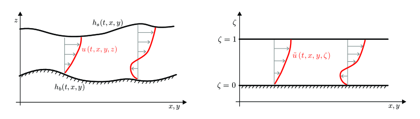
Figure 1: In the physical space (left plot) the flow is constrained in $z$-direction between the basal topography at $z=h_{b}(t,x,y)$ and the free surface at $z=h_{s}(t,x,y)$. The mapping (7) leads to a projected depth coordinate $\zeta$ (right plot) and to a flow that remains in the interval $\zeta\in[0,1]$.

The system (3)-(6) already represents our reference system, however, in order to render it more accessible we formulate the system in terms of the scaled and normalized vertical variable $\zeta$ defined by

$$\zeta =\frac{z-h_{s}(t,x,y)}{h(t,x,y)}$$ (7)

with the height of the flow as $h:=h_{s}-h_{b}$. This kind of mapping immediately implies $z=h(t,x,y)\zeta+h_{b}(t,x,y)$ and effectively transforms the free surface flow onto a domain with a constant height of unity, see Fig. 1. In order to transform the governing equations, we initially consider an arbitrary function depending on space and time $\psi(t,x,y,z)$. Its mapped counterpart $\tilde{\psi}(t,x,y,\zeta)$ is given by

$$\tilde{\psi}\left(t,x,y,\zeta\right) =\psi\left(t,x,y,h(t,x,y)\zeta+h_{b}(t,x,y)\right),$$ (8)

which implies

$$\psi\left(t,x,y,z\right) =\tilde{\psi}\left(t,x,y,h(t,x,y)^{-1}(z-h_{b}(t,x,y))\right).$$ (9)

Later, we want to transform the set of reduced balance laws (3)-(5). This requires differential operators of the mapping $\psi$, which read

$$h\partial_{s}\psi =\partial_{s}\left(h\tilde{\psi}\right)-\partial_{\zeta}\left(\partial_{s}\left(\zeta h+h_{b}\right)\tilde{\psi}\right)\qquad s\in\{t,x,y\}$$ (10)

$$h\partial_{z}\psi =\partial_{\zeta}\tilde{\psi}$$ (11)

3.1.1 Mapping of the Mass Balance

We multiply the mass balance (3) with height $h$

$$h\left(\partial_{x}u+\partial_{y}v+\partial_{z}w\right) =0$$ (12)

and substitute for the partial derivatives according to the transformation rules (10) and (11). This yields the mapped mass balance:

$$\partial_{x}\left(h\tilde{u}\right)+\partial_{y}\left(h\tilde{v}\right)+\partial_{\zeta}\left(\tilde{w}-\partial_{x}\left(\zeta h+h_{b}\right)\tilde{u}-\partial_{y}\left(\zeta h+h_{b}\right)\tilde{v}\right) =0$$ (13)

The mass balance can also be written in integral form to recover an explicit expression for the vertical velocity $\tilde{w}$:

$$\tilde{w} =-\partial_{x}\left(h\int_{0}^{\zeta}\tilde{u}d\hat{\zeta}\right)-\partial_{y}\left(h\int_{0}^{\zeta}\tilde{v}d\hat{\zeta}\right)+\tilde{u}\partial_{x}\left(\zeta h+h_{b}\right)+\tilde{v}\partial_{y}\left(\zeta h+h_{b}\right)$$ (14)

In order to recover the standard depth-averaged continuity equation of the shallow water system, we subtract the vertical velocities at the top and the bottom

$$\tilde{w}(t,x,y,1)-\tilde{w}(t,x,y,0)= -\partial_{x}\left(h\int_{0}^{1}\tilde{u}d\hat{\zeta}\right)-\partial_{y}\left(h\int_{0}^{1}\tilde{u}d\hat{\zeta}\right)$$

$$+\tilde{u}(t,x,y,1)\partial_{x}h_{s}+\tilde{u}(t,x,y,0)\partial_{x}h_{b}$$ (15)

$$+\tilde{v}(t,x,y,1)\partial_{y}h_{s}+\tilde{v}(t,x,y,0)\partial_{y}h_{b}$$

and substitute in the kinematic boundary conditions (135) and (136), which finally results in

$$\partial_{t}h+\partial_{x}\left(hu_{m}\right)+\partial_{y}\left(hv_{m}\right) =0.$$ (16)

Here, we introduced the mean velocity $u_{m}(t,x,y):=\int_{0}^{1}\tilde{u}d\zeta$, and accordingly $v_{m}(t,x,y):=\int_{0}^{1}\tilde{v}d\zeta$, as it is common practice for shallow flow models.

3.1.2 Mapping of the Momentum Balance

Similarly, we multiply the reduced momentum equation (4) with height $h$

$$h\left(\partial_{t}u+\partial_{x}u^{2}+\partial_{y}(uv)+\partial_{z}(uw)\right)+h\frac{1}{\rho}\partial_{x}p =h\frac{1}{\rho}\partial_{z}\sigma_{xz}+hge_{x}$$ (17)

and again substitute according to the transformation rules (10) to (11), which results in the mapped horizontal momentum balance:

$$\partial_{t}\left(h\tilde{u}\right)+\partial_{x}\left(h\tilde{u}^{2}\right)+\partial_{y}\left(h\tilde{u}\tilde{v}\right)$$

$$+\partial_{\zeta}\left(\tilde{u}\left(\tilde{w}-\partial_{t}\left(\zeta h+h_{b}\right)-\tilde{u}\partial_{x}\left(\zeta h+h_{b}\right)-\tilde{v}\partial_{y}\left(\zeta h+h_{b}\right)\right)\right)$$

$$+\frac{1}{\rho}\partial_{x}\left(h\tilde{p}\right)-\frac{1}{\rho}\partial_{\zeta}\left(\tilde{p}\partial_{x}\left(\zeta h+h_{b}\right)\right) =\frac{1}{\rho}\partial_{\zeta}\tilde{\sigma}_{xz}+hge_{x}$$ (18)

Likewise, we can map the hydrostatic pressure relation (6)

$$\tilde{p}\left(x,y,t,\zeta\right) =h\left(x,y,t\right)\left(1-\zeta\right)\rho ge_{z},$$ (19)

which allows us to simplify the pressure dependent terms in (18) according to

$$\frac{1}{\rho}\partial_{x}\left(h\tilde{p}\right)-\frac{1}{\rho}\partial_{\zeta}\left(\partial_{x}\left(\zeta h+h_{b}\right)\tilde{p}\right) =\,\partial_{x}\left(\frac{g}{2}e_{z}h^{2}\right)+hge_{z}\partial_{x}h_{b}.$$ (20)

Interestingly, this expression shows not explicit dependency on the vertical coordinate any longer. Combining (18) and (20) allows to express the mapped horizontal momentum balance concisely as

$$\partial_{t}\left(h\tilde{u}\right)+\partial_{x}\left(h\tilde{u}^{2}+\frac{g}{2}e_{z}h^{2}\right)+\partial_{y}\left(h\tilde{u}\tilde{v}\right)+\partial_{\zeta}\left(h\tilde{u\,}\omega\left[h,\tilde{u},\tilde{v}\right]\right) =\frac{1}{\rho}\partial_{\zeta}\tilde{\sigma}_{xz}+gh\left(e_{x}-e_{z}\,\partial_{x}h_{b}\right).$$ (21)

The vertical coupling operator $\omega$ deserves further attention. By substituting for the vertical velocity (14), we find for the respective term in (18)

$$\tilde{w}-\partial_{t}\left(\zeta h+h_{b}\right)-\tilde{u}\partial_{x}\left(\zeta h+b\right)-\tilde{v}\partial_{y}\left(\zeta h+b\right)$$ (22)

$$=-\partial_{x}\left(h\int_{0}^{\zeta}\tilde{u}d\hat{\zeta}\right)-\partial_{y}\left(h\int_{0}^{\zeta}\tilde{v}d\hat{\zeta}\right)-\zeta\partial_{t}h$$

$$=-\partial_{x}\left(h\int_{0}^{\zeta}\tilde{u}d\hat{\zeta}\right)-\partial_{y}\left(h\int_{0}^{\zeta}\tilde{v}d\hat{\zeta}\right)+\zeta\left(\partial_{x}\left(hu_{m}\right)+\partial_{y}\left(hv_{m}\right)\right)$$

where $u_{m}$ and $v_{m}$ again stand for the mean velocity fields and the integrated mass balance (16) has been used. Introducing $\tilde{u}_{d}(t,x):=\tilde{u}-u_{m}(t,x)$ as well as $\tilde{v}_{d}(t,x):=\tilde{v}-v_{m}(t,x)$ for the deviation from the true velocities $\tilde{u}$ and $\tilde{v}$ we finally obtain

$$h\,\omega\left[h,\tilde{u},\tilde{v}\right] =-\partial_{x}\left(h\int_{0}^{\zeta}\tilde{u}_{d}d\hat{\zeta}\right)-\partial_{y}\left(h\int_{0}^{\zeta}\tilde{v}_{d}d\hat{\zeta}\right)$$ (23)

Note, that we combined terms into $u_{d}$ and $v_{d}$ by writing $\zeta=\int_{0}^{\zeta}d\hat{\zeta}$. For future reference we state an interesting relation for $\omega$ which also clarifies its role as vertical coupling

$$\partial_{x}(h\tilde{u})+\partial_{y}(h\tilde{v})+\partial_{\zeta}(h\omega) =\partial_{x}\left(hu_{m}\right)+\partial_{y}\left(hv_{m}\right)$$ (24)

derived from (23).

Following the same rationale we can derive a mapped y-momentum balance.

3.2 Complete Reference System

All in all, the complete vertically resolved shallow flow system has the form

$$\partial_{t}h+\partial_{x}\left(hu_{m}\right)+\partial_{y}\left(hv_{m}\right) =0,$$ (25)

$$\partial_{t}\left(h\tilde{u}\right)+\partial_{x}\left(h\tilde{u}^{2}+\frac{g}{2}e_{z}h^{2}\right)+\partial_{y}\left(h\tilde{u}\tilde{v}\right)+\partial_{\zeta}\left(h\tilde{u}\omega-\frac{1}{\rho}\tilde{\sigma}_{xz}\right) =gh\left(e_{x}-e_{z}\,\partial_{x}h_{b}\right)$$ (26)

$$\partial_{t}\left(h\tilde{v}\right)+\partial_{x}\left(h\tilde{u}\tilde{v}\right)+\partial_{y}\left(h\tilde{v}^{2}+\frac{g}{2}e_{z}h^{2}\right)+\partial_{\zeta}\left(h\tilde{v}\omega-\frac{1}{\rho}\tilde{\sigma}_{yz}\right) =gh\left(e_{y}-e_{z}\,\partial_{y}h_{b}\right),$$ (27)

with the vertical coupling $\omega$ that can be concisely written as

$$\omega =\frac{1}{h}\overline{\partial_{x}(h\tilde{u})+\partial_{y}(h\tilde{v})}$$ (28)

based on the averaging procedure

$$\overline{\psi} (\zeta)=\int_{0}^{\zeta}\left(\int_{0}^{1}\psi(\check{\zeta})d\check{\zeta}-\psi(\hat{\zeta})\right)d\hat{\zeta}$$ (29)

which follows from (24). The system is evocative of the shallow water equations. This is true for the mass balance, which is formulated in terms of the depth-averaged velocities $u_{m}$ and $v_{m}$. Recall however, that the momentum balance is vertically resolved and the velocity fields $\tilde{u}$ as well as $\tilde{v}$ are functions of the vertical coordinate $\zeta$. Note also that for a constant flow profile in $\zeta$ the vertical coupling coefficient $\omega$ vanishes. In that case, if in addition shear stresses are negligible $\tilde{\sigma}_{xz}=\tilde{\sigma}_{yz}=0$, the system indeed reduces to the shallow water equations.

3.3 Newtonian Closure for the Shallow Flow Reference System

Our numerical examples in Sec. 5 will realize a Newtonian constitutive behavior, which is why we particularize the reference formulation for this situation, see also Sec. A.1 for a discussion of the relevant contributions of the stress tensor. For Newtonian flow the remaining basal shear components of the deviatoric stress tensor are closed according to

$$\sigma_{xz}=\mu\partial_{z}u\qquad\text{and}\qquad \sigma_{yz}=\mu\partial_{z}v$$ (30)

where $\mu$ stand for the material’s dynamic viscosity. Mapping the closure relations (30) according to (11) and writing them in terms of the kinematic viscosity $\nu=\mu/\rho$ yields

$$\frac{1}{\rho}\tilde{\sigma}_{xz}=\frac{\nu}{h}\partial_{\zeta}\tilde{u}\qquad\text{and}\qquad \frac{1}{\rho}\tilde{\sigma}_{yz}=\frac{\nu}{h}\partial_{\zeta}\tilde{v}$$ (31)

which closes the system (25) to (27) for Newtonian flow.

Boundary Conditions: In order to solve it we need to specify dynamic boundary conditions in the form of a velocity boundary condition both at the free-surface $h_{s}$, and at the bottom topography $h_{b}$. At the free-surface we assume stress-free conditions

$$\left.\partial_{z}u\right|_{z=h_{s}}=0\quad\text{and}\left.\partial_{z}v\right|_{z=h_{s}}=0$$ (32)

At the basal surface, we assume slip boundary conditions in the form

$$\left.(u-\frac{\lambda}{\mu}\sigma_{xz})\right|_{z=h_{b}}=0\quad\text{ and }\quad\left.(v-\frac{\lambda}{\mu}\sigma_{yz})\right|_{z=h_{b}}=0$$ (33)

Here, $\lambda$ stands for the slip length and $\mu^{-1}$ has been introduced as a scaling factor for convenience, such that $\lambda$ indeed has the unit of a length scale. A vanishing slip length, $\lambda=0$, results in a no-slip boundary condition, such as commonly applied for Newtonian flow, whereas $\lambda\to\infty$ represents a Neumann boundary condition with prefect slip. Intermediate values of $\lambda$ account for a mixed flow-slip behavior. Substituting for the Newtonian closure (30) transforms the basal boundary condition into

$$\left.(u-\lambda\partial_{z}u)\right|_{z=h_{b}}=0\quad\text{ and }\quad\left.(v-\lambda\partial_{z}v)\right|_{z=h_{b}}=0$$ (34)

and after mapping according to (11) the set of dynamic boundary conditions (32) and (34) read

$$\left.\partial_{\zeta}\tilde{u}\right|_{\zeta=1}=0\qquad\text{and}\qquad \left.\partial_{\zeta}\tilde{v}\right|_{\zeta=1}=0$$ (35)

$$\left.\partial_{\zeta}\tilde{u}\right|_{\zeta=0}=\frac{h}{\lambda}\left.\tilde{u}\right|_{\zeta=0}\qquad\text{and}\qquad \left.\partial_{\zeta}\tilde{v}\right|_{\zeta=0}=\frac{h}{\lambda}\left.\tilde{u}\right|_{\zeta=0}.$$ (36)

4 A Moment Closure for Shallow Flows

We use the mapped reference system for vertically resolved shallow flow to derive a model cascade of dimensionally reduced systems based on moment approximations.

4.1 Averaged Momentum Balance and Polynomial Expansion

The mapped formulation does not only render the numerical discretization of the free-surface flow more accessible, but also allows to directly formulate depth-averaged equations. We will consider the momentum balance (26) with the Newtonian relations (31) but drop the tilde for readability. After integrating $\int_{0}^{1}\cdot d\zeta$ we obtain

$$\partial_{t}\left(hu_{m}\right)+\partial_{x}\left(h\int_{0}^{1}u^{2}d\zeta+\frac{g}{2}e_{z}h^{2}\right)+\partial_{y}\left(h\int_{0}^{1}uvd\zeta\right)-\frac{\nu}{h}[\,\partial_{\zeta}u\,]^{\zeta=1}_{\zeta=0} =hg\left(e_{x}-e_{z}\partial_{x}h_{b}\right)$$ (37)

as evolution equation for the mean velocity $u_{m}$, where we used the fact that the vertical coupling $\omega$ vanishes at the top and the bottom. By substituting for the boundary conditions (35) and (36) we weakly enforce the stick-slip condition

$$-\frac{\nu}{h}[\,\partial_{\zeta}u\,]^{\zeta=1}_{\zeta=0}=\frac{\nu}{\lambda}\left.u\right|_{\zeta=0}$$ (38)

A discussion of the use of weak boundary treatment is presented in Sec. 6 below. Obviously, equation (37) with (38) is not closed as the integrals as well as the evaluation of $u$ at $\zeta=0$ can not be evaluated without further knowledge.

We write both lateral velocity components $u$ and $v$ as a sum of the mean and its deviation, and model the deviation as a finite polynomial expansion, that is,

$$u(x,y,t,\zeta) =u_{m}(x,y,t)+u_{d}(x,y,t,\zeta)=u_{m}(x,y,t)+\sum_{j=1}^{N}\alpha_{j}\left(x,y,t\right)\phi_{j}(\zeta)$$ (39)

$$v(x,y,t,\zeta) =v_{m}(x,y,t)+v_{d}(x,y,t,\zeta)=v_{m}(x,y,t)+\sum_{j=1}^{N}\beta_{j}\left(x,y,t\right)\phi_{j}(\zeta)$$ (40)

where we use a fixed number $N$ of basis functions $\phi_{i}$ and both the mean velocities and the coefficients $\alpha_{j}$ and $\beta_{j}$ are independent of $\zeta$. We employ scaled Legendre polynomials for $\phi_{j}$, orthogonal on the interval $[0,1]$ and normalized by $\phi_{j}(0)=1$. The first three polynomials are given by

$$\phi_{1}(\zeta)=1-2\zeta,\quad\phi_{2}(\zeta)=1-6\zeta+6\zeta^{2} ,\quad\phi_{3}(\zeta)=1-12\zeta+30\zeta^{2}-20\zeta^{3}.$$ (41)

Note, that the mean values $u_{m}$ and $v_{m}$ can be viewed as expansion coefficient for the zeroth basis function which is constant. Increasing the number of coefficients $N$ allows us to describe the vertical profile of the velocity with increasing accuracy.

Using properties of the Legendre polynomials we find

$$\int_{0}^{1}u^{2}d\zeta=u_{m}^{2}+\sum_{j=1}^{N}\tfrac{\alpha_{j}^{2}}{2j+1},\qquad \int_{0}^{1}uvd\zeta=u_{m}v_{m}+\sum_{j=1}^{N}\tfrac{\alpha_{j}\beta_{j}}{2j+1}$$ (42)

and also the evaluation of $u$ at the bottom is easily expressed based on (39) and the normalization condition. We obtain the equation

$$\partial_{t}\left(hu_{m}\right)+\partial_{x}\left(h(u_{m}^{2}+\sum_{j=1}^{N}\tfrac{\alpha_{j}^{2}}{2j+1})+\frac{g}{2}e_{z}h^{2}\right) +\partial_{y}\left(h(u_{m}v_{m}+\sum_{j=1}^{N}\tfrac{\alpha_{j}\beta_{j}}{2j+1})\right)$$

$$=-\frac{\nu}{\lambda}(u_{m}+\sum_{j=1}^{N}\alpha_{j})+hg\left(e_{x}-e_{z}\partial_{x}h_{b}\right)$$ (43)

for $u_{m}$ and averaging the $y$-momentum balance (27) analogously yields$\frac{}{}$

$$\partial_{t}\left(hv_{m}\right)+\partial_{x}\left(h(u_{m}v_{m}+\sum_{j=1}^{N}\tfrac{\alpha_{j}\beta_{j}}{2j+1})\right) +\partial_{y}\left(h(v_{m}^{2}+\sum_{j=1}^{N}\tfrac{\beta_{j}^{2}}{2j+1})+\frac{g}{2}e_{z}h^{2}\right)$$

$$=-\frac{\nu}{\lambda}(v_{m}+\sum_{j=1}^{N}\beta_{j})+hg\left(e_{y}-e_{z}\partial_{y}h_{b}\right)$$ (44)

for the $y$-component $v_{m}$. In case the deviations from the mean can be neglected, all coefficients $\alpha_{i}$ and $\beta_{i}$ vanish and these equations simplify to the well-known shallow flow equation when combined with the equation for $h$ in (25).

4.2 Higher Order Averages

If the deviations can not be neglected we need expressions for the coefficients $\alpha_{i}$ and $\beta_{i}$. By taking moments of the velocity fields with respect to the Legendre polynomials, we obtain

$$\int_{0}^{1}\phi_{i}ud\zeta=\tfrac{\alpha_{i}}{2i+1} \qquad\text{and}\qquad\int_{0}^{1}\phi_{i}vd\zeta=\tfrac{\beta_{i}}{2i+1},$$ (45)

such that we can use the mapped reference equations (26) and (27) to derive moment or evolution equations for $\alpha_{i}$ and $\beta_{i}$. The details are given in Appendix B. The resulting equation for $\alpha_{i}$ is given by

$$\partial_{t}\left(h\alpha_{i}\right)+\partial_{x}\left(h(2u_{m}\alpha_{i}+\sum_{j,k=1}^{N}A_{ijk}\alpha_{j}\alpha_{k})\right)+\partial_{y}\left(h(u_{m}\beta_{i}+v_{m}\alpha_{i}+\sum_{j,k=1}^{N}A_{ijk}\alpha_{j}\beta_{k})\right)$$

$$=u_{m}D_{i}-\sum_{j,k=1}^{N}B_{ijk}D_{j}\alpha_{k}-(2i+1)\frac{\nu}{\lambda}\left(u_{m}+\sum_{j=1}^{N}(1+\frac{\lambda}{h}C_{ij})\alpha_{j}\right)$$ (46)

where the matrices $A_{ijk}$, $B_{ijk}$ and $C_{ij}$ are defined in (155), (158) and (160) of the appendix based on integrals of the Legendre polynomials. The right-hand-side contains non-conservative terms involving the expression

$$D_{i} =\partial_{x}\left(h\alpha_{i}\right)+\partial_{y}\left(h\beta_{i}\right)$$ (47)

that stems from the vertical coupling $\omega$. The analogous equation for $\beta_{i}$ reads

$$\partial_{t}\left(h\beta_{i}\right)+\partial_{x}\left(h(u_{m}\beta_{i}+v_{m}\alpha_{i}+\sum_{j,k=1}^{N}A_{ijk}\alpha_{j}\beta_{k})\right)+\partial_{y}\left(h(2v_{m}\beta_{i}+\sum_{j,k=1}^{N}A_{ijk}\beta_{j}\beta_{k})\right)$$

$$=v_{m}D_{i}-\sum_{j,k=1}^{N}B_{ijk}D_{j}\beta_{k}-(2i+1)\frac{\nu}{\lambda}\left(v_{m}+\sum_{j=1}^{N}(1+\frac{\lambda}{h}C_{ij})\beta_{j}\right)$$ (48)

and exhibits the same structure. Note that $N$ indicates the order of the moment model, while $i$ denotes the actual equation for the specific moment $\alpha_{i}$. Note also, that gravitational forces like the hydrostatic pressure or the bottom topography do not enter these higher order moment equations.

4.3 Examples

In this section, we will look at three specific examples of the model cascade, namely the moment models of zeroth, first and second order. In order to keep things simple, we neglect any influence by the basal topography ($h_{b}=const$) and align the vertical axis of the coordinate system with the negative direction of gravitational acceleration ($e_{x}=e_{y}=0$ and $e_{z}=1$). Additionally, we only present one-dimensional equations.

4.3.1 Zeroth Order System or Shallow Water Equations

The zeroth order shallow moment system then reads

$$\partial_{t}\left(\begin{array}[]{c}h\\ hu_{m}\end{array}\right)+\partial_{x}\left(\begin{array}[]{c}hu_{m}\\ hu_{m}^{2}+g\frac{h^{2}}{2}\end{array}\right)=-\tfrac{\nu}{\lambda}\left(\begin{array}[]{c}0\\ u_{m}\end{array}\right)$$ (55)

For vanishing viscosity ($\nu=0$) it corresponds to homogeneous shallow water flow, which is hyperbolic for positive heights, as the characteristic speeds are given by $a_{1,2}=u_{m}\pm\sqrt{gh}$.

4.3.2 First Order or Linear System

With $s=\alpha_{1}$ indicating the linear contribution to the velocity deviation, the first order shallow moment system reads

$$\partial_{t}\left(\begin{array}[]{c}h\\ hu_{m}\\ hs\end{array}\right)+\partial_{x}\left(\begin{array}[]{c}hu_{m}\\ hu_{m}^{2}+\frac{1}{3}hs^{2}+g\frac{h^{2}}{2}\\ 2hu_{m}s\end{array}\right)=\left(\begin{array}[]{c}0\\ 0\\ u_{m}\partial_{x}(hs)\end{array}\right)-P$$ (65)

with

$$P =\tfrac{\nu}{\lambda}\left(\begin{array}[]{c}0\\ u_{m}+s\\ 3(u_{m}+s+4\frac{\lambda}{h}s)\end{array}\right)$$ (69)

This time the eigenvalues of the flux Jacobian are given by

$$a_{1,2}=u_{m}\pm\sqrt{gh+s^{2}}\qquad\text{and}\qquad a_{3}=u_{m}$$ (70)

again showing that the system is hyperbolic for positive heights. A vanishing first moment $s=0$ leads to the pair of waves that is also present in the shallow flow or zeroth order system.

4.3.3 Second Order or Quadratic System

Considering the parabolic part of the velocity profile indicted by $\kappa=\alpha_{2}$ yields the second order shallow moment system as

$$\partial_{t}\left(\begin{array}[]{c}h\\ hu_{m}\\ hs\\ h\kappa\end{array}\right)+\partial_{x}\left(\begin{array}[]{c}hu_{m}\\ hu_{m}^{2}+\frac{1}{3}hs^{2}+\frac{1}{5}h\kappa^{2}+g\frac{h^{2}}{2}\\ 2hu_{m}s+\frac{4}{5}hs\kappa\\ 2hu_{m}\kappa+\frac{2}{3}hs^{2}+\frac{2}{7}h\kappa^{2}\end{array}\right)=Q\,\partial_{x}\left(\begin{array}[]{c}h\\ hu_{m}\\ hs\\ h\kappa\end{array}\right)-P$$ (83)

with

$$Q=\left(\begin{array}[]{c c c c }0&0&0&0\\ 0&0&0&0\\ 0&0&u_{m}-\tfrac{\kappa}{5}&\frac{s}{5}\\ 0&0&s&u_{m}+\tfrac{\kappa}{7}\end{array}\right)\quad\text{and}\quad P=\tfrac{\nu}{\lambda}\left(\begin{array}[]{c}0\\ u_{m}+s+\kappa\\ 3(u_{m}+s+\kappa+4\frac{\lambda}{h}s)\\ 5(u_{m}+s+\kappa+12\frac{\lambda}{h}\kappa)\end{array}\right).$$ (92)

The structure of the equations is non-unique and there is in principal some flexibility in how the model is split into conservative flux and additional non-conservative contributions of the form $Q\,\partial_{x}V$. We chose the current form inspired by the underlying physical processes, as it follows naturally from the derivation. The flux part in conservation form corresponds to the depth-integrated inertial part of the reference system, whereas the non-conservative contribution corresponds to the depth-integrated vertical coupling factor.

This time, the eigenvalues of the flux Jacobian do not have a simple closed form. They have the form $a=u_{m}+c\sqrt{gh}$ where $c$ is any root of the polynomial

$$c^{4}-\tfrac{10\kappa}{7}c^{3}-\left(1+\tfrac{6\kappa^{2}}{35}+\tfrac{6s^{2}}{5}\right)c^{2} +\left(\tfrac{22\kappa^{3}}{35}-\tfrac{6\kappa s^{2}}{35}+\tfrac{10\kappa}{7}\right)c$$

$$-\tfrac{\kappa^{4}}{35}-\tfrac{6\kappa^{2}s^{2}}{35}-\tfrac{3\kappa^{2}}{7}+\tfrac{s^{4}}{5}+\tfrac{s^{2}}{5}=0$$ (93)

in which $s$ and $\kappa$ have been scaled with $1/\sqrt{gh}$ for better readability.

The hyperbolic properties of the quadratic system are shown in Fig. 2. Its x-axis is given by the scaled second moment $\kappa/\sqrt{gh}$ and the y-axis by the scaled first moment $s/\sqrt{gh}$. Hyperbolicity, hence the existence of a mutual and complete set of real-valued eigenspeeds, is denoted by the green region. Orange stands for a breakdown of hyperbolicity.

We find that the eigenvalues take a particularly simple form for a vanishing second order moment $\kappa=0$. Then, they reduce to

$$a_{1,2}=u_{m}\pm\sqrt{gh+s^{2}}\qquad\text{and}\qquad a_{3,4}=u_{m}\pm\tfrac{s}{\sqrt{3}},$$ (94)

namely a fast wave pair that resembles the fast waves of the linear system (70) and an additional slow wave pair. Also a vanishing first moment $s=0$ guarantees real eigenspeeds, see Fig. 2. Note, that if both first and second moment vanish, hence $s=\kappa=0$, we again recover the shallow flow wave pair.

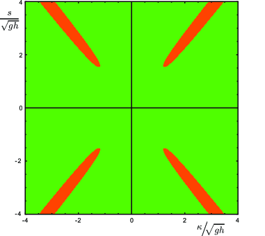
Figure 2: Hyperbolic regions of the quadratic system parametrized in terms of the scaled second moment $\kappa/\sqrt{gh}$ (x-axis) and the scaled first moment $s/\sqrt{gh}$ (y-axis). The green area denotes the existence of a complete set of real valued eigenspeeds, whereas in the orange area imaginary eigenvalues occur.

4.3.4 Third Order or Cubic System

Following the same generic structure as the previous subsections allows to write the cubic system as

$$\partial_{t}V+\partial_{x}F(V)=Q\,\partial_{x}V-P,$$ (95)

with $V=\left(h,hu_{m},hs,h\kappa,hm\right)^{T}$ being the vector of conserved quantities consisting of height $h$, depth-averaged velocity $u_{m}$, and three additional moments $s=\alpha_{1}$,$\kappa=\alpha_{2}$ as well as $m=\alpha_{3}$. Furthermore

$$F(V)=\left(\begin{array}[]{c}hu_{m}\\ hu^{2}_{m}+\tfrac{1}{3}hs^{2}+\tfrac{1}{5}h\kappa^{2}+\tfrac{1}{7}hm^{2}+\tfrac{g}{2}h^{2}\\ 2hu_{m}s+\tfrac{4}{5}hs\kappa+\tfrac{18}{35}h\kappa m\\ 2hu_{m}k+\tfrac{2}{3}hs^{2}+\tfrac{2}{7}h\kappa^{2}+\tfrac{4}{21}hm^{2}+\tfrac{6}{7}hsm\\ 2hu_{m}m+\tfrac{6}{5}hs\kappa+\tfrac{8}{15}h\kappa m\end{array}\right),$$ (101)

$$P=\tfrac{\nu}{\lambda}\left(\begin{array}[]{c}0\\ u_{m}+s+\kappa+m\\ 3\left(u_{m}+\tfrac{h+4\lambda}{h}s+\kappa+\tfrac{h+4\lambda}{h}m\right)\\ 5\left(u_{m}+s+\tfrac{h+12\lambda}{h}\kappa+m\right)\\ 7\left(u_{m}+\tfrac{h+4\lambda}{h}s+\kappa+\tfrac{h+24\lambda}{h}m\right)\end{array}\right)\text{, }Q=\left(\begin{array}[]{c c c c c}0&0&0&0&0\\ 0&0&0&0&0\\ 0&0&u_{m}-\tfrac{\kappa}{5}&\tfrac{s}{5}-\tfrac{3m}{35}&\tfrac{3\kappa}{35}\\ 0&0&s-\tfrac{3m}{7}&u_{m}+\tfrac{\kappa}{7}&\tfrac{2s}{7}+\tfrac{m}{21}\\ 0&0&\tfrac{6\kappa}{5}&\tfrac{4s}{5}+\tfrac{2m}{15}&u_{m}+\tfrac{\kappa}{5}\end{array}\right)$$ (112)

Note, that the hierarchical structure of the moment model is clearly visible, when comparing $F(V)$, $Q$, and $P$ across the cascade of shallow moment systems.

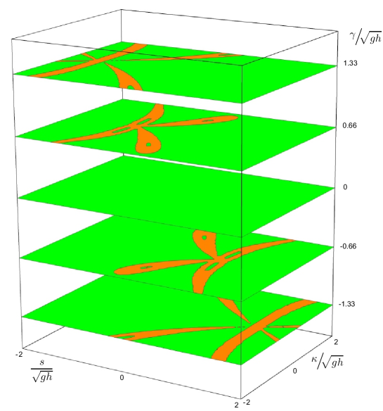
Figure 3: Hyperbolic regions of the cubic system parametrized in terms of the scaled second moment $s/\sqrt{gh}$ (x-axis), the scaled first moment $\kappa/\sqrt{gh}$ (y-axis) and the scaled third moment $m/\sqrt{gh}$ (z-axis). The green area denotes the existence of a complete set of real values eigenspeeds, whereas in the orange area imaginary eigenvalues occur.

Similar to the quadratic system, the eigenvalues of the flux Jacobian are of the form $a=u_{m}+c\sqrt{gh}$ where $c$ this time is the root of an order five polynomial. The complete polynomial is given in the Appendix C. The hyperbolic properties of the cubic system are shown in Fig. 3. Its x-axis is given by the scaled second moment $\kappa/\sqrt{gh}$ and the y-axis by the scaled first moment $s/\sqrt{gh}$ and the z-axis by the scaled thrid moment $m/\sqrt{gh}$. Similar to the previous section, hyperbolicity is denoted by the green region, whereas orange stands for a breakdown of hyperbolicity. Again, we recover a simple form of the eigenvalues for vanishing higher order moments. For $\kappa=m=0$, we get

$$a_{1}=u_{m},\qquad\qquad a_{2,3}=u_{m}\pm\sqrt{gh+s^{2}}\qquad\text{and}\qquad a_{4,5}=u_{m}\pm\sqrt{\frac{3}{7}}s,$$ (113)

with a fast wave pair similar to the linear system (70) that degenerates to the shallow flow wave pair in the case of a vanishing first moment.

4.3.5 Discussion of Hyperbolicity

Hyperbolicity generally implies well-posedness and stability for quasi-linear, first order partial differential equations. On the other hand, the breakdown of hyperbolicity, hence the presence of complex eigenvalues of the transport matrix in certain regions of the state space, can lead to uncontrolled growth of linear instabilities and unwanted grid dependencies. Loss of hyperbolicity is a well known challenge, e.g., for moment models derived from the Boltzmann equation [39] or for generalized, multi-component shallow flow models [30]. In the context of the shallow moment system we deal with in this article, the loss of hyperbolicity may be associated with a degeneracy of the associated vertical velocity profiles or inappropriate projection of these profiles. Note, however, that all numerical test cases presented in Section 5 below have been checked to lay well within the hyperbolic regions of their respective shallow moment system. Throughout the complete duration of the computation, only small values of the higher order moments have been observed.

When applying the shallow moment system to realistic test cases in the future, we will have to put special emphasize on guaranteeing hyperbolicity, hence stability of the system. In particular, this is true for two-dimensional computations, in which oblique wave vectors might lead to additional instabilities.

The breakdown of hyperbolicity can be dealt with in various ways. Different projection-techniques, e.g. based on quadrature [10], may be the most promising option for a stabilizing hyperbolicity fix to the the shallow moment system. An alternative approach proposed in the context of kinetic gas theory relies on a non-linear maximum entropy approach [28].

5 Numerical Simulations

For the simulations presented in this section we consider $h_{b}=const$ and $e_{x}=e_{y}=0$, $e_{z}=1$ as before, and also restrict ourselves to one-dimensional processes. The implementation of these simulations is publicly available on GitHub [24].

5.1 Discretization and Setup

The following numerical simulations will be based on equations in dimensionless form using the scaling of Appendix A.1 with Froude number $F=1$, such that the velocity scale $U$ is given by $\sqrt{gH}$. The scaling replaces the viscosity $\nu$ by a friction coefficient $R=\frac{\nu}{\varepsilon UH}$ representing an inverse Reynolds number scaled by $\varepsilon$, and the slip-length $\lambda$ by the dimensionless constant $\chi=\frac{\lambda}{H}$ . The simulation scenarios both for the reference system of vertically resolved shallow flow equations and the moment approximations are all described by a single setup with details given in Table 1.

Table 1: General setup of the simulation cases for both the vertically resolved equations and its moment approximations in Sec. 5.

$x\in[-1,1],\quad t\in[0,t_{\text{end}}]$	periodic domain, $t_{\text{end}}=2.0$
$h(x,0)=1+\exp\left(3\cos(\pi(x+x_{0}))-4\right)$	initial shift $x_{0}=0.5$
$u(x,0,\zeta)=\begin{cases}0.25&\text{constant case }\\ 0.5\zeta&\text{linear case}\\ 1.5\zeta(1-\zeta)&\text{quadratic case}\end{cases}$	in all cases $u_{m}=0.25$
$R\in\{0,\,0.01,\,0.1\}$ (friction coefficient)	kinematic case uses $R=0$
$\chi\in\{0.01,\,0.1,\,\infty\}$ (slip length)	irrelevant in kinematic case
$n_{x}=160$ (resolution), $\Delta t=0.005$	$n_{\zeta}=80$, for reference system

We consider a periodic domain in which the height is intialized with a nonlinear function describing a bump that rises above the level of $h=1$ to the value of $h\approx 1.36$ in a smooth and periodic way. The velocity $u$ in $x$-direction is constant along $x$ but non-vanishing and we investigate three different depth profiles: constant, linear and quadratic. The linear case corresponds to a shear flow with zero velocity at $\zeta=0$, at least initially. The quadratic case describes a Poiseuille-flow type profile with vanishing velocities both at $\zeta=0$ and $\zeta=1$, again at least initially. All profiles have a mean velocity of $u_{m}=0.25$, such that the collapse of the height bump is super-imposed by a flow to the right. The initial conditions are shifted to the left in order that the barycenter of the result is centered around $x=0$ at time $t_{\text{end}}=2.0$. The values for the friction parameter $R$ and slip length $\chi$ will be varied in the simulation examples. We distinguish between a fully kinematic simulation in which $R=0$ and viscous simulations with $R\neq 0$.

The numerical implementation is straight forward. The moment equations are all discretized based on the explicit high-resolution, third-order finite-volume scheme of [5, 35] with explicit time stepping using a third order stability-preserving Runge-Kutta method. The non-conservative terms are evaluated on cell-centered central differences together with the friction terms in an explicit and non-split manner. The implementation has been validated on simplified scenarios and shows robust empirical convergence upon grid refinement.

The numerical method for the reference system of vertically resolved shallow flow equations is based on the height balance (25) and the momentum balance (26) restricted to one space dimension. Omitting the tilde for scaled variables the system reads

$$\partial_{t}h+\partial_{x}\left(hu\right)+\partial_{\zeta}\left(h\omega\right) =0,$$ (114)

$$\partial_{t}\left(hu\right)+\partial_{x}\left(hu^{2}+\frac{1}{2}h^{2}\right)+\partial_{\zeta}\left(hu\omega\right) =\frac{R}{h}\partial_{\zeta\zeta}u$$ (115)

where we used (24) to replace $u_{m}$ and introduce $\omega$ in the height balance. Per time step this system is split into a hyperbolic left hand side solved explicitly and a diffusive right hand side solved implicitly. For a given vertical coupling $\omega(x,\zeta,t)$ the left part of (114)/(115) is discretized as a hyperbolic system in two dimensions $(x,\zeta)$ using [5, 35] again in a straight forward way. In each time step the identity $\partial_{x}\left(hu\right)+\partial_{\zeta}\left(h\omega\right)=\partial_{\zeta}\left(hu_{m}\right)$ obtained from (24) is discretized and integrated in $\zeta$ by trapezoidal rule on the numerical grid to obtain a new value for the vertical coupling $\omega(x,\zeta,t)$. With this approach also no variations in the $\zeta$-direction will be introduced in the height field $h$. The diffusive term on the right hand side of (115) is discretized implicitly by finite differences. It uses the same cell-centered grid as the finite-volume method and incorporates the boundary conditions

$$\left.\partial_{\zeta}u\right|_{\zeta=0}=\frac{h}{\chi}\left.u\right|_{\zeta=0}\qquad\text{and}\qquad \left.\partial_{\zeta}u\right|_{\zeta=1}=0$$ (116)

with derivatives discretized using one-sided finite differences. As implicit time integrator a single-diagonally implicit Runge-Kutta method of third order is employed, see [17].

All simulations results have been obtained with a $x$-space resolution of $160$ and constant time step $\Delta t=0.005$. For the moment models this implied a CFL number between $0.5$ and $0.6$.

5.2 Reference Solutions

While the actual goal of this section is the study of the moment approximations we will first present results of the system of vertically resolved shallow flow whose solutions will serve as reference for the moment equations.

5.2.1 Kinematic Case

The kinematic equations result form (114)/(115) by setting the friction parameter $R=0$. Boundary conditions can then be ignored because $\omega=0$, both at the bottom and top of the flow. It is important to note that $\omega=0$ holds for any flow constant in $\zeta$ and the equations reduce to the classical shallow flow equations along any line $\zeta=const$. In particular there is no effect that generates a non-constant flow profile in $\zeta$ from a constant one in the kinematic case. Consequently, starting with initial conditions with zero velocity the results will correspond to classical depth-averaged shallow flow. To generate non-trivial results for the kinematic reference equations we consider initial conditions with non-vanishing velocities profiles but same mean velocity as described in Table 1. Recall that under such conditions all three profiles lead to identical (averaged) initial conditions for the standard shallow flow system, such that the impact of the different profiles cannot be studied.

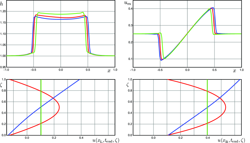
Figure 4: Comparison of height and mean velocity fields (top) together with vertical velocity profiles (bottom) in purely kinematic unsteady solutions of the reference system for shallow flow with three different initial velocity profiles at $t_{\text{end}}=2$, see Table 1: a constant profile (green), a linear profile (blue), and a quadratic profile (red). The velocity profiles shown are taken at position $x_{L}=-0.4$ (left) and $x_{R}=0.4$ (right) of the mean velocity in the upper right plot.

The results of the unsteady computation with the kinematic vertically resolved equations for the three different initial velocity profiles are shown in Fig. 4. The top row displays the height and the mean velocity along the periodic domain in $x$ at $t_{\text{end}}=2.0$. The initial bump has separated into two waves moving left and right that collide with its periodic counterparts. At $t_{end}=2.0$ the two waves have been traveled through each other twice and steepened into two shock waves that move towards the boundaries of the domain. The velocity field shows the typical N-wave shape superimposed on the constant background flow.

The lower row shows the velocity profiles across the normalized mapped domain $\zeta\text{$\in$[0,1]}$ for the three computations at two different positions of the $x$-domain, namely $x_{L}=-0.4$ and $x_{R}=0.4$. The green curves correspond to the constant profile case which is identical to the classical depth-averaged shallow flow equations. It serves also as a reference to identify the influence of the velocity profile. In the kinematic case these differences are small but clearly visible in the results. With both the linear (blue curves) and quadratic (red curves) initial profile the waves travel slightly faster. Consistently, the initially constant profile yields the maximal height at final time, while the bump for both linear and the quadratic profile is less high and wider. In the linear case the two shock waves remain symmetric with respect to the domain’s center as in the classical result, while the quadratic profile leads to a slightly stronger wave on the left.

Over time the velocity profiles in $\zeta$-direction stay very similar to the initial profile. The constant profile remains constant as discussed above. The initially linear profiles exhibits more curvature in the lower plots of Fig. 4, which indicates an active vertical transport. The initially quadratic profile remains vertically symmetric, however, the amplitude of the parabola around its mean varies between the two profile plots in the figure.

5.2.2 Friction Case

To study the effect of friction we consider the same setup as before, see Table 1, but restricted to linear initial profiles. The results are shown in Fig. 5 with the plots arranged in the same way as in Fig. 4 above. The curves only differ in the values of friction and slip coefficients $R$ and $\chi$.

It is instructive to start with the case of a force-free bottom, which is formally obtained by $\chi\to\infty$, such that we have Neumann boundary conditions on either side of $\zeta$, see (116). Given by a non-vanishing parameter $R$, dissipation now leads to an internal equilibration of the initially linear velocity profile that drives the system towards a constant profile case. The red and green curves in Fig. 5 correspond to force-free bottom simulations with friction coefficients $R=0.01$ and $R=0.1$.

Due to friction the profiles become s-shaped during the simulation. The stronger friction case (green) shows an almost constant profile at the end of the simulation (lower row) and the height and mean velocity fields are very similar to the classical shallow flow simulation in Fig. 4. On the other hand, in the lower friction case the linear profile is still recognizable and the result for height and mean velocity shows almost no differences to the friction-less case of Fig. 4.

Introducing the slip-flow boundary conditions (116) with $\chi\neq 0$ significantly influences both the velocity profiles and, consequently, the height and mean velocity fields. The blue and purple curve of Fig. 5 show two results with slip conditions. To maximize the variety of the resulting curves we choose $R=\chi=0.1$ (blue curve) and $R=\chi=0.01$ (purple curve). Especially the result with lower slip coefficient shows a distinct boundary layer in which the velocity profile is pushed towards the value $u=0$. Consequently, the velocity profile exhibits a strongly nonlinear behavior that clearly influences also the curves of height and mean velocity. In tendency, the slip-flow boundary leads to shock waves traveling asymmetrically to the left and right. The force at the bottom also leads to an energy decay and the velocity is relaxing to zero with time.

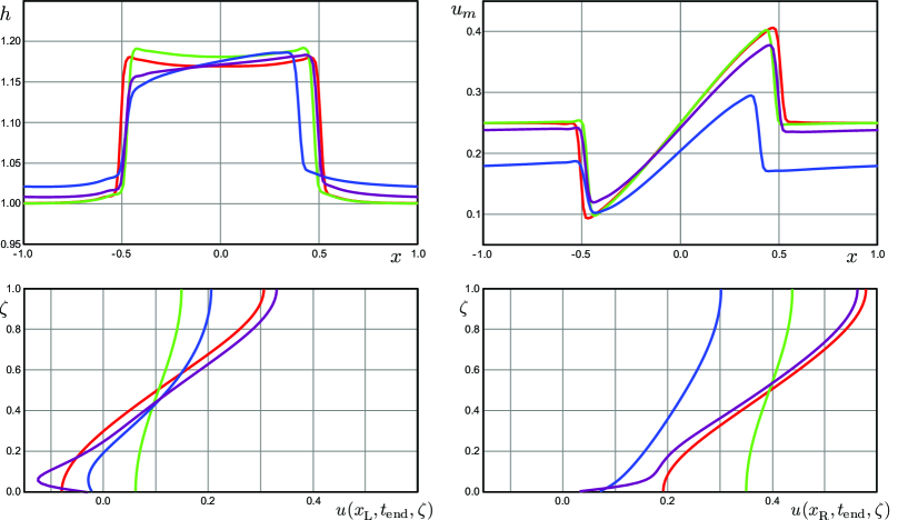
Figure 5: Comparison of height and mean velocity fields (top) together with vertical velocity profiles (bottom) in viscous unsteady solutions of the reference system for shallow flow with linear initial velocity profile at $t_{\text{end}}=2$, see Table 1, and four different setups of friction: force-free bottom, i.e., $\chi=\infty$, with $R=0.01$ (red) and $R=0.1$ (green), finite slip length with the cases $R=\chi=0.1$ (blue) and $R=\chi=0.01$ (purple). The velocity profiles shown are taken at position $x_{L}=-0.4$ (left) and $x_{R}=0.4$ (right) of the mean velocity in the upper right plot.

5.3 Moment Approximations

In order to study the convergence of the model cascade for shallow flow we consider the same general setup as before with an initial bump that separates and interacts with its periodic counterparts, see Table 1. The results will be displayed in Fig. 6 and Fig. 7 that follow the same plot arrangement as above. The test cases are solved by shallow moment systems up to third order: zeroth order system (red curves, Eqn. 55), linear system (green curves, Eqn. 65), quadratic order (blue curves, Eqn. 83), and cubic order system (purple curves). The symbols in the plots denote the reference solution sampled from results of the vertically resolved reference solutions discussed in Sec. 5.2. Higher order moments are reconstructed from the vertically resolved velocity profile.

Note, that the zeroth order system corresponds to the classical shallow flow system. For each test case we can hence assess the moment hierarchy’s performance with respect to both the standard shallow flow model (red) as well as with respect to the vertically resolved reference solution (symbols). As a rough estimate of the computational efficiency of the moment approximations we state the following relative run times for the test cases of Table 1:

Theory	Shallow Flow	Linear System	Quadratic	Cubic	Reference System
Run Time	$1.0$	$1.7$	$2.3$	$3.8$	$\approx 100.0$

Note, that both moment, and reference implementation may allow further performance optimizations.

5.3.1 Kinematic Case

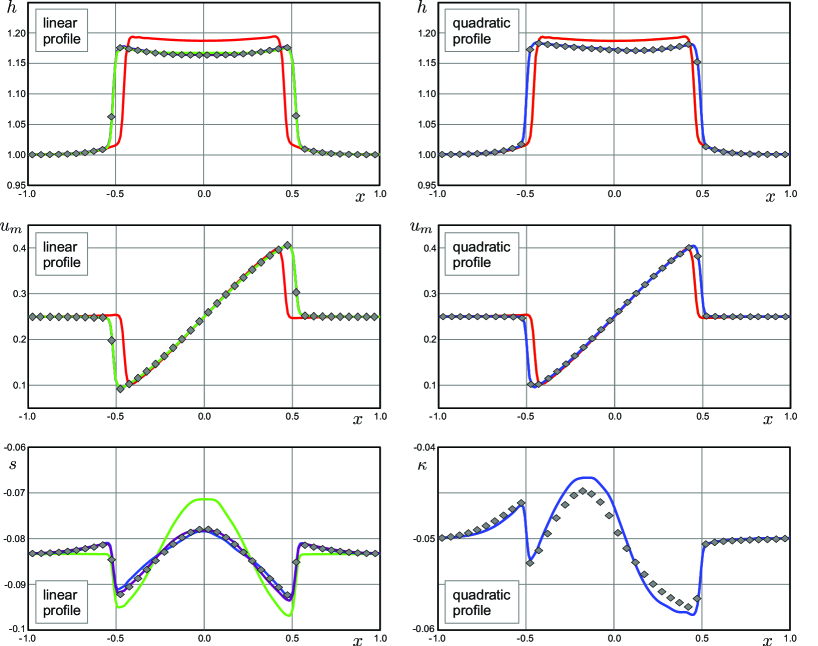
Figure 6: Moment approximations for shallow flow in purely kinematic unsteady solutions with linear (left column) and quadratic (right column) initial velocity profiles at $t_{\text{end}}=2$, see Table 1. The height and mean velocity are shown in the first and second row, and the bottom row displays the fields of first and second moment, respectively. Symbols represent the result of the vertically resolved reference simulation, while the lines represent classical shallow flow equations (red), as well as the linear (green), the quadratic (blue) and the cubic (purple) moment system.

Resembling the structure of the previous discussion in Sec. 5.2, we consider the kinematic case ($R=0$) first. Numerical results are shown in Fig. 6. The left column displays the results for a linear initial velocity profile, whereas the right column shows the results of a parabolic initial velocity profile. Top and second row show height and mean velocity fields. For the linear initial velocity profile (left column) we additionally display the first moment in the bottom row. As discussed earlier, see Sec. 5.2.1, a parabolic initial velocity profile does not generate any linear contribution in the kinematic case such that the first moment remains identically zero. Consequently, it is instructive to analyze the second moment for an initially parabolic velocity profile (bottom right).

While for the linear initial velocity profile the zeroth order moment system (shallow water system) differs clearly visible from the reference solution, we observe that linear and higher order systems are almost perfectly aligned with the reference solution for height and mean velocity. Only the height (upper left) of the linear system (green) deviates slightly around the domain’s center. Numerical results of the first moment (bottom left) allow further insight. Note, that the first moment of the zeroth order system naturally vanishes such that there is no red curve in this plot. The remaining curves nicely show convergence of the moment hierarchy with increasing order. While the linear system still over- and undershoots the reference solution significantly, the quadratic and especially the cubic order system capture the first moment pattern much better.

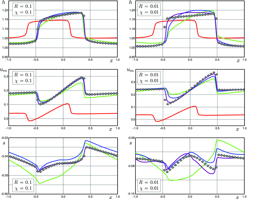
Figure 7: Moment approximations for shallow flow in viscous unsteady solutions with linear initial velocity profiles at $t_{\text{end}}=2$, see Table 1. The left column uses $R=\chi=0.1$, and the right column uses $R=\chi=0.01$. The rows show height, mean velocity and the first moment. Symbols represent the result of the vertically resolved reference simulation, while the lines represent classical shallow flow equations (red), as well as the linear (green), the quadratic (blue) and the cubic (purple) moment system.

For the initially parabolic velocity profile we again observe that height and mean velocity of the zeroth order system differ significantly from the reference solution. Only this time, we cannot see any improvement by using the linear system. In fact both overlap exactly, that is, the green curves lies behind the red. This makes sense as for a zero first moment $s=0$ the linear system (65) reduces to the zeroth order system (55). The quadratic system agrees very nicely with the reference solution, while the cubic result is again identical to the quadratic. This time the second moment (lower right) allows further insight. It naturally vanishes in both zeroth and first order system (absence of red and green curve in the plot). The second moment calculated with the quadratic order system captures the reference solution nicely except for occasional over- and undershooting. The cubic order system yields no further improvement, and simply reproduces the results of the quadratic system such that the purple curve is covered in the plot. In this case further improvement is only expected for the fourth order moment system, which is not considered in our work.

5.3.2 Friction Case

The full benefit of the shallow moment hierarchy becomes evident when including friction. Here, we concentrate on two slip-flow parameter settings corresponding to $R=\chi=0.1$ (left column) and $R=\chi=0.01$ (right column). In both test cases the initial velocity profile is linear. The corresponding vertically resolved reference solution has been discussed in Sec. 5.2.2. The results of the moment models is shown in Fig. 7. In each column the plots are given by height, mean velocity and first moment in the top, middle and bottom rows. We observe that the zeroth order moment system (classical shallow flow theory in red) cannot capture the bump’s shape at final time adequately at all. For neither of the two parameter settings it can reproduce the flow’s height, its mean velocity, or the position of the bump at final time.

The larger slip length case $\chi=0.1$ (left column) already benefits significantly from using the linear system (green). Height and position of the right-going shock wave match the reference solution. The plot of the first moment (bottom left), however, reveals that there is still a significant discrepancy around the left going wave. This error gets smaller when increasing the order of the moment system (blue and purple curves). As expected it is the cubic system that yields the most accurate result, indicating a converging behavior of the moment hierarchy.

As we decrease the slip length $\chi=0.01$ (right column) the linear system (green) can still correctly capture the position of the right-going wave, but it predicts the mean velocity field less accurately, especially maximum and minimum velocities. Considering the first moment (bottom right) the situation gets even worse. Here, the linear system even fails to qualitatively capture the behavior. The linear system results in an N-shaped profile, while the reference solution shows an W-shaped first moment that indicates the presence of strong nonlinearities given by the boundary layer, see Sec. 5.2.2. Again, we observe that the quadratic, and eventually the cubic system increase model accuracy and correctly account for the aforementioned W-shape of the first moment. The absolute model error is however larger with decreasing slip length.

6 Strong Enforcement of Boundary Conditions

The boundary conditions of the velocity profile at the bottom and at the free surface have only been weakly enforced in the moment approximations of Sec. 4 using partial integration of the friction terms. It is also possible to impose the boundary conditions (35)/(36) directly onto the polynomial ansatz (39)/(40). This gives the linear equations

$$\sum_{j=1}^{N}j(j+1)(-1)^{j}\alpha_{j}=0,\qquad \sum_{j=1}^{N}(j(j+1)\lambda+h)\alpha_{j}=-hu_{m}$$ (117)

as constraints to the variables $\{\alpha_{j}\}_{j=1,...N}$. An analogous expression holds for the variables $\{\beta_{j}\}_{j=1,...N}$ involving mean velocity $v_{m}$. Using these equations to express the two largest coefficients $\alpha_{N-1,N}$ and $\beta_{N-1,N}$ as functions of the lower order variables allows to formulate a reduced $N(\star)=N-2$ moment approximation. The projection of the Newtonian friction terms $\partial_{\zeta\zeta}u$ and $\partial_{\zeta\zeta}v$ can then be directly evaluated without partial integration.

This approach also comes with disadvantages. The elimination of variables strongly increases the nonlinearity of the equations making it difficult to to write an explicit cascading form of a generic $N(\star)$-system. Also, an explicit space dependence is introduce into the flux function, since the constraint equations involve the possibly space dependent slip-length $\lambda$ in general. Additionally, the direct projection of the friction will in general not yield symmetric positive definite matrices as in the weak case. However, an increased approximation quality for cases with friction can be expected.

We evaluate conditions (117) for $N=3$ in one space dimension and as before use $s=\alpha_{1}$, $\kappa=\alpha_{2}$, and $m=\alpha_{3}$ for the coefficients. The explicit relations for the higher order moments then read

$$\kappa=-\frac{5s+6u_{m}}{9(1+8\lambda/h)},\qquad m=-\frac{4s(1+3\lambda/h)+3u_{m}}{9(1+8\lambda/h)}$$ (118)

which we will further simplify to the non-slip case by setting $\lambda=0$. Using these no-slip relations in the cubic system (95)/(101) and droping the two highest equations, we arrive at the relatively compact cubic($\star$) no-slip moment system

$$\partial_{t}\left(\begin{array}[]{c}h\\ hu_{m}\\ hs\end{array}\right)+\partial_{x}\left(\begin{array}[]{c}hu_{m}\\ \frac{116}{105}hu_{m}^{2}+\frac{80}{189}hs^{2}+\frac{4}{21}hu_{m}s+g\frac{h^{2}}{2}\\ \frac{4}{35}hu_{m}^{2}-\frac{20}{63}hs^{2}+\frac{12}{7}hu_{m}s\end{array}\right)=\left(\begin{array}[]{c}0\\ 0\\ \frac{8u_{m}}{7}\partial_{x}(hs)-\frac{s}{7}\partial_{x}(hu_{m})\end{array}\right)-P$$ (128)

using only the moment variable $s$ next to height $h$ and mean velocity $u_{m}$. The direct evaluation of the friction terms based on the constrained cubic polynomial yields the expression

$$P =\frac{\nu}{h}\left(\begin{array}[]{c}0\\ 8u_{m}+\frac{20}{3}s\\ 20u_{m}+\frac{80}{3}s\end{array}\right)$$ (132)

for the production.

This cubic($\star$) no-slip system is based on a third degree polynomial for the vertical velocity which will automatically satisfy free-force conditions at the surface and vanishing velocity at the bottom. The remaining flexibility of the profile is encoded into the mean velocity and the linear moment $s$. In Fig. 8 we show the result of the system for the test case of Table 1 with friction coefficient $R=0.01$ and dimensionless slip length $\chi=0.01$. Note that the cubic($\star$) system (128) formally assumes $\chi=0$, but is used here in an approximative way. The figure shows good approximation of the reference data. In particular, the quality of the result is clearly better than the original linear system which uses the same number of equations and better than the original cubic system with weak boundary conditions which uses the same underlying polynomial degree. Note, that using the constraint equations (118) with the precise slip length $\chi=0.01$ would not show any visible improvement in the result. Further approximation quality can be achieved by increasing the underlying polynomial degree together with the contrainst (117), which is left to future work.

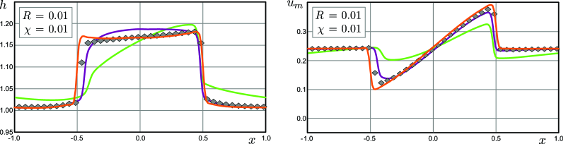
Figure 8: Moment approximations with strongly enforced no-slip boundary conditions in the underlying vertical velocity profile (orange lines). Test case of viscous unsteady solutions with linear initial velocity profiles at $t_{\text{end}}=2$ and friction parameters $R=\chi=0.01$, see Table 1. Symbols represent the result of the vertically resolved reference simulation, while the other lines represent the linear (green) and cubic (purple) moment system with weak boundary conditions (as in Fig. 7)

7 Conclusions

In this article, we investigated mathematical models for shallow flow systems. We conducted a scaling analysis of the fundamental balance laws that reflects the process’s shallow geometry and allows to identify dominant terms. We formulated the resulting mathematical equations as a vertically resolved reference system, which gave us direct access to deriving a vertical model cascade for shallow flows based on moment approximations. The model cascade was exemplified for purely kinematic, nonviscous conditions as well as for Newtonian flow, in which a slip boundary condition at the bottom topography has been weakly enforced. Finally, we presented numerical results in 1D for both the kinematic, and for the Newtonian flow situation. The performance of the shallow flow moment cascade up to third order has been investigated with respect to both the classical shallow flow theory, and with respect to the fully vertically resolved reference model. In a final example, we consider a shallow flow moment variant that strongly enforces the basal and free-surface boundary conditions. We found that many shallow flow regimes cannot be adequately captured with the standard shallow flow theory. This is typically true for a flow situation that is governed by a complex velocity profile, e.g. induced by friction or by forced in-flow. By using shallow flow moment systems, we can significantly improve the validity of the mathematical model. Our test cases consistently showed a converging behavior of the moment hierarchy.

Similar to the classical shallow flow equations, the shallow moment hierarchy makes use of the complexity reducing framework of depth-averaging. Other than the standard shallow flow theory, however, it preserves information on the vertical flow structure similar to a fully vertically resolved mathematical model, yet being computationally less costly. For physical flow regimes, in which the classical shallow flow model results in a large model error and fails, it constitutes a powerful alternative to improve on the predictive power of shallow flow simulations in the future.

Appendix A Dimensional Analysis

We consider incompressible flow in three dimensions, for which mass and momentum can be written as

$$\nabla\cdot\mathbf{u} =0$$ (133)

$$\partial_{t}\mathbf{u}+\nabla\cdot(\mathbf{u}\mathbf{u}) =-\frac{1}{\rho}\nabla p+\frac{1}{\rho}\nabla\cdot\sigma+\mathbf{g}$$ (134)

The state variables velocity $\mathbf{u}=(u,v,w)^{T}$, pressure $p$ and deviatoric stress tensor $\sigma$ are functions of space $(x,y,z)$ and time $t$. The density $\rho$ is constant and $\mathbf{g}$ is the vector of gravitational acceleration. We allow for a general situation, in which the $z$-axis of the coordinate system is not necessarily collinear with the vector of gravitational acceleration. This implies $\mathbf{g}=[g_{x},g_{y},g_{z}]^{T}=g[e_{x},e_{y},e_{z}]^{T}$, in which $[e_{x},e_{y},e_{z}]^{T}$ is a unit vector and $g$ the value of gravitational acceleration. The often used shallow water coordinate system is recovered by choosing $e_{x}=e_{y}=0$ and $\mathbf{g}=g[0,0,-1]^{T}$. The flowing material is bounded by the basal topography $h_{b}(t,x,y)$ and the upper free surface $h_{s}(t,x,y)$. In the absence of mass production at the ground, $h_{b}$ will be a function of $x$ and $y$ alone and has no explicit time dependency. However, we formally allow the basal topography to be time dependent, which allows to write the kinematic boundary conditions for the material boundaries $h_{b}$ and $h_{s}$ in a symmetric way following [31]

$$\partial_{t}h_{s}+\left(u(t,x,y,h_{s}),v(t,x,y,h_{s})\right)^{T}\cdot\nabla h_{s} =w(t,x,y,h_{s})$$ (135)

$$\partial_{t}h_{b}+\left(u(t,x,y,h_{b}),v(t,x,y,h_{b})\right)^{T}\cdot\nabla h_{b} =w(t,x,y,h_{b}).$$ (136)

See also Fig. 1 for a sketch of the situation in one dimension.

A.1 Scaling

We are interested in free-surface shallow flow, which is characterized by a horizontal length scale $L$ that is much larger than the characteristic vertical length scale $H$, hence $H/L=\epsilon<<1$. Consequently, we scale

$$x =L\hat{x},\quad y=L\hat{y},\quad z=H\hat{z}.$$ (137)

We furthermore assume a characteristic horizontal velocity scale given by a generic velocity $U$. According to the shallowness the vertical velocity will be much smaller, which suggests $\epsilon U$ as a characteristic vertical velocity scale

$$u =U\hat{u},\quad v=U\hat{v},\quad w=\epsilon U\hat{w}.$$ (138)

An appropriate time scale is then given by the ratio of spatial and velocity scale

$$t =\frac{L}{U}\hat{t}.$$ (139)

This scaling is motivated by our primary interest in velocity profiles and $U$ can be specified later. An often used specific choice is the free-fall time scale $T=\sqrt{L/g}$ which is based on $U=\sqrt{gL}$.

Finally, we introduce characteristic stresses. Here, we assume that the pressure scales with the hydrostatic pressure based upon the characteristic height $H$ and stresses $\sigma$ with a characteristic stress $S$. Furthermore, we assume that the basal shear stresses $\sigma_{xz}$ and $\sigma_{yz}$ are of larger order in the shallowness parameter $\epsilon$ than lateral shear stresses $\sigma_{xy}$ and normal shear stresses $\sigma_{kk},\,k\in\{x,y,z\}$, that is,

$$p =\rho gH\hat{p},\quad\sigma_{xz/yz}=S\hat{\sigma}_{xz/yz},\quad\sigma_{xx/xy/yy/zz}=\epsilon S\hat{\sigma}_{xx/xy/yy/zz}.$$ (140)

This is an appropriate assumption for many rheologies relevant to our focus area, namely shallow flow in the geophysical context, as these often scale linearly with the strain rate $\dot{\gamma}$. Upon applying the shallow flow scaling (137) and (138), we find for the the strain rate

$$\dot{\gamma}=\frac{U}{H}\left(\begin{matrix}2\epsilon\partial_{\hat{x}}\hat{u}&\epsilon\left(\partial_{\hat{y}}\hat{u}+\partial_{\hat{x}}\hat{v}\right)&\partial_{\hat{z}}\hat{u}+\epsilon^{2}\partial_{\hat{x}}\hat{w}\\ \epsilon\left(\partial_{\hat{x}}\hat{v}+\partial_{\hat{y}}\hat{u}\right)&2\epsilon\partial_{\hat{y}}\hat{v}&\partial_{\hat{z}}\hat{v}+\epsilon^{2}\partial_{\hat{y}}\hat{w}\\ \partial_{\hat{z}}\hat{u}+\epsilon^{2}\partial_{\hat{x}}\hat{w}&\partial_{\hat{z}}\hat{v}+\epsilon^{2}\partial_{\hat{y}}\hat{w}&2\epsilon\partial_{\hat{z}}\hat{w}\end{matrix}\right)$$ (141)

Neglecting all terms that scale with $\epsilon$ leads to the well-known boundary layer approximation:

$$\dot{\gamma}=\frac{U}{H}\left(\begin{matrix}0&0&\partial_{\hat{z}}\hat{u}\\ 0&0&\partial_{\hat{z}}\hat{v}\\ \partial_{\hat{z}}\hat{u}&\partial_{\hat{z}}\hat{v}&0\end{matrix}\right)$$ (142)

For our purposes this is too restrictive, though. Instead, we will keep terms of first order in $\epsilon$ but drop terms of second order in $\epsilon^{2}$, which directly motivates the scaling introduced in (140). The relevance of this assumption is demonstrated by two examples:

• Newtonian flow: In the case of incompressible Newtonian shallow flow, the deviatoric stress is given by

  $$\sigma=2\mu\dot{\gamma}=2\mu\frac{U}{H}\hat{\dot{\gamma}}.$$ (143)

  With a characteristic stress defined as $S=\mu\frac{U}{H}$ we recover the postulated scaling (140).

• Granular flow: Similarly, the plastic deformation of dense granular flow is governed by a constitute relation that scales linearly with the strain-rate tensor. It is given by the so-called $\mu(I)$ rheology [19], which is defined as

  $$\sigma=\mu(I)\frac{p}{|\dot{\gamma}|}\dot{\gamma}$$ (144)

  Here, $\mu(I)$ is a generalized friction coefficient formulated in terms of the inertial number $I$, the ratio of macroscopic deformation time scale and grain inertial time scale. Furthermore, $|\dot{\gamma}|$ stands for the second invariant of the strain rate tensor $\dot{\gamma}$. It has been shown that the $\mu(I)$-rheology is well-posed only for intermediate values of the inertial number [4], while a depth-averaged formulation like [15] have much better properties. Generally, this invariant is likewise affected by the shallow flow scaling (137) and (138), but has leading terms of zero order in $\epsilon$:

  $$|\dot{\gamma}|=\frac{U^{2}}{4H^{2}}\left((\partial_{\hat{z}}\hat{u})^{2}+(\partial_{\hat{z}}\hat{v})^{2}\right)+\mathcal{O}(\epsilon^{2})$$ (145)

  Hence, characteristic stress $S$ defined as $\mu(I)\frac{p}{|\dot{\gamma}|}$ is independent of $\epsilon$ and we again recover the scaling postulated in (140).

A.2 Dimensionless System

All in all, the componentwise mass and momentum equations written in scaled dimensionless coordinates read

$$\partial_{\hat{x}}\hat{u}+\partial_{\hat{y}}\hat{v}+\partial_{\hat{z}}\hat{w} =0$$ (146)

$$F^{2}\epsilon\left(\partial_{\hat{t}}\hat{u}+\partial_{\hat{x}}\hat{u}^{2}+\partial_{\hat{y}}(\hat{u}\hat{v})+\partial_{\hat{z}}(\hat{u}\hat{w})\right) =-\epsilon\partial_{\hat{x}}\hat{p}+\epsilon^{2}G\partial_{\hat{x}}\hat{\sigma}_{xx}+\epsilon G\partial_{\hat{y}}\hat{\sigma}_{xy}+G\partial_{\hat{z}}\hat{\sigma}_{xz}+e_{x}$$ (147)

$$F^{2}\epsilon\left(\partial_{\hat{t}}\hat{v}+\partial_{\hat{x}}(\hat{u}\hat{v})+\partial_{\hat{y}}(\hat{v}^{2})+\partial_{\hat{z}}(\hat{v}\hat{w})\right) =-\epsilon\partial_{\hat{y}}\hat{p}+\epsilon G\partial_{\hat{x}}\hat{\sigma}_{xy}+\epsilon^{2}G\partial_{\hat{y}}\hat{\sigma}_{yy}+G\partial_{\hat{z}}\hat{\sigma}_{yz}+e_{y}$$ (148)

$$F^{2}\epsilon^{2}\left(\partial_{\hat{t}}\hat{w}+\partial_{\hat{x}}(\hat{u}\hat{w})+\partial_{\hat{y}}(\hat{v}\hat{w})+\partial_{\hat{z}}\hat{w}^{2}\right) =-\partial_{\hat{z}}\hat{p}+\epsilon G\partial_{\hat{x}}\hat{\sigma}_{xz}+\epsilon G\partial_{\hat{y}}\hat{\sigma}_{yz}+\epsilon G\partial_{\hat{z}}\hat{\sigma}_{zz}+e_{z}$$ (149)

in which $F=U/\sqrt{gH}$ stands for the Froude number and $G=S/\rho gH$ for the ratio between characteristic stress and characteristic hydrostatic pressure. Note that for a Newtonian constitutive relation ($S=\mu U/H$) and a Froude Number close to one ($U^{2}\approx gH$), the parameter $G$ reduces to the inverse of the well-known Reynolds Number, namely $G=\nu/(HU)$, with $\nu$ standing for the kinematic viscosity $\mu/\rho$.

In regimes in which the stress is dominated by hydrostatic pressure we have $G<1$, and hence contributions of the order $\epsilon^{2}$ and $\epsilon G$ will be insignificant. The system can then be reduced to

$$\partial_{\hat{x}}\hat{u}+\partial_{\hat{y}}\hat{v}+\partial_{\hat{z}}\hat{w} =0$$ (150)

$$F^{2}\epsilon\left(\partial_{\hat{t}}\hat{u}+\partial_{\hat{x}}\hat{u}^{2}+\partial_{\hat{y}}(\hat{u}\hat{v})+\partial_{\hat{z}}(\hat{u}\hat{w})\right) =-\epsilon\partial_{\hat{x}}\hat{p}+G\partial_{\hat{z}}\hat{\sigma}_{xz}+e_{x}$$ (151)

$$F^{2}\epsilon\left(\partial_{\hat{t}}\hat{v}+\partial_{\hat{x}}(\hat{u}\hat{v})+\partial_{\hat{y}}(\hat{v}^{2})+\partial_{\hat{z}}(\hat{v}\hat{w})\right) =-\epsilon\partial_{\hat{y}}\hat{p}+G\partial_{\hat{z}}\hat{\sigma}_{yz}+e_{y}$$ (152)

$$0 =-\partial_{\hat{z}}\hat{p}+e_{z}.$$ (153)

From the reduced vertical momentum balance (153), we can directly solve for the pressure profile

$$\hat{p}(\hat{t},\hat{x},\hat{y},\hat{z})=\left(\hat{h}_{s}(\hat{t},\hat{x},\hat{y})-\hat{z}\right)e_{z}$$ (154)

which satisfies a stress-free boundary condition at the free surface $\hat{p}(\hat{t},\hat{x},\hat{y},\hat{h}_{s}(\hat{t},\hat{x},\hat{y}))=0$. This system forms the starting point of Sec. 3 in the main text.

Appendix B Higher Order Moment Equations

For completeness we present the details of deriving the equation (46) for the higher order expansion coefficients $\alpha_{i}$. Defining

$$A_{ijk}=(2i+1)\int_{0}^{1}\phi_{i}\,\phi_{j}\,\phi_{k}\,d\zeta$$ (155)

we can write

$$\int_{0}^{1}\phi_{i}u^{2}d\zeta =\tfrac{1}{2i+1}(2u_{m}\alpha_{i}+\sum_{j,k=1}^{N}A_{ijk}\alpha_{j}\alpha_{k})$$ (156)

and

$$\int_{0}^{1}\phi_{i}uvd\zeta =\tfrac{1}{2i+1}(u_{m}\beta_{i}+v_{m}\alpha_{i}+\sum_{j,k=1}^{N}A_{ijk}\alpha_{j}\beta_{k})$$ (157)

for the moments of the convective terms in (26). For the vertical coupling term we define

$$B_{ijk}=(2i+1)\int_{0}^{1}\phi_{i}^{\prime}\,\left(\int_{0}^{\zeta}\phi_{j}\,d\hat{\zeta}\right)\,\phi_{k}\,d\zeta$$ (158)

such that we can write

$$\int_{0}^{1}\phi_{i}\,\partial_{\zeta}\left(hu\omega\left(h,u\right)\right)d\zeta$$ (159)

$$=-\int_{0}^{1}\phi_{i}\,\partial_{\zeta}\left((u_{m}+u_{d})\left(\partial_{x}\left(h\int_{0}^{\zeta}u_{d}d\hat{\zeta}\right)+\partial_{y}\left(h\int_{0}^{\zeta}v_{d}d\hat{\zeta}\right)\right)\right)d\zeta$$

$$=-u_{m}\,\partial_{x}\left(h\int_{0}^{1}\phi_{i}u_{d}d\zeta\right)-u_{m}\partial_{y}\left(h\int_{0}^{1}\phi_{i}v_{d}d\zeta\right)$$

$$\quad+\int_{0}^{1}(\partial_{\zeta}\phi_{i})\,u_{d}\partial_{x}\left(h\int_{0}^{\zeta}u_{d}d\hat{\zeta}\right)d\zeta+\int_{0}^{1}(\partial_{\zeta}\phi_{i})u_{d}\partial_{y}\left(h\int_{0}^{\zeta}v_{d}d\hat{\zeta}\right)d\zeta$$

$$=-\tfrac{1}{2i+1}u_{m}\left(\partial_{x}\left(h\alpha_{i}\right)+\partial_{y}\left(h\beta_{i}\right)\right)+\tfrac{1}{2i+1}\sum_{j=1}^{N}\sum_{k=1}^{N}B_{ijk}\alpha_{k}\left(\partial_{x}\left(h\alpha_{j}\right)+\partial_{y}\left(h\beta_{j}\right)\right)$$

$$=-\tfrac{1}{2i+1}u_{m}D_{i}+\tfrac{1}{2i+1}\sum_{j=1}^{N}\sum_{k=1}^{N}B_{ijk}\alpha_{k}D_{i}$$

where we used the definition (23) for $\omega$ and $D_{i}$ for the divergence of $(\alpha_{i},\beta_{i})$ as in (47). Finally, we use

$$C_{ij}=\int_{0}^{1}\phi_{i}^{\prime}\,\phi_{j}^{\prime}\,d\zeta$$ (160)

for the friction term and obtain

$$\frac{\nu}{h}\int_{0}^{1}\phi_{i}\,\partial_{\zeta\zeta}u\,d\zeta =\frac{\nu}{h}\left.\left(\phi_{i}\,\partial_{\zeta}u\right)\right|_{\zeta=0}^{\zeta=1}-\frac{\nu}{h}\int_{0}^{1}\phi_{i}^{\prime}\,\partial_{\zeta}u\thinspace d\zeta$$ (161)

$$=-\frac{\nu}{\lambda}(u_{m}+\sum_{j=1}^{N}\alpha_{j})-\frac{\nu}{h}\sum_{j=1}^{N}C_{ij}\alpha_{j}.$$

The $y$-component (48) is derived analogously using the same coefficients $A_{ijk}$, $B_{ijk}$, and $C_{ij}$.

Appendix C Characteristic polynomial of the cubic moment system

The eigenvalues of the flux Jacobian of the cubic moment system are of the form $a=u_{m}+c\sqrt{gh}$ where $c$ is the any root of the polynomial

$$\begin{aligned} &\qquad\qquad p(c)=c^{5}+\gamma_{4}c^{4}+\gamma_{3}c^{3}+\gamma_{2}c^{2}+\gamma_{1}c^{1}+\gamma_{0}\\[5.69046pt] \end{aligned}$$

with coeficients

$$\begin{aligned} \gamma_{4}&=-\frac{37\kappa}{21}\\ \gamma_{3}&=\frac{32\kappa^{2}}{105}-\frac{4m^{2}}{3}-\frac{4ms}{3}-\frac{10s^{2}}{7}-1\\ \gamma_{2}&=\frac{24\kappa^{3}}{35}+\frac{344\kappa m^{2}}{735}-\frac{404\kappa ms}{245}+\frac{2\kappa s^{2}}{5}+\frac{37\kappa}{21}\\ \gamma_{1}&=\frac{5\kappa^{4}}{21}-\frac{142\kappa^{2}m^{2}}{735}+\frac{192}{245}\kappa^{2}ms+\frac{8\kappa^{2}s^{2}}{35}\\ &\quad-\frac{19\kappa^{2}}{21}+\frac{m^{4}}{3}-\frac{4m^{2}s^{2}}{7}+\frac{19m^{2}}{21}+\frac{4ms^{3}}{21}+\frac{4ms}{3}+\frac{3s^{4}}{7}+\frac{3s^{2}}{7}\\ \gamma_{0}&=\frac{\kappa^{5}}{105}+\frac{22\kappa^{3}m^{2}}{735}+\frac{104}{735}\kappa^{3}ms-\frac{8\kappa^{3}s^{2}}{35}+\frac{\kappa^{3}}{7}-\frac{29\kappa m^{4}}{735}-\frac{176}{735}\kappa m^{3}s\\ &\quad-\frac{104}{735}\kappa m^{2}s^{2}-\frac{25\kappa m^{2}}{147}+\frac{68}{245}\kappa ms^{3}-\frac{20\kappa ms}{49}+\frac{23\kappa s^{4}}{105}-\frac{5\kappa s^{2}}{21}\end{aligned}$$

Note, that the variables $s,\kappa,m$ all have been scaled by $\sqrt{gh}$ for better readibility.

References

- [1] C. Albers and P. Steffler, Estimating transverse mixing in open channels due to secondary current-induced shear dispersion, Journal of Hydraulic Engineering, 133 (2007), pp. 186–196.
- [2] J. L. Baker, T. Barker, and J. Gray, A two-dimensional depth-averaged -rheology for dense granular avalanches, Journal of Fluid Mechanics, 787 (2016), pp. 367–395.
- [3] J. L. Baker, C. G. Johnson, and J. M. N. T. Gray, Segregation-induced finger formation in granular free-surface flows, Journal of Fluid Mechanics, 809 (2016), pp. 168–212.
- [4] T. Baker, D. G. Schaeffer, P. Bohorquez and J. M. N. T. Gray, Well-posed and ill-posed behaviour of the –rheology for granular flow, Journal of Fluid Mechanics, 779 (2015), pp. 794–818.
- [5] M. Čada and M. Torrilhon, Compact third-order limiter functions for finite volume methods, Journal of Computational Physics, 228 (2009), pp. 4118–4145.
- [6] H. Chanson, Environmental hydraulics for open channel flows, Butterworth-Heinemann, 2004.
- [7] M. Christen, J. Kowalski, and P. Bartelt, Ramms: Numerical simulation of dense snow avalanches in three-dimensional terrain, Cold Regions Science and Technology, 63 (2010), pp. 1–14.
- [8] R. Craster and O. Matar, Dynamics and stability of thin liquid films, Reviews of modern physics, 81 (2009), p. 1131.
- [9] A. N. Edwards and J. M. N. T. Gray, Erosion-deposition waves in shallow granular free-surface flows, Journal of Fluid Mechanics, 762 (2015), pp. 35–67.
- [10] Y. Fan and J. Koellermeier and J. Li and R. Li and M. Torrilhon, Model reduction of kinetic equations by operator projection, Journal of Statistical Physics, 162/2 (2016), pp. 457–486.
- [11] R. H. French, Open-channel hydraulics, (1985).
- [12] S. Fukuoka and T. Uchida, Toward integrated multi-scale simulations of flow and sediment transport in rivers, Journal of Japan Society of Civil Engineers, Ser. B1 (Hydraulic Engineering), 69 (2013), pp. II_1–II_10.
- [13] H. K. Ghamry and P. M. Steffler, Two-dimensional depth-averaged modeling of flow in curved open channels, Journal of Hydraulic Research, 43 (2005), pp. 44–55.
- [14] H. Grad, On the kinetic theory of rarefied gases, Comm. Pure Appl. Math., 2 (1949), pp. 331–407.
- [15] J. Gray and A. Edwards, A depth-averaged -rheology for shallow granular free-surface flows, Journal of Fluid Mechanics, 755 (2014), p. 503.
- [16] T. Hagemeier, M. Hartmann, and D. Thévenin, Practice of vehicle soiling investigations: A review, International Journal of Multiphase Flow, 37 (2011), pp. 860–875.
- [17] E. Hairer, S. P. Norsett, and G. Wanner, Solving Ordinary Differential Equations II: Stiff and Differential-Algebraic Problems, Springer, Berlin, 2nd revised edition ed., 1991.
- [18] K. Hutter, Y. Wang, and S. P. Pudasaini, The savage–hutter avalanche model: how far can it be pushed?, Philosophical Transactions of the Royal Society of London A: Mathematical, Physical and Engineering Sciences, 363 (2005), pp. 1507–1528.
- [19] P. Jop, Y. Forterre, and O. Pouliquen, A constitutive law for dense granular flows, Nature, 441 (2006), pp. 727–730.
- [20] E. Kalnay, Atmospheric modeling, data assimilation and predictability, Cambridge university press, 2003.
- [21] M. Kern, P. Bartelt, B. Sovilla, and O. Buser, Measured shear rates in large dry and wet snow avalanches, Journal of Glaciology, 55 (2009), pp. 327–338.
- [22] J. Kowalski, Two-phase modeling of debris flows, 2008.
- [23] J. Kowalski and J. N. McElwaine, Shallow two-component gravity-driven flows with vertical variation, Journal of Fluid Mechanics, 714 (2013), pp. 434–462.
- [24] J. Kowalski and M. Torrilhon, GitHub repository: Shallow flow moment models, Source Code, www.github.com/ShallowFlowMoments/Supplements2018.
- [25] M. Lacroix and A. Garon, Numerical solution of phase change problems: an eulerian-lagrangian approach, Numerical Heat Transfer, Part B Fundamentals, 21 (1992), pp. 57–78.
- [26] H. G. Landau, Heat conduction in a melting solid, Quarterly of Applied Mathematics, 8 (1950), pp. 81–94.
- [27] R. J. LeVeque, Finite volume methods for hyperbolic problems, vol. 31, Cambridge university press, 2002.
- [28] C. D. Levermore, Moment closure hierarchies for kinetic theories, Journal of Statistical Physics, 83/5-6 (1996), pp. 1021–1065.
- [29] M. Mergili, F. Jan-Thomas, J. Krenn, and S. P. Pudasaini, r.avaflow v1, an advanced open-source computational framework for the propagation and interaction of two-phase mass flows, Geoscientific Model Development, 10 (2017), p. 553.
- [30] M. Pelanti, F. Bouchut, A. Mangeney, A Roe-type scheme for two-phase shallow granular flows over variable topography, ESAIM: Mathematical Modelling and Numerical Analysis,42/5 (2008), pp. 851–885.
- [31] S. P. Pudasaini and K. Hutter, Avalanche dynamics: dynamics of rapid flows of dense granular avalanches, Springer Science & Business Media, 2007.
- [32] N. Sanvitale and E. T. Bowman, Using piv to measure granular temperature in saturated unsteady polydisperse granular flows, Granular Matter, 18 (2016), pp. 1–12.
- [33] S. B. Savage and K. Hutter, The motion of a finite mass of granular material down a rough incline, Journal of fluid mechanics, 199 (1989), pp. 177–215.
- [34] M. Schaefer and L. Bugnion, Velocity profile variations in granular flows with changing boundary conditions: insights from experiments, Physics of Fluids, 25 (2013), p. 063303.
- [35] B. Schmidtmann, B. Seibold, and M. Torrilhon, Relations between weno3 and third-order limiting in finite volume methods, J. Sci. Comput., 68 (2016), pp. 624–652.
- [36] K. Schüller and J. Kowalski, Spatially varying heat flux driven close-contact melting - A Lagrangian approach, International Journal of Heat and Mass Transfer, 115(2017), pp. 1276–1287.
- [37] P. M. Steffler and J. Yee-Chung, Depth averaged and moment equations for moderately shallow free surface flow, Journal of Hydraulic Research, 31 (1993), pp. 5–17.
- [38] Y. Tai, S. Noelle, J. Gray, and K. Hutter, An accurate shock-capturing finite-difference method to solve the savage–hutter equations in avalanche dynamics, Annals of Glaciology, 32 (2001), pp. 263–267.
- [39] M. Torrilhon, Modeling nonequilibrium gas flow based on moment equations, Annual Review of Fluid Mechanics, 48 (2016), pp. 429–458.
- [40] J. Vasquez, R. Millar, and P. Steffler, Vertically-averaged and moment of momentum model for alluvial bend morphology, River, Coastal and Estuarine Morphodynamics, (2006), pp. 711–718.