Revisiting the SABRA Model: Statics and Dynamics

Abstract

We revisit the two-dimensional SABRA model, in the light of recent results of Frisch et al. [Phys. Rev. Lett. 108, 074501 (2012)] and examine, systematically, the interplay between equilibrium states and cascade (turbulent) solutions, characterised by a single parameter $b$, via equal-time and time-dependent structure functions. We calculate the static and dynamic exponents across the equipartition as well as turbulent regimes which are consistent with earlier studies. Our results indicate the absence of a sharp transition from equipartition to turbulent states. Indeed, we find that the SABRA model mimics true two-dimensional turbulence only asymptotically as $b\to-2$.

The search for a single, unifying framework to describe turbulent flows remains one of the most important challenges in classical physics. Given the essential nature of turbulent flows and the solutions of the Navier-Stokes equation, significant progress has been made in our understanding through methods of theoretical physics and, in particular, statistical physics. Since the pioneering work of Kolmogorov k41 , and typically working within the homogeneous and isotropic idealisation, significant advances have been made in understanding, for example, the nature of correlations in such flows frischbook ; falcormp ; pandit-review . Indeed, the universality of power-laws in such correlation functions, reminiscent of critical phenomena, raises the possibility of using the language of statistical mechanics and renormalization group to gain a microscopic understanding of turbulence and the underlying Navier-Stokes equation.

Despite this, it has not always been possible to adapt tools of statistical mechanics with the same degree of success. An inherent contradiction between the use of standards statistical physics approaches and real, turbulent flows is best captured in the work of Hopf hopf and Lee lee . By using the Hamiltonian system of the incompressible Euler equation (with viscosity $\nu=0$) by projecting, via a Galerkin projection, to a finite-dimensional system, it was shown hopf ; lee that the solution thermalises leading to an energy spectrum $E(k)\sim k^{2}$ in stark contrast to the famous Kolmogorov scaling $E(k)\sim k^{-5/3}$. Indeed, since the remarkable discovery of Cichowlas et al. brachet05 , through state-of-the-art direct numerical simulations (DNSs) that although the truncated Euler equation will eventually lead to equipartition, there are long-lived transient states which are partially thermalised admitting both Navier-Stokes-like and equilibrium solutions. We now have a fairly good understanding of the origins of thermalised states ray11 (see also bannerjee14 ; ray-review ; divya17 ), mediated by structures called tygers in Ref. ray11 , it is often the partially thermalised regime which has proved important in understanding bannerjee14 ; frisch08 ; frisch13 more practical aspects of turbulence, such as the ubiquitous bottleneck effect bottleneck

A major breakthrough in understanding the relationship between equilibrium statistical mechanics and turbulence was made by L’vov al. lvov02 who showed the existence of flux-less, equilibrium solutions, which coincide with the Kolmogorov scaling at a critical dimension. More recently this was checked numerically by Frisch et al. frisch12 via the method of Fourier decimation introduced in the same paper (see, also Refs. ray-review ; lvov02 ). Subsequently the issue of possible equilibria solutions and its connection to intermittency has been studied extensively in the last three years in a series of papers both for the Navier-Stokes equation luca15 ; luca16 ; michele17 as well as the analytically more tractable Burgers equation michele16 .

This large body of work in the last couple of years have renewed interest in the problem of equilibrium solutions in equations of hydrodynamics and their possible implications for turbulence. However so far the investigations have been confined to two-point, equal-time correlation functions and the issue of dynamics of such systems has been left largely unexplored. This is because examining time-dependent correlation functions, either analytically or through direct numerical simulations of the (decimated) Navier-Stokes equation, is still a major challenge. Indeed, results for time-dependent structure functions and the variety of time-scales (leading to multiscaling) associated with them in fully-developed turbulence have been obtained numerically mainly in reduced models mitra04 ; mitra05 ; raynjp ; rayepjb , such as the GOY shell model, with far fewer results from DNSs of the Navier-Stokes equation luca11 ; rayprl11 with theoretical underpinnings in the Parisi-Frisch multifractal formalism parisifrisch .

We adopt the spirit of previous studies on dynamic scaling in turbulence by resorting to numerically tractable shell models and report the first results on the dynamics of a turbulent systems near equilibrium. We thus revisit the two-dimensional SABRA model and examine, systematically, the interplay between equilibrium states and cascade (turbulent) solutions as a function of a single parameter $b$. This work builds on previous studies by Ditlevsen and Mogensen mogensen and Gilbert, et al. gilbert2002 . In particular, their studies had shown a rich phase diagram in the solution to the two-dimensional SABRA model with cross-overs to turbulent and equilibrium solutions. We now closely examine this cross-over, in the light of what we have learnt from decimated systems, for the equal-time structure functions before understanding the dynamics and time-scales associated with such equilibrium states. The use of shell models to study dynamics have, apart from being a surrogate because of the problems of DNSs, several advantages. Chief amongst these are the fact that it allows us to resolve a huge range of scales, inaccessible to modern day computers for DNSs, and also, naturally (as we explain below) eliminate sweeping which can lead to trivial scaling luca-review ; pandit-review .

In this paper we work with the SABRA shell model sabra :

$$\left[\frac{d}{dt}+\nu k_{n}^{2}+\mu k_{n}^{-2}\right]u_{n} = \imath\bigg{[}ak_{n+1}u_{n+1}^{\ast}u_{n+2}$$ (1)

$$+ bk_{n}u_{n-1}^{\ast}u_{n+1}$$

$$- ck_{n}u_{n-1}u_{n-2}\bigg{]}+f_{n}.$$

This set of coupled ordinary differential equations are augmented by the boundary conditions are $u_{-1}=u_{0}=0;u_{N+1}=u_{N+2}=0$, where $N$ is the maximum number of shells used. The scalar wave vectors are conventionally written in the form $k_{n}=k_{0}\lambda^{n}$; we use typical values $\lambda=2$ and $k_{0}=1/16$. Since we are studying the two-dimensional model, the coefficients $a=1$, $b$, and $c$, satisfying the constraint $a+b+c=0$, are chosen to conserves the shell-model analogues of energy

$$E=\frac{1}{2}\sum_{n=1}^{N}|u_{n}|^{2}$$ (2)

and a generalised enstrophy

$$\Omega=\frac{1}{2}\sum_{n=1}^{N}k_{n}^{\alpha}|u_{n}|^{2}$$ (3)

in the inviscid, unforced limit for $-2<b<-1$, with $\alpha=-\log_{\lambda}|-b-1|$ goy ; ditlevsenbook ; bohrbook . We use an external force $f_{n}$ to drive the system to a (non-equilibrium) steady state. All measurements of equal-time and time-dependent structure functions are made in this steady state. The SABRA model can thus be studied by varying a single free parameter, in this case, $b$ continuously since the $a=1$ and $c=-1-b$. .

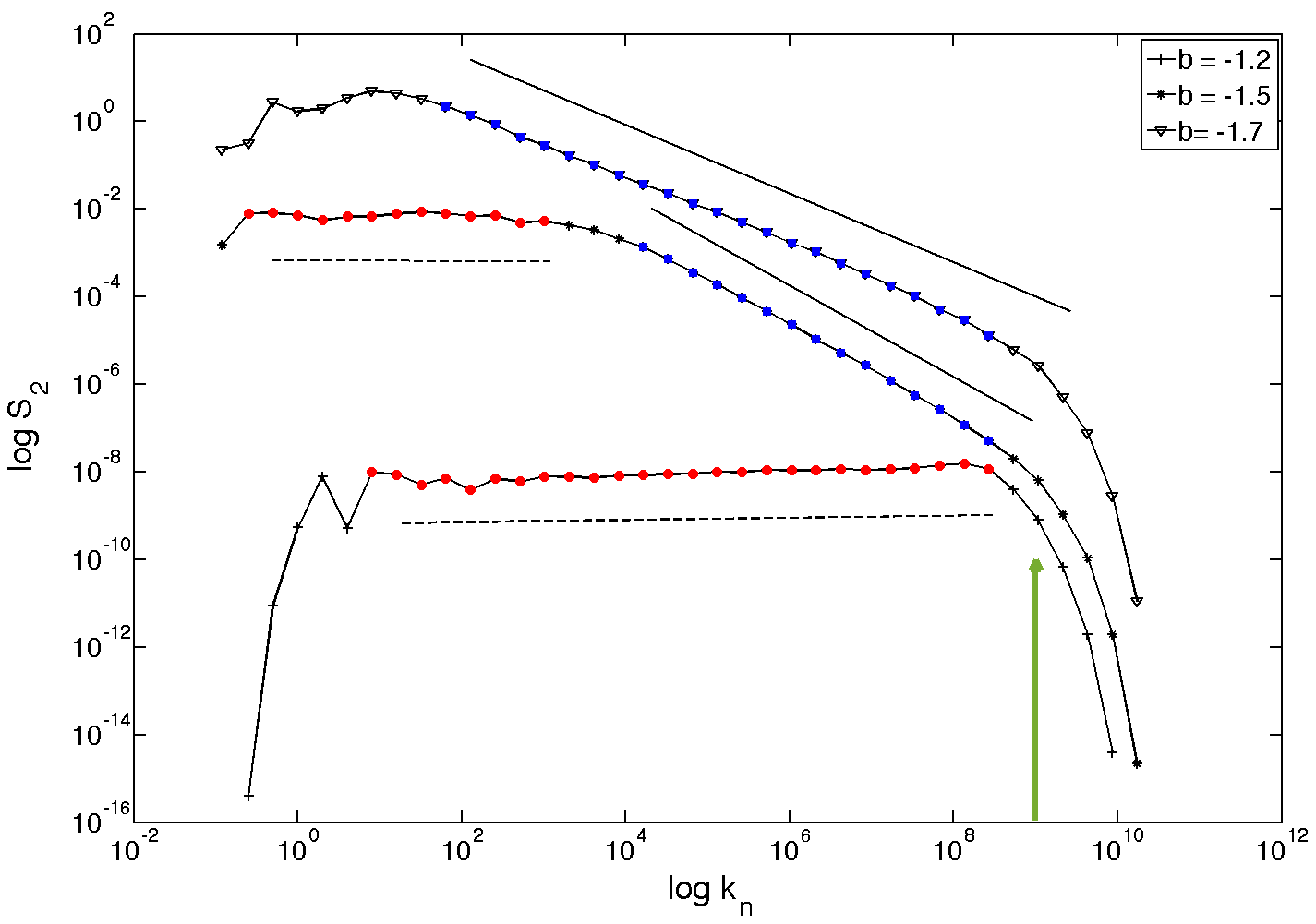
Figure 1: (color online) Representative log-log plots of the second-order equal-time structure functions $S_{2}$ versus $k_{n}$ from run R1 ($N=43$) for $b=-1.2$ (lowest curve), $b=-1.5$ (middle curve), and $b=-1.7$ (top curve). The forcing scale is indicated by the green vertical arrow. For the largest value of $b$ we see that the scaling regime is a plateau (energy equipartition), shown by the red circles and indicated by the horizontal, dashed line; for the smallest value of $b$, we see a clear power-law scaling, with a non-zero exponent (enstrophy equipartition), as shown by the blue triangles and the thick black line as a guide to the eye. For an intermediate value of $b=-1.5$, there are clearly two scaling regimes, namely the flat plateau (shown by the red circles and the dashed line) and a second power-law with a non-zero scaling exponent (shown by the blue triangles and the thick black line). The curves have been shifted arbitrarily for clarity of presentation. A summary of the various exponents and their dependence on $b$ is shown in Fig. 2.

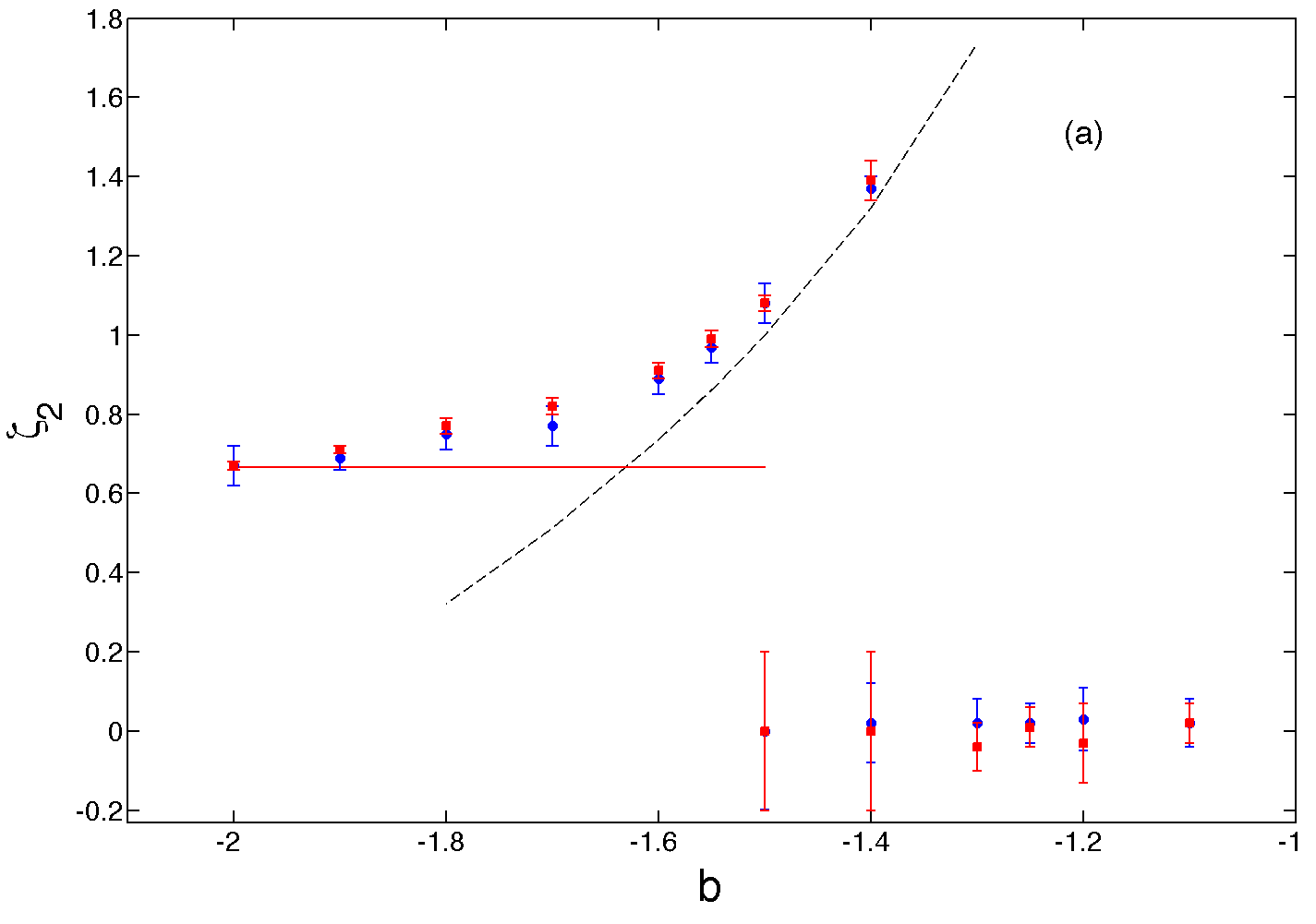
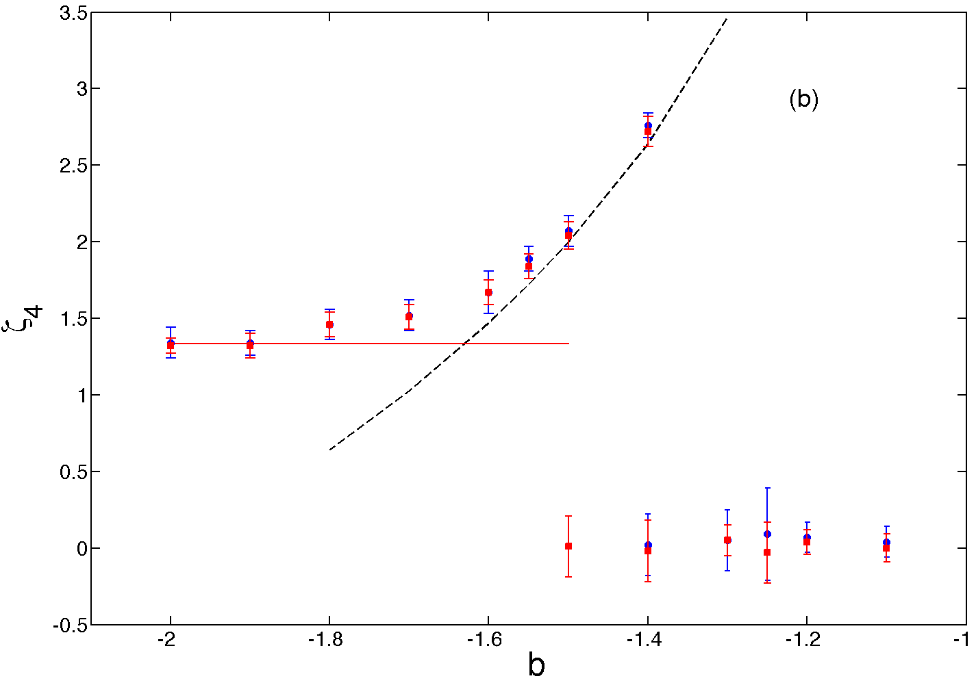
Figure 2: (color online) Equal-time exponents (a) $\zeta_{2}$ and (b) $\zeta_{4}$ as a function of the parameter $b$ from our numerical simulations R1 and R2 of the SABRA model. The various exponents are extracted from log-log plots of the equal-time structure functions as illustrated in Fig. 1. The lower branch correspond to an energy equipartition regime, yielding an exponent $\zeta_{2}=\zeta_{4}=0$ (within error-bars) disappear close to the conjectured critical value $b_{c}$. The upper branch correspond to an enstrophy equipartition regime before converging to the turbulent, Kolmogorov-like solution $\zeta_{2}=2/3$ and $\zeta_{4}=4/3$ (indicated by the horizontal red dot-dashed line in panel). The black, dashed line in panel denotes the exponent predicted from the enstrophy partition regime, namely $\zeta_{2}=\alpha=-\log_{\lambda}|-b-1|$ and $\zeta_{4}=2\zeta_{2}$ for $b>b_{c}$ and for shells larger than $n_{c}$ but smaller than $n_{f}$. We note that, within error-bars, the measured exponents are slightly higher than those obtained theoretically and two-dimensional, turbulent behaviour is only approached asymptotically as $b\to-2$. The exponents obtained from the two sets of simulations, shown as blue circles (R1) and red squares (R2) are in agreement with each other within error-bars.

In Ref. gilbert2002 , the authors showed through a mixture of numerics and theory that the as a function of $b$ the solution of the SABRA model shows a phase diagram with not only the inverse and direct cascade regimes, on either side of the forcing shell $n_{f}$, but also energy and enstrophy equipartition phases on either side of a cross-over shell number (which itself is a function $b$) $n_{c}<n_{f}$ with a phase boundary separating which disappears at $b=b_{c}=-a(1+\lambda^{-2/3})\approx-1.63$. For values $-2<b<b_{c}$, such equilibrium solutions disappear leaving only the dual cascade picture typical of two-dimensional turbulence. It is this rich phase diagram which makes the two-dimensional SABRA model an ideal candidate to study the dynamics in the interplay between turbulence (cascade) and fluxless solutions. In this paper, we revisit the two-dimensional SABRA model and systematically study its statics and dynamics for the full range of $-2<b<-1$.

We perform two different sets of simulations (runs R1 and R2) of Eq. (1); in each case we use 11 different values of $-2<b<-1$ with the total number of shells $N=43$ (R1) and $N=28$ (R2). We use, in addition to the normal viscosity, a hypo-viscous term $\mu k_{n}^{-2}$ to drain the energy at lower shell numbers which accumulate because of inverse cascade  foot1 . We use initial conditions $u_{n}^{0}=k_{n}^{1/2}e^{\imath\vartheta_{n}},$ for $n=1,2$, and $u_{n}^{0}=k_{n}^{1/2}e^{{-k_{n}}^{2}}e^{\imath\vartheta_{n}},$ for $3\leq n\leq N$; $\vartheta_{n}$ is a random angle distributed uniformly between $0$ and $2\pi$. We drive the system to steady state by using a deterministic forcing (a) $f=(1+\imath)\times 5\times 10^{-3}$ on shell $n_{f}=22$ (R2) and (b) $f=(1+\imath)\times 8\times 10^{-3}$ on shell $n_{f}=34$ (R1). We use a slaved, Adams-Bashforth scheme pisarenko ; dhar to integrate Eq. (1) by using a time step (a) $\delta t=10^{-4}$, $\nu=10^{-7}$, and $\mu=10^{-2}$ (R2) and (b) $\delta t=10^{-7}$, $\nu=10^{-14}$, and $\mu=3\times 10^{-4}$ (R1). Given the delicate measurements, it is important to rule out any finite-size (in the scaling range) effects; hence we use these two different-sized simulations and find our results from R1 and R2, which we report below, to agree with each other within error-bars.

We begin with the $p$-th order, equal-time structure function and the associated equal-time exponent $\zeta_{p}$. For the shell model this is defined via

$$S_{p}(k_{n})\equiv\left\langle[u_{n}(t)u^{\ast}_{n}(t)]^{p/2}\right\rangle\sim k_{n}^{-\zeta_{p}},$$ (4)

where $\left\langle\cdot\right\rangle$ denotes an average over time in the steady state.

We compute the $p$-th order structure function (4) by averaging, in the steady state, over a time window $\Delta t\gg 1$. We choose 50 such statistically independent time windows and thence obtain 50 values of the equal-time scaling exponents. We quote the mean of these exponents as $\zeta_{p}$ and their standard deviation is a measure of the error-bar on them.

For the two-dimensional SABRA model, for $b>b_{c}$ and $n<n_{f}$, Ditlevsen and Mogensen  mogensen conjectured that the second-order structure function should show two scaling regimes with different scaling exponents. Thus for lower wavenumber $\zeta_{2}=0$ for $n<n_{c}$ due to energy equipartition and at higher wavenumbers $\zeta_{2}=\alpha$ for $n_{c}<n<n_{f}$ because of enstrophy equipartition. On the other hand, for $b<b_{c}$, similar arguments  gilbert2002 leads one to the conclusion that a single scaling range emerges with $\zeta_{2}=2/3$ for $n<n_{f}$ because of the inverse cascade of two-dimensional turbulence.

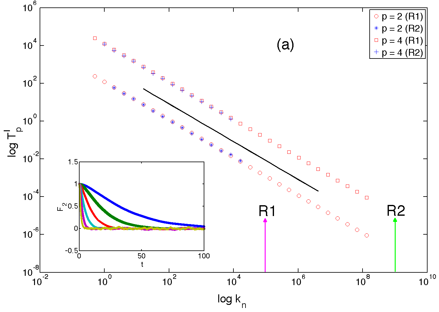
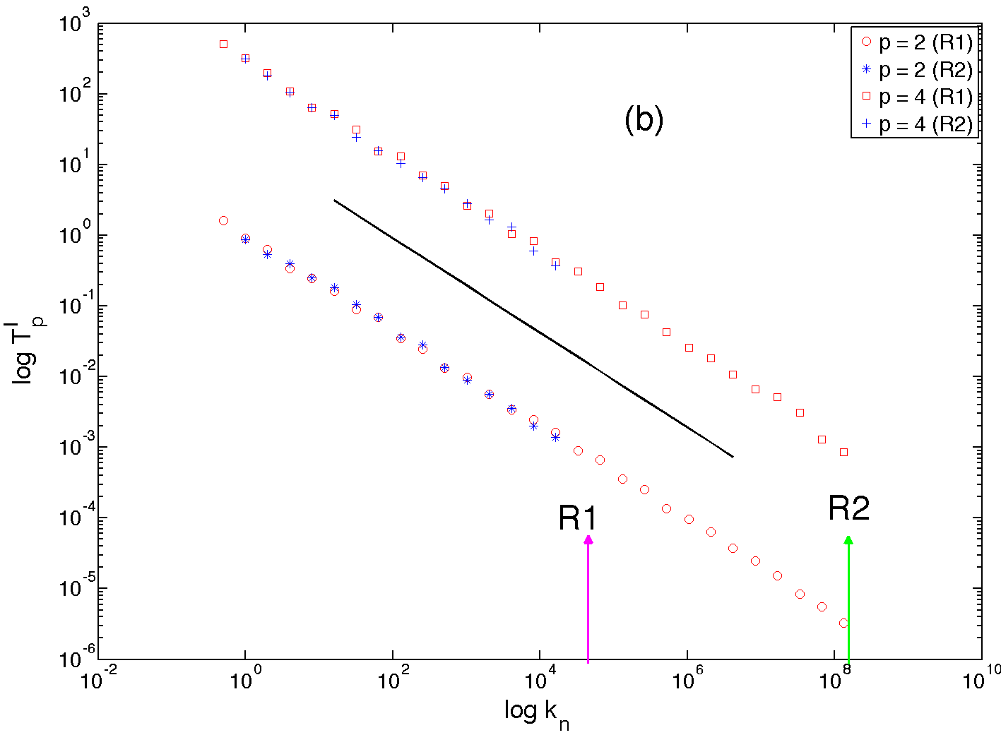
Figure 3: (color online) Representative log-log plots, from runs R1 (red $\circ$ and $\square$) and R2 (blue * and +), of the second and fourth-order integral time scales versus $k_{n}$, for extremal values of $b$, namely (a) $b=-1.2$ and (b) $b=-1.9$. The black, dashed line corresponds to our theoretical prediction in the (a) energy equipartition ($k_{n}^{-1}$) and (b) turbulent, Kolmogorov-like ($k_{n}^{-2/3}$) regimes. The upper set of curves in both panels are for $T^{I}_{4}$ and the lower set of curves for $T^{I}_{2}$. The forcing scales are indicated by the vertical pink and green arrows as labelled in the figure. In the inset of panel (a), we show a representative plot of the time-dependent, second-order structure function $F_{2}$, from where the time-scales are extracted, for several different wavenumbers (inner curves for the larger shell numbers and outer ones for the smaller) as an inset in panel (a). The transition from the equipartition regimes to the turbulent ones is illustrated in Fig. 4.

In Fig. 1 we show representative plots of the second-order, equal-time structure function for different values of $b$. For values of $b>b_{c}$, we find a single plateau ($\zeta_{2}=0$) shown by red circles consistent with earlier predictions. For $b<b_{c}$, a different scaling range, shown with blue triangles, with a power-law exponent $\zeta_{2}\neq 0$. For values of $b$ close to and around the critical $b_{c}$, we find the existence of both these scaling ranges as is clearly seen in Fig. 1.

It is also useful to keep in mind, that a similar conclusion can be drawn by measuring the fluxes as was shown in Ref. gilbert2002 .

In Fig. 2 we show plots of the exponents (a) $\zeta_{2}$ and (b) $\zeta_{4}$ for 12 different values of $b$ from runs R1 (red squares) and R2 (blue circles). For large values of $-1.3\lesssim b\lesssim-1.0$, the scaling range exhibits only the energy equipartition range ($n_{c}\approx n_{f}$) yielding a single exponent, within error-bars, $\zeta_{2}=0.0$. For lower values $b_{c}\lesssim b\lesssim-1.4$, the second-order structure functions show dual scaling (for $n<n_{f}$): $\zeta_{2}=0$ for $n<n_{c}$ and $\zeta_{2}=\alpha$ for $n_{f}<n<n_{c}$. In Fig. 2(a) we see the two branches in the values of $\zeta_{2}$ in the range $b_{c}\lesssim b\lesssim-1.4$. The lower branch $\zeta_{2}=0$ is consistent with the energy equipartition prediction. The black, dashed line corresponds to enstrophy equipartition $\alpha$: However, we find that the measured exponent $\zeta_{2}$ in the second scaling range although close to the enstrophy equipartition prediction is nevertheless marginally larger than $\alpha$. For values of $b\gtrapprox b_{c}$, the scaling of the energy equipartition disappears leaving only the second scaling regime $\zeta_{2}\approx\alpha$. We finally note that this single branch of $\zeta_{2}$ asymptotes to the value 2/3 (denoted by the red, horizontal dot-dashed line) as $b\to-2$. In Fig. 2(b) we show an analogous plot for the fourth-order exponent $\zeta_{4}$ which shows a behaviour consistent to the one we have discussed for $\zeta_{2}$. For both sets of exponents, it is clear that the measurements for different resolutions are consistent with each other within error-bars.

Let us stress that the behaviour of equal-time exponents as a function of $b$ has been discussed before mogensen ; gilbert2002 ; ditlevsenbook . However, our systematic study does throw-up a few surprises which we cannot refrain from commenting upon before we turn our attention to the dynamics of such systems. Firstly, our detailed simulations show that the secondary scaling range yields and exponent which, within error-bars, is marginally larger than $\alpha$ as $b\to b_{c}$. Secondly, and more curiously, the two-dimensional turbulent behaviour – a single scaling range for $n<n_{f}$ – with $\zeta_{p}=p/3$ is recovered only asymptotically as $b\to-2$.

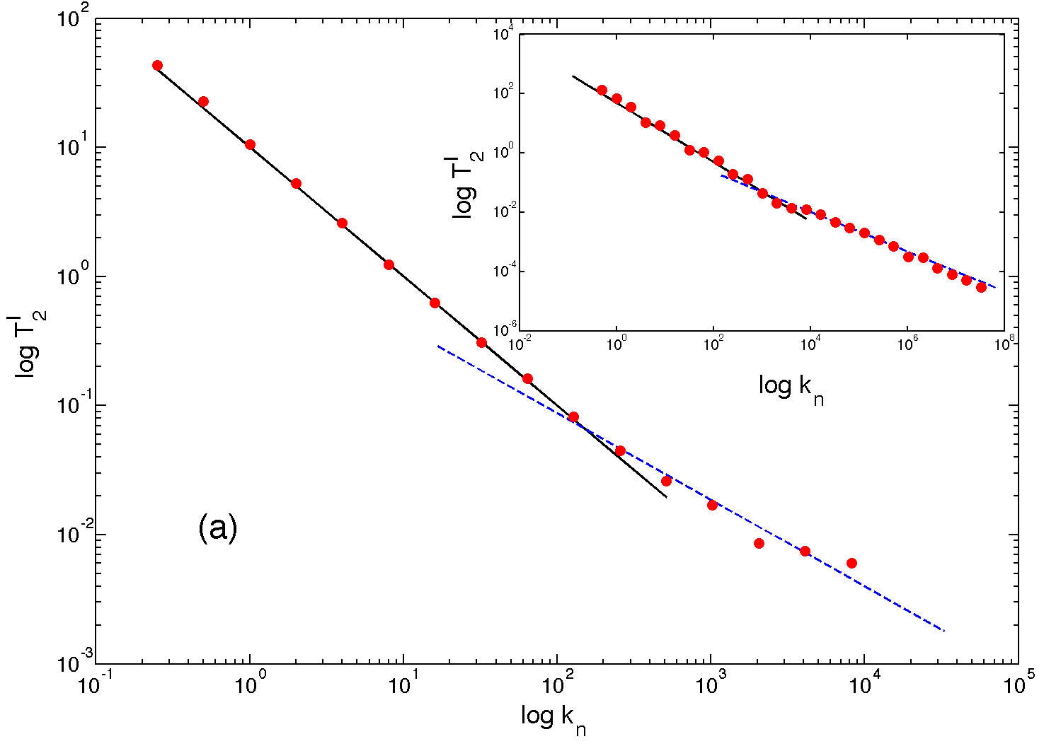
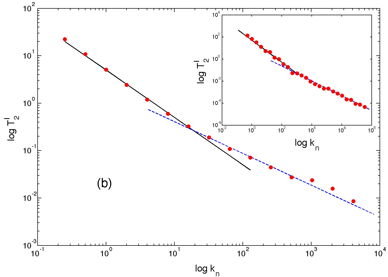
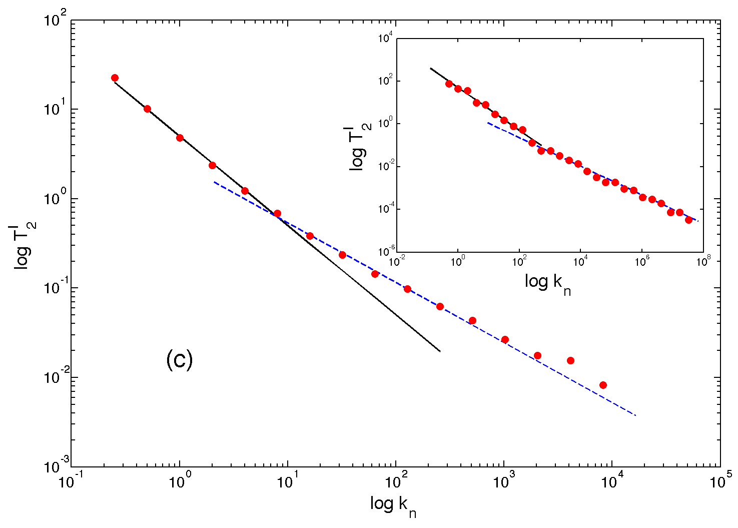
Figure 4: (color online) Representative log-log plots, from runs R2 and R1 (in the insets), of the second-order integral time scale $T_{2}$ versus the wavenumber $k_{n}$ for (a) $b=-1.4$, (b) $b=-1.55$, and (c) $b=-1.7$. In panels (a) and (b), the black, dashed line corresponds to our theoretical prediction, from the energy equipartition arguments, of $k_{n}^{-1}$ ($z_{2}=z_{4}=1$) and the blue, dashed line shows a scaling $k_{n}^{-\alpha/2-1}$ predicted from an enstrophy equipartition solution. In panel (c), where $b<b_{c}$, the blue, dashed line indicates $k_{n}^{-2/3}$, as we would expect from a Kolmogorov-type, turbulent solution.

We finally turn our attention to the dynamics of such systems, especially near the critical point $b_{c}$. This is most conveniently done by examining the time scales associated with the time-dependent order-$p$ structure function, defined for the shell model as

$$F_{p}(k_{n},t)\equiv\left\langle[u_{n}(t_{0})u^{\ast}_{n}(t_{0}+t)]^{p/2}\right\rangle.$$ (5)

This allows us to extract the integral-time scale mitra04 ; mitra05 ; raynjp ; rayepjb via the time integral

$$T_{p}(k_{n})=\frac{1}{F_{p}|_{t=0}}\int_{0}^{t_{\epsilon}}F_{p}ds$$ (6)

and, thence, via the dynamic scaling Ansatz $T_{p}=k_{n}^{-z_{p}}$ the dynamic exponent $z_{p}$. In this integral the upper limit $t_{\epsilon}$ is taken as the time when the time-dependent structure function for a particular shell (Fig. 3a (inset)) falls below a threshold $\epsilon$; for our calculations we choose $\epsilon=0.6$ but have checked that our results are unchanged for $0.4\leq\epsilon\leq 0.7$.

In Fig. 3 we show the representative plots of the second and fourth-order integral time scales, versus the wavenumber, extracted from time-dependent structure functions (inset of Fig. 3a) for extremal values of the parameter (a) $b=-1.2$ and (b) $b=-1.9$. We see clearly that between these two values the scaling behaviour switches from the equipartition $k_{n}^{-1}$ to the Kolmogorov scaling $k_{n}^{-2/3}$. In order to understand this transition clearly, it is important to examine the integral time-scales for intermediate values of $b$.

In Fig. 4 we show representative, log-log plots of $T_{2}$ vs $k_{n}$ for $n<n_{f}$ for such intermediate values of $b$. We see the clear co-existence of both scaling ranges as shown by the thick black line ($k_{n}^{-1}$) and the broken blue line ($k_{n}^{-2/3}$) threading the data. With decreasing $b$, the second scaling regime starts to dominate and at the cost of the first. The fourth-order structure functions show an identical behaviour and, hence, are not presented for brevity. It is possible to estimate the cross-over scales from such plots and in Fig. 5 we show a plot of the ratio of the cross-over wavenumber to the forcing wavenumber as a function of $b$ (in the intermediate range). Given the discrete and exponential spacing of the shell space, we should keep in mind that such estimates are not likely to be very precise.

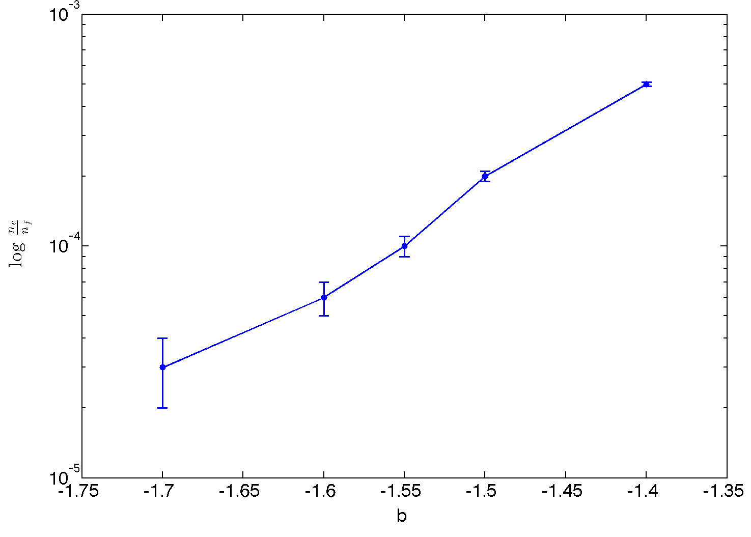
Figure 5: (color online) A plot of the ratio of the estimated cross over shell $n_{c}$ with the forcing shell $n_{f}$ versus the parameter $b$ in the intermediate co-existence region. Within errorbars the curves for runs R1 and R2 agree with each other. We present here results from R1.

Our results for the dynamic exponents is interesting for several reasons. It useful to remind ourselves that, by definition, dynamic exponents in shell models are not affected by sweeping which would trivially yield $z_{2}=1$. Within the multifractal model of three-dimensional turbulence, the dynamic exponents are related to the equal-time ones through a linear bridge relation. Here, however, $z_{2}=1$ is the result of a unique time scale $\tau=1/k_{n}$ because of energy equipartition. Similarly, the second scaling regime is due to the equipartition of the generalised enstrophy which yields, again, a unique time scale $\tau\sim(u_{n}k_{n})^{-1}=k_{n}^{-\alpha/2-1}$. For values of $b$ smaller than the critical value, both these scaling regimes disappear and we end up with a Kolmogorov-like dynamic exponent $z=2/3$ consistent with $\zeta_{2}=2/3$ raynjp . It is useful to draw attention to the fact that the Kolmogorov-like dynamic exponent is, in its numerical value, close to that obtained via an equipartition argument for values of $b$ close to -2. Hence extreme care needs to be taken to disentangle the two effects. It is for these reasons that we performed two sets of simulations with very different extents of the scaling range and found the exponents extracted from both these runs to be in agreement with each other.

In this paper, in the light of recent work on decimated Navier-Stokes turbulence, we revisited the two-dimensional SABRA model to understand, within the simplifications of a shell model, the interplay between cascade and equilibrium solutions. We ought to keep in mind that our work builds on and adds to the previous studies of Refs. mogensen ; gilbert2002 ; ditlevsenbook . In particular, we have explored systematically the phase diagram proposed by Gilbert et al. gilbert2002 and found some surprises. Furthermore we have measured, to our knowledge for the first time, the dynamics of such systems and their associated time scales which, unsurprisingly, are very different from the dynamic multiscaling that we usually associate with fully developed turbulence. Most curiously, our studies show, contrary to previous estimates ditlevsenbook , that the SABRA model mimics two-dimensional turbulence only asymptotically as $b\to-2$. These studies thus reemphasize the hope frisch12 that there might be more in common between statistical mechanics and true two-dimensional turbulence than was thought before. It is left for the future to evaluate the relaxation to equilibrium states and the dynamics close to the critical dimension of Frisch et al. frisch12 in direct numerical simulations of the decimated, two-dimensional Navier-Stokes equation.

The authors are grateful to Anna Pomyalov for many insightful discussions and suggestions. SSR acknowledges the support of the DAE and the DST (India) project ECR/2015/000361. Our simulations were performed on the cluster Mowgli and the work station Goopy at the ICTS-TIFR.

References

- (1) A.N. Kolmogorov, Dokl. Akad. Nauk SSSR 30, 301 (1941); A.N. Kolmogorov, Dokl. Akad. Nauk SSSR 31, 538 (1941).
- (2) U. Frisch, Turbulence: The Legacy of A.N. Kolmogorov (Cambridge University, Cambridge, UK, 1996).
- (3) G. Falkovich, K. Gawedzki and M. Vergassola, Rev. Mod. Phys. 73, 913 (2001).
- (4) R. Pandit, P. Perlekar, and S.S. Ray, Pramana 73, 157 (2009).
- (5) E. Hopf, Comm. Pure Appl. Math. 3, 201 (1950).
- (6) T. D. Lee, Q. J. Appl. Math. 10 (1952). H.K. Moffatt and K.S.R. Sreenivasan, eds., Cambridge University Press, Cambridge, (2010).
- (7) C. Cichowlas, P. Bonaïti, F. Debbash, and M. Brachet, Phys. Rev. Lett. 95, 264502 (2005).
- (8) S. S. Ray, U. Frisch, S. Nazarenko, and T. Matsumoto, Phys. Rev. E 84, 16301 (2011).
- (9) D. Banerjee and S. S. Ray, Phys. Rev. E 90, 041001(R) (2014).
- (10) S. S. Ray, in Persp. in Nonlinear Dynamics, Pramana - J. of Phys. 84, 395, (2015).
- (11) D. Venkataraman and S. S. Ray, Proc. Royal Soc. A 473, 20160585 (2017).
- (12) U. Frisch, S. Kurien, R. Pandit, W. Pauls, S. S. Ray, A. Wirth, and J-Z Zhu, Phys. Rev. Lett. 101, 144501 (2008).
- (13) U. Frisch, S. S. Ray, G. Sahoo, D. Banerjee, and R. Pandit, Phys. Rev. Lett., 110, 64501 (2013).
- (14) W. Dobler, N.E.L. Haugen, T.A. Yousef and A. Brandenburg, Phys. Rev. E, 68, 026304 (2003); Z.-S. She, G. Doolen, R.H. Kraichnan, and S.A. Orszag, Phys. Rev. Lett., 70, 3251 (1993); P.K. Yeung and Y. Zhou, Phys. Rev. E, 56, 1746 (1997); T. Gotoh, D. Fukayama, and T. Nakano, Phys. Fluids, 14, 1065 (2002); M.K. Verma and D.A. Donzis, J. Phys. A: Math. Theor., 40, 4401 (2007); P.D. Mininni, A. Alexakis, and A. Pouquet, Phys. Rev. E, 77, 036306 (2008). Y. Kaneda, et al., Phys. Fluids, 15, L21 (2003); T. Isihara, T. Gotoh, and Y. Kaneda Annu. Rev. Fluid Mech., 41, 165 (2009); S. Kurien, M.A. Taylor, and T. Matsumoto, Phys. Rev. E, 69, 066313 (2004); D.A. Donzis and K.R. Sreenivasan J. Fluid Mech., 657, 171 (2010); H.K. Pak, W.I. Goldburg, A. Sirivat, Fluid Dynamics Research, 8, 19 (1991); Z.-S. She and E. Jackson, Phys. Fluids A, 5, 1526 (1993); S.G. Saddoughi and S.V. Veeravalli, J. Fluid Mech., 268, 333 (1994); G. Falkovich, Phys. Fluids, 6, 1411 (1994); L. Sirovich, L. Smith, and V. Yakhot, Phys. Rev. Lett., 72, 344, (1994).
- (15) V. L’vov, A. Pomyalov and I. Procaccia, Phys. Rev. Lett. 89, 064501 (2002).
- (16) U. Frisch, A. Pomyalov, I. Procaccia, and S. S. Ray, Phys. Rev. Lett. 108, 074501 (2012).
- (17) A. S. Lanotte, R. Benzi, S. K. Malapaka, F. Toschi, and L. Biferale, Phys. Rev. Lett. 115, 264502 (2015).
- (18) A. S. Lanotte, S. K. Malapaka, L. Biferale, Eur. Phys. J. E 39, 49 (2016).
- (19) M. Buzzicotti, A. Bhatnagar, L. Biferale, A. S. Lanotte, S. S. Ray, New J. of Phys. 18, 113047 (2016).
- (20) M. Buzzicotti, L. Biferale, U. Frisch, and S. S. Ray, Phys. Rev. E 93, 033109 (2016).
- (21) D. Mitra and R. Pandit, Phys. Rev. Lett. 93, 024501 (2004).
- (22) D. Mitra and R. Pandit, Phys. Rev. Lett. 95, 144501 (2005).
- (23) R. Pandit, S. S. Ray and D. Mitra, Eur. Phys. J. B 64, 463 (2008).
- (24) S. S. Ray, D. Mitra and R. Pandit, New J. Phys. 10, 033003 (2008).
- (25) L. Biferale, E. Calzavarini, and F. Toschi, Phys. Fluids 23, 085107 (2011).
- (26) S. S. Ray, D. Mitra, P. Perlekar, and R. Pandit, Phys. Rev. Lett. 107, 184503 (2011).
- (27) G. Parisi and U. Frisch in Turbulence and Predictability of Geophysical Fluid Dynamics, eds. M. Ghil, R. Benzi, and G. Parisi (North-Holland, Amsterdam, 1985) p 84.
- (28) P. D. Ditlevsen and I. A. Mogensen, Phys. Rev. E 53, 4785 (1996).
- (29) T. Gilbert, V. S. L’vov, A. Pomyalov, and I. Procaccia, Phys. Rev. Lett. 89 074501 (2002).
- (30) L. Biferale, Annu. Rev. Fluid Mech. 35, 441 (2003)
- (31) V.S. L’vov, E.Podivilov, A. Pomyalov, I. Procaccia, and D. Vandembroucq, Phy. Rev. 58, 1811 (1998)
- (32) E. B. Gledzer, Dokl. Akad. Nauk SSSR 209, 1046 (1973) [Sov. Phys. Dokl. 18, 216 (1973)]; M. Yamada and K. Ohkitani, Phys. Rev. Lett. 60, 983 (1988).
- (33) P. D. Ditlevsen, Turbulence and Shell Models (Cambridge University, Cambridge, UK, 2010).
- (34) T. Bohr, M. H. Jensen, G. Paladin and A. Vulpiani, Dynamical systems approach to turbulence (Cambridge University Press, Cambridge, UK, 1998).
- (35) We note that this is in the spirit of standard DNSs of two-dimensional Navier-Stokes equation rayprl11 ; perlekar11 where a friction term is added to mimic air-drag-induced friction which prevents accumulation of energy at the largest scales.
- (36) P. Perlekar, S. S. Ray, D. Mitra, and R. Pandit, Phys. Rev. Lett. 106, 054501 (2011).
- (37) D. Pisarenko, L. Biferale, D. Courvoisier, U. Frisch, and M. Vergassola, Phys. Fluids A 5, 2533 (1993).
- (38) S. Dhar, A. Sain, and R. Pandit, Phys. Rev. Lett. 78, 2964 (1997).