Abstract

In this note we show how a initial value problem for a relaxation process governed by a differential equation of non-integer order with a constant coefficient may be equivalent to that of a differential equation of the first order with a varying coefficient. This equivalence is shown for the simple fractional relaxation equation that points out the relevance of the Mittag-Leffler function in fractional calculus. This simple argument may lead to the equivalence of more general processes governed by evolution equations of fractional order with constant coefficients to processes governed by differential equations of integer order but with varying coefficients. Our main motivation is to solicit the researchers to extend this approach to other areas of applied science in order to have a more deep knowledge of certain phenomena, both deterministic and stochastic ones, nowadays investigated with the techniques of the fractional calculus.

Keywords: Caputo fractional derivatives, Mittag–Leffler functions, anomalous relaxation. MSC: 26A33, 33E12, 34A08, 34C26. Published on line 9 January 2018: MATHEMATICS Vol. 6 (2018) Paper 8, 5pp. DOI: 10.3390/math6010008

1 Introduction

Let us consider the following relaxation equation

$$\frac{d\Psi}{dt}=-r(t)\,\Psi(t)\,,\quad t\geq 0\,,$$ (1)

subjected to the initial condition, for the sake of simplicity,

$$\Psi(0^{+})=1\,,$$ (2)

where $\Psi(t)$ and $r(t)$ are positive functions, sufficiently well-behaved for $t\geq 0$. In Eq. (1) $\Psi(t)$ denotes a non-dimensional field variable and $r(t)$ the varying relaxation coefficient.

The solution of the above initial value problem reads

$$\Psi(t)=\hbox{exp}[-R(t)]\,,\quad R(t)=\int_{0}^{t}\!r(t^{\prime})\,dt^{\prime}>0\,.$$ (3)

It is easy to recognize from re-arranging Eq. (1) that for $t\geq 0$

$$r(t)=-\frac{\Phi(t)}{\Psi(t)}\,,\quad\Phi(t)=\Psi^{(1)}(t)=\frac{d\Psi}{dt}(t)\,.$$ (4)

The solution (3) can be derived by solving the initial value problem by separation of variables

$$\int_{1}^{\Psi(t)}\!\frac{d\Psi(t^{\prime})}{\Psi(t^{\prime})}=\int_{0}^{t}\!\frac{\Phi(t^{\prime})}{\Psi(t^{\prime})}\,dt^{\prime}=-\int_{0}^{t}\!r(t^{\prime})\,dt^{\prime}=R(t).$$ (5)

From Eq, (3) we also note that

$$R(t)=-\log[\Psi(t)]\,.$$ (6)

As a matter of fact, we have shown well-known results that will be relevant for the next Sections.

2 Mittag-Leffler function as solution of the fractional relaxation process

Let us now consider the following initial value problem for the so-called fractional relaxation process

$$\begin{cases}{}_{*}D_{t}^{\alpha}\Psi_{\alpha}((t)=-\Psi_{\alpha}(t),&t\geq 0,\\ \Psi_{\alpha}(0^{+})=1,\end{cases}$$ (7)

with $\alpha\in(0,1]$. Above we have labeled the field variable with $\Psi_{\alpha}$ to point out is dependence on $\alpha$ and the considered the Caputo fractional derivative, defined as:

$${}_{*}D_{t}^{\alpha}\Psi_{\alpha}(t)=\begin{cases}{\displaystyle\frac{1}{\Gamma(1-\alpha)}\int_{0}^{t}\frac{\Psi_{\alpha}^{(1)}(t^{\prime})}{(t-t^{\prime})^{\alpha}}\,dt^{\prime}},&0<\alpha<1,\\ \\ {\displaystyle\frac{d}{dt}\Psi_{\alpha}(t)}\,,&\alpha=1.\end{cases}$$ (8)

As found in many treatises of fractional calculus, and in particular in the 2007 survey paper by Mainardi and Gorenflo [2] to which the interested reader is referred for details and additional references, the solution of the fractional relaxation problem (7) can be obtained by using the technique of the Laplace transform in terms of the Mittag-Leffler function. Indeed, we get in an obvious notation by applying the Laplace transform to Eq. (7)

$$s^{\alpha}\widetilde{\Psi}_{\alpha}(s)-s^{\alpha-1}=-\widetilde{\Psi}_{\alpha}(s),\quad\hbox{hence}\quad\widetilde{\Psi}_{\alpha}(s)=\frac{s^{\alpha-1}}{s^{\alpha}+1},$$ (9)

so that

$$\Psi_{\alpha}(t)=E_{\alpha}(-\ t^{\alpha})=\sum_{0}^{\infty}(-1)^{n}\frac{t^{\alpha n}}{\Gamma(\alpha n+1)}\,.$$ (10)

For more details on the Mittag-Leffler function we refer to the recent treatise by Gorenflo et al. [1]. Here, for readers’ convenience, we report the plots of the solution (10) for some values of the parameter $\alpha\in(0,1]$.

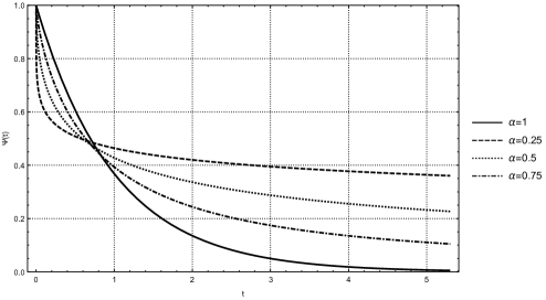
Figure 1: Plots of the Mittag-Leffler function $\Psi_{\alpha}(t)$ for $\alpha=0.25,0.50.0.75,1$ versus $t\in[0.5]$.

It can be noticed that for $\alpha\to 1^{-}$ the solution of the initial value problem reduces to the exponential function $\hbox{exp}(-t)$ with a singular limit for $t\to\infty$ because of the asymptotic representation for $\alpha\in(0,1)$,

$$E_{\alpha}(-\ t^{\alpha})\sim\frac{t^{-\alpha}}{\Gamma(-\alpha+1)}\,,\quad t\to\infty\,.$$ (11)

Now it is time to carry out the comparison between the two initial value problems described by Eqs. (1), (7) with their corresponding solutions (3), (10). It is clear that we must consider the derivative of the Mittag-Leffler function in (10), namely

$$\Phi_{\alpha}(t)=\frac{d}{dt}\Psi_{\alpha}(t)=\frac{d}{dt}E_{\alpha}(-t^{\alpha})=-t^{\alpha-1}\,E_{\alpha,\alpha}(-t^{\alpha})\,.$$ (12)

In Fig 2 we show the plots of positive function $-\Phi_{\alpha}(t)$ for some values of $\alpha\in(0,1]$.

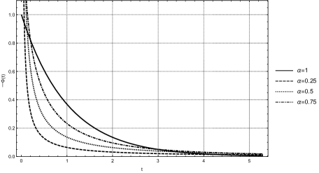
Figure 2: Plots of the positive function $-\Phi_{\alpha}(t)$ for $\alpha=0.25,0.50.0.75,1$ versus $t\in[0.5]$.

The above discussion leads to the varying relaxation coefficient of the equivalent ordinary relaxation process:

$$r_{\alpha}(t)=-\frac{\Phi_{\alpha}(t)}{\Psi_{\alpha}(t)}\Longrightarrow r_{\alpha}(t)=\frac{t^{\alpha-1}E_{\alpha,\alpha}(-t^{\alpha})}{E_{\alpha}(-t^{\alpha})}.$$ (13)

Fig. 3 depicts the plots of $r_{\alpha}(t)$ for some rational values of $\alpha$, including the standard case $\alpha=1$, in which the ratio reduces to the constant 1.

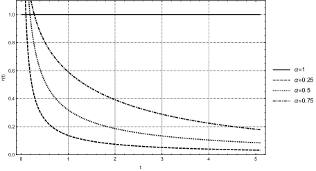
Figure 3: Plots of the ratio $r_{\alpha}(t)$ for $\alpha=0.25,0.50,0.75,1$ versus $t\in[0.5]$.

We conclude by plotting the function $R_{\alpha}(t)=-\log[\Psi_{\alpha}(t)]$ for some values of the parameter $\alpha\in(0,1]$.

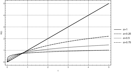
Figure 4: Plots of $R_{\alpha}(t)$ for $\alpha=0.25,0.50,0.75,1$ versus $t\in[0.5]$.

3 Conclusions

In this note we have shown how the fractional relaxation process governed by a fractional differential equation with a constant coefficient is equivalent to a relaxation process governed by an ordinary differential equation with a varying coefficient. These considerations provide a different look at this fractional process over all for experimentalists who can measure the varying relaxation coefficient versus time. We are convinced that it is possible to adapt the above reasoning to other fractional processes, including anomalous relaxation in viscoelastic and dielectric media and anomalous diffusion in complex systems. This extension is left to perceptive readers who can explore these possibilities.
Last but not the least, we do not claim to be original in using the above analogy in view of the great simplicity of the argument: for example, a similar procedure has recently been used by Sandev et al. [3] in dealing with the fractional Schrödinger equation.

References

- [1] Gorenflo, R., Kilbas, A.A., Mainardi, F., Rogosin, S., Mittag-Leffler Functions. Related Topics and Applications, Springer, Berlin (2014).
- [2] Mainardi, F., Gorenflo, R., Time-fractional derivatives in relaxation processes: a tutorial survey, Fract. Calc. Appl. Anal. 10, 269–308 (2007). [E-print: http://arxiv.org/abs/0801.4914]
- [3] Sandev, T., Petreska, I., Lenzi, E.K., Effective potential from the generalized time-dependent Schrödinger equation, Mathematics 4, 59–68 (2016). doi:10.3390/math4040059.