Optical Transparency in an effective model for Graphene

Abstract

Motivated by experiments confirming that the optical transparency of graphene is defined through the fine structure constant and that it could be fully explained within the relativistic Dirac fermions in 2D picture, in this article we investigate how this property is affected by next-to-nearest neighbor coupling in the low-energy continuum description of graphene. A detailed calculation within the linear response regime allows us to conclude that, somewhat surprisingly, the zero-frequency limit of the optical conductivity that determines the transparency remains robust up to this correction.

Keywords: Quantum Mechanics, Graphene, Quantum Hall effect.

1 Introduction

Graphene is a two-dimensional allotrope of carbon, arranged as a honeycomb lattice with a $C_{3v}\otimes Z_{2}$ symmetry [1] that determines its remarkable physical properties [2, 3, 4, 5]. In particular, the electronic spectrum arising from an atomistic tight-binding model displays two non-equivalent points $K_{+},\,K_{-}$ where the conduction and valence bands touch, and in whose vicinity the dispersion relation is approximately linear. This leads to an effective, low-energy continuum model where the electronic properties of the material are well captured by those of relativistic Dirac fermions in 2D. Among the plethora of physical consequences of this fact that have been already predicted and measured [2, 3, 4, 5, 6, 7, 8], we noticed an interesting experiment that measures the optical transparency of single and few-layer graphene [9]. The transparency is a physical property that is determined by the optical conductivity, i.e. the linear response to an electromagnetic field, in the zero-frequency limit. A variety of experiments confirm [9, 10, 11, 12, 13] that the measured transmittance is indeed compatible with the effective single-particle model of relativistic Dirac fermions in graphene. A number of different theoretical works have exploited this fact to calculate the light absorption rate in graphene from a “relativistic” quantum electrodynamics perspective [14, 15, 16, 17, 18, 19, 20, 21, 22]. An interesting question that remains open is up to what extent this effective model is valid in the representation of this optical property, since it arises from a tight-binding microscopic atomistic model that involves only the nearest neighbor hopping. In this article, we decided to explore what is the contribution to the optical conductivity arising from the next-to-nearest neighbors coupling in the atomistic Hamiltonian, included as a quadratic correction to the kinetic energy operator within the continuum effective model for graphene. Such a model has been considered in Ref. [23] to fully account for the Anomalous Integer Quantum Hall Effect in this material and the underlying wave equation is referred to in literature as Second Order Dirac Equation [24]. For our purposes, let us recall that within the linear response theory, general Kubo relations allow to express the transport coefficients in terms of retarded correlators [25], that for a pair of observables $\hat{O}_{1}$, $\hat{O}_{2}$ are defined by ($\zeta=\pm$ for Bosons and Fermions, respectively)

$$C_{O_{1},O_{2}}^{R}(t-t^{\prime}) = -i\theta(t-t^{\prime})\langle[\hat{O}_{1}(t),\hat{O}_{2}(t^{\prime})]_{-\zeta}\rangle$$ (1.1)

$$= -i\theta(t-t^{\prime})\langle\hat{O}_{1}(t)\hat{O}_{2}(t^{\prime})\rangle-i\theta(t-t^{\prime})\zeta\langle\hat{O}_{2}(t^{\prime})\hat{O}_{1}(t)\rangle.$$

These retarded correlators differ from the usual time-ordered ones that, by construction, are obtained via functional differentiation of the standard generating functional constructed form a path-integral formulation in quantum field theory. This rather technical inconvenience can be overcome by connecting the different propagators using a Lehmann representation, or alternatively to work in the Matsubara formalism at finite temperature and use analytic continuation a posteriori [25]. There is however a third, and more direct alternative, which is to express the generating functional in the contour time path (CTP), also known as Keldysh formalism in the condensed matter literature [26, 27]. In this work, we choose the CTP formalism to explicitly calculate the polarization tensor as a retarded correlator of the current operators, which provides the correct definition of the optical conductivity within linear response theory. With these ideas in mind, we have organized the remaining of this article as follows: In Sect. 2, we present the details of the model. In Sect. 3 we present the Keldysh formalism to calculate the current-current correlator and in Sect. 4 we obtain the optical conductivity from the vacuum polarization tensor. We discuss our findings in Sect. 5. Some calculational details are presented in an Appendix.

2 Lagrangian, conserved current and generating functional

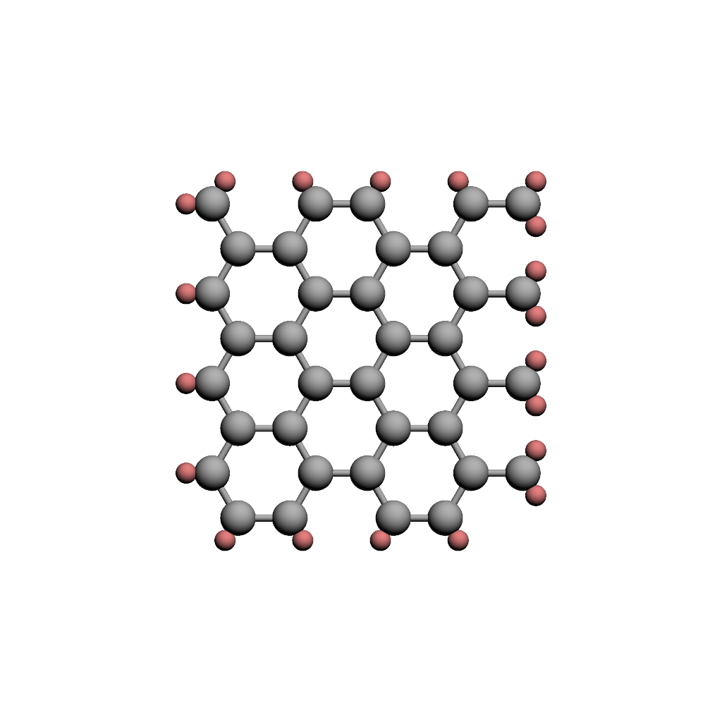
Figure 1: (Color online) Sketch of the crystal structure of graphene. The honeycomb array is described in terms of two overlapping triangular sublattices.

Graphene consist in one atom thick membrane of tightly packed carbon atoms in a honeycomb array. Its crystal structure, sketched in Fig. 1, is described in terms of two overlapping triangular (Bravais) sublattices so that for a given atom belonging to any of these sublattices, its nearest neighbors belong to the second sublattice, the next-to-nearest neighbors to the original sublattice and so on. The band structure at the next-to-nearest approximation is of the form

$$E_{\pm}(\mathbf{k})=\pm t\sqrt{f(\mathbf{k})}-t^{\prime}[f(\mathbf{k})-3],$$ (2.1)

where $t$ and $t^{\prime}$ are the nearest and next-to-nearest hopping parameters and

$$f(\mathbf{k})=3+4\cos\left(\frac{3k_{x}a}{2}\right)\cos\left(\frac{\sqrt{3}k_{y}a}{2}\right)+2\cos(\sqrt{3}k_{y}a)\;,$$ (2.2)

where $a\simeq 1.42\AA$ is the interatomic distance. The points $K_{+}$ and $K_{-}$ at which $f(K_{\pm})=0$ define the so-called Dirac points. Around $K_{+}$,

$$E_{\pm}(\mathbf{k}+K_{+})=\pm t\left[\frac{3}{2}a|\mathbf{k}|-\frac{3}{8}a^{2}\mathbf{k}^{2}\sin(3\vartheta)\right]+t^{\prime}\left[-\frac{9}{4}a^{3}\mathbf{k}^{2}+3\right]+{\cal O}(|\mathbf{k}|^{3})\;,$$ (2.3)

with $\tan(\vartheta)=k_{y}/k_{x}$. Around $K_{-}$ one merely has to replace $\vartheta\to-\vartheta$ in Eq. (2.3). The isotropic portion of this model was first considered in Ref. [23] as a natural framework to explain the Anomalous Integer Quantum Hall Effect in graphene. The anisotropic term in that work was treated perturbatively and shown not to contribute to the energy spectrum at first order. In the presence of electromagnetic interactions, the model is described by the Lagrangian [23]

$$\mathcal{L} := \frac{i}{2}\left[\psi^{\dagger}\,\partial_{t}\psi-\partial_{t}\psi^{\dagger}\,\psi\right]+\psi^{\dagger}eA_{0}\psi$$ (2.4)

$$-\frac{1}{2m}\left\{\left[\left(\mathbf{p}-e\mathbf{A}+\theta\boldsymbol{\sigma}\right)\psi\right]^{\dagger}\cdot\left[\left(\mathbf{p}-e\mathbf{A}+\theta\boldsymbol{\sigma}\right)\psi\right]-2\theta^{2}\psi^{\dagger}\psi\right\}$$

$$= \frac{i}{2}\left[\psi^{\dagger}\,\partial_{t}\psi-\partial_{t}\psi^{\dagger}\,\psi\right]-\frac{1}{2m}\left\{\boldsymbol{\nabla}\psi^{\dagger}\cdot\boldsymbol{\nabla}\psi+i\boldsymbol{\nabla}\psi^{\dagger}\cdot\left(-e\mathbf{A}+\theta\boldsymbol{\sigma}\right)\psi-\right.$$

$$\left.-i\psi^{\dagger}\left(-e\mathbf{A}+\theta\boldsymbol{\sigma}\right)\cdot\boldsymbol{\nabla}\psi+\psi^{\dagger}\left[\left(-e\mathbf{A}+\theta\boldsymbol{\sigma}\right)^{2}-2\theta^{2}\right]\psi\right\}\,,$$

where $\theta=mv_{F}$. Here, $\psi^{\dagger}$ and $\psi$ are regarded as independent fields whose equations of motion are derived from the variation of the action with respect to these fields, namely,

$$\frac{\partial\mathcal{L}}{\partial\psi^{\dagger}}-\partial_{t}\left(\frac{\partial\mathcal{L}}{\partial\left(\partial_{t}\psi^{\dagger}\right)}\right)-\boldsymbol{\nabla}\cdot\left(\frac{\partial\mathcal{L}}{\partial\left(\boldsymbol{\nabla}\psi^{\dagger}\right)}\right)$$ (2.5)

$$=i\partial_{t}\psi-\frac{1}{2m}\left[\left(\mathbf{p}-e\mathbf{A}+\theta\boldsymbol{\sigma}\right)^{2}-2\theta^{2}\right]\psi=0\,,$$

and similarly for $\psi$.

The Lagrangian in Eq.(2.4) remains invariant against the local change in the dynamical variables and the external electromagnetic field

$$\begin{array}[]{c}\displaystyle\psi(x)\rightarrow e^{ie\alpha(x)}\psi(x)\quad\Rightarrow\quad\delta\psi(x)=ie\alpha(x)\psi(x)\,,\\ \\ \displaystyle\psi^{\dagger}(x)\rightarrow\psi^{\dagger}(x)e^{-ie\alpha(x)}\quad\Rightarrow\quad\delta\psi^{\dagger}(x)=-ie\alpha(x)\psi^{\dagger}(x)\,,\\ \\ \displaystyle A_{\mu}(x)\rightarrow A_{\mu}(x)+\partial_{\mu}\alpha(x)\,,\end{array}$$ (2.6)

that is, it has a $U(1)$ gauge symmetry. Nœther’s Theorem leads to the existence of the locally conserved current

$$\alpha j^{\mu}:=-\delta\psi^{\dagger}\left(\frac{\partial\mathcal{L}}{\partial\left(\partial_{\mu}\psi^{\dagger}\right)}\right)-\left(\frac{\partial\mathcal{L}}{\partial\left(\partial_{\mu}\psi\right)}\right)\delta\psi\,.$$ (2.7)

The corresponding charge density is

$$j^{0}=e\,\psi^{\dagger}\psi$$ (2.8)

and the current density

$${j^{k}}=\frac{e}{2m}\left\{i\left(\partial_{k}\psi^{\dagger}\,\psi-\psi^{\dagger}\,\partial_{k}\psi\right)+2\psi^{\dagger}\left(-e{A_{k}}+\theta\sigma_{k}\right)\psi\right\}\,.$$ (2.9)

It is straightforward to verify, from the equations of motion, that $j^{\mu}$ is conserved,

$$\partial_{\mu}j^{\mu}=\partial_{t}j^{0}-\boldsymbol{\nabla}\cdot\mathbf{j}=0\,.$$ (2.10)

Notice also that we can write

$$j^{\mu}(x)=\frac{\delta}{\delta A_{\mu}(x)}\int\mathcal{L}(y)\,d^{3}y\,.$$ (2.11)

With these ingredients, we can formulate the corresponding current-current correlator.

3 Generating functional in the Contour Time Path.

We seek to calculate the polarization tensor, defined as a retarded current-current correlator that, in linear response, determines the optical conductivity. For that purpose, we choose to represent the field-theory described in the previous section on the Contour Time Path (CTP) [26, 27]. Let us define the contour $\gamma=\gamma_{-}\oplus\gamma_{+}$, where $\gamma_{-}$ represents the time-ordered branch while $\gamma_{+}$ the anti-time-ordered branch, as depicted in Fig.2. Therefore, we define a contour evolution parameter $\tau\in\gamma$, such that

$$\tau=\left\{\begin{array}[]{cc}t_{-},&\tau\in\gamma_{-}\;,\\ t_{+},&\tau\in\gamma_{+}\;.\end{array}\right.$$ (3.3)

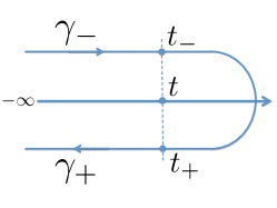
Figure 2: (Color online) The contour $\gamma=\gamma_{+}\oplus\gamma_{-}$ is depicted in the figure. The double folding of the time axis is displayed, by showing that always two points $t_{-}$ and $t_{+}$, located in the time ordered $t_{-}\in\gamma_{-}$ and and anti-time ordered $t_{+}\in\gamma_{+}$ branches of the contour correspond to the same chronological time instant $t$.

Also notice that, as depicted in Fig.2, both $t_{+}$ and $t_{-}$ have a unique correspondence to a given chronological instant of time $t\in{\rm I\!R}$. Correspondingly, for operators and fields defined with their time arguments along the CTP, we have the definitions

$$\psi(\mathbf{x},\tau)=\left\{\begin{array}[]{cc}\psi(\mathbf{x},t_{-})\equiv\psi_{-}(\mathbf{x},t),&\tau\in\gamma_{-}\;,\\ \psi(\mathbf{x},t_{+})\equiv\psi_{+}(\mathbf{x},t),&\tau\in\gamma_{+}\;.\end{array}\right.$$ (3.6)

Then, the generating functional of (current) Green’s functions of this two-dimensional system, defined on the CTP reads

$$Z_{\gamma}[A]=e^{i\Gamma_{\gamma}[A]}:=\int\mathcal{D}\psi^{\dagger}(\mathbf{x},\tau)\mathcal{D}\psi(\mathbf{x},\tau)\,e^{\displaystyle i\int_{\gamma}d\tau\int d^{2}\mathbf{x}\,\mathcal{L}[\psi^{\dagger}(\mathbf{x},\tau),\psi(\mathbf{x},\tau)]}\,,$$ (3.7)

where $\Gamma_{\gamma}[A]$ is the effective contribution to the action for the electromagnetic field. The path-integral on the CTP induces by construction the contour-ordering between the fields, defined by the operation $\mathcal{T}$ between two operators $\hat{O}_{1}(\tau)$ and $\hat{O}_{2}(\tau)$ in the Heisenberg picture ($\zeta=\pm$ for Bosons/Fermions, respectively)

$$\langle\mathcal{T}\hat{O}_{1}(\tau_{1})\hat{O}_{2}(\tau_{2})\rangle = \theta(\tau_{1}-\tau_{2})\langle\hat{O}_{1}(\tau_{1})\hat{O}_{2}(\tau_{2})\rangle$$ (3.8)

$$+\zeta\theta(\tau_{2}-\tau_{1})\langle\hat{O}_{2}(\tau_{2})\hat{O}_{1}(\tau_{1})\rangle.$$

Here, we have defined the contour Heaviside function as

$$\theta(\tau_{1}-\tau_{2})=\left\{\begin{array}[]{cc}1,&\tau_{1}>_{c}\tau_{2}\;,\\ 0,&\tau_{2}>_{c}\tau_{1}\;,\end{array}\right.$$ (3.11)

with the symbol $>_{c}$ indicating the relation “later than in the contour”. In general physical situations where the sources and external fields do not break time-reversal invariance, $\psi_{-}(x,t)=\psi_{+}(x,t)$, and the CTP becomes just a useful trick to express at once all the different correlators. Consider for instance the contour-ordered correlator between two fields,

$$\Delta(\mathbf{x}_{1},\tau_{1};\mathbf{x}_{2},\tau_{2}) \equiv -i\langle\mathcal{T}\psi(\mathbf{x}_{1},\tau_{1})\psi^{\dagger}(\mathbf{x}_{2},\tau_{2})\rangle$$ (3.12)

$$= \theta(\tau_{1}-\tau_{2})(-i)\langle\psi(\mathbf{x}_{1},\tau_{1})\psi^{\dagger}(\mathbf{x}_{2},\tau_{2})\rangle$$

$$+\zeta\theta(\tau_{2}-\tau_{1})(-i)\langle\psi^{\dagger}(\mathbf{x}_{2},\tau_{2})\psi(\mathbf{x}_{1},\tau_{1})\rangle\;.$$

This single definition, depending on the location of the parameters $\tau_{1},\,\,\tau_{2}\,\in\gamma$, generates at once four different propagators:

$$\Delta_{--}(\mathbf{x}_{1},t_{1};\mathbf{x}_{2},t_{2}) = -i\langle\mathcal{T}\psi(\mathbf{x}_{1},t_{1-})\psi^{\dagger}(\mathbf{x}_{2},t_{2-})\rangle$$ (3.13)

$$= -i\langle\mathcal{T}\psi_{-}(\mathbf{x}_{1},t_{1})\psi_{-}^{\dagger}(\mathbf{x}_{2},t_{2})\rangle$$

$$= -i\langle\hat{T}\psi_{-}(\mathbf{x}_{1},t_{1})\psi_{-}^{\dagger}(\mathbf{x}_{2},t_{2})\rangle$$

$$= -i\langle\hat{T}\psi(\mathbf{x}_{1},t_{1})\psi^{\dagger}(\mathbf{x}_{2},t_{2})\rangle\;,$$

$$\Delta_{-+}(\mathbf{x}_{1},t_{1};\mathbf{x}_{2},t_{2}) = -i\langle\mathcal{T}\psi(\mathbf{x}_{1},t_{1-})\psi^{\dagger}(\mathbf{x}_{2},t_{2+})\rangle$$ (3.14)

$$= -i\langle\mathcal{T}\psi_{-}(\mathbf{x}_{1},t_{1})\psi_{+}^{\dagger}(\mathbf{x}_{2},t_{2})\rangle$$

$$= -i\zeta\langle\psi_{+}^{\dagger}(\mathbf{x}_{2},t_{2})\psi_{-}(\mathbf{x}_{1},t_{1})\rangle$$

$$= -i\zeta\langle\psi^{\dagger}(\mathbf{x}_{2},t_{2})\psi(\mathbf{x}_{1},t_{1})\rangle\;,$$

$$\Delta_{+-}(\mathbf{x}_{1},t_{1};\mathbf{x}_{2},t_{2}) = -i\langle\mathcal{T}\psi(\mathbf{x}_{1},t_{1+})\psi^{\dagger}(\mathbf{x}_{2},t_{2-})\rangle$$ (3.15)

$$= -i\langle\mathcal{T}\psi_{+}(\mathbf{x}_{1},t_{1})\psi_{-}^{\dagger}(\mathbf{x}_{2},t_{2})\rangle$$

$$= -i\langle\psi_{+}(\mathbf{x}_{1},t_{1})\psi_{-}^{\dagger}(\mathbf{x}_{2},t_{2})\rangle$$

$$= -i\langle\psi(\mathbf{x}_{1},t_{1})\psi^{\dagger}(\mathbf{x}_{2},t_{2})\rangle\;,$$

$$\Delta_{++}(\mathbf{x}_{1},t_{1};\mathbf{x}_{2},t_{2}) = -i\langle\mathcal{T}\psi(\mathbf{x}_{1},t_{1+})\psi^{\dagger}(\mathbf{x}_{2},t_{2+})\rangle$$ (3.16)

$$= -i\langle\mathcal{T}\psi_{+}(\mathbf{x}_{1},t_{1})\psi_{+}^{\dagger}(\mathbf{x}_{2},t_{2})\rangle$$

$$= -i\langle\tilde{T}\psi_{+}(\mathbf{x}_{1},t_{1})\psi_{+}^{\dagger}(\mathbf{x}_{2},t_{2})\rangle$$

$$= -i\langle\tilde{T}\psi(\mathbf{x}_{1},t_{1})\psi^{\dagger}(\mathbf{x}_{2},t_{2})\rangle\;.$$

Here, we have defined the usual time-order $\hat{T}$ and anti-time-order $\tilde{T}$ operators. Notice that not all correlators are independent, since they satisfy

$$\Delta_{+-}(x,y)+\Delta_{-+}(x,y)=\Delta_{--}(x,y)+\Delta_{++}(x,y).$$ (3.17)

It is customary to organize the correlators above in the matrix form

$$\Delta(x,y)=\left[\begin{array}[]{cc}\Delta_{--}(x,y)&\Delta_{-+}(x,y)\\ \Delta_{+-}(x,y)&\Delta_{++}(x,y)\end{array}\right]\;.$$ (3.20)

Using the definitions above, the retarded and advances correlators can be expressed as linear combinations of the previous ones

$$\Delta^{A}(\mathbf{x}_{1},t_{1};\mathbf{x}_{2},t_{2}) = i\theta(t_{2}-t_{1})\langle\left[\psi(\mathbf{x}_{1},t_{1}),\psi^{\dagger}(\mathbf{x}_{2},t_{2})\right]_{-\zeta}\rangle$$ (3.21)

$$= \Delta_{--}(\mathbf{x}_{1},t_{1};\mathbf{x}_{2},t_{2})-\Delta_{+-}(\mathbf{x}_{1},t_{1};\mathbf{x}_{2},t_{2})$$

$$= \Delta_{-+}(\mathbf{x}_{1},t_{1};\mathbf{x}_{2},t_{2})-\Delta_{++}(\mathbf{x}_{1},t_{1};\mathbf{x}_{2},t_{2})\;,$$

$$\Delta^{R}(\mathbf{x}_{1},t_{1};\mathbf{x}_{2},t_{2}) = -i\theta(t_{1}-t_{2})\langle\left[\psi(\mathbf{x}_{1},t_{1}),\psi^{\dagger}(\mathbf{x}_{2},t_{2})\right]_{-\zeta}\rangle$$ (3.22)

$$= -i\theta(t_{1}-t_{2})\Bigg{(}\langle\psi(\mathbf{x}_{1},t_{1})\psi^{\dagger}(\mathbf{x}_{2},t_{2})\rangle$$

$$-\zeta\langle\psi^{\dagger}(\mathbf{x}_{2},t_{2})\psi(\mathbf{x}_{1},t_{1})\rangle\Bigg{)}$$

$$= \Delta_{--}(\mathbf{x}_{1},t_{1};\mathbf{x}_{2},t_{2})-\Delta_{-+}(\mathbf{x}_{1},t_{1};\mathbf{x}_{2},t_{2})$$

$$= \Delta_{+-}(\mathbf{x}_{1},t_{1};\mathbf{x}_{2},t_{2})-\Delta_{++}(\mathbf{x}_{1},t_{1};\mathbf{x}_{2},t_{2})\;.$$

From the CTP generating functional defined in Eq. (3.7), it is possible to generate the average current components

$$-i\frac{\delta\log Z_{\gamma}[A]}{\delta A_{\mu}(x)} = \frac{1}{Z_{\gamma}[A]}\int\mathcal{D}\psi^{\dagger}\mathcal{D}\psi\,e^{\displaystyle i\int_{\gamma}d^{3}y\mathcal{L}(y)}j^{\mu}(x)$$ (3.23)

$$= \left\langle j^{\mu}(x)\right\rangle=:J^{\mu}[A](x)\,,$$

while the second functional derivative gives the current-current correlation function,

$$(-i)^{2}\frac{\delta^{2}\log Z_{\gamma}[A]}{\delta A_{\mu}(x)\delta A_{\nu}(y)} = -i\frac{\delta J^{\mu}[A](x)}{\delta A_{\nu}(y)}$$ (3.24)

$$= -i\left\langle\frac{\delta j^{\mu}(x)}{\delta A_{\nu}(y)}\right\rangle+\left\langle\mathcal{T}j^{\mu}(x)j^{\nu}(y)\right\rangle$$

$$-\left\langle j^{\mu}(x)\right\rangle\left\langle j^{\nu}(y)\right\rangle\,,$$

where the first term is the diamagnetic contribution [28]

$$\begin{array}[]{c}\displaystyle\left\langle\frac{\delta j^{\mu}(x)}{\delta A_{\nu}(y)}\right\rangle=\delta^{\mu k}\delta^{\nu}_{k}\left(-\frac{{e^{2}}}{m^{2}}\right)\left\langle\psi^{\dagger}(x)\psi(x)\right\rangle\delta^{(3)}\left(x-y\right)\\ \\ \displaystyle=-\frac{{e}}{m^{2}}\,\delta^{\mu k}\delta^{\nu}_{k}\left\langle j^{0}(x)\right\rangle\delta^{(3)}\left(x-y\right)\,,\end{array}$$ (3.25)

and the others are the paramagnetic ones.

We take the currents in normal order with respect to the fermionic field, so that $J^{\mu}[A=0]=0$. The linear response of the system to the external electromagnetic field is described by the second derivative in Eq. (3.24) evaluated at $A_{\mu}=0$ [28],

$$K^{\mu\nu}(x,y) = \left.(-i)^{2}\frac{\delta^{2}\log Z_{\gamma}[A]}{\delta A_{\mu}(x)\delta A_{\nu}(y)}\right|_{A=0}=K^{\nu\mu}(y,x)$$ (3.26)

$$= \left\langle\mathcal{T}j^{\mu}(x)j^{\nu}(y)\right\rangle_{0}\,.$$

Then, the density response is

$$K^{00}(x,y) = \left\langle\mathcal{T}j^{0}(x)j^{0}(y)\right\rangle_{0}$$ (3.27)

$$= e^{2}\left\langle\mathcal{T}\psi^{\dagger}(x)\psi(x)\,\psi^{\dagger}(y)\psi(y)\right\rangle_{0}\,.$$

The spatial components of the current are given by

$$j^{k}(x)\Bigg{|}_{A=0} = \frac{e}{2m}\left\{i\partial_{k}\psi^{\dagger}(x)\psi(x)-i\psi^{\dagger}(x)\partial_{k}\psi(x)+2\theta\psi^{\dagger}(x)\sigma_{k}\psi(x)\right\}$$ (3.28)

$$= \psi^{\dagger}(x)\left(\frac{e}{2m}\left\{-i\overleftrightarrow{\partial}_{k}+2\theta\sigma_{k}\right\}\right)\psi(x)$$

$$\equiv \psi^{\dagger}_{a}(x)\hat{D}_{ab}^{k}\psi_{b}(x)\;.$$

Here, we have defined the differential operators

$$\hat{D}_{ab}^{k}=\frac{e}{2m}\left\{-i\overleftrightarrow{\partial}_{k}\delta_{ab}+2\theta\left[\sigma_{k}\right]_{ab}\right\}\;.$$ (3.29)

Applying Wick’s theorem on the CTP for the definition of the current-correlator (correlators associated to disconnected diagrams vanish):

$$\langle\mathcal{T}j^{k}(x)j^{l}(y)\rangle = \langle\mathcal{T}\psi_{a}^{\dagger}(x)\hat{D}_{ab}^{k}\psi_{b}(x)\psi_{c}^{\dagger}(y)\hat{D}_{cd}^{l}\psi_{d}(y)\rangle$$ (3.30)

$$= -\hat{D}_{ab}^{k}\hat{D}_{cd}^{l}\langle\mathcal{T}\psi_{b}(x)\psi_{c}^{\dagger}(y)\rangle\langle\mathcal{T}\psi_{d}(y)\psi_{a}^{\dagger}(x)\rangle\;.$$

The previous relation allows us to define the corresponding components of the polarization tensor in the CTP contour indices $\alpha,\beta=\pm$,

$$K^{kl}_{\alpha\beta}(x,y) = \langle\mathcal{T}j^{k}_{\alpha}(x)j^{l}_{\beta}(y)\rangle$$ (3.31)

$$= -\hat{D}_{ab}^{k}\hat{D}_{cd}^{l}\Delta_{bc}^{\alpha\beta}(x,y)\Delta_{da}^{\beta\alpha}(y,x)\;.$$

The retarded component of the polarization tensor is obtained following the general prescription explained in Eq.(3.22),

$$K_{R}^{kl}(x,y) = K_{--}^{kl}(x,y)-K_{-+}^{kl}(x,y)$$ (3.32)

$$= \hat{D}_{ab}^{k}\hat{D}_{cd}^{l}\left\{\Delta_{bc}^{--}(x,y)\Delta_{da}^{--}(y,x)-\Delta_{bc}^{-+}(x,y)\Delta_{da}^{+-}(y,x)\right\}$$

$$= \hat{D}_{ab}^{k}\hat{D}_{cd}^{l}\Bigg{\{}\Delta_{bc}^{F}(x,y)\Delta_{da}^{F}(y,x)$$

$$-\left(\Delta_{bc}^{F}(x,y)-\Delta_{bc}^{R}(x,y)\right)\left(\Delta_{da}^{F}(y,x)-\Delta_{da}^{A}(y,x)\right)\Bigg{\}}$$

$$= \hat{D}_{ab}^{k}\hat{D}_{cd}^{l}\Bigg{\{}\Delta_{bc}^{F}(x,y)\Delta_{da}^{A}(y,x)+\Delta_{bc}^{R}(x,y)\Delta_{da}^{F}(y,x)$$

$$-\Delta_{bc}^{R}(x,y)\Delta_{da}^{A}(y,x)\Bigg{\}}\;.$$

In terms of Fourier transforms,

$$\psi(x)=\frac{1}{\left(2\pi\right)^{3/2}}\int d^{3}p\,e^{-ip\cdot x}\tilde{\psi}(p)\,,\qquad\psi^{\dagger}(x)=\frac{1}{\left(2\pi\right)^{3/2}}\int d^{3}p\,e^{ip\cdot x}\tilde{\psi}^{\dagger}(p)\,,$$ (3.33)

we have

$$\Delta_{ab}^{\alpha\beta}(x,y)\equiv\Delta_{ab}^{\alpha\beta}(x-y)=\int\frac{d^{3}p}{(2\pi)^{3}}e^{i(x-y)\cdot p}\tilde{\Delta}_{ab}^{\alpha\beta}(p).$$ (3.34)

Here, the different propagators for the Hamiltonian model considered are, in Fourier space (F: Feynman, R: Retarded, A: Advanced),

$$\tilde{\Delta}^{F}(p) = \tilde{\Delta}_{--}(p)=i\frac{\mathbf{p}_{0}-\frac{\mathbf{p}^{2}}{2m}+v_{F}\mathbf{p}\cdot\vec{\sigma}}{\left(p_{0}-\frac{\mathbf{p}^{2}}{2m}\right)^{2}-v_{F}^{2}\mathbf{p}^{2}+i\epsilon^{\prime}}$$ (3.35)

$$=i\frac{\mathbf{p}_{0}-\frac{\mathbf{p}^{2}}{2m}+v_{F}\mathbf{p}\cdot\vec{\sigma}}{\left(p_{0}+i\epsilon-\frac{\mathbf{p}^{2}}{2m}-v_{F}|\mathbf{p}|\right)\left(p_{0}-i\epsilon-\frac{\mathbf{p}^{2}}{2m}+v_{F}|\mathbf{p}|\right)}\;,$$

$$\tilde{\Delta}^{R}(p) = i\frac{p_{0}-\frac{\mathbf{p}^{2}}{2m}+v_{F}\mathbf{p}\cdot\vec{\sigma}}{\left(p_{0}+i\epsilon-\frac{\mathbf{p}^{2}}{2m}\right)^{2}-v_{F}^{2}\mathbf{p}^{2}}\;,$$ (3.36)

$$\tilde{\Delta}^{A}(p) = i\frac{p_{0}-\frac{\mathbf{p}^{2}}{2m}+v_{F}\mathbf{p}\cdot\vec{\sigma}}{\left(p_{0}-i\epsilon-\frac{\mathbf{p}^{2}}{2m}\right)^{2}-v_{F}^{2}\mathbf{p}^{2}}\;.$$ (3.37)

In particular, for the linear response theory, we need the retarded component of the polarization tensor

$$K_{R}^{\mu\nu}(x-y)=\int\frac{d^{3}p}{(2\pi)^{3}}e^{i(x-y)\cdot p}\,\Pi_{R}^{\mu\nu}(p)\;.$$ (3.38)

Here, the Fourier transform of the retarded component is given by

$$\Pi_{R}^{kl}(p)=\Pi_{FA}^{kl}(p)+\Pi_{RF}^{kl}(p)-\Pi_{RA}^{kl}(p)\;,$$ (3.39)

where the different terms are defined by

$$\Pi^{kl}_{FA}(p) = \frac{e^{2}}{4m^{2}}\int\frac{d^{3}q}{(2\pi)^{3}}\Gamma_{ab}^{k}(p+2q)\tilde{\Delta}_{bc}^{F}(p+q)\Gamma_{cd}^{l}(p+2q)\tilde{\Delta}_{da}^{A}(q)\;,$$

$$\Pi^{kl}_{RF}(p) = \frac{e^{2}}{4m^{2}}\int\frac{d^{3}q}{(2\pi)^{3}}\Gamma_{ab}^{k}(p+2q)\tilde{\Delta}_{bc}^{R}(p+q)\Gamma_{cd}^{l}(p+2q)\tilde{\Delta}_{da}^{F}(q)\;,$$

$$\Pi^{kl}_{RA}(p) = \frac{e^{2}}{4m^{2}}\int\frac{d^{3}q}{(2\pi)^{3}}\Gamma_{ab}^{k}(p+2q)\tilde{\Delta}_{bc}^{R}(p+q)\Gamma_{cd}^{l}(p+2q)\tilde{\Delta}_{da}^{A}(q)\;,$$ (3.40)

with the symbol

$$\Gamma_{ab}^{k}(p+2q)=\left[\delta_{ab}(p+2q)_{k}+2\theta\left[\sigma_{k}\right]_{ab}\right],$$ (3.41)

and a similar expression for $\Gamma_{cd}^{l}(p+2q)$. Below we obtain the polarization tensor explicitly.

4 The polarization tensor

The polarization tensor $\Pi^{kl}(p)$ contains the information about the conductivity on the plane of this two-dimensional system and also about its properties of transmission of light through it [16, 28]. We are interested in the consequences of the application of harmonic homogeneous electric fields which, in the temporal gauge, are related with the vector potential by $E_{k}=-\partial A_{k}/\partial t=i\omega A_{k}$. Since the conductivity is determined by the linear relation between the current and the applied electric field, $J_{k}=\sigma_{kl}E_{l}$, from Eqs. (3.23), (3.26) and (3.39), we can write for the conductivity as a function of the frequency [16, 28]

$$\sigma_{kl}(\omega)=\left.\frac{\Pi_{kl}^{R}(p)}{p_{0}}\right|_{p\rightarrow(\omega,\mathbf{0})}\,.$$ (4.1)

So, in the following we evaluate $\Pi_{kl}^{R}(\omega,\mathbf{0})$ from Eq.(3.39), that hence requires the evaluation of the three integrals defined in Eq.(3.40). Let us start with $\Pi_{kl}^{FA}(p)$,

$$\Pi_{kl}^{FA}(p) = \frac{e^{2}}{4m^{2}}$$ (4.2)

$$\times\int\frac{d^{3}q}{(2\pi)^{3}}{\rm{Tr}}\left\{\left[p_{k}+2q_{k}+2\theta\sigma_{k}\right]\Delta^{F}(p+q)\left[p_{l}+2q_{l}+2\theta\sigma_{l}\right]\Delta^{A}(q)\right\}.$$

Specializing this expression to the case $p=\left(\omega,\mathbf{0}\right)$, we write

$$\Pi_{kl}^{FA}(\omega,\mathbf{0})=\frac{e^{2}}{4m^{2}}\int\frac{d^{3}q}{(2\pi)^{3}}\frac{{\rm{Tr}}\{A\}}{B^{FA}}$$ (4.3)

with

$$A = \left[2q_{k}+2\theta\sigma_{k}\right]\left[\omega+q_{0}-\frac{\mathbf{q}^{2}}{2m}+v_{F}\mathbf{q}\cdot\vec{\sigma}\right]\left[2q_{l}+2\theta\sigma_{l}\right]$$

$$\times\left[q_{0}-\frac{\mathbf{q}^{2}}{2m}+v_{F}\mathbf{q}\cdot\vec{\sigma}\right]\;,$$

$$B^{FA} = \left(\omega+q_{0}+i\epsilon-\frac{\mathbf{q}^{2}}{2m}-v_{F}|\mathbf{q}|\right)\left(\omega+q_{0}-i\epsilon-\frac{\mathbf{q}^{2}}{2m}+v_{F}|\mathbf{q}|\right)$$ (4.4)

$$\times\left(\left(q_{0}-i\epsilon-\frac{\mathbf{q}^{2}}{2m}\right)^{2}-v_{F}^{2}\mathbf{q}^{2}\right)\;.$$

By writing $q_{1}=Q\cos\varphi,q_{2}=Q\sin\varphi$, and noticing that the denominator is independent of $\varphi$, it is straightforward to get for the trace in the numerator integrated over $\varphi$,

$$\int_{0}^{2\pi}{\rm Tr}\left\{A\right\}d\varphi = -8\pi\left(Q^{2}+2m^{2}v_{F}^{2}\right)q_{0}^{2}$$ (4.5)

$$+8\frac{\pi}{m}\left(Q^{4}-\omega\left(mQ^{2}+2m^{3}v_{F}^{2}\right)-2m^{2}Q^{2}v_{f}^{2}\right)q_{0}$$

$$+2\frac{\pi}{m^{2}}Q^{2}\left(2m\omega\left(Q^{2}-2m^{2}v_{F}^{2}\right)+2m^{2}Q^{2}v_{F}^{2}-Q^{4}\right),$$

for $k,l=1,1$ or $2,2$, and a vanishing result for $k,l=1,2$ or $2,1$.

Since the previous result is a quadratic polynomial in $q_{0}$, and the denominator in Eq. (4.4) is a quartic expression in the integration variable, the integral over $q_{0}$ can be done on the complex plane, taking into account the position of the simple poles of the integrand with respect to the real axis. With a dimensional regularization of the resulting integral (dimension $d=2-s$), as described in detail in Appendix, one finds

$$\Pi_{11}^{FA}(\omega,\mathbf{0})=\frac{e^{2}}{4m^{2}}\left\{i\frac{m^{2}\omega}{4\pi s}-i\frac{m^{2}\omega}{4\pi}\log\left[-\frac{(\omega+2i\epsilon)}{2mv_{F}}\right]\right\}\;.$$ (4.6)

A similar procedure, as described in Appendix, leads to the corresponding expressions for the other two pieces of the retarded polarisation tensor

$$\Pi_{11}^{RA}(\omega,\mathbf{0}) = \frac{e^{2}}{4m^{2}}\Bigg{\{}i\frac{m^{2}\omega}{2\pi s}-i\frac{m^{2}\omega}{4\pi}\log\left[-\frac{(\omega+2i\epsilon)}{2mv_{F}}\right]$$ (4.7)

$$-i\frac{m^{2}\omega}{4\pi}\log\left[\frac{(\omega+2i\epsilon)}{2mv_{F}}\right]\Bigg{\}}\;,$$

$$\Pi_{11}^{RF}(\omega,\mathbf{0}) = \frac{e^{2}}{4m^{2}}\left\{i\frac{m^{2}\omega}{4\pi s}-i\frac{m^{2}\omega}{4\pi}\log\left[-\frac{(\omega+2i\epsilon)}{2mv_{F}}\right]\right\}\;.$$ (4.8)

We notice that the three separate parts above, which together yield the retarded polarization tensor, display a pole at $s=0$. However, when added together according to Eq.(3.39), the poles exactly cancel to yield a finite result

$$\Pi_{11}^{R}(\omega,\mathbf{0}) = \lim_{\epsilon\rightarrow 0^{+}}\Pi_{11}^{RF}(\omega,\mathbf{0})+\Pi_{11}^{FA}(\omega,\mathbf{0})-\Pi_{11}^{RA}(\omega,\mathbf{0})$$ (4.9)

$$= \frac{e^{2}}{4m^{2}}\frac{m^{2}\omega}{4}=\frac{e^{2}\omega}{16}\;.$$

The result above must be multiplied by a factor of 2 due to the spin degeneracy, and another factor of 2 due to valley degeneracy. Thus, the final result of the optical conductivity is

$$\sigma_{11}=2\cdot 2\frac{\Pi_{11}^{R}(\omega,\mathbf{0})}{\omega}=\frac{e^{2}}{4}\;.$$ (4.10)

Remarkably, this is the same result that is obtained for the usual linear dispersion approximation. Therefore, we conclude that the optical conductivity, and hence the transparency in graphene are not affected by next-to-nearest neighbor contributions to the tight-binding microscopic model, that translate into a quadratic correction to the kinetic energy, as considered in this work.

5 Conclusions

Among the many outstanding properties of graphene which can be described within the Dirac limit, its optical transparency is entirely explained in terms of the fine structure constant. A natural question is to ask the extent at which such picture deviates from the experimental measurements. In this regard, in this article we considered the next-to-nearest neighbors contribution which in the continuum corrects the kinetic term with a quadratic contribution. Introducing the CTP formalism, we calculate the linear response current-current correlator from which the optical conductivity is derived. Within this formalism, it is straightforward to obtain the retarded part of the polarization tensor after a dimensional regularization of the involved integrals. Remarkably and somehow unexpectedly, we found the conductivity of the Dirac limit to be robust against quadratic corrections. This encouraging results opens the possibility of testing deviations of the Dirac limit in graphene in other physical phenomena. These results are currently under scrutiny and results will be reported elsewhere.

Appendix: Regularization of the momentum integrals

In this Appendix, we present in detail the dimensional regularization method used to calculate the momentum integrals defined in the main text. Let us consider the term Eq. (4.3). After taking the trace and performing the angular integral as shown in Eq. (4.5), we have to evaluate

$$\Pi_{11}^{FA}(\omega,\mathbf{0}) = \frac{e^{2}}{4m^{2}}\int_{0}^{\infty}\frac{dQ}{(2\pi)^{3}}Q\int_{-\infty}^{\infty}\frac{dq_{0}}{B^{FA}}\Bigg{\{}-8\pi\left(Q^{2}+2m^{2}v_{f}^{2}\right)q_{0}^{2}$$ (5.1)

$$+8\frac{\pi}{m}\left(Q^{4}-\omega\left(mQ^{2}+2m^{3}v_{f}^{2}\right)-2m^{2}Q^{2}v_{f}^{2}\right)q_{0}$$

$$+2\frac{\pi}{m^{2}}Q^{2}\left(2m\omega\left(Q^{2}-2m^{2}v_{f}^{2}\right)+2m^{2}Q^{2}v_{f}^{2}-Q^{4}\right)\Bigg{\}}\;,$$

with $B^{FA}$ given in Eq. (4.4) with $|\mathbf{q}|=Q$. Clearly, on the $q_{0}$-plane, the integrand has three poles on the positive imaginary plane at $q_{0}^{(1,2)}=i\epsilon+\frac{Q^{2}}{2m}\pm v_{F}Q$, $q_{0}^{(3)}=i\epsilon-\omega+\frac{Q^{2}}{2m}-v_{F}Q$, and a single pole on the negative imaginary plane at $q_{0}^{(4)}=-i\epsilon-\omega+\frac{Q^{2}}{2m}+v_{F}Q$. We evaluate the $q_{0}$ integral by means of the residue theorem, closing the contour on the lower plane. The result of this procedure can be expressed as

$$\Pi_{11}^{FA}(\omega,\mathbf{0})=\frac{e^{2}}{4m^{2}}\int_{0}^{\infty}\frac{dQ}{(2\pi)^{3}}\frac{Q\,P^{FA}(Q,\omega)}{\left(\omega+2i\epsilon\right)\left(\omega-2v_{F}Q+2i\epsilon\right)\left(iv_{F}Q+\epsilon\right)}.$$ (5.2)

Here, we have defined the numerator as the polynomial function

$$P^{FA}(Q,\omega) = \left(-16\pi^{2}m^{2}v_{F}^{4}+16\pi^{2}m\omega v_{F}^{2}+32i\pi^{2}mv_{F}^{2}\epsilon-8i\pi^{2}\omega\epsilon+8\pi^{2}\epsilon^{2}\right)$$ (5.3)

$$+Q\left(16\pi^{2}m^{2}\omega v_{F}^{3}+32i\pi^{2}m^{2}v_{F}^{3}\epsilon\right)$$

$$+Q^{2}\left(16\pi^{2}m^{2}v_{F}^{2}\epsilon^{2}-16i\pi^{2}m^{2}\omega v_{F}^{2}\epsilon\right)$$

$$+Q^{3}\left(-32\pi^{2}mv_{F}^{3}+8\pi^{2}\omega v_{F}+16i\pi^{2}v_{F}\epsilon\right)-16Q^{4}\left(\pi^{2}v_{F}^{2}\right).$$

By simply counting powers in numerator and denominator, it is clear that the remaining integral is divergent and needs regularization. For this purpose, we first perform a partial fraction decomposition of the denominator as follows

$$\frac{1}{\left(\omega+2i\epsilon\right)\left(\omega-2v_{F}Q+2i\epsilon\right)\left(iv_{F}Q+\epsilon\right)} = \frac{1}{2i\omega v_{F}^{2}\left(\omega+2i\epsilon\right)}$$ (5.4)

$$\times\left(\frac{1}{Q-Q_{1}}-\frac{1}{Q-Q_{2}}\right)\;,$$

with $Q_{1}=i\epsilon/v_{F}$, $Q_{2}=\left(\omega+2i\epsilon\right)/(2v_{F})$. After this, the integral splits into two contributions

$$\Pi_{11}^{FA}(\omega,\mathbf{0}) = \frac{e^{2}}{4m^{2}}\frac{1}{2i\omega v_{F}^{2}\left(\omega+2i\epsilon\right)}\Bigg{\{}\int_{0}^{\infty}\frac{dQ}{(2\pi)^{3}}Q\frac{P^{FA}(Q,\omega)}{Q-Q_{1}}$$ (5.5)

$$-\int_{0}^{\infty}\frac{dQ}{(2\pi)^{3}}Q\frac{P^{FA}(Q,\omega)}{Q-Q_{2}}\Bigg{\}}\;.$$

For each integral (i.e. $Q_{j}=Q_{1},Q_{2}$ respectively), let us analyze the asymptotic behavior of the integrand at large momentum values, say for $Q>Q^{*}$, with $Q^{*}$ an arbitrary but large momentum scale. In this regime,

$$\frac{P^{FA}(Q,\omega)}{Q-Q_{j}} \sim \frac{8\pi^{2}Q_{j}}{Q^{2}}\Bigg{(}Q_{j}^{2}\left(-2m^{2}v_{F}^{4}+2mv_{F}^{2}(\omega+2i\epsilon)+\epsilon(\epsilon-i\omega)\right)$$ (5.6)

$$+2m^{2}Q_{j}v_{F}^{3}(\omega+2i\epsilon)-2im^{2}\omega v_{F}^{2}\epsilon+2m^{2}v_{F}^{2}\epsilon^{2}$$

$$+Q_{j}^{3}v_{F}\left(-4mv_{F}^{2}+\omega+2i\epsilon\right)-2Q_{j}^{4}v_{F}^{2}\Bigg{)}$$

$$+8\pi^{2}Q\Bigg{(}-2m^{2}v_{F}^{4}+\omega\left(2mv_{F}^{2}+Q_{j}v_{F}-i\epsilon\right)-4mQ_{j}v_{F}^{3}$$

$$+4imv_{F}^{2}\epsilon-2Q_{j}^{2}v_{F}^{2}+2iQ_{j}v_{F}\epsilon+\epsilon^{2}\Bigg{)}$$

$$+\frac{8\pi^{2}}{Q}\Bigg{(}Q_{j}^{2}\left(-2m^{2}v_{F}^{4}+2mv_{F}^{2}(\omega+2i\epsilon)+\epsilon(\epsilon-i\omega)\right)$$

$$+2m^{2}Q_{j}v_{F}^{3}(\omega+2i\epsilon)-2im^{2}\omega v_{F}^{2}\epsilon+2m^{2}v_{F}^{2}\epsilon^{2}$$

$$+Q_{j}^{3}v_{F}\left(-4mv_{F}^{2}+\omega+2i\epsilon\right)-2Q_{j}^{4}v_{F}^{2}\Bigg{)}$$

$$+8\pi^{2}\Bigg{(}Q_{j}\left(-2m^{2}v_{F}^{4}+2mv_{F}^{2}(\omega+2i\epsilon)+\epsilon(\epsilon-i\omega)\right)$$

$$+2m^{2}\omega v_{F}^{3}+4im^{2}v_{F}^{3}\epsilon+Q_{j}^{2}v_{F}\left(-4mv_{F}^{2}+\omega+2i\epsilon\right)$$

$$-2Q_{j}^{3}v_{F}^{2}\Bigg{)}+8\pi^{2}Q^{2}v_{F}\left(-4mv_{F}^{2}+\omega-2Q_{j}v_{F}+2i\epsilon\right)$$

$$-16\pi^{2}q^{3}v_{F}^{2}+O[Q^{-3}]$$

$$\equiv P_{FA}^{Asymp}(Q,\omega,Q_{j})+O[Q^{-3}]\;,$$

where we have defined $P_{FA}^{Asymp}(Q,\omega,Q_{j})$ as the polynomial obtained by truncating the asymptotic expansion above up to $O[Q^{-3}]$, for $Q>Q^{*}$. Therefore, using this expansion, we regularize each of the integrals using the prescription ($d=2-s$)

$$\int_{0}^{\infty}\frac{dQ}{(2\pi)^{3}}Q\frac{P^{FA}(Q,\omega)}{Q-Q_{j}} \rightarrow \int_{0}^{Q^{*}}\frac{dQ}{(2\pi)^{3}}Q\frac{P^{FA}(Q,\omega)}{Q-Q_{j}}$$ (5.7)

$$+ \int_{Q^{*}}^{\infty}\frac{dQ}{(2\pi)^{3}}Q\left[\frac{P^{FA}(Q,\omega)}{Q-Q_{j}}-P_{FA}^{Asymp}(Q,\omega,Q_{j})\right]$$

$$+ \int_{Q^{*}}^{\infty}\frac{dQ}{(2\pi)^{3}}m^{s}Q^{1-s}P_{FA}^{Asymp}(Q,\omega,Q_{j})\;.$$

After lengthy but straightforward algebra, we obtain in the limit $\epsilon\rightarrow 0^{+}$

$$\Pi_{11}^{FA}(\omega,\mathbf{0})=\frac{e^{2}}{4m^{2}}\left\{i\frac{m^{2}\omega}{4\pi s}-i\frac{m^{2}\omega}{4\pi}\log\left[-\frac{(\omega+2i\epsilon)}{2mv_{F}}\right]\right\}\;.$$ (5.8)

Let us now consider the expression for $\Pi_{11}^{RF}(\omega,\mathbf{0})$, as obtained after calculating the trace and angular integration according to Eq.(4.5)

$$\Pi_{11}^{RF}(\omega,\mathbf{0}) = \frac{e^{2}}{4m^{2}}\int_{0}^{\infty}\frac{dQ}{(2\pi)^{3}}Q\int_{-\infty}^{\infty}\frac{dq_{0}}{B^{RF}}\Bigg{\{}-8\pi\left(Q^{2}+2m^{2}v_{f}^{2}\right)q_{0}^{2}$$ (5.9)

$$+8\frac{\pi}{m}\left(Q^{4}-\omega\left(mQ^{2}+2m^{3}v_{f}^{2}\right)-2m^{2}Q^{2}v_{f}^{2}\right)q_{0}$$

$$+2\frac{\pi}{m^{2}}Q^{2}\left(2m\omega\left(Q^{2}-2m^{2}v_{f}^{2}\right)+2m^{2}Q^{2}v_{f}^{2}-Q^{4}\right)\Bigg{\}}\;,$$

with

$$B^{RF} = \left(q_{0}+i\epsilon-\frac{Q^{2}}{2m}-v_{F}Q\right)\left(q_{0}-i\epsilon-\frac{Q^{2}}{2m}+v_{F}Q\right)$$ (5.10)

$$\times\left(\left(\omega+q_{0}+i\epsilon-\frac{Q^{2}}{2m}\right)^{2}-v_{F}^{2}Q^{2}\right)\;.$$

In this case, on the $q_{0}$-plane the integrand has three poles on the negative imaginary plane, $q_{0}^{(1,2)}=-i\epsilon-\omega+Q^{2}/(2m)\pm v_{F}Q$, $q_{0}^{(3)}=-i\epsilon+Q^{2}/(2m)+v_{F}Q$, and a single pole on the positive imaginary plane at $q_{0}^{(4)}=i\epsilon+\frac{Q^{2}}{2m}-v_{F}Q$. Therefore, we calculate the integral over $q_{0}$ using the residue theorem, by choosing a contour that closes on the upper complex plane. Thus,

$$\Pi_{11}^{RF}(\omega,\mathbf{0}) = \frac{e^{2}}{4m^{2}}$$ (5.11)

$$\times\int_{0}^{\infty}\frac{dQ}{(2\pi)^{3}}\frac{Q\,P^{RF}(Q,\omega)}{\left(\omega+2i\epsilon\right)\left(\omega-2v_{F}Q+2i\epsilon\right)\left(iv_{F}Q+\epsilon\right)}\;.$$

The numerator of the resulting integrand is defined by the quartic polynomial function

$$P^{RF}(Q,\omega) = \left(16\pi^{2}m^{2}v_{F}^{2}\epsilon^{2}-16i\pi^{2}m^{2}\omega v_{F}^{2}\epsilon\right)$$ (5.12)

$$+Q\left(16\pi^{2}m^{2}\omega v_{F}^{3}+32i\pi^{2}m^{2}v_{F}^{3}\epsilon\right)$$

$$+Q^{2}(-16\pi^{2}m^{2}v_{F}^{4}-16\pi^{2}m\omega v_{F}^{2}-32i\pi^{2}mv_{F}^{2}\epsilon-8i\pi^{2}\omega\epsilon+8\pi^{2}\epsilon^{2})$$

$$+Q^{3}\left(32\pi^{2}mv_{F}^{3}+8\pi^{2}\omega v_{F}+16i\pi^{2}v_{F}\epsilon\right)-16Q^{4}\left(\pi^{2}v_{F}^{2}\right),$$

and then the integral is clearly divergent. A consistent regularization procedure is applied in this case as well. By performing the same partial fraction expansion of the denominator, as in Eq.(5.4), we find that the integral splits into two pieces ($Q_{1}=i\epsilon/v_{F}$, $Q_{2}=(\omega+2i\epsilon)/(2v_{F})$)

$$\Pi_{11}^{RF}(\omega,\mathbf{0}) = \frac{e^{2}}{4m^{2}}\frac{1}{2i\omega v_{F}^{2}\left(\omega+2i\epsilon\right)}\Bigg{\{}\int_{0}^{\infty}\frac{dQ}{(2\pi)^{3}}Q\frac{P^{RF}(Q,\omega)}{Q-Q_{1}}$$ (5.13)

$$-\int_{0}^{\infty}\frac{dQ}{(2\pi)^{3}}Q\frac{P^{RF}(Q,\omega)}{Q-Q_{2}}\Bigg{\}}\;.$$

For each integral (i.e. $Q_{j}=Q_{1},Q_{2}$ respectively), we analyze the asymptotic behavior of the integrand at large momentum values, say for $Q>Q^{*}$. In this regime,

$$\frac{P^{RF}(Q,\omega)}{Q-Q_{j}} \sim 8\pi^{2}\frac{Q_{j}}{Q^{2}}\Bigg{(}-2im^{2}\omega v_{F}^{2}\epsilon+2m^{2}v_{F}^{2}\epsilon^{2}+2m^{2}Q_{j}v_{F}^{3}(\omega+2i\epsilon)$$ (5.14)

$$+Q_{j}^{2}\left(-2m^{2}v_{F}^{4}-2mv_{F}^{2}(\omega+2i\epsilon)+\epsilon(\epsilon-i\omega)\right)$$

$$+Q_{j}^{3}v_{F}\left(4mv_{F}^{2}+\omega+2i\epsilon\right)-2Q_{j}^{4}v_{F}^{2}\Bigg{)}$$

$$+\frac{8\pi^{2}}{Q}\Bigg{(}Q_{j}^{2}\left(-2m^{2}v_{F}^{4}-2mv_{F}^{2}(\omega+2i\epsilon)+\epsilon(\epsilon-i\omega)\right)$$

$$+2m^{2}Q_{j}v_{F}^{3}(\omega+2i\epsilon)-2im^{2}\omega v_{F}^{2}\epsilon+2m^{2}v_{F}^{2}\epsilon^{2}$$

$$+Q_{j}^{3}v_{F}\left(4mv_{F}^{2}+\omega+2i\epsilon\right)-2Q_{j}^{4}v_{F}^{2}\Bigg{)}$$

$$+8\pi^{2}\Bigg{(}Q_{j}\left(-2m^{2}v_{F}^{4}-2mv_{F}^{2}(\omega+2i\epsilon)+\epsilon(\epsilon-i\omega)\right)+2m^{2}\omega v_{F}^{3}$$

$$+4im^{2}v_{F}^{3}\epsilon+Q_{j}^{2}v_{F}\left(4mv_{F}^{2}+\omega+2i\epsilon\right)-2Q_{j}^{3}v_{F}^{2}\Bigg{)}$$

$$+8\pi^{2}Q\Bigg{(}-2m^{2}v_{F}^{4}+\omega\left(-2mv_{F}^{2}+Q_{j}v_{F}-i\epsilon\right)+4mQ_{j}v_{F}^{3}$$

$$-4imv_{F}^{2}\epsilon-2Q_{j}^{2}v_{F}^{2}+2iQ_{j}v_{F}\epsilon+\epsilon^{2}\Bigg{)}$$

$$+8\pi^{2}Q^{2}v_{F}\left(4mv_{F}^{2}+\omega-2Q_{j}v_{F}+2i\epsilon\right)-16\pi^{2}Q^{3}v_{F}^{2}+O[Q^{-3}]$$

$$\equiv P_{RF}^{Asymp}(Q,\omega,Q_{j})+O[Q^{-3}],$$

where we have defined $P_{RF}^{Asymp}(Q,\omega,Q_{j})$ as the polynomial obtained by truncating the asymptotic expansion above up to $O[Q^{-3}]$, for $Q>Q^{*}$. Therefore, using this expansion, we regularize each of the integrals using the prescription ($d=2-s$)

$$\int_{0}^{\infty}\frac{dQ}{(2\pi)^{3}}Q\frac{P^{RF}(Q,\omega)}{Q-Q_{j}} \rightarrow \int_{0}^{Q^{*}}\frac{dQ}{(2\pi)^{3}}Q\frac{P^{RF}(Q,\omega)}{Q-Q_{j}}$$ (5.15)

$$+ \int_{Q^{*}}^{\infty}\frac{dQ}{(2\pi)^{3}}Q\left[\frac{P^{RF}(Q,\omega)}{Q-Q_{j}}-P_{RF}^{Asymp}(Q,\omega,Q_{j})\right]$$

$$+ \int_{Q^{*}}^{\infty}\frac{dQ}{(2\pi)^{3}}m^{s}Q^{1-s}P_{RF}^{Asymp}(Q,\omega,Q_{j})\;.$$

After straightforward manipulations, we obtain in the limit $\epsilon\rightarrow 0^{+}$

$$\Pi_{11}^{RF}(\omega,\mathbf{0})=\frac{e^{2}}{4m^{2}}\left\{i\frac{m^{2}\omega}{4\pi s}-i\frac{m^{2}\omega}{4\pi}\log\left[-\frac{(\omega+2i\epsilon)}{2mv_{F}}\right]\right\}\;.$$ (5.16)

Finally, let us consider the term Eq.(3.40). After tracing and performing the angular integral,

$$\Pi_{11}^{RA}(\omega,\mathbf{0}) = \frac{e^{2}}{4m^{2}}\int_{0}^{\infty}\frac{dQ}{(2\pi)^{3}}Q\int_{-\infty}^{\infty}\frac{dq_{0}}{B^{RA}}\Bigg{\{}-8\pi\left(Q^{2}+2m^{2}v_{f}^{2}\right)q_{0}^{2}$$ (5.17)

$$+8\frac{\pi}{m}\left(Q^{4}-\omega\left(mQ^{2}+2m^{3}v_{f}^{2}\right)-2m^{2}Q^{2}v_{f}^{2}\right)q_{0}$$

$$+2\frac{\pi}{m^{2}}Q^{2}\left(2m\omega\left(Q^{2}-2m^{2}v_{f}^{2}\right)+m^{2}Q^{2}v_{f}^{2}-Q^{4}\right)\Bigg{\}}\;,$$

with

$$B^{RA} = \left(\left(\omega+q_{0}+i\epsilon-\frac{Q^{2}}{2m}\right)^{2}-v_{F}^{2}Q^{2}\right)$$ (5.18)

$$\times\left(\left(q_{0}-i\epsilon-\frac{Q^{2}}{2m}\right)^{2}-v_{F}^{2}Q^{2}\right)\;.$$

Clearly, on the $q_{0}$-plane, the integrand has two poles on the positive imaginary plane at $q_{0}^{(1,2)}=i\epsilon+\frac{Q^{2}}{2m}\pm v_{F}Q$, and two poles on the negative imaginary plane at $q_{0}^{(3,4)}=-i\epsilon-\omega+\frac{Q^{2}}{2m}\pm v_{F}Q$. We evaluate the $q_{0}$ integral by the residue theorem, closing the contour on the upper plane. Thus,

$$\Pi_{11}^{RA}(\omega,\mathbf{0}) = \frac{e^{2}}{4m^{2}}$$ (5.19)

$$\int_{0}^{\infty}\frac{dQ}{(2\pi)^{3}}Q\frac{P^{RA}(Q,\omega)}{\left(\omega+2i\epsilon\right)\left(\omega-2v_{F}Q+2i\epsilon\right)\left(\omega+2v_{F}Q+2i\epsilon\right)}\;.$$

The numerator of the resulting integrand is defined by the quartic polynomial function

$$P^{RA}(Q,\omega) = -16i\pi^{2}\Bigg{(}\omega^{2}\left(2m^{2}v_{F}^{2}+Q^{2}\right)+2i\omega\epsilon\left(2m^{2}v_{F}^{2}+Q^{2}\right)$$ (5.20)

$$-2\epsilon^{2}\left(2m^{2}v_{F}^{2}+Q^{2}\right)-4Q^{2}v_{F}^{2}\left(m^{2}v_{F}^{2}+Q^{2}\right)\Bigg{)},$$

and hence the diverging integral needs also a regularization. As in the former two cases, we first do a partial fraction decomposition of the denominator, to obtain

$$\Pi_{11}^{RA}(\omega,\mathbf{0}) = \frac{e^{2}}{4m^{2}}\frac{\left(Q_{3}-Q_{4}\right)^{-1}}{-4v_{F}^{2}\left(\omega+2i\epsilon\right)}\Bigg{\{}\int_{0}^{\infty}\frac{dQ}{(2\pi)^{3}}Q\frac{P^{RA}(Q,\omega)}{Q-Q_{3}}$$ (5.21)

$$-\int_{0}^{\infty}\frac{dQ}{(2\pi)^{3}}Q\frac{P^{RA}(Q,\omega)}{Q-Q_{3}}\Bigg{\}},$$

where we have defined $Q_{3}=(\omega+2i\epsilon)/(2v_{F})$, $Q_{4}=-Q_{3}$. For each integral (i.e. $Q_{j}=Q_{3},Q_{4}$ respectively), we analyze the asymptotic behavior of the integrand at large momentum values, say for $Q>Q^{*}$. In this regime,

$$\frac{P^{RA}(Q,\omega)}{Q-Q_{j}} \sim-16i\pi^{2}\frac{Q_{j}}{Q^{2}}\Bigg{(}\omega^{2}\left(2m^{2}v_{F}^{2}+Q_{j}^{2}\right)+2i\omega\epsilon\left(2m^{2}v_{F}^{2}+Q_{j}^{2}\right)$$ (5.22)

$$-2\left(Q_{j}^{2}\left(2m^{2}v_{F}^{4}+\epsilon^{2}\right)+2m^{2}v_{F}^{2}\epsilon^{2}+2Q_{j}^{4}v_{F}^{2}\right)\Bigg{)}$$

$$-16i\pi^{2}Q\Bigg{(}-2\left(2m^{2}v_{F}^{4}+2Q_{j}^{2}v_{F}^{2}+\epsilon^{2}\right)+\omega^{2}+2i\omega\epsilon\Bigg{)}$$

$$-\frac{16i\pi^{2}}{Q}\Bigg{(}\omega^{2}\left(2m^{2}v_{F}^{2}+Q_{j}^{2}\right)+2i\omega\epsilon\left(2m^{2}v_{F}^{2}+Q_{j}^{2}\right)$$

$$-2\left(Q_{j}^{2}\left(2m^{2}v_{F}^{4}+\epsilon^{2}\right)+2m^{2}v_{F}^{2}\epsilon^{2}+2Q_{j}^{4}v_{F}^{2}\right)\Bigg{)}$$

$$-16i\pi^{2}Q_{j}\Bigg{(}-2\left(2m^{2}v_{F}^{4}+2Q_{j}^{2}v_{F}^{2}+\epsilon^{2}\right)+\omega^{2}+2i\omega\epsilon\Bigg{)}$$

$$+64i\pi^{2}v_{F}^{2}Q^{3}+64i\pi^{2}Q_{j}v_{F}^{2}Q^{2}+O[Q^{-3}]$$

$$\equiv P_{RA}^{Asymp}(Q,\omega,Q_{j})+O[Q^{-3}],$$

where we have defined $P_{RA}^{Asymp}(Q,\omega,Q_{j})$ as the polynomial obtained by truncating the asymptotic expansion above up to $O[Q^{-3}]$, for $Q>Q^{*}$. Therefore, using this expansion, we regularize each of the integrals using the prescription ($d=2-s$)

$$\int_{0}^{\infty}\frac{dQ}{(2\pi)^{3}}Q\frac{P^{RA}(Q,\omega)}{Q-Q_{j}} \rightarrow \int_{0}^{Q^{*}}\frac{dQ}{(2\pi)^{3}}Q\frac{P^{RA}(Q,\omega)}{Q-Q_{j}}$$ (5.23)

$$+\int_{Q^{*}}^{\infty}\frac{dQ}{(2\pi)^{3}}Q\left[\frac{P^{RA}(Q,\omega)}{Q-Q_{j}}-P_{RA}^{Asymp}(Q,\omega,Q_{j})\right]$$

$$+\int_{Q^{*}}^{\infty}\frac{dQ}{(2\pi)^{3}}m^{s}Q^{1-s}P_{RA}^{Asymp}(Q,\omega,Q_{j})\;.$$

After lengthy but straightforward algebra, we obtain in the limit $\epsilon\rightarrow 0^{+}$

$$\Pi_{11}^{RA}(\omega,\mathbf{0}) = \frac{e^{2}}{4m^{2}}\Bigg{\{}i\frac{m^{2}\omega}{2\pi s}-i\frac{m^{2}\omega}{4\pi}\log\left[-\frac{(\omega+2i\epsilon)}{2mv_{F}}\right]$$ (5.24)

$$-i\frac{m^{2}\omega}{4\pi}\log\left[\frac{(\omega+2i\epsilon)}{2mv_{F}}\right]\Bigg{\}}.$$

Notice that the final result does not depend on the arbitrary scale $Q^{*}$, as it must.

References

• [1] Wallace PR. The band theory of graphite. Phys Rev. 1947;71:622.
• [2] Mu$\tilde{\text{n}}$oz E. Ch. 17. In: Graphene Science Handbook Vol. 3: Electrical and Optical Properties. ISBN 9781466591318. Taylor & Francis; 2016. p. 253 – 269.
• [3] Peres NMR. Colloquium: The transport properties of graphene: An introduction. Rev Mod Phys. 2010;82:2673.
• [4] Goerbig MO. Electronic properties of graphene in a strong magnetic field. Rev Mod Phys. 2011;83:1193.
• [5] Novoselov KS, Geim AK, Morozov SV, Jiang D, Katsnelson MI, Grigorieva IV, et al. Two-dimensional gas of massless Dirac fermions in graphene. Nature. 2005;438:04233.
• [6] Vozmediano MAH, Katsnelson MI, Guinea F. Gauge fields in graphene. Phys Rep. 2010;496:109 – 148.
• [7] Sarma SD, Adam S, Hwang EH, Rossi E. Electronic transport in two-dimensional graphene. Rev Mod Phys. 2011;83:407.
• [8] Novoselov KS, Geim AK, Morozov SV, Jiang D, Zhang Y, Dubonos SV, et al. Electric field effect in atomically thin carbon films. Science. 2004;306:666.
• [9] Nair RR, Blake P, Grigorenko AN, Novoselov KS, Booth TJ, Stauber T, et al. Fine Structure Constant Defines Visual Transparency of Graphene. Science. 2008;320:1308.
• [10] Wassei JK, Kaner RB. Graphene, a promising transparent conductor. Materials Today. 2010;13(3):52 – 59. Available from: http://www.sciencedirect.com/science/article/pii/S1369702110700341.
• [11] Ma X, Zhang H. Fabrication of graphene films with high transparent conducting characteristics. Nanoscale Research Letters. 2013 Oct;8(1):440. Available from: https://doi.org/10.1186/1556-276X-8-440.
• [12] Mak KF, Sfeir MY, Misewich JA, Heinz TF. The evolution of electronic structure in few-layer graphene revealed by optical spectroscopy. Proceedings of the National Academy of Sciences. 2010;107(34):14999–15004. Available from: http://www.pnas.org/content/107/34/14999.abstract.
• [13] Zhu SE, Yuan S, Janssen GCAM. Optical transmittance of multilayer graphene. EPL (Europhysics Letters). 2014;108(1):17007. Available from: http://stacks.iop.org/0295-5075/108/i=1/a=17007.
• [14] Fialkovsky IV, Vassilevich DV. Faraday rotation in graphene. Eur Phys J B. 2012;85:384.
• [15] Beneventano CG, Fialkovsky IV, Santangelo EM, Vassilevich DV. Charge density and conductivity of disordered Berry-Mondragon graphene nanoribbons. Eur Phys J B. 2014;87:50.
• [16] Fialkovsky IV, Vassilevich DV. Graphene through the looking glass of QFT. 19th International Seminar on High Energy Physics (Quarks 2016), 29 May - 04 Jun 2016 Pushkin, Russia e-Print: arXiv:160803261. 2016;.
• [17] Fialkovsky IV, Vassilevich DV. Quantum Field Theory in Graphene. IntJModPhysConfSer. 2012;14:88–99.
• [18] Fialkovsky IV, Vassilevich DV. Quantum Field Theory in Graphene. IntJModPhys A. 2012;27:1260007.
• [19] Fialkovsky IV, Vassilevich DV. Parity-odd effects and polarization rotation in graphene. Journal of Physics A: Mathematical and Theoretical. 2009;42(44):442001. Available from: http://stacks.iop.org/1751-8121/42/i=44/a=442001.
• [20] Valenzuela D, Hernández-Ortiz S, Loewe M, Raya A. Graphene transparency in weak magnetic fields. Journal of Physics A: Mathematical and Theoretical. 2015;48(6):065402. Available from: http://stacks.iop.org/1751-8121/48/i=6/a=065402.
• [21] Hernández-Ortiz S, Valenzuela D, Raya A, Sánchez-Madrigal S. Light absorption in distorted graphene. International Journal of Modern Physics B. 2016;30(14):1650084. Available from: http://www.worldscientific.com/doi/abs/10.1142/S0217979216500843.
• [22] Merthe DJ, Kresin VV. Transparency of graphene and other direct-gap two-dimensional materials. Phys Rev B. 2016 Nov;94:205439. Available from: https://link.aps.org/doi/10.1103/PhysRevB.94.205439.
• [23] Falomir H, Gamboa J, Loewe M, Nieto M. Graphene and non-Abelian quantization. J Phys A: Math Theor. 2012;45:135308.
• [24] Luo J. Second-order Dirac equation of graphene electrons in an electromagnetic field and their novel spin. ArXiv e-prints. 2013 Mar;.
• [25] Wen XG. 2. In: Quantum Field Theory of Many-Body Systems. isbn 978-0-19-922725-9 ed. Oxford; 2010. p. 26 – 42.
• [26] Rammer J. Quantum Field Theory of Non-equilibrium States. ISBN-13: 978-0-521-87499-1. CAMBRIDGE UNIVERSITY PRESS; 2007.
• [27] Stefanucci G, van Leeuwen R. Nonequilibrium Many-Body Theory of Quantum Systems. ISBN 978-0-521-76617-3. CAMBRIDGE UNIVERSITY PRESS; 2013.
• [28] Altland A, Simons B. Condensed Matter Field Theory. ISBN-13: 978-0-511-78928-1. CAMBRIDGE UNIVERSITY PRESS; 2010.