Abstract

In this short review (to appear as a contribution to an edited volume) we discuss perturbative and non-perturbative approaches to the quantization of the Green-Schwarz string in AdS backgrounds with RR-fluxes, where the guiding thread is the use of genuine field theory methods, the search for a good regularization scheme associated to them and the generality of the analysis carried out. We touch upon various computational setups, both analytical and numerical, and on the role of their outcomes in understanding the detailed structure of the AdS/CFT correspondence.

1 Introduction

Over the previous decade there has been beautiful progress in obtaining exact results in the framework of the duality between superconformal gauge theories and string theory in $AdS$ backgrounds with Ramond-Ramond (RR) fluxes, or AdS/CFT correspondence. Several examples of physical observables exist by now, whose functional behavior with the coupling is known – explicitly or implicitly – not only in the regimes which are naturally under control perturbatively (both from a gauge theory and sigma-model perspective) but also at finite coupling. Essentially two methods are decisive here, the first relying on the integrability of the underlying system [1] and the second on supersymmetric localization [2, 3].

However, not only integrability is in the finite coupling region an assumption, and supersymmetric localization is only accessible in a limited set of cases (for those observables protected by supersymmetry ). Importantly, from the point of view of the string worldsheet theory – which is ours in this note – integrability is a solid fact only classically, and supersymmetric localization is not even formulated. The Green-Schwarz superstring on AdS backgrounds with RR fluxes remains, beyond its supergravity approximation, a complicated interacting two-dimensional field theory which presents subtleties also at perturbative level. Its action, when explicitly expanded in terms of independent fermionic degrees of freedom, is highly non-linear and usually quantized in a semiclassical approach [5, 6], expanding around a classical solution in powers of the (effective) string tension [7]. Here difficulties may arise due to the fact that fermionic string coordinates, which are spacetime spinors, appear in the Lagrangian always through their two-dimensional projection involving derivatives of the classical background (which, in order to define fermion propagators and perform perturbation theory, must be non-trivial). Such derivatives introduce a dimensional scale and appear nonlinearly in the quartic fermionic terms, leading to non-renormalizable interactions and higher-power divergences beyond one-loop . Verifying the cancellation of the UV divergences with suitable regularization schemes – crucial for a well-defined expansion – may be then non-trivial. The search of regularization which is “good”, i.e. equivalent to the one (implicitly) assumed by the calculations performed via integrability or localization, characterizes the work reviewed in the first part of this note. Quantizing the theory in a semi-classical approximation implies, beyond the leading order which defines minimal string surfaces (to be suitably regularized at the $AdS$ boundary), solving the spectral problem of highly non-trivial differential operators of Laplace and Dirac type, namely evaluating the zeta-function determinant in the context of elliptic boundary value problems, a procedure which below we illustrate on two relevant examples. We also sketch the evaluation of next-to-leading corrections, or two loop order, and comment on an efficient alternative to Feynman diagrammatics, based on unitarity cuts, which may be used in the case of on-shell objects such as worldsheet scattering amplitudes.

At a non-perturbative level, a natural way to regularize a theory and perform ab initio calculations within it is to define it on a discretized spacetime or lattice. Lattice field theory methods have been recently become a subject of study also in the framework of worldsheet string models [10, 11, 12]. This approach bypasses the subtleties of realizing supersymmetry on the lattice - which characterise the lattice approach to the duality from the gauge theory side [13] - in that the Green-Schwarz superstring formulation that we use displays supersymmetry only in the target space. In the two-dimensional string world-sheet model under analysis supersymmetry appears as a flavour symmetry. Importantly, local symmetries (diffeomorphism and fermionic kappa-symmetry) are all fixed, and only scalar fields (some of which anti-commuting) appear, assigned to sites. This rather simplified setting - useful to have at most quartic fermionic interactions - still retains the sophisticated dynamics of relevant observables in this framework.

Below we will be mostly dealing with the $AdS_{5}\times S^{5}$ superstring; with few exceptions, the majority of the observations generalizes to other AdS/CFT relevant backgrounds.

2 Sigma-model and perturbation theory

When evaluating the $AdS_{5}\times S^{5}$ string partition function in a semiclassical quantization, it is possible and useful to remain extremely general at least in writing down the fluctuation spectrum about such solution, applying elementary concepts of intrinsic and extrinsic geometry to the properties of string worldsheet embedded in a $D$-dimensional curved space-time. Taking full advantage of the equations of Gauss, Codazzi, and Ricci for surfaces embedded in a general background one obtains simple and general expressions for perturbations over them . For example, writing down the complete mass matrix $\mathcal{M}$ in the bosonic fluctuation sector only requires as an input generic properties of the classical configuration, basic information about the space-time background and the inclusion of a suitable choice of orthonormal vectors which are orthogonal to the surface spanned by the string solution

$$\begin{split}\mathcal{M}_{ij}=&-m^{2}_{AdS_{5}}(\hat{N}_{i}\cdot\hat{N}_{j})-m^{2}_{S^{5}}\,(\bar{N}_{i}\cdot\bar{N}_{j})+K_{i\alpha\beta}K_{j}^{\alpha\beta},\\ m^{2}_{AdS_{5}}\equiv&\gamma^{\rho\sigma}(\hat{t}_{\rho}\cdot\hat{t}_{\sigma})\ \ \ \ \ \ \mathrm{and}\ \ \ \ \ \ m^{2}_{S_{5}}\equiv-\gamma^{\rho\sigma}(\bar{t}_{\rho}\cdot\bar{t}_{\sigma}).\end{split}$$ (2.1)

Above, $\gamma_{\alpha\beta}\,,\,\alpha,\beta=1,2$ is the induced metric (pullback of the $AdS_{5}\times S^{5}$ target space metric), hats and bars refer to the projections onto $AdS_{5}$ and $S^{5}$ of vectors tangent ($t$) and orthogonal ($N$) to the worldsheet, $K^{i}_{\alpha\beta}\equiv K^{A}_{\alpha\beta}N^{i}_{A}$ is the extrinsic curvature of the embedding, $i,j\dots,8$ are transverse space-time indices.

To proceed in the one-loop analysis, one is to explicitly compute the functional determinants associated to the fluctuations operators. This is in general difficult, except in the case of rational rigid string solutions, so-called “homogeneous” [16, 17, 18, 19, 20], for which the Lagrangian has coefficients constant in the worldsheet coordinates and the one-loop partition function results in a sum over characteristic frequencies which are relatively simple to calculate. For the non-homogenuous case, one is to restrict to problems which are effectively one-dimensional. This step, which may involve regularization subtleties and other issues – as the appropriate definition of integration measure, kappa-symmetry ghosts, Jacobians due to change of fluctuation basis – is often feasible with standard techniques, such as the Gelfand-Yaglom method for the evaluation of functional determinants (stated originally in [21] and later improved in [22, 23, 24, 25, 26, 27]) . This algorithm has the advantage of computing ratios of determinants bypassing the computation of the full set of eigenvalues and is based on the solution of an auxiliary initial value problem. Considering the pair of $n$-order ordinary differential operators in one variable

$$\mathcal{O}=P_{0}(\sigma)\frac{d^{n}}{d\sigma^{n}}+\sum_{k=0}^{n-1}P_{n-k}(\sigma)\frac{d^{k}}{d\sigma^{k}}\,,~{}~{}\hat{\mathcal{O}}=P_{0}(\sigma)\frac{d^{n}}{d\sigma^{n}}+\sum_{k=0}^{n-1}\hat{P}_{n-k}(\sigma)\frac{d^{k}}{d\sigma^{k}}$$ (2.2)

with coefficients being $r\times r$ complex matrices, continuous functions of $\sigma$ on the finite interval $I=[a,b]$. The principal symbol (proportional to the coefficient $P_{0}(\sigma)$ of the highest-order derivative) is assumed to be the same for both operators, and invertible ($\textrm{det}P_{0}(\sigma)\neq 0$) on the whole interval . The operators act on the space of square-integrable $r$-component functions $\bar{f}\equiv\left(f_{1},f_{2},...,f_{r}\right)^{T}\in\mathcal{L}^{2}\left(I\right)$, and $nr\times nr$ constant matrices $M,N$ implement the linear boundary conditions at the extrema of $I$

$$M\left(\begin{array}[]{cc}\bar{f}\left(a\right)\\ \frac{d}{d\sigma}\bar{f}\left(a\right)\\ \vdots\\ \frac{d^{n-1}}{d\sigma^{n-1}}\bar{f}\left(a\right)\end{array}\right)+N\left(\begin{array}[]{cc}\bar{f}\left(b\right)\\ \frac{d}{d\sigma}\bar{f}\left(b\right)\\ \vdots\\ \frac{d^{n-1}}{d\sigma^{n-1}}\bar{f}\left(b\right)\end{array}\right)=\left(\begin{array}[]{cc}0\\ 0\\ \vdots\\ 0\end{array}\right).$$ (2.3)

The particular significance of the Gel’fand-Yaglom theorem is that it drastically reduces the complexity of finding the spectrum of the operators of interests

$$\mathcal{O}\bar{f}_{\lambda}(\sigma)=\lambda\bar{f}_{\lambda}(\sigma)\,,\quad\qquad\hat{\mathcal{O}}\hat{\bar{f}}_{\hat{\lambda}}(\sigma)=\hat{\lambda}\hat{\bar{f}}_{\hat{\lambda}}(\sigma),$$ (2.4)

encoding it into the elegant formula for (e.g. even-order) differential operators

$$\frac{\textrm{Det}_{\omega}\mathcal{O}}{\textrm{Det}_{\omega}\hat{\mathcal{O}}}=\frac{\exp\left\{\frac{1}{2}\int_{a}^{b}\textrm{tr}\left[P_{1}(\sigma)P_{0}^{-1}(\sigma)\right]d\sigma\right\}\textrm{det}\left[M+NY_{\mathcal{O}}\left(b\right)\right]}{\exp\left\{\frac{1}{2}\int_{a}^{b}\textrm{tr}\left[\hat{P}_{1}(\sigma)P_{0}^{-1}(\sigma)\right]d\sigma\right\}\textrm{det}\left[M+NY_{\hat{\mathcal{O}}}\left(b\right)\right]}\,.$$ (2.5)

This result agrees with the one obtained via $\zeta-$function regularization for elliptic differential operators. Above, the $nr\times nr$ matrix

$$Y_{\mathcal{O}}(\sigma)=\left(\begin{array}[]{cccc}\bar{f}_{(I)}(\sigma)&\bar{f}_{(II)}(\sigma)&\dots&\bar{f}_{(nr)}(\sigma)\\ \frac{d}{d\sigma}\bar{f}_{(I)}(\sigma)&\frac{d}{d\sigma}\bar{f}_{(II)}(\sigma)&\dots&\frac{d}{d\sigma}\bar{f}_{(nr)}(\sigma)\\ \vdots&\vdots&\ddots&\vdots\\ \frac{d^{n-1}}{d^{n-1}\sigma}\bar{f}_{(I)}(\sigma)&\frac{d^{n-1}}{d^{n-1}\sigma}\bar{f}_{(II)}(\sigma)&\dots&\frac{d^{n-1}}{d^{n-1}\sigma}\bar{f}_{(nr)}(\sigma)\\ \end{array}\right)$$ (2.10)

uses all the independent homogeneous solutions of

$$\mathcal{O}\bar{f}_{(i)}(\sigma)=0\qquad i=I,II,...,2r$$ (2.11)

chosen such that $Y_{\mathcal{O}}\left(a\right)=\mathbb{I}_{nr}$. In a number of relevant cases this method has been strikingly efficient in combination with the underlying classical integrable structure of the Green-Schwarz superstring on $AdS_{5}\times S^{5}$, revealed by the presence of a class of integrable differential operators – tipically of Lamé type [30, 31] – for which solutions are known in the literature. In some other problems highly non-trivial second-order matrix 2d differential operators appear, whose coefficients have a complicated coordinate-dependence, for example in the (effectively bosonic) mixed-modes case of a folded string spinning in $S^{5}$ with two large angular momenta $(J_{1},J_{2})$, solution of the Landau-Lifshitz (LL) effective action of [32]. In this case one has to build the ingredients of the Gelf’and Yaglom method, studying ex novo fourth order differential equations with doubly periodic coefficients [31]. Among other findings, this study allows the analytic proof of equivalence between the full exact one-loop string partition function (for the one-spin folded string) in conformal and static gauge – a non-trivial statement which finds its counterpart only in flat space [33].

The computation of the disc partition function for the $AdS_{5}\times S^{5}$ superstring appears to be subtle, beyond the supergravity approximation, in the cases of classical solutions corresponding to supersymmetric Wilson loops. For euclidean minimal surfaces ending at the boundary on circular loops – the maximal 1/2 BPS [15, 34, 35], the 1/4 BPS family of “latitudes” [36, 37, 38, 39, 29, 40], the k-wound case in the fundamental representation [41], as well as loops in k-symmetric and k-antisymmetric representations [35] – the first correction to the partition function gives a result which disagrees with the gauge theory result, conjectured in [42, 43, 44, 45] and proven in [2, 46] via supersymmetric localization. To eliminate ambiguities due to the absolute normalization of the string partition function, and under the assumption that the latter is independent on the geometry of the classical worldsheet, one should consider the ratio between the partition functions for two supersymmetric Wilson loops with the same topology. This was done in [29] , where the one-loop determinants for fluctuations about the classical solutions corresponding to a generic “latitude” - the 1/4 BPS Wilson loops of [36, 37, 38] - and the maximal 1/2-BPS circle were evaluated with the Gel’fand-Yaglom method, where a disagreement with the exact gauge theory result was confirmed. Recent developments suggest that to reconcile sigma-model perturbation theory and localization one may consider such ratio and use heat kernel techniques in a perturbative approach about the case of the maximal circle [47]. The relevant string worldsheet for the maximal circle is $AdS_{2}$, where heat kernel explicit expressions for the spectra of Laplace and Dirac operators are available [49, 50, 51, 52], and in this case one explicitly evaluates their corrections due to the near-$AdS_{2}$ geometry induced by the generic latitude in $S^{2}\subset S^{5}$ parametrized by a small angle $\theta_{0}$. Then one considers the perturbative expansion

$$\begin{split}g_{ij}&=\bar{g}_{ij}+\theta_{0}^{2}~{}\tilde{g}_{ij}+O\left(\theta_{0}^{4}\right)\\ \mathcal{O}&=\bar{\mathcal{O}}+\theta_{0}^{2}\,\tilde{\mathcal{O}}+O\left(\theta_{0}^{4}\right)\,,\\ K_{\mathcal{O}}(x,x^{{}^{\prime}};t)&=\bar{K}_{\mathcal{O}}(x,x^{{}^{\prime}};t)+\theta_{0}^{2}~{}\tilde{K}_{\mathcal{O}}(x,x^{{}^{\prime}};t)+O\left(\theta_{0}^{4}\right)\end{split}$$ (2.12)

in the heat equation

$$\left(\partial_{t}+\mathcal{O}_{x}\right)K_{\mathcal{O}}(x,x^{{}^{\prime}};t)=0\qquad\quad K_{\mathcal{O}}(x,x^{{}^{\prime}};0)=\frac{1}{\sqrt{g}}\delta^{\left(d\right)}\left(x-x^{{}^{\prime}}\right)\mathbb{I}~{},$$ (2.13)

and finds for the correction $\tilde{K}_{\mathcal{O}}$ to the functional trace $K_{\mathcal{O}}\left(t\right)=\bar{K}_{\mathcal{O}}\left(t\right)+\theta_{0}^{2}\,\tilde{K}_{\mathcal{O}}\left(t\right)+O\left(\theta_{0}^{4}\right)$

$$\tilde{K}_{\mathcal{O}}\left(t\right)=-t\int_{x}\sqrt{\bar{g}}~{}~{}\textrm{tr}\left[\tilde{\mathcal{O}}_{x}~{}\bar{K}_{\mathcal{O}}\left(x,x^{{}^{\prime}};t\right)\right]_{x=x^{{}^{\prime}}}\,.$$ (2.14)

This translates in the perturbative evaluation of each determinant in the partition function as [47]

$$\log(\det\mathcal{O}) = -\bar{\zeta}_{\mathcal{O}}^{{}^{\prime}}\left(0\right)-\theta_{0}^{2}\,\tilde{\zeta}_{\mathcal{O}}^{{}^{\prime}}\left(0\right)+O(\theta_{0}^{4})\,,$$ (2.15)

$$\bar{\zeta}_{\mathcal{O}}\left(s\right) = \frac{1}{\Gamma\left(s\right)}\int_{0}^{\infty}dt\,t^{s-1}\,{\bar{K}}_{\mathcal{O}}\left(t\right)\,,~{}~{}~{}\tilde{\zeta}_{\mathcal{O}}\left(s\right)=\frac{1}{\Gamma\left(s\right)}\int_{0}^{\infty}dt\,t^{s-1}\tilde{K}_{\mathcal{O}}\left(t\right)~{}.$$

This approach turns our to be successful: the gauge theory exact result is indeed reproduced, at one loop and at order $\mathcal{O}(\theta_{0}^{2})$, by the analysis in sigma-model perturbation theory.   Despite being both based on zeta-function regularization, the two procedures illustrated here for the evaluation of functional determinants differ substantially on few aspects. In this context, where the spectral problem is effectively (after Fourier-transforming in, say, $\tau$) one-dimensional, the Gelfand-Yaglom uses a zeta-function-like regularization in $\sigma$ – whose outcome is equivalent to the solution (2.5) above – and a cutoff- regularization in the sum over the Fourier $\tau$-modes, and is therefore not a diffeo-invariant regularization scheme. It also requires considering ratios of determinants for differential operators with the same principal symbol, which in turns implies a functional rescaling by the conformal factor, and the introduction of a fictitious boundary – a cut at the origin of the disk – introduced in [34, 29, 40] to allow the calculation of determinants on the finite interval (see also [18, 53]). Such regulator does not appear in the heat kernel approach, which a fully two-dimensional method .

2.1 Higher orders

Beyond one-loop, one has to further restrict the class of feasible problems to homogenous configurations, and trade the standard conformal gauge with the so-called $AdS$ lightcone gauge, where the light-cone is entirely in $AdS$ [54]. This setup – where propagators are in general simple, and (in the bosonic case) diagonal, a fact that drastically reduces the number of Feynman diagrams to be evaluated. – was efficiently used in [55] to evaluate the strong coupling corrections to the $\mathcal{N}=4$ SYM cusp anomaly up to two-loop order. In [56] a very similar calculation was done in the considerably more involved case of the $AdS$ lightcone gauge-fixed action derived via double dimensional reduction from a $D=11$ membrane action based on the supercoset $OSp(8|4)/(SO(7)\times SO(1,3))$. As the relevant classical solution is homogeneous, the one-loop partition function is a sum of simple frequencies. At two loops, the possible topologies of connected vacuum diagrams (sunset, double bubble, double tadpole) occurring when studying the effective string action at two loops in this setup are in Fig. 1.

Figure 1: Sunset, double bubble and double tadpole appearing in the two-loop contribution to the string partition function for the cusped light-like solution [55, 56].

When combining vertices and propagators in the sunset diagrams various non-covariant integrals are originated, but standard reduction techniques allow to rewrite every integral as a linear combination of the two following scalar ones

$$I\left(m^{2}\right) \equiv\int\frac{d^{2}p}{\left(2\pi\right)^{2}}\,\frac{1}{p^{2}+m^{2}}$$ (2.16)

$$I\left(m_{1}^{2},m_{2}^{2},m_{3}^{2}\right) \equiv\int\frac{d^{2}p\,d^{2}q\,d^{2}r}{\left(2\pi\right)^{4}}\,\frac{\delta^{(2)}(p+q+r)}{(p^{2}+m_{1}^{2})(q^{2}+m_{2}^{2})(r^{2}+m_{3}^{2})}\quad.$$ (2.17)

In this process it is standard [55, 57, 9, 56] to set to zero power UV divergent massless tadpoles, as in dimensional regularization

$$\int\frac{d^{2}p}{(2\pi)^{2}}\,\left(p^{2}\right)^{n}=0\,,\qquad\qquad n\geq 0\,,$$ (2.18)

so that all manipulations in the numerators are performed in $d=2$, which has the advantage of simpler tensor integral reductions. While UV finiteness is not obvious, as each diagram in (2.16) is separately divergent (the last one in the IR, the former in both UV and IR), all logarithmically divergent integrals – remaining after the power-like are set to zero via (2.18) – happen to cancel out in the computation and there is no need to pick up an explicit regularization scheme to compute them. Such non-trivial result, together with establishing the quantum consistency of the string action proposed in [58, 59], has been the first non-trivial check at strong coupling of the conjectured [60] all-order expression of the interpolating function $h(\lambda)$ appearing in terms of which all calculations based on the integrability of the AdS₄/CFT₃ system are based.

2.2 Unitarity methods in $d=2$ dimensions

As extremely efficient alternative to Feynman diagrammatics – however only well-stablished for on-shell objects – unitarity-cut techniques are a powerful tool in non-abelian gauge theories for the evaluation of space-time scattering amplitudes (see e.g. [61]). In [62, 63] their use was initiated for the one-loop, perturbative study of the S-matrix for massive two-dimensional field theories, describing the scattering of the Lagrangian excitations. Here the method boils down to a reverse application of Cutkowsky rules, allowing the extraction of the discontinuity of a Feynman diagram across its branch cut. In applying the standard unitarity rules (derived from the optical theorem) [64] to the example of a one-loop four point amplitude, one considers two-particle cuts, obtained by putting two intermediate lines on-shell. The contributions that follow to the imaginary part of the amplitude are therefore given by the sum of $s$- $t$- and $u$- channel cuts illustrated in Fig. 2, explicitly

$$\!\!\!\!\!\mathcal{A}^{(1)}{}^{PQ}_{MN}(p_{1},p_{2},p_{3},p_{4})|_{s-cut}=\int\frac{d^{2}l_{1}}{(2\pi)^{2}}\int\frac{d^{2}l_{2}}{(2\pi)^{2}}\ i\pi\delta^{+}({l_{1}}^{2}-1)\ i\pi\delta^{+}(l_{2}^{2}-1)$$

$$\!\!\!\!\!\!\!\!\!\!\times\,\mathcal{A}^{(0)}{}_{MN}^{RS}({p_{1},p_{2},l_{1},l_{2}})\mathcal{A}^{(0)}{}_{SR}^{PQ}({l_{2},l_{1},p_{3},p_{4}})$$

$$\!\!\!\!\!\mathcal{A}^{(1)}{}^{PQ}_{MN}(p_{1},p_{2},p_{3},p_{4})|_{t-cut}=\int\frac{d^{2}l_{1}}{(2\pi)^{2}}\int\frac{d^{2}l_{2}}{(2\pi)^{2}}\ i\pi\delta^{+}({l_{1}}^{2}-1)\ i\pi\delta^{+}({l_{2}}^{2}-1)$$

$$\!\!\!\!\!\!\!\!\!\!\times\,\mathcal{A}^{(0)}{}_{MR}^{SP}({p_{1},l_{1},l_{2},p_{3}})\mathcal{A}^{(0)}{}_{SN}^{RQ}({l_{2},p_{2},l_{1},p_{4}})$$

$$\!\!\!\!\!\mathcal{A}^{(1)}{}^{PQ}_{MN}(p_{1},p_{2},p_{3},p_{4})|_{u-cut}=\int\frac{d^{2}l_{1}}{(2\pi)^{2}}\int\frac{d^{2}l_{2}}{(2\pi)^{2}}\ i\pi\delta^{+}({l_{1}}^{2}-1)\ i\pi\delta^{+}({l_{2}}^{2}-1)$$

$$\!\!\!\!\!\!\!\!\!\!\times\,\mathcal{A}^{(0)}{}_{MR}^{SQ}({p_{1},l_{1},l_{2},p_{4}})\mathcal{A}^{(0)}{}_{SN}^{RP}({l_{2},p_{2},l_{1},p_{3}})$$

where $\mathcal{A}^{(0)}$ are tree-level amplitudes and a sum over the complete set of intermediate states $R,S$ (all allowed particles for the cut lines) is understood.

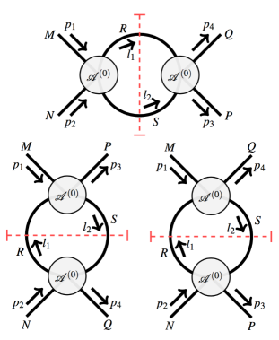
Figure 2: Diagrams representing s-, t- and u-channel cuts contributing to the four-point one-loop amplitude.

Notice that tadpole graphs, having no physical two-particle cuts, are by definition ignored in this procedure. To proceed, in each case one uses the momentum conservation at the vertex involving the momentum $p_{1}$ to integrate over $l_{2}$, e.g. for the $s$-channel

$$\!\!\!\!\!\!\!\!\!\!\!\!\!\!\!\!\!\!\!\!\!\!\!\mathcal{\widetilde{A}}^{(1)}{}^{PQ}_{MN}(p_{1},p_{2},p_{3},p_{4})|_{s-cut}=\int\frac{d^{2}l_{1}}{(2\pi)^{2}}\,i\pi\delta^{+}({l_{1}}^{2}-1)\,i\pi\delta^{+}(({l_{1}}-{p_{1}}-{p_{2}})^{2}-1)$$

$$\qquad\times\,\,\widetilde{\mathcal{A}}^{(0)}{}_{MN}^{RS}({p_{1},p_{2},l_{1},-l_{1}+p_{1}+p_{2}})\,\widetilde{\mathcal{A}}^{(0)}{}_{SR}^{PQ}({-l_{1}+p_{1}+p_{2},l_{1},p_{3},p_{4}})\,.$$

The simplicity of the two-dimensional kinematics and of being at one loop plays now its role, since in each of the integrals the set of zeroes of the $\delta$-functions is a discrete set, and the cut loop-momenta are frozen to specific values . This allows us to pull out the tree-level amplitudes with the loop-momenta evaluated at those zeroes . In what remains, following standard unitarity computations [64], we apply the replacement $i\pi\delta^{+}(l^{2}-1)\longrightarrow\tfrac{1}{l^{2}-1}$ (i.e. the Cutkowsky rule in reverse order) which sets loop momenta back off-shell, thus reconstructing scalar bubbles. This allows to rebuild, from its imaginary part, the cut-constructible piece of the amplitude and of the S-matrix, via [62]

$$S_{MN}^{PQ}(p_{1},p_{2})\equiv\frac{J(p_{1},p_{2})}{4\epsilon_{1}\epsilon_{2}}\widetilde{\mathcal{A}}_{MN}^{PQ}(p_{1},p_{2},p_{1},p_{2})~{}.$$ (2.19)

where the Jacobian $J(p_{1},p_{2})=1/(\partial\epsilon_{{\rm p}_{1}}/\partial{\rm p}_{1}-\partial\epsilon_{{\rm p}_{2}}/\partial{\rm p}_{2})$ depends on the dispersion relation $\epsilon_{\rm p}$, on-shell energy associated to ${\rm p}$ (the spatial momentum) for the theory at hand. The expression for the one-loop S-matrix elements is given by the following simple sum of products of two tree-level amplitudes 

$${S^{(1)}}{}_{MN}^{PQ}(p_{1},p_{2})=\frac{1}{4(\epsilon_{2}\,{\rm p}_{1}-\epsilon_{1}\,{\rm p}_{2})}\,\Big{[}{\tilde{S}^{(0)}}{}_{MN}^{RS}(p_{1},p_{2}){\tilde{S}^{(0)}}{}_{RS}^{PQ}(p_{1},p_{2})\,I_{p_{1}+p_{2}}$$ (2.20)

$$+{\tilde{S}^{(0)}}{}_{MR}^{SP}(p_{1},p_{1}){\tilde{S}^{(0)}}{}_{SN}^{RQ}(p_{1},p_{2})\,I_{0}\vphantom{\frac{1}{4(\epsilon_{2}\,{\rm p}_{1}-\epsilon_{1}\,{\rm p}_{2})}}+{\tilde{S}^{(0)}}{}_{MR}^{SQ}(p_{1},p_{2}){\tilde{S}^{(0)}}{}_{SN}^{PR}(p_{1},p_{2})\,I_{p_{1}-p_{2}}\,\Big{]}$$

where the coefficients are given in terms of the bubble integral

$$I_{p}=\int\frac{d^{2}q}{(2\pi)^{2}}\frac{1}{(q^{2}-1+i\epsilon)((q-p)^{2}-1+i\epsilon)}~{}$$ (2.21)

and read explicitly 

$$I_{p_{1}+p_{2}}=\frac{i\pi-\operatorname{arsinh}(\epsilon_{2}\,{\rm p}_{1}-\epsilon_{1}\,{\rm p}_{2})}{4\pi i\,(\epsilon_{2}\,{\rm p}_{1}-\epsilon_{1}\,{\rm p}_{2})},~{}~{}I_{0}=\frac{1}{4\pi i},~{}~{}I_{p_{1}-p_{2}}=\frac{\operatorname{arsinh}(\epsilon_{2}\,{\rm p}_{1}-\epsilon_{1}\,{\rm p}_{2})}{4\pi i\,(\epsilon_{2}\,{\rm p}_{1}-\epsilon_{1}\,{\rm p}_{2})}~{}.$$

As it only involves the scalar bubble integral in two dimensions, the result (2.20) following from our procedure is inherently finite. No additional regularization is required and the result can be compared directly with the $2\to 2$ particle S-matrix (following from the finite or renormalized four-point amplitude) found using standard perturbation theory. Of course, this need not be the case for the original bubble integrals before cutting – due to factors of loop-momentum in the numerators. These divergences, along with those coming from tadpole graphs, which are not considered in this procedure, should be taken into account for the renormalization of the theory. We have not investigated this issue, since all the theories considered in [62]  are either UV-finite or renormalizable. The method, applied to various models, has shown enough evidence to postulate that supersymmetric, integrable two-dimensional theories should be cut-constructible via standard unitarity methods. For bosonic theories with integrability, agreement was found with perturbation theory up to a finite shift in the coupling. In the case of the superstring worldsheet models in $AdS_{5}\times S^{5}$ [62] and $AdS_{3}\times S^{3}\times M^{4}$ [65], the method allowed non-trivial confirmations of the integrability prediction together with conjectures (then confirmed) on the one-loop phases.

3 $AdS_{5}\times S^{5}$ superstring on a lattice

The natural, genuinely field-theoretical way to investigate the finite-coupling region and in general the non-perturbative realm of a quantum field theory is to discretize the spacetime where the model lives, and proceed with numerical methods for the lattice field theory so defined. A rich and interesting program of putting $\mathcal{N}=4$ SYM a space-time lattice is being carried out for some years [66, 67, 68, 69, 70] . Alternatively, one could discretize the worldsheet spanned by the Green-Schwarz string embedded in $AdS_{5}\times S^{5}$. If the aim is a test of the AdS/CFT correspondence and/or the integrability of the string sigma model, it is is obviously computationally cheaper to use a two-dimensional grid, rather than a four-dimensional one, where no gauge degrees of freedom are present and all fields are assigned to sites - so that only scalar fields (some of which anticommuting) appear in the relevant action. Also, although we are dealing with superstrings, there is here no subtlety involved with putting supersymmetry on the lattice (see e.g. [13]), both because of the Green-Schwarz formulation of the action (with supersymmetry only manifest in the target space) and because $\kappa$-symmetry is gauge-fixed. In general, one merit of this analysis is to explore another route via which lattice simulations  could become a potentially efficient tool in numerical holography. Following the earlier proposal of [10], such a route has been taken in [11, 12] to investigate relevant observables in AdS/CFT, discretizing the dual two-dimensional string worldsheet. There, the focus is on particularly important observables completely “solved” via integrability [79]: the cusp anomalous dimension of $\mathcal{N}=4$ SYM – measured by the path integral of an open string bounded by a null-cusped Wilson loop at the AdS boundary – and the spectrum of excitations around the corresponding string minimal surface. The relevant string worldsheet theory, an AdS-lightcone gauge-fixed action [80, 54], is a highly non-trivial 2d non-linear sigma-model with rich non-perturbative dynamics. On the lattice, several subtleties appear (fermion doublers, complex phases) which require special treatment, as we sketch below.

3.1 The observable in the continuum

The cusp anomaly of $\mathcal{N}=4$ SYM governs the renormalization of a cusped Wilson loop, and according to AdS/CFT should be represented by the path integral of an open string ending on the loop at the AdS boundary

$$\begin{split}\langle W[C_{\rm cusp}]\rangle\equiv Z_{\rm cusp}&=\int[D\delta X][D\delta\Psi]\,e^{-S_{\rm cusp}[X_{\rm cl}+\delta X,\delta\Psi]}\\ &=e^{-\Gamma_{\rm eff}}\equiv e^{-\frac{1}{8}f(g)\,V_{2}}~{}.\end{split}$$ (4.1)

Above, $X_{\rm cl}=X_{\rm cl}(t,s)$ - with $t,s$ the temporal and spatial coordinate spanning the string worldsheet - is the relevant classical solution [55], $S_{\rm cusp}[X+\delta X,\delta\Psi]$ is the action for field fluctuations over it – the fields being both bosonic and fermionic string coordinates $X(t,s),~{}\Psi(t,s)$ – and is reported below in equation (4.3) in terms of the effective bosonic and fermionic degrees of freedom remaining after gauge-fixing. Being an homogenous solution, the worldsheet volume simply factorizes out  in front of the function of the coupling $f(g)$, as in the last equivalence above. Rather than partition functions, in a lattice approach it is natural to study vacuum expectation values. In simulating the vacuum expectation value of the “cusp” action

$$\langle S_{\rm cusp}\rangle = \frac{\int[D\delta X][D\delta\Psi]\,S_{\rm cusp}\,e^{-S_{\rm cusp}}}{\int[D\delta X][D\delta\Psi]\,e^{-S_{\rm cusp}}}=-g\,\frac{d\ln Z_{\rm cusp}}{dg}\equiv g\,\frac{V_{2}}{8}\,f^{\prime}(g)~{},$$ (4.2)

one therefore obtains information on the derivative of the scaling function. In the continuum, the $AdS_{5}\times S^{5}$ superstring action $S_{\rm cusp}$ describing quantum fluctuations around the null-cusp background is [55] (after Wick-rotation)

$$\!\!\!\!\!\!\!\!\!\!\!\!S_{\rm cusp}=g\int dtds~{}\textstyle\Big{\{}|\partial_{t}x+\textstyle{\frac{1}{2}}x|^{2}+\frac{1}{{z}^{4}}|\partial_{s}{x}-\textstyle{\frac{1}{2}}{x}|^{2}-\textstyle{\frac{1}{{z}^{2}}}\left({\eta}^{i}{\eta}_{i}\right)^{2}+\frac{1}{{z}^{4}}\left(\partial_{s}{z}^{M}-\textstyle{\frac{1}{2}}{z}^{M}\right)^{2}$$

$$\!\!\!\!\!\!\!\!\!\!\!\!\textstyle+\textstyle{\big{(}\partial_{t}z^{M}+\frac{1}{2}{z}^{M}+\frac{i}{{z}^{2}}{z}_{N}{\eta}_{i}\left(\rho^{MN}\right)_{\phantom{i}j}^{i}{\eta}^{j}\big{)}^{2}}+i\left({\theta}^{i}\partial_{t}{\theta}_{i}+{\eta}^{i}\partial_{t}{\eta}_{i}+{\theta}_{i}\partial_{t}{\theta}^{i}+{\eta}_{i}\partial_{t}{\eta}^{i}\right)$$

$$\!\!\!\!\!\!\!\!\!\!\!\!\textstyle+2i\Big{[}\textstyle{\frac{1}{z^{3}}}z^{M}{\eta}^{i}\left(\rho^{M}\right)_{ij}\left(\partial_{s}\theta^{j}-\textstyle{\frac{1}{2}}\theta^{j}-\frac{i}{{z}}{\eta}^{j}\left(\partial_{s}{x}-\frac{1}{2}{x}\right)\right)$$

$$\textstyle{+\frac{1}{{z}^{3}}{z}^{M}{\eta}_{i}(\rho_{M}^{\dagger})^{ij}\left(\partial_{s}{\theta}_{j}-\frac{1}{2}{\theta}_{j}+\frac{i}{{z}}{\eta}_{j}\left(\partial_{s}{x}-\frac{1}{2}{x}\right)^{*}\right)\Big{]}\,\Big{\}}}$$ (4.3)

Above, $x,x^{*}$ are the two bosonic $AdS_{5}$ (coordinate) fields transverse to the $AdS_{3}$ subspace of the classical solution, and $z^{M}\,(M=1,\cdots,6)$ are the bosonic coordinates of the $AdS_{5}\times S^{5}$ background in Poincaré parametrization, with $z=\sqrt{z_{M}z^{M}}$, remaining after fixing the AdS light-cone gauge. The fields $\theta_{i},\eta_{i},\,i=1,2,3,4$ are 4+4 complex anticommuting variables for which $\theta^{i}=(\theta_{i})^{\dagger},$ $\eta^{i}=(\eta_{i})^{\dagger}$. They transform in the fundamental representation of the $SU(4)$ R-symmetry and do not carry (Lorentz) spinor indices. The matrices $\rho^{M}_{ij}$ are the off-diagonal blocks of $SO(6)$ Dirac matrices $\gamma^{M}$ in the chiral representation and $(\rho^{MN})_{i}^{\hphantom{i}j}=(\rho^{[M}\rho^{\dagger N]})_{i}^{\hphantom{i}j}$ are the $SO(6)$ generators. In (4.3) – where a massive parameter $m\sim P^{+}$, usually set to one, is restored – local bosonic (diffeomorphism) and fermionic ($\kappa$-) symmetries originally present have been fixed. With this action one can directly proceed to the perturbative evaluation of the cusp anomaly ($K$ is the Catalan constant) and of the dispersion relation for the field excitations

$$\begin{split}f(g)&=4\,g\,\Big{(}1-\frac{3\log 2}{4\pi\,g}-\frac{K}{16\,\pi^{2}\,g^{2}}+\mathcal{O}(g^{-3})\Big{)}\\ m^{2}_{x}(g)&=\frac{m^{2}}{2}\,\Big{(}1-\frac{1}{8\,g}+\mathcal{O}(g^{-2})\Big{)}~{}.\end{split}$$ (4.4)

While the bosonic part of (4.3) can be easily discretized and simulated, Graßmann-odd fields are formally integrated out, letting their determinant to become part – via exponentiation in terms of pseudo-fermions, see (4.9) below – of the Boltzmann weight of each configuration in the statistical ensemble. In the case of higher-order fermionic interactions – as in (4.3), where they are at most quartic – this is possible via the introduction of auxiliary fields realizing a linearization. The most natural linearization [10] introduces $7$ real auxiliary fields, one scalar $\phi$ and a $SO(6)$ vector field $\phi_{M}$, with a Hubbard-Stratonovich transformation

$$\!\!\!\!\!\!\!e^{-g\int dtds\Big{[}-\textstyle{\frac{1}{{z}^{2}}}\left({\eta}^{i}{\eta}_{i}\right)^{2}+\Big{(}\textstyle{\frac{i}{{z}^{2}}}{z}_{N}{\eta}_{i}{\rho^{MN}}_{\phantom{i}j}^{i}{\eta}^{j}\Big{)}^{2}\Big{]}}$$ (4.5)

$$\!\!\!\!\!\!\!\sim\!\int\!\!D\phi D\phi^{M}\,e^{-g\int dtds\,[\textstyle\frac{1}{2}{\phi}^{2}+\frac{\sqrt{2}}{z}\phi\,\eta^{2}+\frac{1}{2}({\phi}_{M})^{2}-i\,\frac{\sqrt{2}}{z^{2}}\phi^{M}{z}_{N}\,\big{(}i\,{\eta}_{i}{\rho^{MN}}_{\phantom{i}j}^{i}{\eta}^{j}\big{)}]}~{}.$$

Above, in the second line we have written the Lagrangian for $\phi^{M}$ so to emphasize that it has an imaginary part, due to the fact that the bilinear form in round brackets is hermitian

$$\!\!\!\!\!\!\Big{(}i\,\eta_{i}{\rho^{MN}}^{i}{}_{j}\eta^{j}\Big{)}^{\dagger}=-i(\eta^{j})^{\dagger}({\rho^{MN}}^{i}{}_{j})^{*}(\eta_{i})^{\dagger}=-i\eta_{j}\,{\rho^{MN}}_{i}{}^{j}\,\eta^{i}=i\eta_{j}\,{\rho^{MN}}^{j}{}_{i}\,\eta^{i}\,,$$ (4.6)

as follows from the properties of the $SO(6)$ generators. Since the auxiliary vector field $\phi^{M}$ has real support, the Yukawa-term for it sets a priori a phase problem, the only question being whether the latter is treatable via standard reweighing. After the transformation (4.5), the corresponding Lagrangian reads

$$\!\!\!\!\!\!\!\!\!\!\!\!\!\!\!{\cal L} = \!\textstyle{|\partial_{t}{x}+\!\frac{m}{2}{x}|}^{2}+\!\frac{1}{{z}^{4}}{|\partial_{s}{x}-\!\frac{m}{2}{x}|}^{2}+\!(\partial_{t}{z}^{M}+\!\frac{1}{2}{z}^{M})^{2}+\!\frac{1}{{z}^{4}}(\partial_{s}{z}^{M}-\!\frac{m}{2}{z}^{M})^{2}$$ (4.7)

$$+\!\frac{1}{2}{\phi}^{2}+\!\frac{1}{2}({\phi}_{M})^{2}+\!\psi^{T}O_{F}\psi\,$$

with $\psi\equiv({\theta}^{i},{\theta}_{i},{\eta}^{i},{\eta}_{i})$ and

$$\!\!\!\!\!\!\!\!\!\!\!\!\!\!\!\!\!\!\!\!\!\textstyle{O_{F}=\left(\!\!\!\!\begin{array}[]{cccc}\!\!\!\!0&\!\!\!\!i\partial_{t}&\!\!\!\!\textstyle{-\mathrm{i}\rho^{M}\left(\partial_{s}+\frac{m}{2}\right)\frac{{z}^{M}}{{z}^{3}}}&\!\!\!\!0\\ \mathrm{i}\partial_{t}&0&0&-\mathrm{i}\rho_{M}^{\dagger}\left(\partial_{s}+\frac{m}{2}\right)\frac{{z}^{M}}{{z}^{3}}\\ \mathrm{i}\frac{{z}^{M}}{{z}^{3}}\rho^{M}\left(\partial_{s}-\frac{m}{2}\right)&0&2\frac{{z}^{M}}{{z}^{4}}\rho^{M}\left(\partial_{s}{x}-m\frac{{x}}{2}\right)&i\partial_{t}-A^{T}\\ 0&\mathrm{i}\frac{{z}^{M}}{{z}^{3}}\rho_{M}^{\dagger}\left(\partial_{s}-\frac{m}{2}\right)&\mathrm{i}\partial_{t}+A&-2\frac{{z}^{M}}{{z}^{4}}\rho_{M}^{\dagger}\left(\partial_{s}{x}^{*}-m\frac{{x}}{2}^{*}\right)\end{array}\!\!\!\!\right),}$$

$$A=\frac{1}{\sqrt{2}{z}^{2}}{\phi}_{M}\rho^{MN}{z}_{N}-\frac{1}{\sqrt{2}{z}}{\phi}\,+\mathrm{i}\,\frac{{z}_{N}}{{z}^{2}}\rho^{MN}\,\partial_{t}{z}^{M}~{}.$$ (4.8)

The quadratic fermionic contribution resulting from linearization gives then formally a Pfaffian ${\rm Pf}\,O_{F}$, which - in order to enter the Boltzmann weight and thus be interpreted as a probability - should be positive definite. For this reason, one proceeds as follows

$$\!\!\!\!\int\!\!D\Psi~{}e^{-\textstyle\int dtds\,\Psi^{T}O_{F}\Psi}={\rm Pf}\,O_{F}\equiv(\det O_{F}\,O^{\dagger}_{F})^{\frac{1}{4}}=\int\!\!D\xi D\bar{\xi}\,e^{-\int dtds\,\bar{\xi}(O_{F}O^{\dagger}_{F})^{-\frac{1}{4}}\,\xi}~{},$$ (4.9)

where the second equivalence obviously ignores potential phases or anomalies. The values of the discretised (scalar) fields are assigned to each lattice site, with periodic boundary conditions for all the fields except for antiperiodic temporal boundary conditions in the case of fermions. The discrete approximation of continuum derivatives are finite difference operators defined on the lattice. A Wilson-like lattice operator must be introduced, such that fermion doublers are suppressed and the one-loop constant $-3\ln 2/\pi$ in (4.4) is recovered in lattice perturbation theory.

3.2 Simulations

The Monte Carlo evolution of the action (4.7) is generated by the standard Rational Hybrid Monte Carlo (RHMC) algorithm, with a rational approximation (Remez algorithm) for the inverse fractional power in the last equation of (4.9), as in [10]. In the continuum model there are two parameters, the dimensionless coupling $g=\frac{\sqrt{\lambda}}{4\pi}$ and the mass scale $m$. In taking the continuum limit, the dimensionless physical quantities that it is natural to keep constant are the physical masses of the field excitations rescaled by $L$, the spatial lattice extent. This is our line of constant physics. For the example in (4.4), this means

$$L^{2}\,m^{2}_{x}=\text{const}\,,\qquad~{}~{}\text{which leads to}\qquad~{}~{}L^{2}\,m^{2}\equiv(NM)^{2}=\text{const}\,,$$ (4.10)

where we defined the dimensionless $M=ma$ with the lattice spacing $a$. The second equation in (4.10) relies first on the assumption that $g$ is not renormalized, which is suggested by lattice perturbation theory. Second, one should investigate whether the second relation in (4.4), and the analogue ones for the other fields of the model, are still true in the discretized model - i.e. the physical masses undergo only a finite renormalization. In this case, at each fixed $g$ fixing $L^{2}~{}m^{2}$ constant would be enough to keep the rescaled physical masses constant, namely no tuning of the “bare” parameter $m$ would be necessary. In [12], we considered the example of bosonic $x,x^{*}$ correlators, whose asymptotic exponential decay is governed by the physical mass ${m_{x}}_{\rm LAT}$, as from the partially Fourier transformed

$$\!\!\!\!\!\!\!C_{x}(t;\,0)~{}\stackrel{{\scriptstyle t\gg 1}}{{\sim}}~{}e^{-t\,{m_{x}}_{\rm LAT}},\qquad{m_{x}}_{\rm LAT}=\lim_{T,\,t\to\infty}m^{\textrm{eff}}_{x}\equiv\lim_{T,\,t\to\infty,}\frac{1}{a}\log\frac{C_{x}(t;\,0)}{C_{x}(t+a;\,0)}.$$ (4.11)

On the lattice ${m_{x}}_{\rm LAT}$ is usefully obtained as a limit of an effective mass, the discretized logarithmich derivative above, that in Fig. 3 is measured as a function of the time t (in units of ${m_{x}}_{\rm LAT}$) for different lattice sizes. No ($1/a$) divergence is found, and in the large $g$ region that we investigate the ratio considered approaches the expected continuum value $1/2$. Having this as hint corroborating the choice of the line of constant physics, and because with the proposed discretization we recover in perturbation theory the one-loop cusp anomaly, we assume that in the discretized model no further scale but the lattice spacing $a$ is present. Any observable $F_{\rm LAT}$ is therefore a function $F_{\rm LAT}=F_{\rm LAT}(g,N,M)$ of the input (dimensionless) parameters $g=\frac{\sqrt{\lambda}}{4\pi}$, $N=\frac{L}{a}$ and $M=a\,m$. At fixed coupling $g$ and fixed $m\,L\equiv M\,N$ (large enough so to keep finite volume effects $\sim e^{-m\,L}$ small), $F_{\rm LAT}$ is evaluated for different values of $N$. The continuum limit – which we do not attempt here – is then obtained extrapolating to infinite $N$.

In measuring the action (4.2) on the lattice, we are supposed to recover the following general behavior

$$\frac{\langle S_{\rm LAT}\rangle}{N^{2}}=\frac{c}{2}+\frac{1}{8}\,M^{2}\,g\,f^{\prime}(g)\,,$$ (4.12)

where we have reinserted the parameter $m$, used that $V_{2}=a^{2}\,N^{2}$ and added a constant contribution in $g$ which takes into account possible coupling-dependent Jacobians relating the (derivative of the) partition function on the lattice to the one in the continuum. Measurements for the ratio $\frac{\langle S_{LAT}\rangle-c\,N^{2}/2}{M^{2}\,N^{2}\,g/2}=\frac{f^{\prime}(g)}{4}~{}$ are, at large $g$, in good agreement with $\frac{c}{2}=7.5(1)$, consistently with the with the counting of those degrees of freedom which appear quadratically, and multiplying $g$, in the action – the number of bosons . Having determined with good precision the coefficient of the divergence, one proceeds first fixing it to be exactly $c=15$ and subtracting it from the action. At large $g$, a good agreement is found with the leading order prediction in (4.4) for which $f^{\prime}(g)=4$. For lower values of $g$ one observes deviations that obstruct the continuum limit and signal the presence of further quadratic ($\sim N^{2}$) divergences. It seems natural to relate these power-divergences to those arising in continuum perturbation theory and mentioned in the previous Section, where they are usually set to zero using dimensional regularization. From the perspective of a hard cut-off regularization like the lattice one, this is related to the emergence in the continuum limit of power divergences – quadratic, in the present two-dimensional case – induced by mixing of the (scalar) Lagrangian with the identity operator under UV renormalization. One may proceed with a non-perturbative subtraction of these divergences. A simple look at Fig. 4 shows that, in the perturbative region, our analysis – and the related assumption for the finite rescaling of the coupling – is in good qualitative agreement with the integrability prediction. About direct comparison with the perturbative series, the plot in Fig. 4 does not catch the minimal upward trend of the first correction to the expected large g behavior $f^{\prime}(g)/4\sim 1$ - we are considering the derivative of eq. (21) and the first correction is (positive and) too small, about 2 percent, if compared to the statistical error. Notice that, again under the assumption that such simple relation between the couplings exists – something that within our error bars cannot be excluded – the nonperturbative regime beginning with $g_{c}=1$ would start at $g=25$, implying that our simulations at $g=10,5$ would already test a fully non-perturbative regime of the string sigma-model under investigation. In proximity to $g\sim 1$, severe fluctuations appear in the averaged complex phase of the Pfaffian – see Figure 5 – signaling the sign problem mentioned above. Interestingly, at least some steps in the direction of solving this problem can be done analytically [81, 82]. A new auxiliary field representation of the four-fermi term may be realized, following an algebraic manipulation from which an hermitian Lagrangian linearized in fermions results, leads to a Pfaffian of the quadratic fermionic operator $O_{F}$ which is real, $({\rm Pf}\,O_{F})^{2}=\det O_{F}\geq 0$. Although a sign ambiguity remains, as the Pfaffian is still not positive definite, ${\rm Pf}\,O_{F}=\pm\det O_{F}$, this is an important advancement in the efficiency of the simulations, as it allows eliminating systematic errors and identifying with precision the region of parameter space where information on nonperturbative physics may be captured.

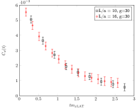
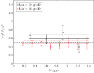
Figure 3: Correlator $C_{x}(t)=\sum_{s_{1},s_{2}}\langle x(t,s_{1})x^{*}(0,s_{2})\rangle$ of bosonic fields $x,x^{*}$ (left panel) and corresponding effective mass $m^{\rm eff}_{x}=\frac{1}{a}\ln\frac{C_{x}(t)}{C_{x}(t+a)}$ normalized by $m^{2}$ (right panel), plotted as functions of the time $t$ in units of ${m_{x}}_{\rm LAT}$ for different $g$ and lattice sizes. The flatness of the effective mass indicates that the ground state saturates the correlation function, and allows for a reliable extraction of the mass of the $x$-excitation. Data points are masked by large errorbars for time scales greater than unity because the signal of the correlator degrades exponentially compared with the statistical noise.

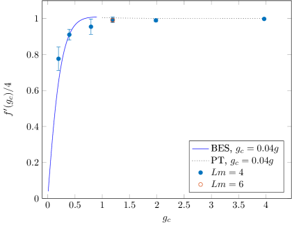
Figure 4: Plot for $f^{\prime}(g)/4$ as a function of the (bare) continuum coupling $g_{c}$ under the hypothesis that the latter is just a finite rescaling of the lattice bare coupling $g$ ($g_{c}=0.04\,g$). The dashed line represents the first few terms in the perturbative series, the continuous line is obtained from a numerical solution of the BES equation and represents therefore the prediction from the integrability of the model. The simulations at $g=30$, $m\,L=6$ (orange point) are used for a check of the finite volume effects, that appear to be within statistical errors.

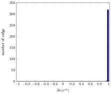
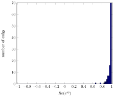
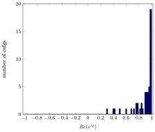
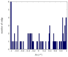
Figure 5: Histograms for the frequency of the real part of the reweighting phase factor $e^{i\theta}$ of the Pfaffian ${\rm Pf}\,O_{F}=|(\det O_{F})^{\frac{1}{2}}|\,e^{i\theta}$, based on the ensembles generated at $g=30,10,5,1$ (from left to right, top to down) for $L/a=8$.

4 Discussion and outlook

We have reviewed and discussed perturbative and non-perturbative approaches to the quantization of the Green-Schwarz string in AdS backgrounds with RR-fluxes, with an emphasis on the use of direct quantum field theory methods and on the cross-fertilization of theoretical tools well-established in gauge field theories to the string worldsheet context.

In dealing with sigma-model perturbation theory, crucial subtleties appear in evaluating regularised functional determinants for string fluctuations and the computational technology for them has to be carefully adjusted to the problem at hand. It would be important to develop a diffeomorphism-preserving regularization scheme which retains the efficiency of the Gelf’and-Yaglom method for one-dimensional cases, and extend such techniques to regularised super-traces and super-determinants so to address a uniform way of treating BPS and non-BPS observables . It would be extremely interesting to elucidate the role of the measure (structure and normalization) in the string path integral for supersymmetric configurations.

Going beyond perturbation theory, a new research line has been addressed, which employs Montecarlo simulations to investigate observables defined on suitably discretized euclidean string worldsheets. At a fundamental level, this is the natural setup for verifying with unequaled definiteness the holographic conjecture and the exact methods that “solve” various sectors of the AdS/CFT system. Lattice methods are also the most suitable candidates for the study of several observables and backgrounds for which alternative techniques to go beyond perturbation theory are not existing (string backgrounds which are not classically integrable) or yet at a preliminary stage (correlators of string vertex operators and dual gauge theory correlation functions).

It is important to emphasize that the analysis here carried out is far from being a non-perturbative definition, à la Wilson lattice-QCD, of the Green-Schwarz worldsheet string model. For this purpose one should work with a Lagrangian which is invariant under the local symmetries - bosonic diffeomorphisms and $\kappa$-symmetry - of the model, while as mentioned we make use of an action which fixes them all. There is however a number of reasons which make this model interesting for lattice investigations, within and hopefully beyond the community interested in holographic models.

As computational playground this is an interesting one on its own, allowing in principle for explicit investigations/improvements of algorithms: a highly-nontrivial two-dimensional model with four-fermion interactions, for which relevant observables have not only, through AdS/CFT, an explicit analytic strong coupling expansion – the perturbative series in the dual gauge theory – but also, through AdS/CFT and the assumption of integrability, an explicit numerical prediction at all couplings.

The results discussed here open the way to a variety of further explorations and developements. A natural evolution consists in treating strings propagating in those backgrounds (the ten-dimensional $AdS_{4}\times CP^{3}$, $AdS^{3}\times S^{3}\times T^{4}$, $AdS_{3}\times S^{3}\times S^{3}\times S^{1}$ supported by RR fluxes) relevant for lower-dimensional formulations of the correspondence, for which several predictions exist from integrability, and for which an independent their AdS-light-cone gauge-fixed Lagrangians are expected to be considerably more involved than in the prototypical case, but still with vertices at most quartic in fermions. In all the novel cases of study the presence of massless fermionic modes is expected to require an ad-hoc treatment, one possibility being to work in a finite-volume setting like the Schrödinger functional scheme. It would be crucial a thorough study of the possible sign problem - related to the absence of positive definiteness of the fermion Pfaffian - that is likely to appear at large values of the string tension as in the prototypical case. This may consists in carving out the region of parameter space where the sign ambiguity is not severe and clarifying whether non-perturbative physics is obtainable. One may then verify the possibility of track down this ambiguity to the behaviour of a smaller set of degrees of freedom – such analysis may profit, at least pedagogically, from recent progress on the analysis of the sign problem in (considerably simpler) models with quartic fermionic interactions [83, 84]. Also, it would be very interesting to explore the discretization of the gauge-fixed string action of [85], whose relevance from the point of view of the string/gauge gravity correspondence is far less clear, but that being only quadratic in fermions may lead to considerable simplifications in the general analysis.

References

- [1] N. Beisert et al., “Review of AdS/CFT Integrability: An Overview”, Lett. Math. Phys. 99, 3 (2012), arXiv:1012.3982.
- [2] V. Pestun, “Localization of gauge theory on a four-sphere and supersymmetric Wilson loops”, Commun.Math.Phys. 313, 71 (2012), arXiv:0712.2824.
- [3] V. Pestun et al., “Localization techniques in quantum field theories”, arXiv:1608.02952.
- [4] D. Correa, J. Henn, J. Maldacena and A. Sever, “An exact formula for the radiation of a moving quark in super Yang Mills”, JHEP 1206, 048 (2012), arXiv:1202.4455.
- [5] S. S. Gubser, I. R. Klebanov and A. M. Polyakov, “A semi-classical limit of the gauge/string correspondence”, Nucl. Phys. B636, 99 (2002), hep-th/0204051.
- [6] S. Frolov and A. A. Tseytlin, “Semiclassical quantization of rotating superstring in ”, JHEP 0206, 007 (2002), hep-th/0204226.
- [7] T. McLoughlin, “Review of AdS/CFT Integrability, Chapter II.2: Quantum Strings in ”, Lett. Math. Phys. 99, 127 (2012), arXiv:1012.3987.
- [8] A. M. Polyakov, “Conformal fixed points of unidentified gauge theories”, Mod. Phys. Lett. A19, 1649 (2004), hep-th/0405106, [,1159(2004)].
- [9] R. Roiban and A. A. Tseytlin, “Strong-coupling expansion of cusp anomaly from quantum superstring”, JHEP 0711, 016 (2007), arXiv:0709.0681.
- [10] R. W. McKeown and R. Roiban, “The quantum superstring at finite coupling”, arXiv:1308.4875.
- [11] V. Forini, L. Bianchi, M. S. Bianchi, B. Leder and E. Vescovi, “Lattice and string worldsheet in AdS/CFT: a numerical study”, PoS LATTICE2015, 244 (2015), arXiv:1601.04670, in: “Proceedings, 33rd International Symposium on Lattice Field Theory (Lattice 2015)”, 244p.
- [12] L. Bianchi, M. S. Bianchi, V. Forini, B. Leder and E. Vescovi, “Green-Schwarz superstring on the lattice”, JHEP 1607, 014 (2016), arXiv:1605.01726.
- [13] S. Catterall, J. Giedt, D. Schaich, P. H. Damgaard and T. DeGrand, “Results from lattice simulations of supersymmetric Yang-Mills”, PoS LATTICE2014, 267 (2014), arXiv:1411.0166, in: “Proceedings, 32nd International Symposium on Lattice Field Theory (Lattice 2014)”, 267p.
- [14] C. G. Callan, Jr. and L. Thorlacius, “Sigma models and string theory”, in: “In *Providence 1988, Proceedings, Particles, strings and supernovae, vol. 2* 795-878.”.
- [15] N. Drukker, D. J. Gross and A. A. Tseytlin, “Green-Schwarz string in AdS5xS5: Semiclassical partition function”, JHEP 0004, 021 (2000), hep-th/0001204.
- [16] S. Frolov and A. A. Tseytlin, “Multispin string solutions in ”, Nucl.Phys. B668, 77 (2003), hep-th/0304255.
- [17] S. Frolov and A. A. Tseytlin, “Quantizing three spin string solution in ”, JHEP 0307, 016 (2003), hep-th/0306130.
- [18] S. Frolov, I. Park and A. A. Tseytlin, “On one-loop correction to energy of spinning strings in ”, Phys.Rev. D71, 026006 (2005), hep-th/0408187.
- [19] I. Park, A. Tirziu and A. A. Tseytlin, “Spinning strings in : One-loop correction to energy in SL(2) sector”, JHEP 0503, 013 (2005), hep-th/0501203.
- [20] N. Beisert, A. A. Tseytlin and K. Zarembo, “Matching quantum strings to quantum spins: One-loop versus finite-size corrections”, Nucl.Phys. B715, 190 (2005), hep-th/0502173.
- [21] I. M. Gelfand and A. M. Yaglom, “Integration in functional spaces and it applications in quantum physics”, J. Math. Phys. 1, 48 (1960).
- [22] R. Forman, “Functional determinants and geometry”, Invent. math. 88, 447 (1987).
- [23] R. Forman, “Functional determinants and geometry (Erratum)”, Invent. math. 108, 453 (1992).
- [24] A. J. McKane and M. B. Tarlie, “Regularization of functional determinants using boundary perturbations”, J.Phys. A28, 6931 (1995), cond-mat/9509126.
- [25] K. Kirsten and A. J. McKane, “Functional determinants by contour integration methods”, Annals Phys. 308, 502 (2003), math-ph/0305010.
- [26] K. Kirsten and A. J. McKane, “Functional determinants for general Sturm-Liouville problems”, J.Phys. A37, 4649 (2004), math-ph/0403050.
- [27] K. Kirsten and P. Loya, “Computation of determinants using contour integrals”, Am. J. Phys. 76, 60 (2008), arXiv:0707.3755.
- [28] G. V. Dunne, “Functional determinants in quantum field theory”, J. Phys. A41, 304006 (2008), arXiv:0711.1178, in: “Proceedings, 5th International Symposium on Quantum theory and symmetries (QTS5)”, 304006p.
- [29] V. Forini, V. Giangreco M. Puletti, L. Griguolo, D. Seminara and E. Vescovi, “Precision calculation of 1/4-BPS Wilson loops in ”, JHEP 1602, 105 (2016), arXiv:1512.00841.
- [30] M. Beccaria, G. V. Dunne, V. Forini, M. Pawellek and A. A. Tseytlin, “Exact computation of one-loop correction to energy of spinning folded string in AdS5xS5”, J.Phys. A43, 165402 (2010), arXiv:1001.4018.
- [31] V. Forini, V. G. M. Puletti, M. Pawellek and E. Vescovi, “One-loop spectroscopy of semiclassically quantized strings: bosonic sector”, J.Phys. A48, 085401 (2015), arXiv:1409.8674.
- [32] M. Kruczenski, “Spin chains and string theory”, Phys. Rev. Lett. 93, 161602 (2004), hep-th/0311203.
- [33] E. S. Fradkin and A. A. Tseytlin, “ON QUANTIZED STRING MODELS”, Annals Phys. 143, 413 (1982).
- [34] M. Kruczenski and A. Tirziu, “Matching the circular Wilson loop with dual open string solution at 1-loop in strong coupling”, JHEP 0805, 064 (2008), arXiv:0803.0315.
- [35] E. I. Buchbinder and A. A. Tseytlin, “ correction in the D3-brane description of a circular Wilson loop at strong coupling”, Phys. Rev. D89, 126008 (2014), arXiv:1404.4952.
- [36] N. Drukker and B. Fiol, “On the integrability of Wilson loops in AdS5xS5: Some periodic ansatze”, JHEP 0601, 056 (2006), hep-th/0506058.
- [37] N. Drukker, “1/4 BPS circular loops, unstable world-sheet instantons and the matrix model”, JHEP 0609, 004 (2006), hep-th/0605151.
- [38] N. Drukker, S. Giombi, R. Ricci and D. Trancanelli, “Supersymmetric Wilson loops on ”, JHEP 0805, 017 (2008), arXiv:0711.3226.
- [39] V. Forini, V. G. M. Puletti, L. Griguolo, D. Seminara and E. Vescovi, “Remarks on the geometrical properties of semiclassically quantized strings”, J. Phys. A48, 475401 (2015), arXiv:1507.01883.
- [40] A. Faraggi, L. A. Pando Zayas, G. A. Silva and D. Trancanelli, “Toward precision holography with supersymmetric Wilson loops”, JHEP 1604, 053 (2016), arXiv:1601.04708.
- [41] R. Bergamin and A. A. Tseytlin, “Heat kernels on cone of and -wound circular Wilson loop in superstring”, J. Phys. A49, 14LT01 (2016), arXiv:1510.06894.
- [42] J. Erickson, G. Semenoff and K. Zarembo, “Wilson loops in supersymmetric Yang-Mills theory”, Nucl.Phys. B582, 155 (2000), hep-th/0003055.
- [43] G. W. Semenoff and K. Zarembo, “Wilson loops in SYM theory: From weak to strong coupling”, Nucl. Phys. Proc. Suppl. 108, 106 (2002), hep-th/0202156, in: “Light cone physics: Particles and strings. Proceedings, International Workshop, Trento, Italy, September 3-11, 2001”, 106-112p, [,106(2002)].
- [44] N. Drukker and D. J. Gross, “An Exact prediction of SUSYM theory for string theory”, J. Math. Phys. 42, 2896 (2001), hep-th/0010274.
- [45] N. Drukker and B. Fiol, “All-genus calculation of Wilson loops using D-branes”, JHEP 0502, 010 (2005), hep-th/0501109.
- [46] V. Pestun, “Localization of the four-dimensional SYM to a two-sphere and 1/8 BPS Wilson loops”, JHEP 1212, 067 (2012), arXiv:0906.0638.
- [47] V. Forini, A. A. Tseytlin and E. Vescovi, to appear.
- [48] A. Cagnazzo, D. Medina-Rincon and K. Zarembo, “String corrections to circular Wilson loop and anomalies”, arXiv:1712.07730.
- [49] R. Camporesi, “Harmonic analysis and propagators on homogeneous spaces”, Phys. Rept. 196, 1 (1990).
- [50] R. Camporesi and A. Higuchi, “Spectral functions and zeta functions in hyperbolic spaces”, J. Math. Phys. 35, 4217 (1994).
- [51] R. Camporesi, “The Spinor heat kernel in maximally symmetric spaces”, Commun. Math. Phys. 148, 283 (1992).
- [52] R. Camporesi and A. Higuchi, “On the eigenfunctions of the Dirac operator on spheres and real hyperbolic spaces”, J. Geom. Phys. 20, 1 (1996), gr-qc/9505009.
- [53] A. Dekel and T. Klose, “Correlation Function of Circular Wilson Loops at Strong Coupling”, JHEP 1311, 117 (2013), arXiv:1309.3203.
- [54] R. Metsaev, C. B. Thorn and A. A. Tseytlin, “Light cone superstring in AdS space-time”, Nucl.Phys. B596, 151 (2001), hep-th/0009171.
- [55] S. Giombi, R. Ricci, R. Roiban, A. Tseytlin and C. Vergu, “Quantum AdS(5) x S5 superstring in the AdS light-cone gauge”, JHEP 1003, 003 (2010), arXiv:0912.5105.
- [56] L. Bianchi, M. S. Bianchi, A. Bres, V. Forini and E. Vescovi, “Two-loop cusp anomaly in ABJM at strong coupling”, JHEP 1410, 13 (2014), arXiv:1407.4788.
- [57] R. Roiban, A. Tirziu and A. A. Tseytlin, “Two-loop world-sheet corrections in superstring”, JHEP 0707, 056 (2007), arXiv:0704.3638.
- [58] D. Uvarov, “ superstring in the light-cone gauge”, Nucl.Phys. B826, 294 (2010), arXiv:0906.4699.
- [59] D. Uvarov, “Light-cone gauge Hamiltonian for superstring”, Mod.Phys.Lett. A25, 1251 (2010), arXiv:0912.1044.
- [60] N. Gromov and G. Sizov, “Exact Slope and Interpolating Functions in Supersymmetric Chern-Simons Theory”, Phys. Rev. Lett. 113, 121601 (2014), arXiv:1403.1894.
- [61] R. Roiban, “Review of AdS/CFT Integrability, Chapter V.1: Scattering Amplitudes - a Brief Introduction”, Lett. Math. Phys. 99, 455 (2012), arXiv:1012.4001.
- [62] L. Bianchi, V. Forini and B. Hoare, “Two-dimensional S-matrices from unitarity cuts”, JHEP 1307, 088 (2013), arXiv:1304.1798.
- [63] O. T. Engelund, R. W. McKeown and R. Roiban, “Generalized unitarity and the worldsheet matrix in ”, JHEP 1308, 023 (2013), arXiv:1304.4281.
- [64] Z. Bern, L. J. Dixon, D. C. Dunbar and D. A. Kosower, “One loop n point gauge theory amplitudes, unitarity and collinear limits”, Nucl. Phys. B425, 217 (1994), hep-ph/9403226.
- [65] L. Bianchi and B. Hoare, “ string S-matrices from unitarity cuts”, JHEP 1408, 097 (2014), arXiv:1405.7947.
- [66] D. B. Kaplan and M. Unsal, “A Euclidean lattice construction of supersymmetric Yang-Mills theories with sixteen supercharges”, JHEP 0509, 042 (2005), hep-lat/0503039.
- [67] S. Catterall, D. Schaich, P. H. Damgaard, T. DeGrand and J. Giedt, “ Supersymmetry on a Space-Time Lattice”, Phys. Rev. D90, 065013 (2014), arXiv:1405.0644.
- [68] A. Joseph, “Review of Lattice Supersymmetry and Gauge-Gravity Duality”, Int. J. Mod. Phys. A30, 1530054 (2015), arXiv:1509.01440.
- [69] D. Schaich, “Aspects of lattice supersymmetric Yang-Mills”, PoS LATTICE2015, 242 (2015), arXiv:1512.01137, in: “Proceedings, 33rd International Symposium on Lattice Field Theory (Lattice 2015)”, 242p.
- [70] G. Bergner and S. Catterall, “Supersymmetry on the lattice”, arXiv:1603.04478.
- [71] T. Ishii, G. Ishiki, S. Shimasaki and A. Tsuchiya, “ Super Yang-Mills from the Plane Wave Matrix Model”, Phys. Rev. D78, 106001 (2008), arXiv:0807.2352.
- [72] G. Ishiki, S.-W. Kim, J. Nishimura and A. Tsuchiya, “Deconfinement phase transition in super Yang-Mills theory on from supersymmetric matrix quantum mechanics”, Phys. Rev. Lett. 102, 111601 (2009), arXiv:0810.2884.
- [73] G. Ishiki, S.-W. Kim, J. Nishimura and A. Tsuchiya, “Testing a novel large-N reduction for super Yang-Mills theory on ”, JHEP 0909, 029 (2009), arXiv:0907.1488.
- [74] M. Hanada, S. Matsuura and F. Sugino, “Two-dimensional lattice for four-dimensional supersymmetric Yang-Mills”, Prog. Theor. Phys. 126, 597 (2011), arXiv:1004.5513.
- [75] M. Honda, G. Ishiki, J. Nishimura and A. Tsuchiya, “Testing the AdS/CFT correspondence by Monte Carlo calculation of BPS and non-BPS Wilson loops in 4d super-Yang-Mills theory”, PoS LATTICE2011, 244 (2011), arXiv:1112.4274, in: “Proceedings, 29th International Symposium on Lattice field theory (Lattice 2011)”, 244p.
- [76] M. Honda, G. Ishiki, S.-W. Kim, J. Nishimura and A. Tsuchiya, “Direct test of the AdS/CFT correspondence by Monte Carlo studies of super Yang-Mills theory”, JHEP 1311, 200 (2013), arXiv:1308.3525.
- [77] M. Hanada, Y. Hyakutake, G. Ishiki and J. Nishimura, “Holographic description of quantum black hole on a computer”, Science 344, 882 (2014), arXiv:1311.5607.
- [78] M. Hanada, “What lattice theorists can do for quantum gravity”, arXiv:1604.05421.
- [79] N. Beisert, B. Eden and M. Staudacher, “Transcendentality and Crossing”, J.Stat.Mech. 0701, P01021 (2007), hep-th/0610251.
- [80] R. Metsaev and A. A. Tseytlin, “Superstring action in . Kappa symmetry light cone gauge”, Phys.Rev. D63, 046002 (2001), hep-th/0007036.
- [81] V. Forini, A. A. Tseytlin and E. Vescovi, “Perturbative computation of string one-loop corrections to Wilson loop minimal surfaces in AdS S5”, JHEP 1703, 003 (2017), arXiv:1702.02164.
- [82] L. Bianchi, V. Forini, B. Leder, P. Toepfer and E. Vescovi, in preparation.
- [83] S. Catterall, “Fermion mass without symmetry breaking”, JHEP 1601, 121 (2016), arXiv:1510.04153.
- [84] A. Alexandru, G. Basar, P. F. Bedaque, G. W. Ridgway and N. C. Warrington, “Monte Carlo calculations of the finite density Thirring model”, Phys. Rev. D95, 014502 (2017), arXiv:1609.01730.
- [85] R. Kallosh and A. A. Tseytlin, “Simplifying superstring action on AdS(5) x S**5”, JHEP 9810, 016 (1998), hep-th/9808088.
- [86] V. Forini, L. Bianchi, B. Leder, P. Toepfer and E. Vescovi, “Strings on the lattice and AdS/CFT”, PoS LATTICE2016, 206 (2016), arXiv:1702.02005, in: “Proceedings, 34th International Symposium on Lattice Field Theory (Lattice 2016): Southampton, UK, July 24-30, 2016”, 206p.