A Unified Bayesian Inference Framework for Generalized Linear Models

Abstract

In this letter, we present a unified Bayesian inference framework for generalized linear models (GLM) which iteratively reduces the GLM problem to a sequence of standard linear model (SLM) problems. This framework provides new perspectives on some established GLM algorithms derived from SLM ones and also suggests novel extensions for some other SLM algorithms. Specific instances elucidated under such framework are the GLM versions of approximate message passing (AMP), vector AMP (VAMP), and sparse Bayesian learning (SBL). It is proved that the resultant GLM version of AMP is equivalent to the well-known generalized approximate message passing (GAMP). Numerical results for 1-bit quantized compressed sensing (CS) demonstrate the effectiveness of this unified framework.

I Introduction

The approximate message passing (AMP) algorithm [1], first proposed by Donoho et al. in the field of compressed sensing (CS)[2], is one state-of-the-art algorithm for Bayesian inference over the standard linear model (SLM)[3, 4, 5, 6, 7, 8, 9, 10, 11]. Since its first publication, much effort has been done to extend AMP[12, 13, 14, 15, 16, 17, 18, 19]. In [13], vector AMP (VAMP) was proposed by extending the measurement matrix from i.i.d. sub Gaussian to right-rotationally invariant matrix. For partial discrete Fourier transform (DFT) matrix, a variant of AMP was proposed [12]. For unitarily-invariant matrices, the authors in [17] proposed orthogonal AMP (OAMP) using de-correlated linear estimator and divergence-free nonlinear estimator.

However, in some applications such as quantized CS [20], linear classification [21], phase retrieval [22], etc., the measurements are nonlinear transform of the input signal, to which SLM no longer applies. To this end, Rangan extended AMP to generalized approximate message passing (GAMP) [23, 24] for generalized linear models (GLM) so that it can efficiently recover the signal of interest from nonlinear measurements. Recently, both VAMP [13] and turbo CS [12] have been extended to handle GLM problems [14, 18, 19].

In this letter, a unified Bayesian inference framework for GLM inference is presented whereby the original GLM problem is iteratively reduced to a sequence of SLM problems. Under such framework, a variety of inference methods for SLM can be easily extended to GLM. As specific instances, we extend AMP, VAMP, and sparse Bayesian learning (SBL) [25, 26] to GLM under this framework and obtain three GLM inference algorithms termed as Gr-AMP, Gr-VAMP, and Gr-SBL, respectively. It is proved that Gr-AMP is equivalent to GAMP [23]. Note that although both AMP and VAMP have been extended to GLM in [23] and [14], each of them was derived from a different perspective tailored to one specific SLM algorithm only. Under the proposed framework, however, we unveil that they actually share a common rule and more importantly, this rule also suggests novel extensions for some other SLM algorithms, e.g., SBL. Thus the main contribution of this letter is providing a simple and unified Bayesian framework for the understanding and extension of SLM algorithms to GLM. Numerical results for 1-bit quantized CS demonstrate the effectiveness of this framework.

II Problem Description

Consider the system model of GLM shown in Fig. 1. The signal $\mathbf{x}\in\mathbb{R}^{N}$ is generated following a prior distribution $p_{0}\bigl{(}\mathbf{x}\bigr{)}$. Then, $\mathbf{x}$ passes through a linear transform $\mathbf{z}=\mathbf{Ax}$, where $\mathbf{A}\in\mathbb{R}^{M\times N}$ is a known matrix and the measurement ratio is $\delta=M/N$. The observation vector $\mathbf{y}$ is obtained through a component-wise random mapping, which is described by a factorized conditional distribution

$$p\bigl{(}\mathbf{y}|\boldsymbol{\mathbf{z}}\bigr{)}=\stackrel{{\scriptstyle[}}{{a}}=1]{M}{\prod}p\bigl{(}y_{a}|z_{a}\bigr{)}=\stackrel{{\scriptstyle[}}{{a}}=1]{M}{\prod}p\bigl{(}y_{a}|z_{a}=\sum_{i=1}^{N}A_{ai}x_{i}\bigr{)}.$$ (1)

The goal of GLM inference is to compute the minimum mean square error (MMSE) estimate of $\mathbf{x}$, i.e., $\mathsf{E}(\mathbf{x}|\mathbf{y})$, where the expectation is taken with respect to (w.r.t.) the posterior distribution $p\bigl{(}\mathbf{x}|\mathbf{y}\bigr{)}\propto p_{0}\bigl{(}\mathbf{x}\bigr{)}p\bigl{(}\mathbf{y}|\mathbf{z}=\mathbf{Ax}\bigr{)}$, where $\propto$ denotes identity up to a normalization constant. In this letter, $p_{0}\bigl{(}\mathbf{x}\bigr{)}$ and $p\bigl{(}\mathbf{y}|\boldsymbol{\mathbf{z}}\bigr{)}$ are assumed known. Extensions to scenarios with unknown $p_{0}\bigl{(}\mathbf{x}\bigr{)}$ or $p\bigl{(}\mathbf{y}|\boldsymbol{\mathbf{z}}\bigr{)}$ are possible [6, 4, 27]. Note that the well-known SLM is a special case of GLM which reads

$$\mathbf{y}=\mathbf{Ax}+\mathbf{w},$$ (2)

where $\mathbf{w}$ is a Gaussian noise vector with mean $\mathbf{0}$ and covariance matrix $\sigma^{2}\mathbf{I}_{M}$, i.e., $\mathbf{w}\sim\mathcal{N}\bigl{(}\mathbf{w};\mathbf{\mathbf{0}},\sigma^{2}\mathbf{I}_{M}\bigr{)},$ where $\mathbf{I}_{M}$ denotes identity matrix of dimension $M$.

III Unified Inference Framework

In this section we present a unified Bayesian inference framework, shown in Fig. 2, for the GLM problem. It consists of two modules: an SLM inference module A and a component-wise MMSE module B. The messages $\mathbf{z}_{\textrm{A}}^{\textrm{ext}}$ and $\mathbf{v}_{\textrm{A}}^{\textrm{ext}}$ (defined in (11), (10)) form the outputs of module A and inputs to module B, while the messages $\mathbf{\tilde{y}}$ and $\tilde{\boldsymbol{\sigma}}^{2}$ (defined in (7), (6)) form the outputs of module B and inputs to module A. To perform GLM inference, we alternate between the two modules in a turbo manner[28]. Assuming the prior distribution of $\mathbf{z}$ as Gaussian with mean $\mathbf{z}_{\textrm{A}}^{\textrm{ext}}$ and variance $\mathbf{v}_{\textrm{A}}^{\textrm{ext}}$, module B performs component-wise MMSE estimate and outputs $\mathbf{\tilde{y}}$ and $\tilde{\boldsymbol{\sigma}}^{2}$. Module A then performs SLM inference over a pseudo-SLM $\mathbf{\tilde{y}}=\mathbf{Ax}+\mathbf{\tilde{w}},$ $\mathbf{\tilde{w}}\sim\mathcal{N}\bigl{(}\mathbf{\tilde{w}};\mathbf{\mathbf{0}},\mathsf{diag}(\tilde{\boldsymbol{\sigma}}^{2})\bigr{)}$ and updates the outputs $\mathbf{z}_{\textrm{A}}^{\textrm{ext}}$ and $\mathbf{v}_{\textrm{A}}^{\textrm{ext}}$ to module B. This process continues iteratively until convergence or some predefined stopping criteria is satisfied, where one iteration refers to one pass of messages from B to A and then back to B.

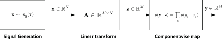
Figure 1: Generalized linear models (GLM)[24].

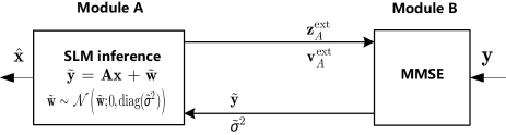
Figure 2: A unified inference framework for GLM.

Specifically, in the $t$-th iteration, the inputs $z_{a,A}^{\textrm{ext}}(t-1)$ and $v_{a,A}^{\textrm{ext}}(t-1)$ to module B are treated as the prior mean and variance of $z_{a}$, respectively. Assuming the prior is Gaussian, the posterior mean and variance of $z_{a}$ can be computed in module B by component-wise MMSE estimate, i.e.,

$$z_{a,B}^{\textrm{post}}(t) =\mathsf{E}(z_{a}|z_{a,A}^{\textrm{ext}}(t-1),v_{a,A}^{\textrm{ext}}(t-1)),$$ (3)

$$v_{a,B}^{\textrm{post}}(t) =\mathsf{Var}(z_{a}|z_{a,A}^{\textrm{ext}}(t-1),v_{a,A}^{\textrm{ext}}(t-1)),$$ (4)

where the expectation is taken w.r.t. the posterior distribution

$$q_{z}^{t-1}\left(z_{a}\right)\propto p\bigl{(}y_{a}|z_{a}\bigr{)}\mathcal{N}\bigl{(}z_{a};z_{a,A}^{\textrm{ext}}(t-1),v_{a,A}^{\textrm{ext}}(t-1)\bigr{)}.$$ (5)

According to the turbo principle [28], the posterior mean and variance cannot be directly used as the output message since they incorporate information of the input messages. Instead, the so-called extrinsic mean $\tilde{y}_{a}(t)$ and variance $\tilde{\sigma}_{a}^{2}(t)$ of $z_{a}$ are calculated by excluding the contribution of input messages $z_{a,A}^{\textrm{ext}}(t-1)$ and $v_{a,A}^{\textrm{ext}}(t-1)$, which are given as [29]

$$\tilde{\sigma}_{a}^{2}(t) =\Bigl{(}\frac{1}{v_{a,B}^{\textrm{post}}(t)}-\frac{1}{v_{a,A}^{\textrm{ext}}(t-1)}\Bigr{)}^{-1},$$ (6)

$$\tilde{y}_{a}(t) =\tilde{\sigma}_{a}^{2}(t)\Bigl{(}\frac{z_{a,B}^{\textrm{post}}(t)}{v_{a,B}^{\textrm{post}}(t)}-\frac{z_{a,A}^{\textrm{ext}}(t-1)}{v_{a,A}^{\textrm{ext}}(t-1)}\Bigr{)}.$$ (7)

For more details of the turbo principle and extrinsic information, please refer to [28, 30]. Then in module A, similar as [30], $\tilde{y}_{a}(t)$ can be viewed as the pseudo-observation of an equivalent additive Gaussian channel with $z_{a}$ as input, i.e.,

$$\tilde{y}_{a}(t)=z_{a}+\tilde{w}_{a}(t),$$ (8)

where $\tilde{w}_{a}(t)\sim\mathcal{N}\bigl{(}\tilde{w}_{a}(t);0,\tilde{\sigma}_{a}^{2}(t)\bigr{)}$. In matrix form, (8) can be rewritten as an SLM form

$$\mathbf{\tilde{y}}(t)=\mathbf{Ax}+\mathbf{\tilde{w}}(t),$$ (9)

where $\mathbf{\tilde{w}}(t)\sim\mathcal{N}\bigl{(}\mathbf{\tilde{w}}(t);\mathbf{0},\mathsf{diag}(\tilde{\boldsymbol{\sigma}}^{2}(t))\bigr{)}$. The underlying theme in (8) is to approximate the estimation error ($\tilde{y}_{a}(t)-z_{a}$) as Gaussian noise whose mean is zero and variance is the extrinsic variance $\tilde{\sigma}_{a}^{2}(t)$. Such idea was first used (to our knowledge) in [30] (formula (47) in [30]). Rigorous theoretical analysis on this will be future work.

As a result, the original GLM problem reduces to an SLM problem so that one can estimate $\mathbf{x}$ by performing SLM inference over (9) to obtain the posterior estimates. Specially, if GLM itself reduces to SLM, then from (6) and (7), we obtain $\tilde{y}_{a}(t)=y_{a}$, $\tilde{\sigma}_{a}^{2}(t)=\sigma^{2}$, which is exactly the original SLM problem. Given the posterior mean and variance estimates of $x_{i}$, the posterior mean $z_{a,A}^{\textrm{post}}(t)$ and variance $v_{a,A}^{\textrm{post}}(t)$ of $z_{a}$ can be obtained using the constraint $\mathbf{z}=\mathbf{Ax}$. Note that the specific method to calculate $z_{a,A}^{\textrm{post}}(t)$ and $v_{a,A}^{\textrm{post}}(t)$ may vary for different SLM inference methods, as shown in Section IV. Given $z_{a,A}^{\textrm{post}}(t)$ and $v_{a,A}^{\textrm{post}}(t)$, the extrinsic mean $z_{a,A}^{\textrm{ext}}(t)$ and variance $v_{a,A}^{\textrm{ext}}(t)$ of $z_{a}$ can be computed as [29]

$$v_{a,A}^{\textrm{ext}}(t) =\Bigl{(}\frac{1}{v_{a,A}^{\textrm{post}}(t)}-\frac{1}{\tilde{\sigma}_{a}^{2}(t)}\Bigr{)}^{-1},$$ (10)

$$z_{a,A}^{\textrm{ext}}(t) =v_{a,A}^{\textrm{ext}}(t)\Bigl{(}\frac{z_{a,A}^{\textrm{post}}(t)}{v_{a,A}^{\textrm{post}}(t)}-\frac{\tilde{y}_{a}(t)}{\tilde{\sigma}_{a}^{2}(t)}\Bigr{)},$$ (11)

which then form the input messages to module B in the next iteration. Note that (10) - (11) and (6) - (7) apply the same rule but are different operations in different modules.

This process continues until convergence or some predefined stopping criteria is satisfied. The corresponding algorithm framework is shown in Algorithm 1. Note that in step 3), one or more iterations can be performed for iterative SLM methods. Under such framework, a variety of inference methods for SLM can be easily extended to GLM. As specific instances, we will show in Section IV how AMP, VAMP, and SBL can be extended to GLM within this framework.

Algorithm 1 Unified framework for GLM inference

1) Initialization: $\mathbf{z}_{A}^{\textrm{ext}}(0),\mathbf{v}_{A}^{\textrm{ext}}(0)$, $t=1$;

2) Update $\tilde{\boldsymbol{\sigma}}^{2}(t)$, $\mathbf{\tilde{y}}(t)$ as (6) and (7);

3) Perform SLM inference over $\mathbf{\tilde{y}}(t)=\mathbf{Ax}+\mathbf{\tilde{w}}(t)$, $\mathbf{\tilde{w}}(t)\sim\mathcal{N}\bigl{(}\mathbf{\tilde{w}}(t);0,\mathsf{diag}(\tilde{\boldsymbol{\sigma}}^{2}(t))\bigr{)}$ via one SLM inference method;

4) Update $\mathbf{v}_{A}^{\textrm{ext}}(t)$, $\mathbf{z}_{A}^{\textrm{ext}}(t)$ as (10) and (11);

5) Set $t\leftarrow t+1$ and proceed to step 2) until $t>T_{max}$.

IV Extending AMP, VAMP, and SBL to GLM

IV-A From AMP to Gr-AMP and GAMP

First review AMP for SLM. Many variants of AMP exist and in this letter we adopt the Bayesian version in [23] and [4]. Assuming the prior distribution $p_{0}\bigl{(}\mathbf{x}\bigr{)}=\prod_{i}p_{0}(x_{i})$, the factor graph for SLM (2) is shown in Fig. 3 (a), where $f_{a}$ denotes the Gaussian distribution $\mathcal{N}\bigl{(}y_{a};\sum_{i=1}^{N}A_{ai}x_{i},\sigma^{2}\bigr{)}$. Denote by $m_{i\rightarrow f_{a}}^{t}(x_{i})=p_{0}(x_{i})\prod_{b\neq a}m_{f_{b}\rightarrow x_{i}}^{t-1}(x_{i})$ the message from $x_{i}$ to $f_{a}$ in the $t$-th iteration, with mean and variance of $x_{i}$ being $\hat{x}_{i\rightarrow a}^{t}$ and $\tau_{i\rightarrow a}^{t}$. Then the message from $f_{a}$ to $x_{i}$ is $m_{f_{a}\rightarrow x_{i}}^{t}(x_{i})=\int\mathcal{N}\bigl{(}y_{a};\sum_{i=1}^{N}A_{ai}x_{i},\sigma^{2}\bigr{)}\prod_{j\neq i}m_{j\rightarrow f_{a}}^{t}(x_{j})dx_{j}$, with mean and variance of $x_{i}$ being $\hat{x}_{a\rightarrow i}^{t}$ and $\tau_{a\rightarrow i}^{t}$, respectively. Define

$$\Sigma_{i}(t) \triangleq\bigl{(}\sum_{a}\frac{1}{\tau_{a\rightarrow i}^{t}}\bigr{)}^{-1},r_{i}(t)\triangleq\Sigma_{i}(t)\bigl{(}\sum_{a}\frac{\hat{x}_{a\rightarrow i}^{t}}{\tau_{a\rightarrow i}^{t}}\bigr{)}^{-1},$$ (12)

$$Z_{a}(t) \triangleq\sum_{i}A_{ai}\hat{x}_{i\rightarrow a}^{t},\;\;V_{a}(t)\triangleq\sum_{i}A_{ai}^{2}\tau_{i\rightarrow a}^{t}.$$ (13)

By the central limit theorem and neglecting high order terms, the resultant AMP is shown in Algorithm 2. Note that the approximation in AMP is asymptotically exact in large system limit, i.e., $N,M\rightarrow\infty$ with $M/N\rightarrow\delta$ [23, 4]. The expectation operation in the posterior mean $\mathsf{E}(x_{i}|r_{i}(t-1),\Sigma_{i}(t-1))$ and variance $\mathsf{Var}(x_{i}|r_{i}(t-1),\Sigma_{i}(t-1))$ in line (D3) and (D4) are w.r.t. the posterior distribution $q_{x}^{t}\left(x_{i}\right)\propto p_{0}(x_{i})\mathcal{N}\bigl{(}x_{i};r_{i}(t),\Sigma_{i}(t)\bigr{)}.$ For more details, refer to [23, 4].

Algorithm 2 AMP Algorithm [23][4]

1) Initialization: $\hat{x}_{i}(0)$,$V_{a}(0),Z_{a}(0)$, $t=1$;

2) Variable node update: For $i=1,...,N$

$${\scriptstyle\Sigma_{i}(t-1)} {\scriptstyle=\Bigl{[}\sum_{a}\frac{A_{ai}^{2}}{\sigma^{2}+V_{a}(t-1)}\Bigr{]}^{-1},}\qquad\qquad\quad\;\qquad\quad\;\;(\textrm{D}1)$$

$${\scriptstyle r_{i}(t-1)} {\scriptstyle=\hat{x}_{i}(t-1)+\Sigma_{i}(t-1)\sum_{a}\frac{A_{ai}\bigl{(}y_{a}-Z_{a}(t-1)\bigr{)}}{\sigma^{2}+V_{a}(t-1)},}\qquad\,(\textrm{D}2)$$

$${\scriptstyle\hat{x}_{i}(t)} {\scriptstyle=\mathsf{E}(x_{i}|r_{i}(t-1),\Sigma_{i}(t-1)),}\>\qquad\qquad\qquad\qquad\,(\textrm{D}3)$$

$${\scriptstyle\tau_{i}(t)} {\scriptstyle=\mathsf{Var}(x_{i}|r_{i}(t-1),\Sigma_{i}(t-1)).}\>\qquad\qquad\qquad\quad\;\,(\textrm{D}4)$$

3) Factor node update: For $a=1,\ldots,M$

$${\displaystyle{\scriptstyle V_{a}(t)}} {\scriptstyle=\sum_{i}A_{ai}^{2}\tau_{i}(t),}{\textstyle\textrm{ }}\qquad\qquad\qquad\qquad\quad\;\;\;\qquad\,\;(\textrm{D}5)$$

$${\scriptstyle Z_{a}(t)} {\scriptscriptstyle=}{\scriptstyle\sum_{i}A_{ai}\hat{x}_{i}(t)-\frac{V_{a}(t)\bigl{(}y_{a}-Z_{a}(t-1)\bigr{)}}{\sigma^{2}+V_{a}(t-1)}.}\qquad\;\;\,\,\qquad\;(\textrm{D}6)$$

4) Set $t\leftarrow t+1$ and proceed to step 2) until $t>\textrm{Iter}{}_{SLM}$.

Then we show how to extend AMP to GLM under the unified framework in Section III. As shown in Algorithm 1, the key lies in calculating the extrinsic mean $\mathbf{z}_{A}^{\textrm{ext}}$ and extrinsic variance $\mathbf{v}_{A}^{\textrm{ext}}$. For AMP, fortunately, these two values have already been calculated, as shown in Lemma 1.

Lemma 1.

After performing AMP in module A, the output extrinsic mean $\mathbf{z}_{A}^{\textrm{ext}}$ and variance $\mathbf{v}_{A}^{\textrm{ext}}$ to module B can be computed as

$$z_{a,A}^{\textrm{ext}}(t)=Z_{a}(t),\quad v_{a,A}^{\textrm{ext}}(t)=V_{a}(t)$$ , (14)

where $Z_{a}(t)$, $V_{a}(t)$ are the results of AMP in line (D6) and (D5) of Algorithm 2, respectively.

Proof:

From (10) and (11), the posterior mean $z_{a,A}^{\textrm{post}}(t)$ and variance $v_{a,A}^{\textrm{post}}(t)$ of $z_{a}$ are needed to calculate $z_{a,A}^{\textrm{ext}}(t)$ and $v_{a,A}^{\textrm{ext}}(t)$. However, in original AMP, they are not explicitly given. To this end, we present an alternative factor graph for SLM in Fig. 3 (b), where $\delta_{a}$ denotes the Dirac function $\delta\bigl{(}z_{a}-\sum_{i=1}^{N}A_{ai}x_{i}\bigr{)}$ and $g_{a}$ denotes Gaussian distribution $\mathcal{N}\bigl{(}z_{a};\tilde{y}_{a}(t),\tilde{\sigma}_{a}^{2}(t)\bigr{)}$. The two factor graph representations in Fig. 3 are equivalent so that the message from $x_{i}$ to $\delta_{a}$ is precisely $m_{i\rightarrow\delta_{a}}^{t}(x_{i})=m_{i\rightarrow f_{a}}^{t}(x_{i})$. Thus, the message from $\delta_{a}$ to $z_{a}$ is $m_{\delta_{a}\rightarrow z_{a}}^{t}(z_{a})=\int\delta\bigl{(}z_{a}-\sum_{i=1}^{N}A_{ai}x_{i}\bigr{)}\prod_{i}m_{i\rightarrow f_{a}}^{t}(x_{i})dx_{i}.$ Recall the definitions of $Z_{a}(t)$ and $V_{a}(t)$ in (13). As in AMP, according to the central limit theorem, $z_{a}=\sum_{i}A_{ai}x_{i}$ can be approximated as Gaussian random variable whose mean and variance are $Z_{a}(t)$ and $V_{a}(t)$, i.e., $m_{\delta_{a}\rightarrow z_{a}}^{t}(z_{a})=\mathcal{N}\bigl{(}z_{a};Z_{a}(t),V_{a}(t)\bigr{)}$. Since the message from $g_{a}$ to $z_{a}$ is $m_{g_{a}\rightarrow z_{a}}^{t}(z_{a})=\mathcal{N}\bigl{(}z_{a};\tilde{y}_{a}(t),\tilde{\sigma}_{a}^{2}(t)\bigr{)}$, the posterior distribution of $z_{a}$ can be calculated as $q^{t}(z_{a})\propto m_{\delta_{a}\rightarrow z_{a}}^{t}(z_{a})m_{g_{a}\rightarrow z_{a}}^{t}(z_{a})\propto\mathcal{N}\bigl{(}z_{a};z_{a,A}^{\textrm{post}}(t),v_{a,A}^{\textrm{post}}(t)\bigr{)},$ where

$$v_{a,A}^{\textrm{post}}(t) =\Bigl{(}\frac{1}{V_{a}(t)}+\frac{1}{\tilde{\sigma}_{a}^{2}(t)}\Bigr{)}^{-1},$$ (15)

$$z_{a,A}^{\textrm{post}}(t) =v_{a,A}^{\textrm{post}}(t)\Bigl{(}\frac{Z_{a}(t)}{V_{a}(t)}+\frac{\tilde{y}_{a}(t)}{\tilde{\sigma}_{a}^{2}(t)}\Bigr{)}.$$ (16)

Substituting (15), (16) into (10), (11), we obtain $v_{a,A}^{\textrm{ext}}(t)=V_{a}(t)$ and $z_{a,A}^{\textrm{ext}}(t)=Z_{a}(t)$. In the derivation of AMP [23, 4], $V_{a}(t)$ and $Z_{a}(t)$ are computed as (D5) and (D6) of Algorithm 2 in large system limit, which completes the proof. ∎

      

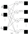
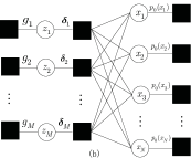
Figure 3: Two equivalent factor graph representations of SLM.

According to Lemma 1 and the framework in Algorithm 1, we readily obtain a generalized version of AMP called Gr-AMP, as shown in Algorithm 3.

Algorithm 3 Generalized version of AMP (Gr-AMP)

1) Initialization: $\mathbf{z}_{A}^{\textrm{ext}}(0),\mathbf{v}_{A}^{\textrm{ext}}(0)$, $t=1$;

2) Update $\tilde{\boldsymbol{\sigma}}^{2}(t)$, $\mathbf{\tilde{y}}(t)$ as (6) and (7);

3) Perform AMP with $\textrm{Iter}{}_{SLM}$ iterations over $\mathbf{\tilde{y}}(t)=\mathbf{Ax}+\mathbf{\tilde{w}}(t)$, $\mathbf{\tilde{w}}(t)\sim\mathcal{N}\bigl{(}\mathbf{\tilde{w}}(t);\mathbf{0},\mathsf{diag}(\tilde{\boldsymbol{\sigma}}^{2}(t))\bigr{)}$ and update $v_{a,A}^{\textrm{ext}}(t)=V_{a}(t)$, $z_{a,A}^{\textrm{ext}}(t)=Z_{a}(t)$ with the results of AMP.

4) Set $t\leftarrow t+1$ and proceed to step 2) until $t>T_{\textrm{max}}$.

Note that the proposed Gr-AMP in Algorithm 3 can be viewed as a general form of the well-known GAMP [23]. In particular, if $\textrm{Iter}{}_{SLM}=1$, Gr-AMP becomes equivalent to the original GAMP. To prove this, in step 2) of Algorithm 3, we first obtain the equivalent noise variance $\tilde{\sigma}_{a}^{2}(t)$ and observation $\tilde{y}_{a}(t)$ from (6) and (7) with $v_{a,A}^{\textrm{ext}}(t-1)=V_{a}(t-1)$ and $z_{a,A}^{\textrm{ext}}(t-1)=Z_{a}(t-1)$. Then, in step 3) of Algorithm 3, one iteration of AMP is performed by simply replacing $\sigma^{2}$, $y_{a}$ in Algorithm 2 with $\tilde{\sigma}_{a}^{2}(t)$, $\tilde{y}_{a}(t)$. After some algebra and the definitions of two intermediate variables $\hat{s}_{a}(t-1)$ and $\tau_{a}^{s}(t-1)$ in (17) and (18), the $t$-th iteration of the proposed Gr-AMP in Algorithm 3 with $\textrm{Iter}{}_{SLM}=1$ becomes

$$\hat{s}_{a}(t-1) =\frac{z_{a,B}^{\textrm{post}}(t)-Z_{a}(t-1)}{V_{a}(t-1)},$$ (17)

$$\tau_{a}^{s}(t-1) =\frac{V_{a}(t-1)-v_{a,B}^{\textrm{post}}(t)}{V_{a}^{2}(t-1)},$$ (18)

$$\Sigma_{i}(t-1) =\Bigl{[}\sum_{a}A_{ai}^{2}\tau_{a}^{s}(t-1)\Bigr{]}^{-1},$$ (19)

$$r_{i}(t-1) =\hat{x}_{i}(t-1)+\Sigma_{i}(t-1)\sum_{a}A_{ai}\hat{s}_{a}(t-1),$$ (20)

$$\hat{x}_{i}(t) =\mathsf{E}(x_{i}|r_{i}(t-1),\Sigma_{i}(t-1)),$$ (21)

$$\tau_{i}(t) =\mathsf{Var}(x_{i}|r_{i}(t-1),\Sigma_{i}(t-1)),$$ (22)

$$V_{a}(t) =\sum_{i}A_{ai}^{2}\tau_{i}(t),$$ (23)

$$Z_{a}(t) =\sum_{i}A_{ai}\hat{x}_{i}(t)-V_{a}(t)\hat{s}_{a}(t-1).$$ (24)

Recalling the definitions (3) and (4), it can be seen that Gr-AMP with $\textrm{Iter}{}_{SLM}=1$ is equivalent to the original GAMP [23, 24]. As a result, the proposed framework provides a new perspective on GAMP and leads to a concise derivation.

IV-B From VAMP and SBL to Gr-VAMP and Gr-SBL

For VAMP and SBL, the values of $\mathbf{z}_{A}^{\textrm{ext}}$ and $\mathbf{v}_{A}^{\textrm{ext}}$ are not already calculated as in AMP. However, the posterior mean and covariance matrix of $\mathbf{x}$, denoted as $\mathbf{\hat{x}}_{2k}$ and $\mathbf{C}_{2k}$, respectively, can be obtained in the linear MMSE (LMMSE) operation of VAMP and SBL (refer to [13], [25], and [26]). Thus, the posterior mean and variance of $\mathbf{z}$ are calculated as $\mathbf{z}_{A}^{\textrm{post}}=\mathbf{A}\mathbf{\hat{x}}_{2k}$, $\mathbf{v}_{A}^{\textrm{post}}=\frac{1}{M}\mathsf{trace}(\mathbf{A}\mathbf{C}_{2k}\mathbf{A}^{T})$, where $\mathsf{trace}(\mathbf{X})$ denotes the trace of matrix $\mathbf{X}$. Then, we obtain $\mathbf{z}_{A}^{\textrm{ext}}$ and variance $\mathbf{v}_{A}^{\textrm{ext}}$ from (10) and (11). The resulting generalized VAMP (Gr-VAMP) and generalized SBL (Gr-SBL) are shown in Algorithm 4.

Algorithm 4 Generalized VAMP/SBL (Gr-VAMP/Gr-SBL)

1) Initialization: $\mathbf{z}_{A}^{\textrm{ext}}(0),\mathbf{v}_{A}^{\textrm{ext}}(0)$, $t=1$;

2) Update $\tilde{\boldsymbol{\sigma}}^{2}(t)$, $\mathbf{\tilde{y}}(t)$ as (6) and (7);

3) Perform VAMP/SBL with $\textrm{Iter}{}_{SLM}$ iterations over $\mathbf{\tilde{y}}(t)=\mathbf{Ax}+\mathbf{\tilde{w}}(t)$, $\mathbf{\tilde{w}}(t)\sim\mathcal{N}\bigl{(}\mathbf{\tilde{w}}(t);\mathbf{0},\mathsf{diag}(\tilde{\boldsymbol{\sigma}}^{2}(t))\bigr{)}$;

4) Update $\mathbf{v}_{A}^{\textrm{ext}}(t)$, $\mathbf{z}_{A}^{\textrm{ext}}(t)$ as (10) and (11) with $\mathbf{z}_{A}^{\textrm{post}}(t)=\mathbf{A}\mathbf{\hat{x}}_{2k}(t)$, $\mathbf{v}_{A}^{\textrm{post}}(t)=\frac{1}{M}\mathsf{trace}(\mathbf{A}\mathbf{C}_{2k}(t)\mathbf{A}^{T})$, where $\mathbf{\hat{x}}_{2k}(t)$ and $\mathbf{C}_{2k}(t)$ are the posterior mean and covariance matrix obtained in the LMMSE step of VAMP/SBL, respectively.

5) Set $t\leftarrow t+1$ and proceed to step 2) until $t>T_{\textrm{max}}$.

IV-C Applications to 1-bit Compressed Sensing

In this subsection, we evaluate the performances of Gr-AMP, Gr-VAMP, and Gr-SBL for 1-bit CS. Assume that the sparse signal $\mathbf{x}$ follows i.i.d. Bernoulli-Gaussian distribution $p_{0}\bigl{(}\mathbf{x}\bigr{)}=\prod_{i}\bigl{(}1-\rho\bigr{)}\delta\bigl{(}x_{i}\bigr{)}+\rho\mathcal{N}\bigl{(}x_{i};0,\rho^{-1}\bigr{)}$. The 1-bit quantized measurements are obtained by $\mathbf{y}=\mathtt{\mathsf{sign}}\left(\mathbf{Ax}+\mathbf{w}\right)$, where $\mathtt{\mathsf{sign}}(\cdot)$ is the component-wise sign of each element. We consider the case $N=512,M=2048$ for sparse ratio $\rho=0.1$. The signal to noise ratio (SNR) $\mathsf{E}(\left\|\mathbf{Ax}\right\|_{2}^{2})/\mathsf{E}(\left\|\mathbf{w}\right\|_{2}^{2})$ is set to be 50 dB. To test the performances for general matrix $\mathbf{A}$, ill-conditioned matrices with various condition numbers are considered following [13]. Specifically, $\mathbf{A}$ is constructed from the singular value decomposition (SVD) $\mathbf{A}=\mathbf{US}\mathbf{V}^{T}$, where orthogonal matrices $\mathbf{U}$ and $\mathbf{V}$ were uniformly drawn w.r.t. Harr measure. The singular values were chosen to achieve a desired condition number $\kappa(\mathbf{A})=\lambda_{\textrm{max}}/\lambda_{\textrm{min}}$, where $\lambda_{\textrm{max}}$ and $\lambda_{\textrm{min}}$ are the maximum and minimum singular values of $\mathbf{A}$, respectively. As in [14], the recovery performance is assessed using the debiased normalized mean square error (dNMSE) in decibels, i.e.,$\underset{c}{\textrm{min}}\>20\log_{10}(\left\|c\mathbf{\hat{x}}-\mathbf{x}\right\|_{2}/\left\|\mathbf{x}\right\|_{2})$. In all simulations, $\textrm{Iter}{}_{SLM}=1,T_{\textrm{max}}=50,\mathbf{z}_{A}^{\textrm{ext}}(0)=0,\mathbf{v}_{A}^{\textrm{ext}}(0)=10^{8}$ and the results are averaged over 100 realizations. The results of GAMP and the algorithm in [14], denoted as GVAMP, are also given for comparison.

Fig. 4 (a) and (b) show the results of dNMSE versus the number of algorithm iterations when the condition number $\kappa(\mathbf{A})=1\textrm{ and }100$, respectively. When $\kappa(\mathbf{A})=1$, all algorithms converge to the same dNMSE value except Gr-SBL which has slightly worse performance. When $\kappa(\mathbf{A})=100$, however, both Gr-AMP and GAMP fail while other algorithms still work well. In Fig. 4 (c), the dNMSE is evaluated for various condition number $\kappa(\mathbf{A})$ ranging from 1 (i.e., row-orthogonal matrix $\mathbf{A}$) to $1\times 10^{6}$ (i.e., highly ill-conditioned matrix $\mathbf{A}$). It is seen that as the condition number $\kappa(\mathbf{A})$ increases, the recovery performances degrade smoothly for Gr-VAMP, GVAMP, and Gr-SBL while both Gr-AMP and GAMP diverge for even mild condition number.

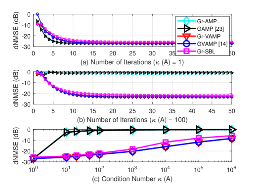
Figure 4: dNMSE versus number of iterations for (a): $\kappa(\mathbf{A})$= 1 and (b): $\kappa(\mathbf{A})$= 100; (c) dNMSE versus the condition number $\kappa(\mathbf{A})$.

V Conclusion

In this letter a unified Bayesian inference framework for GLM is presented whereby a variety of SLM algorithms can be easily extended to handle the GLM problem. Specific instances elucidated under this framework are the extensions of AMP, VAMP, and SBL, which unveils intimate connections between some established algorithms and leads to novel extensions for some other SLM algorithms. Numerical results for 1-bit CS demonstrate the effectiveness of this framework.

References

- [1] D. L. Donoho, A. Maleki, and A. Montanari, “Message-passing algorithms for compressed sensing,” in Proc. Nat. Acad. Sci., vol. 106, no. 45, Nov. 2009, pp. 18 914–18 919.
- [2] E. J. Candès and M. B. Wakin, “An introduction to compressive sampling,” IEEE Signal Process. Mag., vol. 25(2), pp. 21–30, Mar. 2008.
- [3] D. L. Donoho, A. Maleki, and A. Montanari, “Message passing algorithms for compressed sensing: I. motivation and construction,” in IEEE Information Theory Workshop (ITW), Jan. 2010, pp. 1–5.
- [4] F. Krzakala, M. Mézard, F. Sausset, Y. Sun, and L. Zdeborová, “Probabilistic reconstruction in compressed sensing: algorithms, phase diagrams, and threshold achieving matrices,” Journal of Statistical Mechanics: Theory and Experiment, vol. 2012, no. 08, p. P08009, 2012.
- [5] S. Som and P. Schniter, “Compressive imaging using approximate message passing and a markov-tree prior,” IEEE Trans. Signal Process., vol. 60, no. 7, pp. 3439–3448, 2012.
- [6] J. P. Vila and P. Schniter, “Expectation-maximization Gaussian-mixture approximate message passing,” IEEE Trans. Signal Process., vol. 61, no. 19, pp. 4658–4672, 2013.
- [7] J. Ziniel and P. Schniter, “Dynamic compressive sensing of time-varying signals via approximate message passing,” IEEE Trans. Signal Process., vol. 61, no. 21, pp. 5270–5284, 2013.
- [8] ——, “Efficient high-dimensional inference in the multiple measurement vector problem,” IEEE Trans. Signal Process., vol. 61, no. 2, pp. 340–354, 2013.
- [9] S. Wu, L. Kuang, Z. Ni, J. Lu, D. Huang, and Q. Guo, “Low-complexity iterative detection for large-scale multiuser MIMO-OFDM systems using approximate message passing,” IEEE J. Sel. Topics Signal Process., vol. 8, no. 5, pp. 902–915, Oct. 2014.
- [10] X. Meng, S. Wu, L. Kuang, and J. Lu, “An expectation propagation perspective on approximate message passing,” IEEE Signal Processing Letters, vol. 22, no. 8, pp. 1194–1197, 2015.
- [11] S. Wang, Y. Li, and J. Wang, “Multiuser detection in massive spatial modulation MIMO with low-resolution ADCs,” IEEE Trans. Wireless Commun., vol. 14, no. 4, pp. 2156–2168, 2015.
- [12] J. Ma, X. Yuan, and L. Ping, “Turbo compressed sensing with partial DFT sensing matrix,” IEEE Signal Processing Letters, vol. 22, no. 2, pp. 158–161, 2014.
- [13] S. Rangan, P. Schniter, and A. Fletcher, “Vector approximate message passing,” arXiv:1610.03082, 2016.
- [14] P. Schniter, S. Rangan, and A. K. Fletcher, “Vector approximate message passing for the generalized linear model,” in 2016 50th Asilomar Conference on Signals, Systems and Computers, Nov 2016, pp. 1525–1529.
- [15] P. Schniter, S. Rangan, and A. Fletcher, “Denoising based vector approximate message passing,” arXiv:1611.01376, 2016.
- [16] Z. Xue, J. Ma, and X. Yuan, “D-OAMP: A denoising-based signal recovery algorithm for compressed sensing,” in 2016 IEEE Global Conference on Signal and Information Processing (GlobalSIP), 2016.
- [17] J. Ma and L. Ping, “Orthogonal AMP,” IEEE Access, vol. 5, no. 99, pp. 2020–2033, 2016.
- [18] T. Liu, C. K. Wen, S. Jin, and X. You, “Generalized turbo signal recovery for nonlinear measurements and orthogonal sensing matrices,” in 2016 IEEE International Symposium on Information Theory (ISIT), 2016, pp. 2883–2887.
- [19] H. He, C. K. Wen, and S. Jin, “Generalized expectation consistent signal recovery for nonlinear measurements,” in 2017 IEEE International Symposium on Information Theory (ISIT), June 2017, pp. 2333–2337.
- [20] U. S. Kamilov, V. K. Goyal, and S. Rangan, “Message-passing de-quantization with applications to compressed sensing,” IEEE Transactions on Signal Processing, vol. 60, no. 12, pp. 6270–6281, 2012.
- [21] C. M. Bishop, Pattern recognition and machine learning. New York: Springer, 2006.
- [22] K. Jaganathan, Y. C. Eldar, and B. Hassibi, “Phase retrieval: An overview of recent developments,” Mathematics, 2015.
- [23] S. Rangan, “Generalized approximate message passing for estimation with random linear mixing,” in Proc. IEEE Int. Symp. Inf. Theory, 2011, pp. 2168–2172.
- [24] ——, “Generalized approximate message passing for estimation with random linear mixing,” arXiv:1010.5141v2, 2012.
- [25] M. E. Tipping, “Sparse Bayesian learning and the relevance vector machine,” The journal of machine learning research, vol. 1, pp. 211–244, 2001.
- [26] D. P. Wipf and B. D. Rao, “Sparse Bayesian learning for basis selection,” IEEE Trans. Signal Process., vol. 52, no. 8, pp. 2153–2164, 2004.
- [27] P. Marttinen, J. Gillberg, A. Havulinna, J. Corander, and S. Kaski, “Approximate bayesian computation (ABC) gives exact results under the assumption of model error,” Statistical Applications in Genetics & Molecular Biology, vol. 12, no. 2, pp. 129–141, 2013.
- [28] C. Berrou and A. Glavieux, “Near optimum error correcting coding and decoding: Turbo-codes,” IEEE Trans.Commun., vol. 44, no. 10, pp. 1261–1271, 1996.
- [29] Q. Guo and D. D. Huang, “A concise representation for the soft-in soft-out LMMSE detector,” IEEE Commun. Lett., vol. 15, no. 5, pp. 566–568, May 2011.
- [30] X. Wang and H. V. Poor, “Iterative (turbo) soft interference cancellation and decoding for coded CDMA,” IEEE Trans. Commun., vol. 47, no. 7, pp. 1046–1061, July 1999.