SBEED: Convergent Reinforcement Learning with Nonlinear Function Approximation

Abstract

When function approximation is used, solving the Bellman optimality equation with stability guarantees has remained a major open problem in reinforcement learning for decades. The fundamental difficulty is that the Bellman operator may become an expansion in general, resulting in oscillating and even divergent behavior of popular algorithms like Q-learning. In this paper, we revisit the Bellman equation, and reformulate it into a novel primal-dual optimization problem using Nesterov’s smoothing technique and the Legendre-Fenchel transformation. We then develop a new algorithm, called Smoothed Bellman Error Embedding, to solve this optimization problem where any differentiable function class may be used. We provide what we believe to be the first convergence guarantee for general nonlinear function approximation, and analyze the algorithm’s sample complexity. Empirically, our algorithm compares favorably to state-of-the-art baselines in several benchmark control problems.

1 Introduction

In reinforcement learning (RL), the goal of an agent is to learn a policy that maximizes long-term returns by sequentially interacting with an unknown environment (Sutton & Barto, 1998). The dominating framework to model such an interaction is the Markov decision process, or MDP, in which the optimal value function are characterized as a fixed point of the Bellman operator. A fundamental result for MDP is that the Bellman operator is a contraction in the value-function space, so the optimal value function is the unique fixed point. Furthermore, starting from any initial value function, iterative applications of the Bellman operator ensure convergence to the fixed point. Interested readers are referred to the textbook of Puterman (2014) for details.

Many of the most effective RL algorithms have their root in such a fixed-point view. The most prominent family of algorithms is perhaps the temporal-difference algorithms, including TD$(\lambda)$ (Sutton, 1988), Q-learning (Watkins, 1989), SARSA (Rummery & Niranjan, 1994; Sutton, 1996), and numerous variants such as the empirically very successful DQN (Mnih et al., 2015) and A3C (Mnih et al., 2016) implementations. Compared to direct policy search/gradient algorithms like REINFORCE (Williams, 1992), these fixed-point methods make learning more efficient by bootstrapping (a sample-based version of Bellman operator).

When the Bellman operator can be computed exactly (even on average), such as when the MDP has finite state/actions, convergence is guaranteed thanks to the contraction property (Bertsekas & Tsitsiklis, 1996). Unfortunately, when function approximatiors are used, such fixed-point methods easily become unstable or even divergent (Boyan & Moore, 1995; Baird, 1995; Tsitsiklis & Van Roy, 1997), except in a few special cases. For example,

• for some rather restrictive function classes, such as those with a non-expansion property, some of the finite-state MDP theory continues to apply with modifications (Gordon, 1995; Ormoneit & Sen, 2002; Antos et al., 2008);

• when linear value function approximation in certain cases, convergence is guaranteed: for evaluating a fixed policy from on-policy samples (Tsitsiklis & Van Roy, 1997), for evaluating the policy using a closed-form solution from off-policy samples (Boyan, 2002; Lagoudakis & Parr, 2003), or for optimizing a policy using samples collected by a stationary policy (Maei et al., 2010).

In recent years, a few authors have made important progress toward finding scalable, convergent TD algorithms, by designing proper objective functions and using stochastic gradient descent (SGD) to optimize them (Sutton et al., 2009; Maei, 2011). Later on, it was realized that several of these gradient-based algorithms can be interpreted as solving a primal-dual problem (Mahadevan et al., 2014; Liu et al., 2015; Macua et al., 2015; Dai et al., 2016). This insight has led to novel, faster, and more robust algorithms by adopting sophisticated optimization techniques (Du et al., 2017). Unfortunately, to the best of our knowledge, all existing works either assume linear function approximation or are designed for policy evaluation. It remains a major open problem how to find the optimal policy reliably with general nonlinear function approximators such as neural networks, especially in the presence of off-policy data.

Contributions

In this work, we take a substantial step towards solving this decades-long open problem, leveraging a powerful saddle-point optimization perspective, to derive a new algorithm called Smoothed Bellman Error Embedding (SBEED) algorithm. Our development hinges upon a novel view of a smoothed Bellman optimality equation, which is then transformed to the final primal-dual optimization problem. SBEED learns the optimal value function and a stochstic policy in the primal, and the Bellman error (also known as Bellman residual) in the dual. By doing so, it avoids the non-smooth $\max$-operator in the Bellman operator, as well as the double-sample challenge that has plagued RL algorithm designs (Baird, 1995). More specifically,

• SBEED is stable for a broad class of nonlinear function approximators including neural networks, and provably converges to a solution with vanishing gradient. This holds even in the more challenging off-policy case;

• it uses bootstrapping to yield high sample efficiency, as in TD-style methods, and is also generalized to cases of multi-step bootstrapping and eligibility traces;

• it avoids the double-sample issue and directly optimizes the squared Bellman error based on sample trajectories;

• it uses stochastic gradient descent to optimize the objective, thus very efficient and scalable.

Furthermore, the algorithm handles both the optimal value function estimation and policy optimization in a unified way, and readily applies to both continuous and discrete action spaces. We compare the algorithm with state-of-the-art baselines on several continuous control benchmarks, and obtain excellent results.

2 Preliminaries

In this section, we introduce notation and technical background that is needed in the rest of the paper. We denote a Markov decision process (MDP) as $\mathcal{M}=\left({\mathcal{S}},\mathcal{A},P,R,\gamma\right)$, where ${\mathcal{S}}$ is a (possible infinite) state space, $\mathcal{A}$ an action space, $P(\cdot|s,a)$ the transition probability kernel defining the distribution over next states upon taking action $a$ on state $s$, $R(s,a)$ the average immediate reward by taking action $a$ in state $s$, and $\gamma\in(0,1)$ a discount factor. Given an MDP, we wish to find a possibly stochastic policy $\pi:{\mathcal{S}}\to\mathcal{P}_{\mathcal{A}}$ to maximize the expected discounted cumulative reward starting from any state $s\in{\mathcal{S}}$: $\mathbb{E}\left[\sum_{t=0}^{\infty}\gamma^{t}R(s_{t},a_{t})\Big{|}s_{0}=s,\pi\right]$, where $\mathcal{P}_{\mathcal{A}}$ denotes all probability measures over $\mathcal{A}$. The set of all policies is denoted by $\mathcal{P}:=(\mathcal{P}_{\mathcal{A}})^{\mathcal{S}}$.

Define $V^{*}(s):=\max_{\pi(\cdot|s)}\mathbb{E}\left[\sum_{t=0}^{\infty}\gamma^{t}R(s_{t},a_{t})|s_{0}=s,\pi\right]$ to be the optimal value function. It is known that $V^{*}$ is the unique fixed point of the Bellman operator ${\mathcal{T}}$, or equivalently, the unique solution to the Bellman optimality equation (Bellman equation, for short) (Puterman, 2014):

$$V(s)=({\mathcal{T}}V)(s):=\max_{a}\,{R(s,a)+\gamma\mathbb{E}_{s^{\prime}|s,a}\left[V(s^{\prime})\right]}.$$ (1)

The optimal policy $\pi^{*}$ is related to $V^{*}$ by the following:

$$\pi^{*}(a|s)=\mathop{\mathrm{argmax}}_{a}\left\{R(s,a)+\gamma\mathbb{E}_{s^{\prime}|s,a}\left[V^{*}(s^{\prime})\right]\right\}.$$

It should be noted that in practice, for convenience we often work on the Q-function instead of the state-value function $V^{*}$. In this paper, it suffices to use the simpler $V^{*}$ function.

3 A Primal-Dual View of Bellman Equation

In this section, we introduce a novel view of Bellman equation that enables the development of the new algorithm in Section 4. After reviewing the Bellman equation and the challenges to solve it, we describe the two key technical ingredients that lead to our primal-dual reformulation.

We start with another version of Bellman equation that is equivalent to Eqn (1) (see, e.g., Puterman (2014)):

$$V(s)=\max_{\pi(\cdot|s)\in\mathcal{P}_{\mathcal{A}}}\mathbb{E}_{a\sim\pi(\cdot|s)}\left[{R(s,a)}+\gamma\mathbb{E}_{s^{\prime}|s,a}\left[V(s^{\prime})\right]\right].$$ (2)

Eqn (2) makes the role of a policy explicit. Naturally, one may try to jointly optimize over $V$ and $\pi$ to minimize the discrepancy between the two sides of (2). For concreteness, we focus on the square distance in this paper, but our results can be extended to other convex loss functions. Let $\mu$ be some given state distribution so that $\mu(s)>0$ for all $s\in{\mathcal{S}}$. Minimizing the squared Bellman error gives the following:

$$\min_{V}\,\mathbb{E}_{s\sim\mu}\left[\left(\max_{\pi(\cdot|s)\in\mathcal{P}_{\mathcal{A}}}\mathbb{E}_{a\sim\pi(\cdot|s)}\left[R(s,a)+\gamma\mathbb{E}_{s^{\prime}|s,a}\left[V(s^{\prime})\right]\right]-V(s)\right)^{2}\right]\,.$$ (3)

While natural, this approach has several major difficulties when it comes to optimization, which are to be dealt with in the following subsections:

• The $\max$ operator over $\mathcal{P}_{\mathcal{A}}$ introduces non-smoothness to the objective function. A slight change in $V$ may cause large differences in the RHS of Eqn (2).

• The conditional expectation, $\mathbb{E}_{s^{\prime}|s,a}\left[\cdot\right]$, composed within the square loss, requires double samples (Baird, 1995) to obtain unbiased gradients, which is often impractical in most but simulated environments.

3.1 Smoothed Bellman Equation

To avoid the instability and discontinuity caused by the $\max$ operator, we use the smoothing technique of Nesterov (2005) to smooth the Bellman operator ${\mathcal{T}}$. Since policies are conditional distributions over $\mathcal{A}$, we choose entropy regularization, and Eqn (2) becomes:

$$V_{\lambda}(s)=\max_{\pi(\cdot|s)\in\mathcal{P}_{\mathcal{A}}}\Big{(}\mathbb{E}_{a\sim\pi(\cdot|s)}\big{(}R(s,a)+\gamma\mathbb{E}_{s^{\prime}|s,a}\left[V_{\lambda}(s^{\prime})\right]\big{)}+\lambda H(\pi,s)\Big{)}\,,$$ (4)

where $H(\pi,s):=-\sum_{a\in\mathcal{A}}\pi(a|s)\log\pi(a|s)$, and $\lambda\geqslant 0$ controls the degree of smoothing. Note that with $\lambda=0$, we obtain the standard Bellman equation. Moreover, the regularization may be viewed a shaping reward added to the reward function of an induced, equivalent MDP; see Appendix C.2 for more details.

Since negative entropy is the conjugate of the log-sum-exp function (Boyd & Vandenberghe, 2004, Example 3.25), Eqn (4) can be written equivalently as

$$V_{\lambda}(s)=\left({\mathcal{T}}_{\lambda}V_{\lambda}\right)(s):=\lambda\log\left(\sum_{a\in\mathcal{A}}\exp\left(\frac{R(s,a)+\gamma\mathbb{E}_{s^{\prime}|s,a}\left[V_{\lambda}(s^{\prime})\right]}{\lambda}\right)\right)$$ (5)

where the $\log$-sum-$\exp$ is an effective smoothing approximation of the $\max$-operator.

Remark.

While Eqns (4) and (5) are inspired by Nestorov smoothing technique, they can also be derived from other principles (Rawlik et al., 2012; Fox et al., 2016; Neu et al., 2017; Nachum et al., 2017; Asadi & Littman, 2017). For example, Nachum et al. (2017) use entropy regularization in the policy space to encourage exploration, but arrive at the same smoothed form; the smoothed operator ${\mathcal{T}}_{\lambda}$ is called “Mellowmax” by Asadi & Littman (2017), which is obtained as a particular instantiation of the quasi-arithmetic mean. In the rest of the subsection, we review the properties of ${\mathcal{T}}_{\lambda}$, although some of the results have appeared in the literature in slightly different forms. Proofs are deferred to Appendix A.

First, we show ${\mathcal{T}}_{\lambda}$ is also a contraction, as with the standard Bellman operator (Fox et al., 2016; Asadi & Littman, 2017):

Proposition 1 (Contraction)

${\mathcal{T}}_{\lambda}$ is a $\gamma$-contraction. Consequently, the corresponding smoothed Bellman equation (4), or equivalently (5), has a unique solution $V_{\lambda}^{*}$.

Second, we show that while in general $V^{*}\neq V_{\lambda}^{*}$, their difference is controlled by $\lambda$. To do so, define $H^{*}:=\max_{s\in{\mathcal{S}},\pi(\cdot|s)\in\mathcal{P}_{\mathcal{A}}}H(\pi,s)$. For finite action spaces, we immediately have $H^{*}=\log(\left|\mathcal{A}\right|)$.

Proposition 2 (Smoothing bias)

Let $V^{*}$ and $V_{\lambda}^{*}$ be fixed points of (2) and (4), respectively. Then,

$$\left\|V^{*}(s)-V_{\lambda}^{*}(s)\right\|_{\infty}\leqslant\frac{\lambda H^{*}}{1-\gamma}\,.$$

Consequently, as $\lambda\to 0$, $V_{\lambda}^{*}$ converges to $V^{*}$ pointwisely.

Finally, the smoothed Bellman operator has the very nice property of temporal consistency (Rawlik et al., 2012; Nachum et al., 2017):

Proposition 3 (Temporal consistency)

Assume $\lambda>0$. Let $V_{\lambda}^{*}$ be the fixed point of (4) and $\pi_{\lambda}^{*}$ the corresponding policy that attains the maximum on the RHS of (4). Then, $(V_{\lambda}^{*},\pi_{\lambda}^{*})$ is the unique $(V,\pi)$ pair that satisfies the following equality for all $(s,a)\in{\mathcal{S}}\times\mathcal{A}$:

$$V(s)={R(s,a)+\gamma\mathbb{E}_{s^{\prime}|s,a}\left[V(s^{\prime})\right]-\lambda\log\pi(a|s)}\,.$$ (6)

In other words, Eqn (6) provides an easy-to-check condition to characterize the optimal value function and optimal policy on arbitrary pair of $(s,a)$, therefore, which is easy to incorporate off-policy data. It can also be extended to the multi-step or eligibility-traces cases (Appendix C; see also Sutton & Barto (1998, Chapter 7)). Later, this condition will be one of the critical foundations to develop our new algorithm.

3.2 Bellman Error Embedding

A natural objective function inspired by (6) is the mean squared consistency Bellman error, given by:

$$\min_{V,\pi\in\mathcal{P}}\;\ell(V,\pi) := \mathbb{E}_{s,a}\Big{[}\big{(}R(s,a)+\gamma\mathbb{E}_{s^{\prime}|s,a}\left[V(s^{\prime})\right]-\lambda\log\pi(a|s)-V(s)\big{)}^{2}\Big{]}\,,$$ (7)

where $\mathbb{E}_{s,a}[\cdot]$ is shorthand for $\mathbb{E}_{s\sim\mu(\cdot),a\sim\pi_{b}(\cdot|s)}[\cdot]$. Unfortunately, due to the inner conditional expectation, it would require two independent sample of $s^{\prime}$ (starting from the same $(s,a)$) to obtain an unbiased estimate of gradient of $f$, a problem known as the double-sample issue (Baird, 1995). In practice, however, one can rarely obtain two independent samples except in simulated environments.

To bypass this problem, we make use of the conjugate of the square function (Boyd & Vandenberghe, 2004): ${{x}^{2}}=\max_{\nu}\left(2\nu x-\nu^{2}\right)$, as well as the interchangeability principle (Shapiro et al., 2009; Dai et al., 2016) to rewrite the optimization problem (7) into an equivalent form:

$$\min_{V,\pi\in\mathcal{P}}\max_{\nu\in\mathcal{F}_{{\mathcal{S}}\times\mathcal{A}}}L(V,\pi;\nu):=2\mathbb{E}_{s,a,s^{\prime}}\Big{[}\nu(s,a)\big{(}R(s,a)+\gamma{V(s^{\prime})-\lambda\log\pi(a|s)}-V(s)\big{)}\Big{]}-\mathbb{E}_{s,a,s^{\prime}}\left[\nu^{2}(s,a)\right]\,,$$ (8)

where $\mathcal{F}_{{\mathcal{S}}\times\mathcal{A}}$ is the set of real-valued functions on ${\mathcal{S}}\times\mathcal{A}$, $\mathbb{E}_{s,a,s^{\prime}}[\cdot]$ is shorthand for $\mathbb{E}_{s\sim\mu(\cdot),a\sim\pi_{b}(\cdot|s),s^{\prime}\sim P(\cdot|s,a)}[\cdot]$. Note that (8) is not a standard convex-concave saddle-point problem: the objective is convex in $V$ for any fixed $(\pi,\nu)$, and concave in $\nu$ for any fixed $(V,\pi)$, but not necessarily convex in $\pi\in\mathcal{P}$ for any fixed $(V,\nu)$.

Remark.

In contrast to our saddle-point formulation (8), Nachum et al. (2017) get around the double-sample obstacle by minimizing an upper bound of $\ell(V,\pi)$: $\tilde{\ell}(V,\pi):=\mathbb{E}_{s,a,s^{\prime}}\left[\left(R(s,a)+\gamma{V(s^{\prime})}-\lambda\log\pi(a|s)-V(s)\right)^{2}\right]$. As is known (Baird, 1995), the gradient of $\tilde{\ell}$ is different from that of $f$, as it has a conditional variance term coming from the stochastic outcome $s^{\prime}$. In problems where this variance is highly heterogeneous across different $(s,a)$ pairs, impact of such a bias can be substantial.

Finally, substituting the dual function $\nu(s,a)=\rho(s,a)-V(s)$, the objective in the saddle point problem becomes

$$\min_{V,\pi}\max_{\rho\in\mathcal{F}_{{\mathcal{S}}\times\mathcal{A}}}L_{1}(V,\pi;\rho) := \mathbb{E}_{s,a,s^{\prime}}\left[\left(\delta(s,a,s^{\prime})-V(s)\right)^{2}\right]-\mathbb{E}_{s,a,s^{\prime}}\left[\left({\delta(s,a,s^{\prime})}-\rho(s,a)\right)^{2}\right]$$ (9)

where $\delta(s,a,s^{\prime}):=R(s,a)+\gamma{V(s^{\prime})-\lambda\log\pi(a|s)}$. Note that the first term is $\tilde{\ell}(V,\pi)$, and the second term will cancel the extra variance term (see Proposition 8 in Appendix B). The use of an auxiliary function to cancel the variance is also observed by Antos et al. (2008). On the other hand, when function approximation is used, extra bias will also be introduced. We note that such a saddle-point view of debiasing the extra variance term leads to a useful mechanism for better bias-variance trade-offs, leading to the final primal-dual formulation we aim to solve in the next section:

$$\min_{V,\pi\in\mathcal{P}}\max_{\rho\in\mathcal{F}_{{\mathcal{S}}\times\mathcal{A}}}L_{\eta}(V,\pi;\rho):=\mathbb{E}_{s,a,s^{\prime}}\left[\left(\delta(s,a,s^{\prime})-V(s)\right)^{2}\right]-\eta\mathbb{E}_{s,a,s^{\prime}}\left[\left({\delta(s,a,s^{\prime})}-\rho(s,a)\right)^{2}\right]\,,$$ (10)

where $\eta\in[0,1]$ is a hyper-parameter controlling the trade-off. When $\eta=1$, this reduces to the original saddle-point formulation (8). When $\eta=0$, this reduces to the surrogate objective considered by Nachum et al. (2017).

4 Smoothed Bellman Error Embedding

In this section, we derive the Smoothed Bellman Error EmbeDding (SBEED) algorithm, based on stochastic mirror descent (Nemirovski et al., 2009), to solve the smoothed Bellman equation. For simplicity of exposition, we mainly discuss the one-step optimization (10), although it is possible to generalize the algorithm to the multi-step and eligibility-traces settings; see Appendices C.2 and C.3 for details.

Due to the curse of dimensionality, the quantities $(V,\pi,\rho)$ are often represented by compact, parametric functions in practice. Denote these parameters by $w=(w_{V},w_{\pi},w_{\rho})$. Abusing notation a little bit, we now write the objective function $L_{\eta}(V,\pi;\rho)$ as $L_{\eta}(w_{V},w_{\pi};w_{\rho})$.

First, we note that the inner (dual) problem is standard least-squares regression with parameter $w_{\rho}$, so can be solved using a variety of algorithms (Bertsekas, 2016); in the presence of special structures like convexity, global optima can be found efficiently (Boyd & Vandenberghe, 2004). The more involved part is to optimize the primal $(w_{V},w_{\pi})$, whose gradients are given by the following theorem.

Theorem 4 (Primal gradient)

Define $\bar{\ell}_{\eta}(w_{V},w_{\pi}):=L_{\eta}(w_{V},w_{\pi};w_{\rho}^{*})$, where $w_{\rho}^{*}=\arg\max_{w_{\rho}}L_{\eta}(w_{V},w_{\pi};w_{\rho})$. Let $\delta_{s,a,s^{\prime}}$ be a shorthand for $\delta(s,a,s^{\prime})$, and $\hat{\rho}$ be dual parameterized by $w_{\rho}^{*}$. Then,

$$\nabla_{w_{V}}\bar{\ell}_{\eta}= 2\mathbb{E}_{s,a,s^{\prime}}\left[\left(\delta_{s,a,s^{\prime}}-V(s)\right)\left(\gamma{\nabla_{w_{V}}V(s^{\prime})}-\nabla_{w_{V}}V(s)\right)\right]-2\eta\gamma\mathbb{E}_{s,a,s^{\prime}}\left[\left(\delta_{s,a,s^{\prime}}-\hat{\rho}(s,a)\right)\nabla_{w_{V}}V(s^{\prime})\right]\,,$$

$$\nabla_{w_{\pi}}\bar{\ell}_{\eta}= -2\lambda\mathbb{E}_{s,a,s^{\prime}}\big{[}\left((1-\eta)\delta_{s,a,s^{\prime}}+\eta\hat{\rho}(s,a)-V(s)\right)\cdot\nabla_{w_{\pi}}\log\pi(a|s)\big{]}\,.$$

With gradients given above, we may apply stochastic mirror descent to update $w_{V}$ and $w_{\pi}$; that is, given a stochastic gradient direction (for either $w_{V}$ or $w_{\pi}$), we solve the following prox-mapping in each iteration,

$$P_{z_{V}}(g) = \mathop{\mathrm{argmin}}_{w_{V}}\left\langle w_{V},g\right\rangle+D_{V}(w_{V},z_{V}),$$

$$P_{z_{\pi}}(g) = \mathop{\mathrm{argmin}}_{w_{\pi}}\left\langle w_{\pi},g\right\rangle+D_{\pi}(w_{\pi},{z_{\pi}}).$$

where $z_{V}$ and $z_{\pi}$ can be viewed the current weight, and $D_{V}(w,z)$ and $D_{\pi}(w,z)$ are Bregman divergences. We can use Euclidean metric for both $w_{V}$ and $w_{\pi}$, and possibly KL-divergence for $w_{\pi}$. The per-iteration computation complexity is therefore very low, and the algorithm can be scaled up to complex nonlinear approximations.

Algorithm 1 instantiates SBEED, combined with experience replay (Lin, 1992) for greater data efficiency, in an online RL setting. New samples are added to the experience replay buffer $\mathcal{D}$ at the beginning of each episode (Lines 3–5) with a behavior policy. Lines 6–11 correspond to the stochastic mirror descent updates on the primal parameters. Line 12 sets the behavior policy to be the current policy estimate, although other choices may be used. For example, $\pi_{b}$ can be a fixed policy (Antos et al., 2008), which is the case we will analyze in the next section.

Algorithm 1 Online SBEED learning with experience replay

1:  Initialize $w=(w_{V},w_{\pi},w_{\rho})$ and $\pi_{b}$ randomly, set $\epsilon$.

2:  for episode $i=1,\ldots,T$ do

3:     for size $k=1,\ldots,K$ do

4:        Add new transition $(s,a,r,s^{\prime})$ into $\mathcal{D}$ by executing behavior policy $\pi_{b}$.

5:     end for

6:     for iteration $j=1,\ldots,N$ do

7:        Update $w_{\rho}^{j}$ by solving

$$\min_{w_{\rho}}~{}\widehat{\mathbb{E}}_{\left\{s,a,s^{\prime}\right\}\sim\mathcal{D}}\left[\left({\delta(s,a,s^{\prime})}-\rho(s,a)\right)^{2}\right].$$

8:        Decay the stepsize $\zeta_{j}$ in rate $\mathcal{O}(1/j)$.

9:        Compute the stochastic gradients w.r.t. $w_{V}$ and $w_{\pi}$ as $\widehat{\nabla}_{w_{V}}\bar{\ell}(V,\pi)$ and $\widehat{\nabla}_{w_{\pi}}\bar{\ell}(V,\pi)$.

10:        Update the parameters of primal function by solving the prox-mappings, i.e.,

$$\text{update $V$: }\quad w^{j}_{V}=P_{w^{j-1}_{V}}(\zeta_{j}\widehat{\nabla}_{w_{V}}\bar{\ell}(V,\pi))$$

$$\text{update $\pi$: }\quad w^{j}_{\pi}=P_{w^{j-1}_{\pi}}(\zeta_{j}\widehat{\nabla}_{w_{\pi}}\bar{\ell}(V,\pi))$$

11:     end for

12:     Update behavior policy $\pi_{b}=\pi^{N}$.

13:  end for

Remark (Role of dual variables):

The dual variable is obtained by solving

$$\min_{\rho}\mathbb{E}_{s,a,s^{\prime}}\left[\left({R(s,a)+\gamma V(s^{\prime})-\lambda\log\pi(a|s)}-\rho(s,a)\right)^{2}\right]\,.$$

The solution to this optimization problem is

$$\rho^{*}(s,a)=R(s,a)+\gamma\mathbb{E}_{s^{\prime}|s,a}\left[V(s^{\prime})\right]-\lambda\log\pi(a|s)\,.$$

Therefore, the dual variables try to approximate the one-step smoothed Bellman backup values, given a $(V,\pi)$ pair. Similarly, in the equivalent (8), the optimal dual variable $\nu(s,a)$ is to fit the one-step smoothed Bellman error. Therefore, each iteration of SBEED could be understood as first fitting a parametric model to the one-step Bellman backups (or equivalently, the one-step Bellman error), and then applying stochastic mirror descent to adjust $V$ and $\pi$.

Remark (Connection to TRPO and NPG):

The update of $w_{\pi}$ is related to trust region policy optimization (TRPO) (Schulman et al., 2015) and natural policy gradient (NPG) (Kakade, 2002; Rajeswaran et al., 2017) when $D_{\pi}$ is the KL-divergence. Specifically, in Kakade (2002) and Rajeswaran et al. (2017), $w_{\pi}$ is update by $\mathop{\mathrm{argmin}}_{w_{\pi}}\mathbb{E}\left[\left\langle w_{\pi},\nabla_{w_{\pi}}\log\pi^{t}(a|s)A(a,s)\right\rangle\right]+\frac{1}{\eta}\operatorname{KL}(\pi_{w_{\pi}}||\pi_{w^{old}_{\pi}})$, which is similar to $P_{w^{j-1}_{\pi}}$ with the difference in replacing the $\log\pi^{t}(a|s)A(a,s)$ with our gradient. In Schulman et al. (2015), a related optimization with hard constraints is used for policy updates: $\min_{w_{\pi}}\mathbb{E}\left[\pi(a|s)A(a,s)\right]$, such that $\operatorname{KL}(\pi_{w_{\pi}}||\pi_{w^{old}_{\pi}})\leqslant\eta$. Although these operations are similar to $P_{w^{j-1}_{\pi}}$, we emphasize that the estimation of the advantage function, $A(s,a)$, and the update of policy are separated in NPG and TRPO. Arbitrary policy evaluation algorithm can be adopted for estimating the value function for current policy. While in our algorithm, ${(1-\eta)\delta(s,a)+\eta\rho^{*}(s,a)-V(s)}$ is different from the vanilla advantage function, which is designed appropriate for off-policy particularly, and the estimation of $\rho(s,a)$ and $V(s)$ is also integrated as the whole part.

5 Theoretical Analysis

In this section, we give a theoretical analysis for our algorithm in the same setting of Antos et al. (2008) where samples are prefixed and from one single $\beta$-mixing off-policy sample path. For simplicity, we consider the case that applying the algorithm for $\eta=1$ with the equivalent optimization (8). The analysis is applicable to (9) directly. There are three groups of results. First, in Section 5.1, we show that under appropriate choices of stepsize and prox-mapping, SBEED converges to a stationary point of the finite-sample approximation (i.e., empirical risk) of the optimization (8). Second, in Section 5.2, we analyze generalization error of SBEED. Finally, in Section 5.3, we give an overall performance bound for the algorithm, by combining four sources of errors: (i) optimization error, (ii) generalization error, (iii) bias induced by Nesterov smoothing, and (iv) approximation error induced by using function approximation.

Notations.

Denote by $\mathcal{V}_{w},\,\mathcal{P}_{w}$ and $\mathcal{H}_{w}$ the parametric function classes of value function $V$, policy $\pi$, and dual variable $\nu$, respectively. Denote the total number of steps in the given off-policy trajectory as $T$. We summarize the notations for the objectives after parametrization and finite-sample approximation and their corresponding optimal solutions in the table for reference:

	minimax obj.	primal obj.	optimum
original	$L(V,\pi;\nu)$	$\ell(V,\pi)$	$(V_{\lambda}^{*},\pi_{\lambda}^{*})$
parametric	$L_{w}(V_{w},\pi_{w};\nu_{w})$	$\ell_{w}(V_{w},\pi_{w})$	$(V_{w}^{*},\pi_{w}^{*})$
empirical	$\widehat{L}_{T}(V_{w},\pi_{w};\nu_{w})$	$\widehat{\ell}_{T}(V_{w},\pi_{w})$	$(\widehat{V}_{w}^{*},\widehat{\pi}_{w}^{*})$

Denote the $L_{2}$ norm of a function $f$ w.r.t. $\mu(s)\pi_{b}(a|s)$ by $\left\|f\right\|^{2}:=\int f(s,a)^{2}\mu(s)\pi_{b}(a|s)dsda$. We introduce a scaled norm : $\left\|V\right\|^{2}_{\mu\pi_{b}}=\int\left(\gamma\mathbb{E}_{s^{\prime}|s,a}\left[V(s^{\prime})\right]-V(s)\right)^{2}\mu(s)\pi_{b}(a|s)dsda;$ for value function; this is indeed a well-defined norm since $\left\|V\right\|^{2}_{\mu\pi_{b}}=\left\|(\gamma P-I)V\right\|_{2}^{2}$ and $I-\gamma P$ is injective.

5.1 Convergence Analysis

It is well-known that for convex-concave saddle point problems, applying stochastic mirror descent ensures global convergence in a sublinear rate (Nemirovski et al., 2009). However, this no longer holds for problems without convex-concavity. Our SBEED algorithm, on the other hand, can be regarded as a special case of the stochastic mirror descent algorithm for solving the non-convex primal minimization problem $\min_{V_{w},\pi_{w}}\widehat{\ell}_{T}(V_{w},\pi_{w})$. The latter was proven to converge sublinearly to a stationary point when stepsize is diminishing and Euclidean distance is used for the prox-mapping (Ghadimi & Lan, 2013). For completeness, we list the result below.

Theorem 5 (Convergence, Ghadimi & Lan (2013))

Consider the case when Euclidean distance is used in the algorithm. Assume that the parametrized objective $\widehat{\ell}_{T}(V_{w},\pi_{w})$ is $K$-Lipschitz and variance of its stochastic gradient is bounded by $\sigma^{2}$. Let the algorithm run for $N$ iterations with stepsize $\zeta_{k}=\min\{\frac{1}{K},\frac{D^{\prime}}{\sigma\sqrt{N}}\}$ for some $D^{\prime}>0$ and output $w^{1},\ldots,w^{N}$. Setting the candidate solution to be $(\widehat{V}_{w}^{N},\widehat{\pi}_{w}^{N})$ with $w$ randomly chosen from $w^{1},\ldots,w^{N}$ such that $P(w=w^{j})=\frac{2\zeta_{j}-K\zeta_{j}^{2}}{\sum_{j=1}^{N}(2\zeta_{j}-K\zeta_{j}^{2})}$, then it holds that $\mathbb{E}\left[\left\|\nabla\widehat{\ell}_{T}(\widehat{V}_{w}^{N},\widehat{\pi}_{w}^{N})\right\|^{2}\right]\leqslant\frac{KD^{2}}{N}+(D^{\prime}+\frac{D}{D^{\prime}})\frac{\sigma}{\sqrt{N}}$ where $D:=\sqrt{2(\widehat{\ell}_{T}(V_{w}^{1},\pi_{w}^{1})-\min\widehat{\ell}_{T}(V_{w},\pi_{w}))/K}$ represents the distance of the initial solution to the optimal solution.

The above result implies that the algorithm converges sublinearly to a stationary point, whose rate will depend on the smoothing parameter.

In practice, once we parametrize the dual function, $\nu$ or $\rho$, with neural networks, we cannot achieve the optimal parameters. However, we can still achieve convergence by applying the stochastic gradient descent to a (statistical) local Nash equilibrium asymptotically. We provided the detailed Algorithm 2 and the convergence analysis in Appendix D.3.

5.2 Statistical Error

In this section, we characterize the statistical error, namely, $\epsilon_{\text{stat}}(T):=\ell_{w}(\widehat{V}_{w}^{*},\widehat{\pi}_{w}^{*})-\ell_{w}(V_{w}^{*},\pi_{w}^{*})$, induced by learning with finite samples. We first make the following standard assumptions about the MDPs:

Assumption 1 (MDP regularity)

Assume $\left\|R(s,a)\right\|_{\infty}\leqslant C_{R}$ and that there exists an optimal policy, $\pi_{\lambda}^{*}(a|s)$, such that $\left\|\log\pi_{\lambda}^{*}(a|s)\right\|_{\infty}\leqslant C_{\pi}$.

Assumption 2 (Sample path property,  Antos et al. (2008))

Denote $\mu(s)$ as the stationary distribution of behavior policy $\pi_{b}$ over the MDP. We assume $\pi_{b}(a|s)>0$, $\forall\left(s,a\right)\in{\mathcal{S}}\times\mathcal{A}$, and the corresponding Markov process $P^{\pi_{b}}(s^{\prime}|s)$ is ergodic. We further assume that $\left\{s_{i}\right\}_{i=1}^{T}$ is strictly stationary and exponentially $\beta$-mixing with a rate defined by the parameters $\left(b,\kappa\right)$.

Assumption 1 ensures the solvability of the MDP and boundedness of the optimal value functions, $V^{*}$ and $V_{\lambda}^{*}$. Assumption 2 ensures $\beta$-mixing property of the samples $\left\{\left(s_{i},a_{i},R_{i}\right)\right\}_{i=1}^{T}$ (see e.g., Proposition 4 in Carrasco & Chen (2002)) and is often necessary to prove large deviation bounds.

Invoking a generalized version of Pollard’s tail inequality to $\beta$-mixing sequences and prior results in Antos et al. (2008) and Haussler (1995), we show that

Theorem 6 (Statistical error)

Under Assumption 2, it holds with at least probability $1-\delta$,

$$\epsilon_{\text{stat}}(T)\leqslant 2\sqrt{\frac{M\left(\max\left(M/b,1\right)\right)^{1/\kappa}}{C_{2}T}},$$

where $M,C_{2}$ are some constants.

Detailed proof can be found in Appendix D.2.

5.3 Error Decomposition

As one shall see, the error between $(\widehat{V}_{w}^{N},\widehat{w}^{N})$ (optimal solution to the finite sample problem) and the true optimal $(V^{*},\pi^{*})$ to the Bellman equation consists three parts: i) the error introduced by smoothing, which has been characterized in Section 3.1, ii) the approximation error, which is tied to the flexibility of the parametrized function classes $\mathcal{V}_{w},\,\mathcal{P}_{w}$, $\mathcal{H}_{w}$, and iii) the statistical error. More specifically, we arrive at the following explicit decomposition:

Denote $\epsilon_{\text{app}}^{\pi}:=\sup_{\pi\in\mathcal{P}}\inf_{\pi^{\prime}\in\mathcal{P}_{w}}\left\|\pi-\pi^{\prime}\right\|_{\infty}$ as the function approximation error between $\mathcal{P}_{w}$ and $\mathcal{P}$. Denote $\epsilon_{\text{app}}^{V}$ and $\epsilon_{\text{app}}^{\nu}$ as approximation errors for $V$ and $\nu$, accordingly. More specifically, we arrive at

Theorem 7

Under Assumptions 1 and 2, it holds that $\left\|\widehat{V}_{w}^{N}-V^{*}\right\|^{2}_{\mu\pi_{b}}\leqslant 12(K+C_{\infty})\epsilon_{\text{app}}^{\nu}+2C_{\nu}(1+\gamma)\epsilon_{\text{app}}^{V}(\lambda)+6C_{\nu}\epsilon_{\text{app}}^{\pi}(\lambda)+16\lambda^{2}C^{2}_{\pi}+\left(2\gamma^{2}+2\right)\left(\frac{\gamma\lambda}{1-\gamma}H^{*}\right)^{2}+2\epsilon_{\text{stat}}(T)+2\left\|\widehat{V}_{w}^{N}-\widehat{V}_{w}^{*}\right\|^{2}_{\mu\pi_{b}},$ where $C_{\infty}=\max\left\{\frac{C_{R}}{1-\gamma},C_{\pi}\right\}$ and $C_{\nu}=\max_{\nu\in\mathcal{H}_{w}}\left\|\nu\right\|_{2}$.

Detailed proof can be found in Appendix D.1. Ignoring the constant factors, the above results can be simplified as

$$\textstyle\left\|\widehat{V}_{w}^{N}-V^{*}\right\|^{2}_{\mu\pi_{b}}\leqslant\epsilon_{\text{app}}(\lambda)+\epsilon_{\text{sm}}(\lambda)+\epsilon_{\text{stat}}(T)+\epsilon_{\text{opt}},$$

where $\epsilon_{\text{app}}(\lambda):=\mathcal{O}(\epsilon_{\text{app}}^{\nu}+\epsilon_{\text{app}}^{V}(\lambda)+\epsilon_{\text{app}}^{\pi}(\lambda))$ corresponds to the approximation error, $\epsilon_{\text{sm}}(\lambda):=\mathcal{O}(\lambda^{2})$ corresponds to the bias induced by smoothing, and $\epsilon_{\text{stat}}(T):=\mathcal{O}(1/\sqrt{T})$ corresponds to the statistical error.

There exists a delicate trade-off between the smoothing bias and approximation error. Using large $\lambda$ increases the smoothing bias but decreases the approximation error since the solution function space is better behaved. The concrete correspondence between $\lambda$ and $\epsilon_{\text{app}}(\lambda)$ depends on the specific form of the function approximators, which is beyond the scope of this paper. Finally, when the approximation is good enough (i.e., zero approximation error and full column rank of feature matrices), then our algorithm will converge to the optimal value function $V^{*}$ as $\lambda\to 0$, $N,T\to\infty$.

6 Related Work

One of our main contributions is a provably convergent algorithm when nonlinear approximation is used in the off-policy control case. Convergence guarantees exist in the literature for a few rather special cases, as reviewed in the introduction (Boyan & Moore, 1995; Gordon, 1995; Tsitsiklis & Van Roy, 1997; Ormoneit & Sen, 2002; Antos et al., 2008; Melo et al., 2008). Of particular interest is the Greedy-GQ algorithm (Maei et al., 2010), who uses two time-scale analysis to shown asymptotic convergence only for linear function approximation in the controlled case. However, it does not take the true gradient estimator in the algorithm, and the update of policy may become intractable when the action space is continuous.

Algorithmically, our method is most related to RL algorithms with entropy-regularized policies. Different from the motivation in our method where the entropy regularization is introduced in dual form for smoothing (Nesterov, 2005), the entropy-regularized MDP has been proposed for exploration (de Farias & Van Roy, 2000; Haarnoja et al., 2017), taming noise in observations (Rubin et al., 2012; Fox et al., 2016), and ensuring tractability (Todorov, 2006). Specifically, Fox et al. (2016) proposed soft Q-learning for the tabular case, but its extension to the function approximation case is hard, as the summation operation in $\log$-sum-$\exp$ of the update rule becomes a computationally expensive integration. To avoid such a difficulty, Haarnoja et al. (2017) approximate the integral via Monte-Carlo method with Stein variational gradient descent sampler, but limited theory is provided. Another related algorithm is developed by Asadi & Littman (2017) for the tabular case, which resembles SARSA with a particular policy; also see Liu et al. (2017) for a Bayesian variant. Observing the duality connection between soft Q-learning and maximum entropy policy optimization, Neu et al. (2017) and Schulman et al. (2017) investigate the equivalence between these two types of algorithms.

Besides the difficulty to generalize these algorithms to multi-step trajectories in off-policy setting, the major drawback of these algorithms is the lack of theoretical guarantees when accompanying with function approximators. It is not clear whether the algorithms converge or not, do not even mention the quality of the stationary points. That said, Nachum et al. (2017, 2018) also exploit the consistency condition in Theorem 3 and propose the PCL algorithm which optimizes the upper bound of the mean squared consistency Bellman error (7). The same consistency condition is also discovered in Rawlik et al. (2012), and the proposed $\Phi$-learning algorithm can be viewed as fix-point iteration version of the the unified PCL with tabular $Q$-function. However, as we discussed in Section 3, the PCL algorithms becomes biased in stochastic environment, which may lead to inferior solutions Baird (1995).

Several recent works (Chen & Wang, 2016; Wang, 2017; Dai et al., 2018) have also considered saddle-point formulations of Bellman equations, but these formulations are fundamentally different from ours. These saddle point problems are derived from the Lagrangian dual of the linear programming formulation of Bellman equations (Schweitzer & Seidmann, 1985; de Farias & Van Roy, 2003). In contrast, our formulation is derived from the Bellman equation directly using Fenchel duality/transformation. It would be interesting to investigate the connection between these two saddle-point formulations in future work.

7 Experiments

The goal of our experimental evalation is two folds: i), to better understand of the effect of each algorithmic component in the proposed algorithm, and ii), to demonstrate the stability and efficiency of SBEED in both off-policy and on-policy settings. Therefore, we conducted an ablation study on SBEED, and a comprehensive comparison to state-of-the-art reinforcement learning algorithms. While we derive and present SBEED for single-step Bellman error case, it can be extended to multi-step cases (Appendix C.2). In our experiment, we used this multi-step version.

7.1 Ablation Study

To get a better understanding of the trade-off between the variance and bias, including both the bias from the smoothing technique and the introduction of the function approximator, we performed ablation study in the Swimmer-v1 environment with stochastic transition by varying the coefficient for entropic regularization $\lambda$ and the coefficient of the dual function $\eta$ in the optimization (10), as well as the number of the rollout steps, $k$.

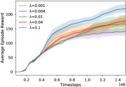
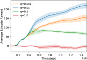
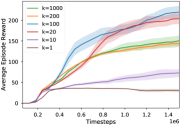
(a) $\lambda$ for entropy	(b) $\eta$ for dual	(c) $k$ for steps

Figure 1: The ablation study of the SBEED on Swimmer-v1. We varied $\lambda$, $\eta$, and $k$ to justify the effect of each component in the algorithm.

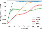
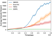
(a) Pendulum	(b) InvertedDoublePendulum

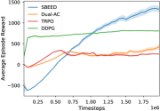
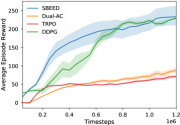
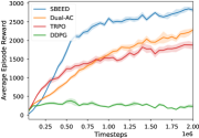
(c) HalfCheetah	(d) Swimmer	(e) Hopper

Figure 2: The results of SBEED against TRPO, Dual AC and DDPG. Each plot shows average reward during training across $5$ random runs, with $50\%$ confidence interval. The x-axis is the number of training iterations. SBEED achieves significant better performance than the competitors on all tasks.

The effect of smoothing.

We introduced the entropy regularization to avoid non-smoothness in Bellman error objective. However, as we discussed, it also introduces bias. We varied $\lambda$ and evaluated the performance of SBEED. The results in Figure 1(a) are as expected: there is indeed an intermediate value for $\lambda$ that gives the best bias/smoothness balance.

The effect of dual function.

One of the important components in our algorithm is the dual function, which cancels the variance. The effect of such cancellation is controlled by $\eta\in[0,1]$, and we expected an intermediate value gives the best performance. This is verified by the experiment of varying $\eta$, as shown in Figure 1(b).

The effect of multi-step.

SBEED can be easily extended to the multi-step version. However, increasing the length of steps will also increase the variance. We tested the performance of the algorithm with different $k$ values. The results shown in Figure 1(c) confirms that an intermediate value for $k$ yields the best result.

7.2 Comparison in Continuous Control Tasks

We tested SBEED across multiple continuous control tasks from the OpenAI Gym benchmark (Brockman et al., 2016) using the MuJoCo simulator (Todorov et al., 2012), including Pendulum-v0, InvertedDoublePendulum-v1, HalfCheetah-v1, Swimmer-v1, and Hopper-v1. For fairness, we follows the default setting of the MuJoCo simulator in each task in this section. These tasks have dynamics of different natures, so are helpful for evaluating the behavior of the proposed SBEED in different scenarios. We compared SBEED with several state-of-the-art algorithms, including two on-policy algorithms, trust region policy optimization (TRPO) (Schulman et al., 2015) dual actor-critic (Dual AC) (Dai et al., 2018), and one off-policy algorithm, deep deterministic policy gradient (DDPG) (Lillicrap et al., 2015). We did not include PCL (Nachum et al., 2017) as it is a special case of our algorithm by setting $\eta=0$, i.e., ignoring the updates for dual function. Since TRPO and Dual-AC are only applicable for on-policy setting, for fairness, we also conducted the comparison with these two algorithm in on-policy setting. Due to the space limitation, the results can be found in Appendix E.

We ran the algorithm with $5$ random seeds and reported the average rewards with 50% confidence intervals. The results are shown in Figure 2. We can see that our SBEED algorithm achieves significantly better performance than all other algorithms across the board. These results suggest that the SBEED can exploit the off-policy samples efficiently and stably, and achieve a good trade-off between bias and variance.

It should be emphasized that the stability of algorithm is an important issue in reinforcement learning. As we can see from the results, although DDPG can also exploit the off-policy sample, which promotes its efficiency in stable environments, e.g., HalfCheetah-v1 and Swimmer-v1, it may fail to learn in unstable environments, e.g., InvertedDoublePendulum-v1 and Hopper-v1, which was observed by Henderson et al. (2018) and Haarnoja et al. (2018). In contrast, SBEED is consistently reliable and effective in different tasks.

8 Conclusion

We provide a new optimization perspective of the Bellman equation, based on which we develop the new SBEED algorithm for policy optimization in reinforcement learning. The algorithm is provably convergent even when nonlinear function approximation is used on off-policy samples. We also provide PAC bound to characterize the sample complexity based on one single off-policy sample path collected by a fixed behavior policy. Empirical study shows the proposed algorithm achieves superior performance across the board, compared to state-of-the-art baselines on several MuJoCo control tasks.

Appendix

Appendix A Properties of Smoothed Bellman Operator

After applying the smoothing technique (Nesterov, 2005), we obtain a new Bellman operator, $\widetilde{\mathcal{T}}$, which is contractive. By such property, we can guarantee the uniqueness of the solution; a similar result is also presented in Fox et al. (2016); Asadi & Littman (2017).

Proposition 1 (Contraction) ${\mathcal{T}}_{\lambda}$ is a $\gamma$-contraction. Consequently, the corresponding smoothed Bellman equation (4), or equivalently (5), has a unique solution $V_{\lambda}^{*}$.

Proof  For any $V_{1},V_{2}:{\mathcal{S}}\to\mathbb{R}$, we have

$$\left\|\widetilde{\mathcal{T}}V_{1}-\widetilde{\mathcal{T}}V_{2}\right\|_{\infty}$$

$$= \left\|\max_{\pi}\left\{\left\langle\pi,R(s,a)+\gamma\mathbb{E}_{s^{\prime}|s,a}\left[V_{1}(s^{\prime})\right]\right\rangle+\lambda H(\pi)\right\}-\max_{\pi}\left\{\left\langle\pi,R(s,a)+\gamma\mathbb{E}_{s^{\prime}|s,a}\left[V_{2}(s^{\prime})\right]\right\rangle+\lambda H(\pi)\right\}\right\|_{\infty}$$

$$\leqslant \left\|\max_{\pi}\left\{\left\langle\pi,R(s,a)+\gamma\mathbb{E}_{s^{\prime}|s,a}\left[V_{1}(s^{\prime})\right]\right\rangle+\lambda H(\pi)-\left\langle\pi,R(s,a)+\gamma\mathbb{E}_{s^{\prime}|s,a}\left[V_{2}(s^{\prime})\right]\right\rangle-\lambda H(\pi)\right\}\right\|$$

$$\leqslant \left\|\max_{\pi}\left\langle\pi,\gamma\mathbb{E}_{s^{\prime}|s,a}\left[V_{1}(s^{\prime})-V_{2}(s^{\prime})\right]\right\rangle\right\|_{\infty}$$

$$\leqslant \gamma\left\|V_{1}-V_{2}\right\|_{\infty}\,.$$

${\mathcal{T}}_{\lambda}$ is therefore a $\gamma$-contraction and, by the Banach fixed point theorem, admits a unique fixed point.  

Moreover, we may characterize the bias introduced by the entropic smoothing, similar to the simulation lemma (see, e.g., Kearns & Singh (2002) and Strehl et al. (2009)):

Proposition 2 (Smoothing bias) Let $V^{*}$ and $V_{\lambda}^{*}$ be the fixed points of (2) and (4), respectively. It holds that

$$\left\|V^{*}-V_{\lambda}^{*}\right\|_{\infty}\leqslant\frac{\lambda H^{*}}{1-\gamma}.$$

As $\lambda\to 0$, $V_{\lambda}^{*}$ converges to $V^{*}$ pointwisely.

Proof  Using the triangle inequality and the contraction property of ${\mathcal{T}}_{\lambda}$, we have

$$\left\|V^{*}-V_{\lambda}^{*}\right\|_{\infty} = \left\|{\mathcal{T}}V^{*}-{\mathcal{T}}_{\lambda}V_{\lambda}^{*}\right\|_{\infty}$$

$$= \left\|V^{*}-{\mathcal{T}}_{\lambda}V^{*}+{\mathcal{T}}_{\lambda}V^{*}-{\mathcal{T}}_{\lambda}V_{\lambda}^{*}\right\|_{\infty}$$

$$\leqslant \left\|V^{*}-{\mathcal{T}}_{\lambda}V^{*}\right\|_{\infty}+\left\|{\mathcal{T}}_{\lambda}V^{*}-{\mathcal{T}}_{\lambda}V_{\lambda}^{*}\right\|_{\infty}$$

$$\leqslant \lambda H^{*}+\gamma\left\|V^{*}-V_{\lambda}^{*}\right\|_{\infty}\,,$$

which immediately implies the desired bound.  

The smoothed Bellman equation involves a $\log$-sum-$\exp$ operator to approximate the $\max$-operator, which increases the nonlinearity of the equation. We further characterize the solution of the smoothed Bellman equation, by the temporal consistency conditions.

Theorem 3 (Temporal consistency) Assume $\lambda>0$. Let $V_{\lambda}^{*}$ be the fixed point of (4) and $\pi_{\lambda}^{*}$ the corresponding policy that attains the maximum on the RHS of (4). Then, $(V,\pi)=(V_{\lambda}^{*},\pi_{\lambda}^{*})$ if and only if $(V,\pi)$ satisfies the following equality for all $(s,a)\in{\mathcal{S}}\times\mathcal{A}$:

$$V(s)=R(s,a)+\gamma\mathbb{E}_{s^{\prime}|s,a}\left[V(s^{\prime})\right]-\lambda\log\pi(a|s)\,.$$ (7)

Proof  The proof has two parts.
(Necessity) We need to show $(V_{\lambda}^{*},\pi_{\lambda}^{*})$ is a solution to (6). Simple calculations give the closed form of $\pi_{\lambda}^{*}$:

$$\pi_{\lambda}^{*}(a|s)=Z(s)^{-1}\exp\left(\frac{R(s,a)+\gamma\mathbb{E}_{s^{\prime}|s,a}\left[V_{\lambda}^{*}(s^{\prime})\right]}{\lambda}\right)\,,$$

where $Z(s):=\sum_{a\in\mathcal{A}}\exp\left(\frac{R(s,a)+\gamma\mathbb{E}_{s^{\prime}|s,a}\left[V_{\lambda}^{*}(s^{\prime})\right]}{\lambda}\right)$ is a state-dependent normalization constant. Therefore, for any $a\in\mathcal{A}$,

$$R(s,a)+\gamma\mathbb{E}_{s^{\prime}|s,a}\left[V_{\lambda}^{*}(s^{\prime})\right]-\lambda\log\pi_{\lambda}^{*}(a|s)$$

$$= R(s,a)+\gamma\mathbb{E}_{s^{\prime}|s,a}\left[V_{\lambda}^{*}(s^{\prime})\right]-\lambda\left(\frac{R(s,a)+\gamma\mathbb{E}_{s^{\prime}|s,a}\left[V_{\lambda}^{*}(s^{\prime})\right]}{\lambda}-\log Z(s)\right)$$

$$= \lambda\log Z(s)\,\,=\,\,V_{\lambda}^{*}(s)\,,$$

where the last step is from (5). Therefore, $(V_{\lambda}^{*},\pi_{\lambda}^{*})$ satisfies (6).

(Sufficiency) Assume $\bar{V}$ and $\bar{\pi}$ satisfies (6), then we have for all $(s,a)\in{\mathcal{S}}\times\mathcal{A}$ that

$$\bar{V}(s) = R(s,a)+\gamma\mathbb{E}_{s^{\prime}|s,a}\left[\bar{V}(s^{\prime})\right]-\lambda\log\bar{\pi}(a|s)$$

$$\pi(a|s) = \exp\left(\frac{R(s,a)+\gamma\mathbb{E}_{s^{\prime}|s,a}\left[\bar{V}(s^{\prime})\right]-\bar{V}(s)}{\lambda}\right)\,.$$

Recall $\pi(\cdot|s)\in\mathcal{P}$, we have

$$\sum_{a\in\mathcal{A}}\exp\left(\frac{R(s,a)+\gamma\mathbb{E}_{s^{\prime}|s,a}\left[\bar{V}(s^{\prime})\right]-\bar{V}(s)}{\lambda}\right)=1$$

$$\Rightarrow \sum_{a\in\mathcal{A}}\exp\left(\frac{R(s,a)+\gamma\mathbb{E}_{s^{\prime}|s,a}\left[\bar{V}(s^{\prime})\right]}{\lambda}\right)=\exp\left(\frac{\bar{V}(s)}{\lambda}\right)$$

$$\Rightarrow \bar{V}(s)=\lambda\log\left(\sum_{a\in\mathcal{A}}\exp\left(\frac{R(s,a)+\gamma\mathbb{E}_{s^{\prime}|s,a}\left[\bar{V}(s^{\prime})\right]}{\lambda}\right)\right)={\mathcal{T}}_{\lambda}\bar{V}(s)\,.$$

The last equation holds for all $s\in{\mathcal{S}}$, so $\bar{V}$ is a fixed point of ${\mathcal{T}}$. It then follows from Proposition 1 that $\bar{V}=V_{\lambda}^{*}$. Finally, $\bar{\pi}=\pi_{\lambda}^{*}$ due to strong concavity of the entropy function  

The same conditions have been re-discovered several times, e.g., (Rawlik et al., 2012; Nachum et al., 2017), from a completely different point of views.

Appendix B Variance Cancellation via the Saddle Point Formulation

The second term in the saddle point formulation (9) will cancel the variance $\mathbb{V}_{s,a,s^{\prime}}\left[\gamma V(s^{\prime})\right]$. Formally,

Proposition 8

Given any fixed $(V,\pi)$, we have

$$\max_{\rho\in\mathcal{F}\left({\mathcal{S}}\times\mathcal{A}\right)}-\mathbb{E}_{s,a,s^{\prime}}\left[\left({R(s,a)+\gamma{V(s^{\prime})-\lambda\log\pi(a|s)}}-\rho(s,a)\right)^{2}\right]=-\gamma^{2}\mathbb{E}_{s,a}\left[\mathbb{V}_{s^{\prime}|s,a}\left[V(s^{\prime})\right]\right].$$ (11)

Proof  Recall from (9) that $\delta(s,a,s^{\prime})=R(s,a)+\gamma{V(s^{\prime})-\lambda\log\pi(a|s)}$. Then,

$$\max_{\rho}\,\,-\mathbb{E}_{s,a,s^{\prime}}\left[\left({R(s,a)+\gamma{V(s^{\prime})-\lambda\log\pi(a|s)}}-\rho(s,a)\right)^{2}\right]$$

$$= -\min_{\rho}\,\,\mathbb{E}_{s,a}\left[\mathbb{E}_{s^{\prime}|s,a}\left[\left(\delta(s,a,s^{\prime})-\rho(s,a)\right)^{2}\right]\right]\,.$$

Clearly, the minimizing function $\rho^{*}$ may be determined for each $(s,a)$ entry separately. Fix any $(s,a)\in{\mathcal{S}}\times\mathcal{A}$, and define a function on $\mathbb{R}$ as $q(x):=\mathbb{E}_{s^{\prime}|s,a}\left[\left(\delta(s,a,s^{\prime})-x\right)^{2}\right]$. Obviously, this convex function is minimized at the stationary point $x^{*}=\mathbb{E}_{s^{\prime}|s,a}\left[\delta(s,a,s^{\prime})\right]$. We therefore have $\rho^{*}(s,a)=\mathbb{E}_{s^{\prime}|s,a}\left[\delta(s,a,s^{\prime})\right]$ for all $(s,a)$, so

$$\min_{\rho}\,\,\mathbb{E}_{s,a}\left[\mathbb{E}_{s^{\prime}|s,a}\left[\left(\delta(s,a,s^{\prime})-\rho(s,a)\right)^{2}\right]\right]$$

$$= \mathbb{E}_{s,a}\left[\mathbb{E}_{s^{\prime}|s,a}\left[\left(\delta(s,a,s^{\prime})-\mathbb{E}_{s^{\prime}|s,a}\left[\delta(s,a,s^{\prime})\right]\right)^{2}\right]\right]$$

$$= \mathbb{E}_{s,a}\left[\mathbb{V}_{s^{\prime}|s,a}\left[\delta(s,a,s^{\prime})\right]\right]$$

$$= \mathbb{E}_{s,a}\left[\mathbb{V}_{s^{\prime}|s,a}\left[\gamma V(s^{\prime})\right]\right]\,\,=\,\,\gamma^{2}\mathbb{E}_{s,a}\left[\mathbb{V}_{s^{\prime}|s,a}\left[V(s^{\prime})\right]\right]\,,$$

where the second last step is due to the fact that, conditioned on $s$ and $a$, the only random variable in $\delta(s,a,s^{\prime})$ is $V(s^{\prime})$.  

Appendix C Details of SBEED

In this section, we provide further details of the SBEED algorithms, including its gradient derivation and multi-step/eligibility-trace extension.

C.1 Unbiasedness of Gradient Estimator

In this subsection, we compute the gradient with respect to the primal variables. Let $(w_{V},w_{\pi})$ be the parameters of the primal $(V,\pi)$, and $w_{\rho}$ the parameters of the dual $\rho$. Abusing notation a little bit, we now write the objective function $L_{\eta}(V,\pi;\rho)$ as $L_{\eta}(w_{V},w_{\pi};w_{\rho})$. Recall the quantity $\delta(s,a,s^{\prime})$ from (9).

Theorem 4 (Gradient derivation) Define $\bar{\ell}_{\eta}(w_{V},w_{\pi}):=L_{\eta}(w_{V},w_{\pi};w_{\rho}^{*})$, where $w_{\rho}^{*}=\arg\max_{w_{\rho}}L_{\eta}(w_{V},w_{\pi};w_{\rho})$. Let $\delta_{s,a,s^{\prime}}$ be a shorthand for $\delta(s,a,s^{\prime})$, and $\hat{\rho}$ be dual parameterized by $w_{\rho}^{*}$. Then,

$$\nabla_{w_{V}}\bar{\ell}_{\eta}= 2\mathbb{E}_{s,a,s^{\prime}}\left[\left(\delta_{s,a,s^{\prime}}-V(s)\right)\left(\gamma{\nabla_{w_{V}}V(s^{\prime})}-\nabla_{w_{V}}V(s)\right)\right]-2\eta\gamma\mathbb{E}_{s,a,s^{\prime}}\left[\left(\delta_{s,a,s^{\prime}}-\hat{\rho}(s,a)\right)\nabla_{w_{V}}V(s^{\prime})\right]\,,$$

$$\nabla_{w_{\pi}}\bar{\ell}_{\eta}= -2\lambda\mathbb{E}_{s,a,s^{\prime}}\big{[}\left((1-\eta)\delta_{s,a,s^{\prime}}+\eta\hat{\rho}(s,a)-V(s)\right)\cdot\nabla_{w_{\pi}}\log\pi(a|s)\big{]}\,.$$

Proof  First, note that $w_{\rho}^{*}$ is an implicit function of $(w_{V},w_{\pi})$. Therefore, we must use the chain rule to compute the gradient:

$$\nabla_{w_{V}}\bar{\ell}_{\eta} = 2\mathbb{E}_{s,a,s^{\prime}}\left[\left(\delta_{s,a,s^{\prime}}-V(s;w_{V})\right)\left(\gamma{\nabla_{w_{V}}V(s^{\prime};w_{V})}-\nabla_{w_{V}}V(s;w_{V})\right)\right]$$

$$-2\eta\gamma\mathbb{E}_{s,a,s^{\prime}}\left[\left(\delta_{s,a,s^{\prime}}-\rho(s,a;w_{\rho}^{*})\right)\nabla_{w_{V}}V(s^{\prime};w_{V})\right]$$

$$+2\eta\gamma\mathbb{E}_{s,a,s^{\prime}}\left[\left(\delta_{s,a,s^{\prime}}-\rho(s,a;w_{\rho}^{*})\right)\nabla_{w_{V}}\rho(s,a;w_{\rho}^{*})\right]\,.$$

We next show that the last term is zero:

$$\mathbb{E}_{s,a,s^{\prime}}\left[\left(\delta_{s,a,s^{\prime}}-\rho(s,a;w_{\rho}^{*})\right)\nabla_{w_{V}}\rho(s,a;w_{\rho}^{*})\right]$$

$$= \mathbb{E}_{s,a,s^{\prime}}\left[\left(\delta_{s,a,s^{\prime}}-\rho(s,a;w_{\rho}^{*})\right)\cdot\nabla_{w_{V}}w_{\rho}^{*}\cdot\nabla_{w_{\rho}}\rho(s,a;w_{\rho}^{*})\right]$$

$$= \nabla_{w_{V}}w_{\rho}^{*}\cdot\mathbb{E}_{s,a,s^{\prime}}\left[\left(\delta_{s,a,s^{\prime}}-\rho(s,a;w_{\rho}^{*})\right)\cdot\nabla_{w_{\rho}}\rho(s,a;w_{\rho}^{*})\right]$$

$$= \nabla_{w_{V}}w_{\rho}^{*}\cdot\mathbf{0}\,\,=\,\,\mathbf{0}\,,$$

where the first step is the chain rule; the second is due to the fact that $\nabla_{w_{V}}w_{\rho}^{*}$ is not a function of $(s,a,s^{\prime})$, so can be moved outside of the expectation; the third step is due to the optimality of $w_{\rho}^{*}$. The gradient w.r.t. $w_{V}$ is thus derived. The case for $w_{\pi}$ is similar.  

C.2 Multi-step Extension

One way to interpret the smoothed Bellman equation (4) is to treat each $\pi(\cdot|s)$ as a (mixture) action; in other words, the action space is now the simplex $\mathcal{P}_{\mathcal{A}}$. With this interpretation, the introduced entropy regularization may be viewed as a shaping reward: given a mixture action $\pi(\cdot|s)$, its immediate reward is given by

$$\tilde{R}(s,\pi(\cdot|s)):=\mathbb{E}_{a\sim\pi(\cdot|s)}\left[R(s,a)\right]+\lambda H(\pi,s)\,.$$

The transition probabilities can also be adapted accordingly as follows

$$\tilde{P}(s^{\prime}|s,\pi(\cdot|s)):=\mathbb{E}_{a\in\pi(\cdot|s)}\left[P(s^{\prime}|s,a)\right]\,.$$

It can be verified that the above constructions induce a well-defined MDP $\tilde{M}=\langle{\mathcal{S}},\mathcal{P}_{\mathcal{A}},\tilde{P},\tilde{R},\gamma\rangle$, whose standard Bellman equation is exactly (4).

With this interpretation, the proposed framework and algorithm can be easily applied to multi-step and eligibility-traces extensions. Specifically, one can show that $(V_{\lambda}^{*},\pi_{\lambda}^{*})$ is the unique solution that satisfies the multi-step expansion of (6): for any $k\geqslant 1$ and any $(s_{0},a_{0},a_{1},\ldots,a_{k-1})\in{\mathcal{S}}\times\mathcal{A}^{k}$,

$$V(s_{0})=\sum_{t=0}^{k-1}\gamma^{t}\mathbb{E}_{s_{t}|s_{0},a_{0:t-1}}\left[R(s_{t},a_{t})-\lambda\log\pi(a_{t}|s_{t})\right]+\gamma^{k}\mathbb{E}_{s_{k}|s_{0},a_{0:k-1}}\left[V(s_{k})\right]\,.$$ (12)

Clearly, when $k=1$ (the single-step bootstrapping case), the above equation reduces to (6).

The $k$-step extension of objective function (7) now becomes

$$\min_{V,\pi}\mathbb{E}_{s_{0},a_{0:k-1}}\left[\left(\sum_{t=0}^{k-1}\gamma^{t}\mathbb{E}_{s_{t}|s_{0},a_{0:t-1}}\left[R(s_{t},a_{t})-\lambda\log\pi(a_{t}|s_{t})\right]+\gamma^{k}\mathbb{E}_{s_{k}|s_{0},a_{0:k-1}}\left[V(s_{k})\right]-V(s_{0})\right)^{2}\right].$$

Applying the Legendre-Fenchel transformation and the interchangeability principle, we arrive at the following multi-step primal-dual optimization problem:

$$\min_{V,\pi}\max_{\nu} \mathbb{E}_{s_{0},a_{0:t-1}}\bigg{[}\nu(s_{0},a_{0:t-1})\bigg{(}\sum_{t=0}^{k-1}\gamma^{t}\mathbb{E}_{s_{t}|s_{0},a_{0:k-1}}\left[R(s_{t},a_{t})-\lambda\log\pi(a_{t}|s_{t})\right]$$

$$+\gamma^{k}\mathbb{E}_{s_{k}|s_{0},a_{0:k-1}}\left[V(s_{k})\right]-V(s_{0})\bigg{)}\bigg{]}-\frac{1}{2}\mathbb{E}_{s_{0},a_{0:k-1}}\left[\nu(s_{0},a_{0:k-1})^{2}\right]$$

$$=\min_{V,\pi}\max_{\nu} \mathbb{E}_{s_{0:k},a_{0:k-1}}\bigg{[}\nu(s_{0},a_{0:k-1})\bigg{(}\sum_{t=0}^{k-1}\gamma^{t}\left({R(s_{t},a_{t})-\lambda\log\pi(a_{t}|s_{t})}\right)$$

$$+\gamma^{k}{V(s_{k})}-V(s_{0})\bigg{)}\bigg{]}-\frac{1}{2}\mathbb{E}_{s_{0},a_{0:k-1}}\left[\nu(s_{0},a_{0:k-1})^{2}\right].$$

Similar to the single-step case, defining

$$\delta(s_{0:k},a_{0:k-1}):=\sum_{t=0}^{k-1}\gamma^{t}\left(R(s_{t},a_{t})-\lambda\log\pi(a_{t}|s_{t})\right)+\gamma^{k}{V(s_{k})}\,.$$

and using the substitution $\rho(s_{0},a_{0:k-1})=\nu(s_{0},a_{0:k-1})+V(s_{0})$, we reach the following saddle-point formulation:

$$\min_{V,\pi}\max_{\rho}L(V,\pi;\rho):=\mathbb{E}_{s_{0:k},a_{0:k-1}}\left[\left(\delta(s_{0:k},a_{0:k-1})-V(s_{0})\right)^{2}-\eta\left({\delta(s_{0:k},a_{0:k-1})}-\rho(s_{0},a_{0:k-1})\right)^{2}\right]$$ (13)

where the dual function now is $\rho(s_{0},a_{0:k-1})$, a function on ${\mathcal{S}}\times\mathcal{A}^{k}$, and $\eta\geqslant 0$ is again a parameter used to balance between bias and variance. It is straightforward to generalize Theorem 4 to the multi-step setting, and to adapt SBEED accordingly,

C.3 Eligibility-trace Extension

Eligibility traces can be viewed as an approach to aggregating multi-step bootstraps for $k\in\{1,2,\cdots\}$; see Sutton & Barto (1998) for more discussions. The same can be applied to the multi-step consistency condition (12), using an exponential weighting parameterized by $\zeta\in[0,1)$. Specifically, for all $(s_{0},a_{0:k-1})\in{\mathcal{S}}\times\mathcal{A}^{k}$, we have

$$V(s_{0})=(1-\zeta)\sum_{k=1}^{\infty}\zeta^{k-1}\left(\sum_{t=0}^{k-1}\gamma^{t}\mathbb{E}_{s_{t}|s_{0},a_{0:k-1}}\left[R(s_{t},a_{t})-\lambda\log\pi(a_{t}|s_{t})\right]+\gamma^{k}\mathbb{E}_{s_{k}|s_{0},a_{0:k-1}}\left[V(s_{k})\right]\right)\,.$$ (14)

Then, following similar steps as in the previous subsection, we reach the following saddle-point optimization:

$$\min_{V,\pi}\max_{\rho} \mathbb{E}_{s_{0:\infty},a_{0:\infty}}\left[\left((1-\zeta)\sum_{k=1}^{\infty}\zeta^{k-1}\delta(s_{0:k},a_{0:k-1})-V(s_{0})\right)^{2}\right]$$ (15)

$$-\eta\,\mathbb{E}_{s_{0:\infty},a_{0:\infty}}\left[\left({(1-\zeta)\sum_{k=1}^{\infty}\zeta^{k-1}\delta(s_{0:k},a_{0:k-1})}-\rho(s_{0},a_{0:\infty})\right)^{2}\right]\,.$$

In practice, $\rho(s_{0},a_{0:\infty})$ can be parametrized by neural networks with finite length of actions as input as an approximation.

Appendix D Proof Details of the Theoretical Analysis

In this section, we provide the details of the analysis in Theorems 6 and 7. We start with the boundedness of $V^{*}$ and $V_{\lambda}^{*}$ under Assumption 1. Given any measure on the state space ${\mathcal{S}}$,

$$\left\|V^{*}\right\|_{\mu}\leqslant\left\|V^{*}\right\|_{\infty}\leqslant(1+\gamma+\gamma^{2}+\cdots)C_{R}=C_{V}:=\frac{C_{R}}{1-\gamma}\,.$$

A similar argument may be used on $V_{\lambda}^{*}$ to get

$$\left\|V_{\lambda}^{*}\right\|_{\mu}\leqslant\frac{C_{R}+H^{*}}{1-\gamma}\,.$$

It should be emphasized that although Assumption 1 ensures boundedness of $V^{*}$ and $\log\pi^{*}(a|s)$, it does not imply the continuity and smoothness. In fact, as we will see later, $\lambda$ controls the trade-off between approximation error (due to parameterization) and bias (due to smoothing) in the solution of the smoothed Bellman equation.

D.1 Error Decomposition

Recall that

• $(V^{*},\pi^{*})$ corresponds to the optimal value function and optimal policy to the original Bellman equation, namely, they are solutions to the optimization problem (3);

• $(V_{\lambda}^{*},\pi_{\lambda}^{*})$ corresponds to the optimal value function and optimal policy to the smoothed Bellman equation, namely, they are solutions to the optimization problem (7) with objective $\ell(V,\pi)$;

• $(V^{*}_{w},\pi^{*}_{w})$ correponds to the optimal solution to the optimization problem (7) under nonlinear function approximation, with objective $\ell_{w}(V_{w},\pi_{w})$;

• $(\widehat{V}^{*}_{w},\widehat{\pi}^{*}_{w})$ stands for the optimal solution to the finite sample approximation of (7) under nonlinear function approximation, with objective $\widehat{\ell}_{T}(V_{w},\pi_{w})$.

Hence, we can decompose the error between $(\widehat{V}^{*}_{w},\widehat{\pi}^{*}_{w})$ and $(V_{\lambda}^{*},\pi_{\lambda}^{*})$ under the $\left\|\cdot\right\|_{\mu\pi_{b}}$ norm.

$$\left\|\widehat{V}_{w}^{*}-V^{*}\right\|_{\mu\pi_{b}}^{2} \leqslant 2\left\|\widehat{V}_{w}^{*}-V_{\lambda}^{*}\right\|_{\mu\pi_{b}}^{2}+2\left\|V_{\lambda}^{*}-V^{*}\right\|^{2}_{\mu\pi_{b}}.$$ (16)

We first look at the second term from smoothing error, which can be similarly bounded, as shown in Proposition 2.

Lemma 9 (Smoothing bias)

$\left\|V_{\lambda}^{*}-V^{*}\right\|^{2}_{\mu\pi_{b}}\leqslant(2\gamma^{2}+2)\left(\frac{\gamma\lambda}{1-\gamma}\max_{\pi\in\mathcal{P}}H(\pi)\right)^{2}$.

Proof  For $\left\|V_{\lambda}^{*}-V^{*}\right\|^{2}_{\mu\pi_{b}}$, we have

$$\left\|V_{\lambda}^{*}-V^{*}\right\|^{2}_{\mu\pi_{b}} = \int\left(\gamma\mathbb{E}_{s^{\prime}|s,a}\left[V^{*}(s^{\prime})-V_{\lambda}^{*}(s^{\prime})\right]-\left(V^{*}(s)-V_{\lambda}^{*}(s)\right)\right)^{2}\mu(s)\pi_{b}(a|s)dsda$$

$$\leqslant 2\gamma^{2}\left\|\mathbb{E}_{s^{\prime}|s,a}\left[V^{*}(s^{\prime})-V_{\lambda}^{*}(s^{\prime})\right]\right\|_{\infty}^{2}+2\left\|V^{*}(s)-V_{\lambda}^{*}(s)\right\|_{\infty}$$

$$\leqslant (2\gamma^{2}+2)\left(\frac{\gamma\lambda}{1-\gamma}\max_{\pi\in\mathcal{P}}H(\pi)\right)^{2},$$

where the final inequality is because Lemma 2.  

We now look at the first term and show that

Lemma 10

$$\left\|\widehat{V}_{w}^{*}-V_{\lambda}^{*}\right\|^{2}_{\mu\pi_{b}} \leqslant 2\left(\ell(\widehat{V}_{w}^{*},\widehat{\pi}_{w}^{*})-\ell(V_{\lambda}^{*},\pi_{\lambda}^{*})\right)+4\lambda^{2}\left\|\log{\widehat{\pi}_{w}^{*}(a|s)}-\log{\hat{\pi}_{w}^{*}(a|s)}\right\|_{2}^{2}$$

$$+4\lambda^{2}\left\|\log{\pi_{w}^{*}(a|s)}-\log{\pi_{\lambda}^{*}(a|s)}\right\|_{2}^{2}.$$

Proof  Specifically, due to the strongly convexity of square function, we have

$$\ell(\widehat{V}_{w}^{*},\widehat{\pi}_{w}^{*})-\ell(V_{\lambda}^{*},\pi_{\lambda}^{*}) = 2\mathbb{E}\left[\bar{\Delta}_{V_{\lambda}^{*},\pi_{\lambda}^{*}}(s,a)\left(\bar{\Delta}_{\widehat{V}_{w}^{*},\widehat{\pi}_{w}^{*}}(s,a)-\bar{\Delta}_{V_{\lambda}^{*},\pi_{\lambda}^{*}}(s,a)\right)\right]$$

$$+ \mathbb{E}_{\mu\pi_{b}}\left[\left(\bar{\Delta}_{\widehat{V}_{w}^{*},\widehat{\pi}_{w}^{*}}(s,a)-\bar{\Delta}_{V_{\lambda}^{*},\pi_{\lambda}^{*}}(s,a)\right)^{2}\right]$$

$$\geqslant \int\left(\bar{\Delta}_{\widehat{V}_{w}^{*},\widehat{\pi}_{w}^{*}}(s,a)-\bar{\Delta}_{V_{\lambda}^{*},\pi_{\lambda}^{*}}(s,a)\right)^{2}\mu(s)\pi_{b}(a|s)dsda$$

$$:= \left\|\bar{\Delta}_{\widehat{V}_{w}^{*},\widehat{\pi}_{w}^{*}}(s,a)-\bar{\Delta}_{V_{\lambda}^{*},\pi_{\lambda}^{*}}(s,a)\right\|_{2}^{2},$$

where $\Delta(s,a,s^{\prime})={R(s,a)+\gamma{V(s^{\prime})-\lambda\log\pi(a|s)}-V(s)}$ and the second inequality is because the optimality of $V_{\lambda}^{*}$ and $\pi_{\lambda}^{*}$. Therefore, we have

$$\sqrt{\ell(\widehat{V}_{w}^{*},\widehat{\pi}_{w}^{*})-\ell(V_{\lambda}^{*},\pi_{\lambda}^{*})}\geqslant\left\|\bar{\Delta}_{\widehat{V}_{w}^{*},\widehat{\pi}_{w}^{*}}(s,a)-\bar{\Delta}_{V_{\lambda}^{*},\pi_{\lambda}^{*}}(s,a)\right\|_{2}$$

$$\geqslant \left|\left\|\gamma\mathbb{E}_{s^{\prime}|s,a}\left[\widehat{V}_{w}^{*}(s^{\prime})-V_{\lambda}^{*}(s^{\prime})\right]-\left(\widehat{V}_{w}^{*}(s)-V_{\lambda}^{*}(s)\right)\right\|_{2}-\lambda\left\|\log{\widehat{\pi}_{w}^{*}(a|s)}-\log{\pi_{\lambda}^{*}(a|s)}\right\|_{2}\right|$$

$$= \left|\left\|\widehat{V}_{w}^{*}-V_{\lambda}^{*}\right\|_{\mu\pi_{b}}-\lambda\left\|\log{\widehat{\pi}_{w}^{*}(a|s)}-\log{\pi_{\lambda}^{*}(a|s)}\right\|_{2}\right|$$

which implies

$$\left\|\widehat{V}_{w}^{*}-V_{\lambda}^{*}\right\|^{2}_{\mu\pi_{b}} \leqslant 2\left(\ell(\widehat{V}_{w}^{*},\widehat{\pi}_{w}^{*})-\ell(V_{\lambda}^{*},\pi_{\lambda}^{*})\right)+2\lambda^{2}\left\|\log{\widehat{\pi}_{w}^{*}(a|s)}-\log{\pi_{\lambda}^{*}(a|s)}\right\|_{2}^{2}$$

$$\leqslant 2\left(\ell(\widehat{V}_{w}^{*},\widehat{\pi}_{w}^{*})-\ell(V_{\lambda}^{*},\pi_{\lambda}^{*})\right)+4\lambda^{2}\left\|\log{\widehat{\pi}_{w}^{*}(a|s)}-\log{\pi_{w}^{*}(a|s)}\right\|_{2}^{2}$$

$$+4\lambda^{2}\left\|\log{\pi_{w}^{*}(a|s)}-\log{\pi_{\lambda}^{*}(a|s)}\right\|_{2}^{2}.$$

 

In regular MDP with Assumption 1, with appropriate $C$, such constraint does not introduce any loss. We denote the family of value functions and policies by parametrization as $\mathcal{V}_{w},\,\mathcal{P}_{w}$, respectively. Then, for $V$ and $\log\pi$ uniformly bounded by $C_{\infty}=\max\left\{\frac{C_{R}}{1-\gamma},C_{\pi}\right\}$ and the square loss is uniformly $K$-Lipschitz continuous, by proposition in Dai et al. (2016), we have

Corollary 11

$\ell(V,\pi)-\ell_{w}(V,\pi)\leqslant(K+C_{\infty})\epsilon_{\text{app}}^{\nu}$ where $\epsilon_{\text{app}}=\sup_{\nu\in\mathcal{C}}\inf_{h\in\mathcal{H}}\left\|\nu-h\right\|_{\infty}$ with $\mathcal{C}$ denoting the Lipschitz continuous function space and $\mathcal{H}$ denoting the hypothesis space.

Proof  Denote the $\phi(V,\pi,\nu):=\mathbb{E}_{s,a,s^{\prime}}\left[\nu(s,a)\left(R(s,a)+\gamma{V(s^{\prime})-\lambda\log\pi(a|s)}-V(s)\right)\right]-\frac{1}{2}\mathbb{E}_{s,a,s^{\prime}}\left[\nu^{2}(s,a)\right]$, we have $\phi(V,\pi,\nu)$ is $(K+C_{\infty})$-Lipschitz continuous w.r.t. $\left\|\cdot\right\|_{\infty}$. Denote $\nu_{V,\pi}^{*}=\mathop{\mathrm{argmax}}_{\nu}\phi(V,\pi,\nu)$, $\nu_{V,\pi}^{\mathcal{H}}=\mathop{\mathrm{argmax}}_{\nu\in\mathcal{H}}\phi(V,\pi,\nu)$, and $\hat{\nu}_{V,\pi}=\min_{\nu\in\mathcal{H}}\left\|\nu-\nu_{V,\pi}^{*}\right\|_{\infty}$

$$\ell(V,\pi)-\ell_{w}(V,\pi) = \phi(V,\pi,\nu_{V,\pi}^{*})-\phi(V,\pi,\nu_{V,\pi}^{\mathcal{H}})$$

$$\leqslant \phi(V,\pi,\nu_{V,\pi}^{*})-\phi(V,\pi,\hat{\nu}_{V,\pi})\leqslant(K+C_{\infty})\epsilon_{\text{app}}^{\nu}.$$

 

For the third term in Lemma 10, we have

$$\lambda\left\|\log{\pi_{w}^{*}(a|s)}-\log{\pi_{\lambda}^{*}(a|s)}\right\|^{2}_{2} \leqslant {\ell\left(V,\pi_{w}^{*}\right)-\ell\left(V,\pi_{\lambda}^{*}\right)}$$

$$= \ell_{w}\left(V,\pi_{w}^{*}\right)-\ell_{w}\left(V,\pi_{\lambda}^{*}\right)+\left(\ell\left(V,\pi_{w}^{*}\right)-\ell_{w}\left(V,\pi_{w}^{*}\right)\right)-\left(\ell\left(V,\pi_{\lambda}^{*}\right)-\ell_{w}\left(V,\pi_{\lambda}^{*}\right)\right)$$

$$\leqslant C_{\nu}\inf_{\pi_{w}}\left\|\lambda\log\pi_{w}-\lambda\log\pi_{\lambda}^{*}\right\|_{\infty}+2(K+C_{\infty})\epsilon_{\text{app}}^{\nu}$$

$$\leqslant C_{\nu}\epsilon_{\text{app}}^{\pi}(\lambda)+2(K+C_{\infty})\epsilon_{\text{app}}^{\nu}$$

where $C_{\nu}=\max_{\nu\in\mathcal{H}_{w}}\left\|\nu\right\|_{2}$. The first inequality comes from the strongly convexity of $\ell\left(V,\pi\right)$ w.r.t. $\lambda\log\pi$, the second inequality comes from Section 5 in Bach (2014) and Corollary 11 with $\epsilon_{\text{app}}^{\pi}(\lambda):=\sup_{\pi\in\mathcal{P}_{\lambda}}\inf_{\pi_{w}\in\mathcal{P}_{w}}\left\|\lambda\log\pi_{w}-\lambda\log\pi\right\|_{\infty}$ with

$$\mathcal{P}_{\lambda}:=\left\{\pi\in\mathcal{P},\pi(a|s)=\exp\left(\frac{Q(s,a)-\mathcal{L}(Q)}{\lambda}\right),\left\|Q\right\|_{2}\leqslant C_{V}\right\}.$$

Based on the derivation of $\mathcal{P}_{\lambda}$, with continuous $\mathcal{A}$, it can be seen that as $\lambda\rightarrow 0$,

$$\mathcal{P}_{0}=\left\{\pi\in\mathcal{P},\pi(a|s)=\delta_{a_{\max}(s)}(a)\right\},$$

which results $\epsilon_{\text{app}}^{\pi}(\lambda)\rightarrow\infty$, and as $\lambda$ increasing as finite, the policy becomes smoother, resulting smaller approximate error in general. With discrete $\mathcal{A}$, although the $\epsilon_{\text{app}}^{\pi}(0)$ is bounded, the approximate error still decreases as $\lambda$ increases. The similar correspondence also applies to $\epsilon_{\text{app}}^{V}(\lambda)$. The concrete correspondence between $\lambda$ and $\epsilon_{\text{app}}(\lambda)$ depends on the specific form of the function approximators, which is an open problem and out of the scope of this paper.

For the second term in 10,

$$\lambda\left\|\log{\widehat{\pi}_{w}^{*}(a|s)}-\log{\pi_{w}^{*}(a|s)}\right\|_{2}\leqslant\lambda\left\|\log{\widehat{\pi}_{w}^{*}(a|s)}\right\|_{2}+\lambda\left\|\log{\pi_{w}^{*}(a|s)}\right\|_{2}\leqslant 2\lambda C_{\pi}.$$ (18)

For the first term, we have

$$\ell(\widehat{V}_{w}^{*},\widehat{\pi}_{w}^{*})-\ell(V_{\lambda}^{*},\pi_{\lambda}^{*})$$

$$= \ell(\widehat{V}_{w}^{*},\widehat{\pi}_{w}^{*})-\ell_{w}(\widehat{V}_{w}^{*},\widehat{\pi}_{w}^{*})+\ell_{w}(\widehat{V}_{w}^{*},\widehat{\pi}_{w}^{*})-\ell_{w}(V_{\lambda}^{*},\pi_{\lambda}^{*})+\ell_{w}(V_{\lambda}^{*},\pi_{\lambda}^{*})-\ell(V_{\lambda}^{*},\pi_{\lambda}^{*})$$

$$\leqslant 2(K+C_{\infty})\epsilon_{\text{app}}^{\nu}+\ell_{w}(\widehat{V}_{w}^{*},\widehat{\pi}_{w}^{*})-\ell_{w}(V_{\lambda}^{*},\pi_{\lambda}^{*})$$

$$= 2(K+C_{\infty})\epsilon_{\text{app}}^{\nu}+\ell_{w}(\widehat{V}_{w}^{*},\widehat{\pi}_{w}^{*})-\ell_{w}(V_{w}^{*},\pi_{w}^{*})+{\ell_{w}(V_{w}^{*},\pi_{w}^{*})-\ell_{w}(V_{\lambda}^{*},\pi_{\lambda}^{*})}$$

$$\leqslant 2(K+C_{\infty})\epsilon_{\text{app}}^{\nu}+C_{\nu}\left((1+\gamma)\epsilon_{\text{app}}^{V}(\lambda)+\epsilon_{\text{app}}^{\pi}(\lambda)\right)+\ell_{w}(\widehat{V}_{w}^{*},\widehat{\pi}_{w}^{*})-\ell_{w}(V_{w}^{*},\pi_{w}^{*}).$$

The last inequality is because

$$\ell_{w}(V_{w}^{*},\pi_{w}^{*})-\ell_{w}(V_{\lambda}^{*},\pi_{\lambda}^{*}) = \inf_{V_{w},\pi_{w}}\ell_{w}(V_{w},\pi_{w})-\ell_{w}(V_{\lambda}^{*},\pi_{\lambda}^{*})$$

$$\leqslant C_{\nu}\inf_{V_{w},\pi_{w}}\left(\left(1+\gamma\right)\left\|V_{w}-V_{\lambda}^{*}\right\|_{\infty}+\lambda\left\|\log\pi_{w}-\log\pi_{\lambda}^{*}\right\|_{\infty}\right)$$

$$\leqslant C_{\nu}\left((1+\gamma)\epsilon_{\text{app}}^{V}(\lambda)+\epsilon_{\text{app}}^{\pi}(\lambda)\right),$$

where the second inequality comes from Section 5 in Bach (2014).

Combine (D.1), (18) and (D.1) into Lemma 10 and Lemma 9 together with (16), we achieve

Lemma 12 (Error decomposition)

$$\left\|\widehat{V}_{w}^{*}-V^{*}\right\|^{2}_{\mu\pi_{b}} \leqslant \underbrace{2\left(4(K+C_{\infty})\epsilon_{\text{app}}^{\nu}+C_{\nu}(1+\gamma)\epsilon_{\text{app}}^{V}(\lambda)+3C_{\nu}\epsilon_{\text{app}}^{\pi}(\lambda)\right)}_{\text{approximation error due to parametrization}}$$

$$+\underbrace{16\lambda^{2}C^{2}_{\pi}+\left(2\gamma^{2}+2\right)\left(\frac{\gamma\lambda}{1-\gamma}\max_{\pi\in\mathcal{P}}H(\pi)\right)^{2}}_{\text{bias due to smoothing}}+\underbrace{2\left(\ell_{w}(\widehat{V}_{w}^{*},\widehat{\pi}_{w}^{*})-\ell_{w}(V_{w}^{*},\pi_{w}^{*})\right)}_{\text{statistical error}}.$$

We can see that the bound includes the errors from three aspects: i), the approximation error induced by parametrization of $V$, $\pi$, and $\nu$; ii), the bias induced by smoothing technique; iii), the statistical error. As we can see from Lemma 12, $\lambda$ plays an important role in balance the approximation error and smoothing bias.

D.2 Statistical Error

In this section, we analyze the generalization error. For simplicity, we denote the $T$ finite-sample approximation of

$$L(V,\pi,\nu) = \mathbb{E}[\phi_{V,\pi,\nu}(s,a,R,s^{\prime})]:=\mathbb{E}\left[2\nu(s,a)\left(R(s,a)+\gamma V(s^{\prime})-V(s)-\lambda\log\pi(a|s)\right)-\nu^{2}(s,a)\right],$$

as

$$\widehat{L}_{T}(V,\pi,\nu) = \frac{1}{T}\sum_{i=1}^{T}\phi_{V,\pi,\nu}(s,a,R,s^{\prime}):=\frac{1}{T}\sum_{i=1}^{T}\left(2\nu(s_{i},a_{i})\left(R(s_{i},a_{i})+\gamma V(s^{\prime}_{i})-V(s_{i})-\lambda\log\pi(a_{i}|s_{i})\right)-\nu^{2}(s_{i},a_{i})\right),$$

where the samples $\left\{(s_{i},a_{i},s^{\prime}_{i},R_{i})\right\}_{i=0}^{T}$ are sampled i.i.d.  or from $\beta$-mixing stochastic process.

By definition, we have,

$$\ell_{w}(\widehat{V}_{w}^{*},\widehat{\pi}_{w}^{*})-\ell_{w}(V_{w}^{*},\pi_{w}^{*})$$

$$= \max_{\nu\in\mathcal{H}_{w}}L_{w}\left(\widehat{V}_{w}^{*},\widehat{\pi}_{w}^{*},\nu\right)-\max_{\nu\in\mathcal{H}_{w}}L_{w}\left(V_{w}^{*},\hat{\pi}_{w}^{*},\nu\right)$$

$$= L_{w}\left(\widehat{V}_{w}^{*},\widehat{\pi}_{w}^{*},\nu_{w}\right)-L_{w}\left(V_{w}^{*},\hat{\pi}_{w}^{*},\nu_{w}\right)+\underbrace{L_{w}\left(V_{w}^{*},\hat{\pi}_{w}^{*},\nu_{w}\right)-\max_{\nu\in\mathcal{H}_{w}}L_{w}\left(V_{w}^{*},\hat{\pi}_{w}^{*},\nu\right)}_{\leqslant 0}$$

$$\leqslant L_{w}\left(\widehat{V}_{w}^{*},\widehat{\pi}_{w}^{*},\nu_{w}\right)-L_{w}\left(V_{w}^{*},\hat{\pi}_{w}^{*},\nu_{w}\right)$$

$$\leqslant 2\sup_{V,\pi,\nu\in\mathcal{F}_{w}\times\mathcal{P}_{w}\times\mathcal{H}_{w}}\left|\widehat{L}_{T}\left(V,\pi,\nu\right)-L_{w}\left(V,\pi,\nu\right)\right|$$

where $\nu_{w}=\max_{\nu\in\mathcal{H}_{w}}L_{w}\left(\widehat{V}_{w}^{*},\widehat{\pi}_{w}^{*},\nu\right)$.

The latter can be bounded by covering number or Rademacher complexity on hypothesis space $\mathcal{F}_{w}\times\mathcal{P}_{w}\times\mathcal{H}_{w}$ with rate $\mathcal{O}\left(\sqrt{\frac{\log T}{{T}}}\right)$ with high probability if the samples are i.i.d.  or from $\beta$-mixing stochastic processes (Antos et al., 2008).

We will use a generalized version of Pollard’s tail inequality to $\beta$-mixing sequences, i.e.,

Lemma 13

[Lemma 5, Antos et al. (2008)] Suppose that $z_{1},\ldots,Z_{N}\in\mathcal{Z}$ is a stationary $\beta$-mixing process with mixing coefficient $\left\{\beta_{m}\right\}$ and that $\mathcal{G}$ is a permissible class of $\mathcal{Z}\rightarrow[-C,C]$ functions, then,

$$\mathbb{P}\left(\sup_{g\in\mathcal{G}}\left|\frac{1}{N}\sum_{i=1}^{N}g(Z_{i})-\mathbb{E}\left[g(Z_{1})\right]\right|>\epsilon\right)\leqslant 16\mathbb{E}\left[\mathcal{N}_{1}\left(\frac{\epsilon}{8},\mathcal{G},\left(Z_{i}^{\prime};i\in H\right)\right)\right]\exp\left(\frac{-m_{N}\epsilon^{2}}{128C^{2}}\right)+2m_{N}\beta_{k_{N}+1},$$

where the “ghost” samples $Z_{i}^{\prime}\in\mathcal{Z}$ and $H=\cup_{j=1}^{m_{N}}H_{i}$ which are defined as the blocks in the sampling path.

The covering number is highly related to pseudo-dimension, i.e.,

Lemma 14

[Corollary 3, Haussler (1995)] For any set $\mathcal{X}$, any points $x^{1:N}\in\mathcal{X}^{N}$, any class $\mathcal{F}$ of functions on $\mathcal{X}$ taking values in $[0,C]$ with pseudo-dimension $D_{\mathcal{F}}<\infty$, and any $\epsilon>0$,

$$\mathcal{N}\left(\epsilon,\mathcal{F},x^{1:N}\right)\leqslant e\left(D_{\mathcal{F}}+1\right)\left(\frac{2eC}{\epsilon}\right)^{D_{\mathcal{F}}}$$

Once we have the covering number of $\Phi(V,\pi,\nu)$, plug it into lemma 13, we will achieve the statistical error,

Theorem 6 (Stochastic error)

Under Assumption 2, with at least probability $1-\delta$,

$$\ell_{w}(\widehat{V}_{w}^{*},\widehat{\pi}_{w}^{*})-\ell_{w}(V_{w}^{*},\pi_{w}^{*})\leqslant 2\sqrt{\frac{M\left(\max\left(M/b,1\right)\right)^{1/\kappa}}{C_{2}T}},$$

where $M=\frac{D}{2}\log t+\log\left(e/\delta\right)+\log^{+}\left(\max\left(C_{1}C_{2}^{D/2},\bar{\beta}\right)\right)$.

Proof  We use lemma 13 with $\mathcal{Z}={\mathcal{S}}\times\mathcal{A}\times\mathbb{R}\times{\mathcal{S}}$ and $\mathcal{G}=\phi_{\mathcal{F}_{w}\times\mathcal{P}_{w}\times\mathcal{H}_{w}}$. For $\forall\Phi(V,\pi,\nu)\in\mathcal{G}$, it is bounded by $C=\frac{2}{1-\gamma}C_{R}+\lambda C_{\pi}$. Thus,

$$\mathbb{P}\left(\sup_{V,\pi,\nu\in\mathcal{F}_{w}\times\mathcal{P}_{w}\times\mathcal{H}_{w}}\left|\frac{1}{T}\sum_{i=1}^{T}\phi_{V,\pi,\nu}\left((s,a,s^{\prime},R)_{i}\right)-\mathbb{E}\left[\phi_{V,\pi,\nu}\right]\right|\geqslant\epsilon/2\right)$$ (20)

$$\leqslant 16\mathbb{E}\left[\mathcal{N}\left(\frac{\epsilon}{16},\mathcal{G},(Z_{i}^{\prime};i\in H)\right)\right]\exp\left(-\frac{m_{t}}{2}\left(\frac{\epsilon^{2}}{16C}\right)^{2}\right)+2m_{T}\beta_{k_{T}}.$$ (21)

With some calculation, the distance in $\mathcal{G}$ can be bounded,

$$\frac{1}{T}\sum_{i\in H}\left|\phi_{V_{1},\pi_{1},\nu_{1}}(Z^{\prime}_{i})-\phi_{V_{2},\pi_{2},\nu_{2}}(Z^{\prime}_{i})\right|$$

$$\leqslant \frac{4C}{T}\sum_{i\in H}\left|\nu_{1}(s_{i},a_{i})-\nu_{2}(s_{i},a_{i})\right|+\frac{2(1+\gamma)C}{T}\sum_{i\in H}\left|V_{1}(s_{i})-V_{2}\left(s_{i}\right)\right|$$

$$+\frac{2\lambda C}{T}\sum_{i\in H}\left|\log\pi_{1}(a_{i}|s_{i})-\log\pi_{2}(a_{i}|s_{i})\right|,$$

which leads to

$$\mathcal{N}\left(12C\epsilon^{\prime},\mathcal{G},(Z_{i}^{\prime};i\in H)\right)\leqslant\mathcal{N}(\epsilon^{\prime},\mathcal{F}_{w},(Z_{i}^{\prime};i\in H))\mathcal{N}(\epsilon^{\prime},\mathcal{P}_{w},(Z_{i}^{\prime};i\in H))\mathcal{N}(\epsilon^{\prime},\mathcal{H}_{w},(Z_{i}^{\prime};i\in H))$$

with $\lambda\in(0,2]$. To bound these factors, we apply lemma 14. We denote the psuedo-dimension of $\mathcal{F}_{w}$, $\mathcal{P}_{w}$, and $\mathcal{H}_{w}$ as $D_{V}$, $D_{\pi}$, and $D_{\nu}$, respectively. Thus,

$$\mathcal{N}\left(12C\epsilon^{\prime},\mathcal{G},(Z_{i}^{\prime};i\in H)\right)\leqslant e^{3}\left(D_{V}+1\right)\left(D_{\pi}+1\right)\left(D_{\nu}+1\right)\left(\frac{4eC}{\epsilon^{\prime}}\right)^{D_{V}+D_{\pi}+D_{\nu}},$$

which implies

$$\mathcal{N}\left(\frac{\epsilon}{16},\mathcal{G},(Z_{i}^{\prime};i\in H)\right)\leqslant e^{3}\left(D_{V}+1\right)\left(D_{\pi}+1\right)\left(D_{\nu}+1\right)\left(\frac{768eC^{2}}{\epsilon^{\prime}}\right)^{D_{V}+D_{\pi}+D_{\nu}}=C_{1}\left(\frac{1}{\epsilon}\right)^{D},$$

where $C_{1}=e^{3}\left(D_{V}+1\right)\left(D_{\pi}+1\right)\left(D_{\nu}+1\right)\left(768eC^{2}\right)^{D}$ and $D=D_{V}+D_{\pi}+D_{\nu}$, i.e., the “effective” psuedo-dimension.

Plug this into Eq. (20), we obtain

$$\mathbb{P}\left(\sup_{V,\pi,\nu\in\mathcal{F}_{w}\times\mathcal{P}_{w}\times\mathcal{H}_{w}}\left|\frac{1}{T}\sum_{i=1}^{T}\phi_{V,\pi,\nu}\left((s,a,s^{\prime},R)_{i}\right)-\mathbb{E}\left[\phi_{V,\pi,\nu}\right]\right|\geqslant\epsilon/2\right)$$

$$\leqslant C_{1}\left(\frac{1}{\epsilon}\right)^{D}\exp\left(-4C_{2}m_{t}\epsilon^{2}\right)+2m_{T}\beta_{k_{T}},$$

with $C_{2}=\frac{1}{2}\left(\frac{1}{8C}\right)^{2}$. If $D\geqslant 2$, and $C_{1},C_{2},\bar{\beta},b,\kappa>0$, for $\delta\in(0,1]$, by setting $k_{t}=\lceil\left(C_{2}T\epsilon^{2}/b\right)^{\frac{1}{\kappa+1}}\rceil$ and $m_{T}=\frac{T}{2k_{T}}$, by lemma 14 in Antos et al. (2008), we have

$$C_{1}\left(\frac{1}{\epsilon}\right)^{D}\exp\left(-4C_{2}m_{T}\epsilon^{2}\right)+2m_{T}\beta_{k_{T}}<\delta,$$

with $\epsilon=\sqrt{\frac{M\left(\max\left(M/b,1\right)\right)^{1/\kappa}}{C_{2}t}}$ where $M=\frac{D}{2}\log T+\log\left(e/\delta\right)+\log^{+}2\left(\max\left(C_{1}C_{2}^{D/2},\bar{\beta}\right)\right)$.  

With the statistical error bound provided in Theorem 6 for solving the derived saddle point problem with arbitrary learnable nonlinear approximators using off-policy samples, we can achieve the analysis of the total error, i.e.,

Theorem 7

Let $\hat{V}_{w}^{T}$ be a candidate solution output from the proposed algorithm based on off-policy samples, with at least probability $1-\delta$, we have

$$\left\|\widehat{V}_{w}^{N}-V^{*}\right\|^{2}_{\mu\pi_{b}} \leqslant \underbrace{2\left(6(K+C_{\infty})\epsilon_{\text{app}}^{\nu}+C_{\nu}(1+\gamma)\epsilon_{\text{app}}^{V}(\lambda)+3C_{\nu}\epsilon_{\text{app}}^{\pi}(\lambda)\right)}_{\text{approximation error due to parametrization}}$$

$$+\underbrace{16\lambda^{2}C^{2}_{\pi}+\left(2\gamma^{2}+2\right)\left(\frac{\gamma\lambda}{1-\gamma}\max_{\pi\in\mathcal{P}}H(\pi)\right)^{2}}_{\text{bias due to smoothing}}+\underbrace{4\sqrt{\frac{M\left(\max\left(M/b,1\right)\right)^{1/\kappa}}{C_{2}T}}}_{\text{statistical error}}+\underbrace{\left\|\widehat{V}_{w}^{N}-\widehat{V}_{w}^{*}\right\|^{2}_{\mu\pi_{b}}}_{\text{optimization error}}.$$

where $M$ is defined as above.

This theorem can be proved by combining Theorem 6 into Lemma 12.

D.3 Convergence Analysis

As we discussed in Section 5.1, the SBEED algorithm converges to a stationary point if we can achieve the optimal solution to the dual functions. However, in general, such conditions restrict the parametrization of the dual functions. In this section, we first provide the proof for Theorem 5. Then, we provide a variant of the SBEED in Algorithm 2, which still achieve the asymptotic convergence with arbitrary function approximation for the dual function, including neural networks with smooth activation functions.

Theorem 5[Convergence, Ghadimi & Lan (2013)]

Consider the case when Euclidean distance is used in the algorithm. Assume that the parametrized objective $\widehat{\ell}_{T}(V_{w},\pi_{w})$ is $K$-Lipschitz and variance of its stochastic gradient is bounded by $\sigma^{2}$. Let the algorithm run for $N$ iterations with stepsize $\zeta_{k}=\min\{\frac{1}{K},\frac{D^{\prime}}{\sigma\sqrt{N}}\}$ for some $D^{\prime}>0$ and output $w^{1},\ldots,w^{N}$. Setting the candidate solution to be $(\widehat{V}_{w}^{N},\widehat{\pi}_{w}^{N})$ with $w$ randomly chosen from $w^{1},\ldots,w^{N}$ such that $P(w=w^{j})=\frac{2\zeta_{j}-K\zeta_{j}^{2}}{\sum_{j=1}^{N}(2\zeta_{j}-K\zeta_{j}^{2})}$, then it holds that $\mathbb{E}\left[\left\|\nabla\widehat{\ell}_{T}(\widehat{V}_{w}^{N},\widehat{\pi}_{w}^{N})\right\|^{2}\right]\leqslant\frac{KD^{2}}{N}+(D^{\prime}+\frac{D}{D^{\prime}})\frac{\sigma}{\sqrt{N}}$ where $D:=\sqrt{2(\widehat{\ell}_{T}(V_{w}^{1},\pi_{w}^{1})-\min\widehat{\ell}_{T}(V_{w},\pi_{w}))/K}$ represents the distance of the initial solution to the optimal solution.
The Theorem 5 straightforwardly generalizes the convergence result in Ghadimi & Lan (2013) to saddle-point optimization.

Proof  As we discussed, given the empirical off-policy samples, the proposed algorithm can be understood as solving $\min_{V_{w},\pi_{w}}\widehat{\ell}_{T}(V_{w},\pi_{w}):=\widehat{L}_{T}(V_{w},\pi_{w};\nu^{*}_{w})$, where $\nu_{w}^{*}=\arg\max_{\nu_{w}}\widehat{L}_{T}(V_{w},\pi_{w};\nu_{w})$.

Following the Theorem 2.1 in Ghadimi & Lan (2013), as long as the gradients $\nabla_{V_{w}}\widehat{\ell}_{T}(V_{w},\pi_{w})$ and $\nabla_{\pi_{w}}\widehat{\ell}_{T}(V_{w},\pi_{w})$ are unbiased, under the provided conditions, the finite-step convergence rate can be obtained. The unbiasedness of the gradient estimator is already proved in Theorem 4.

 

Algorithm 2 A variant of SBEED learning

1:  Initialize $w=(w_{V},w_{\pi},w_{\rho})$ and $\pi_{b}$ randomly, set $\epsilon$.

2:  for episode $i=1,\ldots,T$ do

3:     for size $k=1,\ldots,K$ do

4:        Add new transition $(s,a,r,s^{\prime})$ into $\mathcal{D}$ by executing behavior policy $\pi_{b}$.

5:     end for

6:     for iteration $j=1,\ldots,N$ do

7:        Sample mini-batch $\left\{s,a,s^{\prime}\right\}^{m}\sim\mathcal{D}$.

8:        Compute the stochastic gradient w.r.t. $w_{\rho}$ as $G_{\rho}=-\frac{1}{m}\sum_{\left\{s,a,s^{\prime}\right\}\sim\mathcal{D}}\left({\delta(s,a,s^{\prime})}-\rho(s,a)\right)\nabla_{w_{\rho}}\rho(s,a)$

9:        Compute the stochastic gradients w.r.t. $w_{V}$ and $w_{\pi}$ as (4) with $w^{t}_{\rho}$, denoted as $G_{V}$ and $G_{\pi}$, respectively.

10:        Decay the stepsize $\xi_{j}$ and $\zeta_{j}$.

11:        Update the parameters of primal function by solving the prox-mappings, i.e.,

$$\text{update $\rho$: }\quad w^{j}_{\rho}=P_{w^{j-1}_{\rho}}(-\xi_{j}G_{\rho})$$

$$\text{update $V$: }\quad w^{j}_{V}=P_{w^{j-1}_{V}}(\zeta_{j}G_{V})$$

$$\text{update $\pi$: }\quad w^{j}_{\pi}=P_{w^{j-1}_{\pi}}(\zeta_{j}G_{\pi})$$

12:     end for

13:     Update behavior policy $\pi_{b}=\pi^{N}$.

14:  end for

Next, we will show that in the setting that off-policy samples are given, under some mild conditions on the neural networks parametrization, the Algorithm 2 will achieve a local Nash equilibrium of the empirical objective asymptotically, i.e., $\left(w^{+}_{V},w^{+}_{\pi},w^{+}_{\rho}\right)$, such that

$$\nabla_{w_{V},w_{\pi}}\widehat{L}_{\eta}\left(w^{+}_{V},w^{+}_{\pi},w^{+}_{\rho}\right)=0,\quad\nabla_{w_{\rho}}\widehat{L}_{\eta}\left(w^{+}_{V},w^{+}_{\pi},w^{+}_{\rho}\right)=0.$$

In fact, by applying different decay rate of the stepsizes appropriately for the primal and dual variables in the two time scales updates, the asymptotic convergence of the Algorithm 2 to local Nash equilibrium can be easily obtained by applying the Theorem 1 in Heusel et al. (2017), which is original provided by Borkar (1997). We omit the proof which is not the major contribution of this paper. Please refer to Heusel et al. (2017); Borkar (1997) for further details.

Appendix E More Experiments

E.1 Experimental Details

Policy and value function parametrization

The choices of the parametrization of policy are largely based on the recent paper by Rajeswaran et al. (2017), which shows the natural policy gradient with RBF neural network achieves the state-of-the-art performances of TRPO on MuJoCo. For the policy distribution, we parametrize it as $\pi_{\theta_{\pi}}(a|s)=\mathcal{N}(\mu_{\theta_{\pi}}(s),\Sigma_{\theta_{\pi}})$, where $\mu_{\theta_{\pi}}(s)$ is a two-layer neural nets with the random features of RBF kernel as the hidden layer and the $\Sigma_{\theta_{\pi}}$ is a diagonal matrix. The RBF kernel bandwidth is chosen via median trick (Dai et al., 2014; Rajeswaran et al., 2017). Same as Rajeswaran et al. (2017), we use $100$ hidden nodes in InvertedDoublePendulum, Swimmer, Hopper, and use $500$ hidden nodes in HalfCheetah. This parametrization was used in all on-policy and off-policy algorithms for their policy functions. We adapted the linear parametrization for control variable in TRPO and Dual-AC following Dai et al. (2018). In DDPG and our algorithm SBEED, we need the parametrization for $V$ and $\rho$ (or $Q$) as fully connected neural networks with two tanh hidden layers with 64 units each.

In the implementation of SBEED, we use the Euclidean distance for $w_{V}$ and the $KL$-divergence for $w_{\pi}$ in the experiments. We emphasize that other Bregman divergences are also applicable.

Training hyperparameters

For all algorithms, we set $\gamma=0.995$. All $V$ and $\rho$ (or $Q$) functions of SBEED and DDPG were optimized with ADAM. The learning rates were chosen with a grid search over $\{0.1,0.01,0.001,0.001\}$. For the SBEED, a stepsize of $0.005$ was used. For DDPG, an ADAM optimizer was also used to optimize the policy function. The learning rate is set to be $1e-4$ was used. For SBEED, $\eta$ was set from a grid search of $\{0.004,0,01,0.04,0.1,0.04\}$ and $\lambda$ from a grid search in $\left\{0.001,0.01,0.1\right\}$. The number of the rollout steps, $k$ was chosen by grid search from $\left\{1,10,20,100\right\}$. For off-policy SBEED, a training frequency was chosen from $\{1,2,3\}\times 10^{3}$ steps. A batch size was tuned from $\{10000,20000,40000\}$. DDPG updated it’s values every iteration and trained with a batch size tuned from $(32,64,128)$. For DDPG, $\tau$ was set to $1e-3$, reward scaling was set to $1$, and the O-U noise $\sigma$ was set to $0.3$.

E.2 On-policy Comparison in Continuous Control Tasks

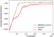
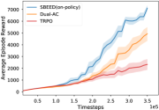
(a) Pendulum	(b) InvertedDoublePendulum

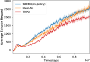
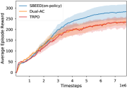
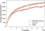
(c) HalfCheetah	(d) Swimmer	(e) Hopper

Figure 3: The results of SBEED against TRPO and Dual-AC in on-policy setting. Each plot shows average reward during training across $5$ random runs, with $50\%$ confidence interval. The x-axis is the number of training iterations. SBEED achieves better or comparable performance than TRPO and Dual-AC on all tasks.

We compared the SBEED to TRPO and Dual-AC in on-policy setting. We followed the same experimental set up as it is in off-policy setting. We ran the algorithm with $5$ random seeds and reported the average rewards with 50% confidence intervals. The empirical comparison results are illustrated in Figure 3. We can see that in all these tasks, the proposed SBEED achieves significantly better performance than the other algorithms. This can be thought as another ablation study that we switch off the “off-policy” in our algorithm. The empirical results demonstrate that the proposed algorithm is more flexible to way of the data sampled.

We set the step size to be $0.01$ and the batch size to be $52$ trajectories in each iteration in all algorithms in the on-policy setting. For TRPO, the CG damping parameter is set to be $10^{-4}$.

References

- Antos et al. (2008) Antos, András, Szepesvári, Csaba, and Munos, Rémi. Learning near-optimal policies with Bellman-residual minimization based fitted policy iteration and a single sample path. Machine Learning, 71(1):89–129, 2008.
- Asadi & Littman (2017) Asadi, Kavosh and Littman, Michael L. An alternative softmax operator for reinforcement learning. In ICML, pp. 243–252, 2017.
- Bach (2014) Francis R. Bach. Breaking the curse of dimensionality with convex neural networks. CoRR, abs/1412.8690, 2014. URL http://arxiv.org/abs/1412.8690.
- Baird (1995) Baird, Leemon. Residual algorithms: Reinforcement learning with function approximation. In ICML, pp. 30–37. Morgan Kaufmann, 1995.
- Bertsekas (2016) Bertsekas, Dimitri P. Nonlinear Programming. Athena Scientific, 3rd edition, 2016. ISBN 978-1-886529-05-2.
- Bertsekas & Tsitsiklis (1996) Bertsekas, Dimitri P. and Tsitsiklis, John N. Neuro-Dynamic Programming. Athena Scientific, September 1996. ISBN 1-886529-10-8.
- Borkar (1997) Vivek S Borkar. Stochastic approximation with two time scales. Systems & Control Letters, 29(5):291–294, 1997.
- Boyan (2002) Boyan, Justin A. Least-squares temporal difference learning. Machine Learning, 49(2):233–246, November 2002.
- Boyan & Moore (1995) Boyan, Justin A. and Moore, Andrew W. Generalization in reinforcement learning: Safely approximating the value function. In NIPS, pp. 369–376, 1995.
- Boyd & Vandenberghe (2004) Boyd, Stephen and Vandenberghe, Lieven. Convex Optimization. Cambridge University Press, Cambridge, England, 2004.
- Brockman et al. (2016) Brockman, Greg, Cheung, Vicki, Pettersson, Ludwig, Schneider, Jonas, Schulman, John, Tang, Jie, and Zaremba, Wojciech. OpenAI Gym, 2016. arXiv:1606.01540.
- Carrasco & Chen (2002) Carrasco, Marine and Chen, Xiaohong. Mixing and moment properties of various GARCH and stochastic volatility models. Econometric Theory, 18(1):17–39, 2002.
- Chen & Wang (2016) Chen, Yichen and Wang, Mengdi. Stochastic primal-dual methods and sample complexity of reinforcement learning. arXiv preprint arXiv:1612.02516, 2016.
- Dai et al. (2014) Dai, Bo, Xie, Bo, He, Niao, Liang, Yingyu, Raj, Anant, Balcan, Maria-Florina F, and Song, Le. Scalable kernel methods via doubly stochastic gradients. In NIPS, pp. 3041–3049, 2014.
- Dai et al. (2016) Bo Dai, Niao He, Yunpeng Pan, Byron Boots, and Le Song. Learning from conditional distributions via dual embeddings. CoRR, abs/1607.04579, 2016.
- Dai et al. (2018) Dai, Bo, Shaw, Albert, He, Niao, Li, Lihong, and Song, Le. Boosting the actor with dual critic. ICLR, 2018. arXiv:1712.10282.
- de Farias & Van Roy (2000) de Farias, Daniela Pucci and Van Roy, Benjamin. On the existence of fixed points for approximate value iteration and temporal-difference learning. Journal of Optimization Theory and Applications, 105(3):589–608, 2000.
- de Farias & Van Roy (2003) de Farias, Daniela Pucci and Van Roy, Benjamin. The linear programming approach to approximate dynamic programming. Operations Research, 51(6):850–865, 2003.
- Du et al. (2017) Du, Simon S., Chen, Jianshu, Li, Lihong, Xiao, Lin, and Zhou, Dengyong. Stochastic variance reduction methods for policy evaluation. In ICML, pp. 1049–1058, 2017.
- Fox et al. (2016) Fox, Roy, Pakman, Ari, and Tishby, Naftali. Taming the noise in reinforcement learning via soft updates. In UAI, 2016.
- Ghadimi & Lan (2013) Ghadimi, Saeed and Lan, Guanghui. Stochastic first-and zeroth-order methods for nonconvex stochastic programming. SIAM Journal on Optimization, 23(4):2341–2368, 2013.
- Ghadimi et al. (2016) Ghadimi, Saeed, Lan, Guanghui, and Zhang, Hongchao. Mini-batch stochastic approximation methods for nonconvex stochastic composite optimization. Mathematical Programming, 155(1-2):267–305, 2016.
- Gordon (1995) Gordon, Geoffrey J. Stable function approximation in dynamic programming. In ICML, pp. 261–268, 1995.
- Haarnoja et al. (2017) Haarnoja, Tuomas, Tang, Haoran, Abbeel, Pieter, and Levine, Sergey. Reinforcement learning with deep energy-based policies. In ICML, pp. 1352–1361, 2017.
- Haarnoja et al. (2018) Haarnoja, Tuomas, Zhou, Aurick, Abbeel, Pieter, and Levine, Sergey. Soft actor-critic: Off-policy maximum entropy deep reinforcement learning with a stochastic actor. arXiv preprint arXiv:1801.01290, 2018.
- Haussler (1995) Haussler, David. Sphere packing numbers for subsets of the Boolean -cube with bounded Vapnik-Chervonenkis dimension. Journal of Combinatorial Theory, Series A, 69(2):217–232, 1995.
- Henderson et al. (2018) Henderson, Peter, Islam, Riashat, Bachman, Philip, Pineau, Joelle, Precup, Doina, and Meger, David. Deep reinforcement learning that matters. In AAAI, 2018.
- Heusel et al. (2017) Heusel, Martin, Ramsauer, Hubert, Unterthiner, Thomas, Nessler, Bernhard, Klambauer, Günter, and Hochreiter, Sepp. Gans trained by a two time-scale update rule converge to a nash equilibrium. arXiv preprint arXiv:1706.08500, 2017.
- Kakade (2002) Kakade, Sham. A natural policy gradient. In NIPS, pp. 1531–1538, 2002.
- Kearns & Singh (2002) Kearns, Michael J. and Singh, Satinder P. Near-optimal reinforcement learning in polynomial time. Machine Learning, 49(2–3):209–232, 2002.
- Lagoudakis & Parr (2003) Lagoudakis, Michail G. and Parr, Ronald. Least-squares policy iteration. JMLR, 4:1107–1149, 2003.
- Lillicrap et al. (2015) Lillicrap, Timothy P, Hunt, Jonathan J, Pritzel, Alexander, Heess, Nicolas, Erez, Tom, Tassa, Yuval, Silver, David, and Wierstra, Daan. Continuous control with deep reinforcement learning. arXiv:1509.02971, 2015.
- Lin (1992) Lin, Long-Ji. Self-improving reactive agents based on reinforcement learning, planning and teaching. Machine Learning, 8(3–4):293–321, 1992.
- Liu et al. (2015) Liu, Bo, Liu, Ji, Ghavamzadeh, Mohammad, Mahadevan, Sridhar, and Petrik, Marek. Finite-sample analysis of proximal gradient td algorithms. In UAI, 2015.
- Liu et al. (2017) Liu, Yang, Ramachandran, Prajit, Liu, Qiang, and Peng, Jian. Stein variational policy gradient. In UAI, 2017.
- Macua et al. (2015) Macua, Sergio Valcarcel, Chen, Jianshu, Zazo, Santiago, and Sayed, Ali H. Distributed policy evaluation under multiple behavior strategies. IEEE Transactions on Automatic Control, 60(5):1260–1274, 2015.
- Maei (2011) Maei, Hamid Reza. Gradient Temporal-Difference Learning Algorithms. PhD thesis, University of Alberta, Edmonton, Alberta, Canada, 2011.
- Maei et al. (2010) Maei, Hamid Reza, Szepesvári, Csaba, Bhatnagar, Shalabh, and Sutton, Richard S. Toward off-policy learning control with function approximation. In ICML, pp. 719–726, 2010.
- Mahadevan et al. (2014) Mahadevan, Sridhar, Liu, Bo, Thomas, Philip S., Dabney, William, Giguere, Stephen, Jacek, Nicholas, Gemp, Ian, and Liu, Ji. Proximal reinforcement learning: A new theory of sequential decision making in primal-dual spaces. CoRR abs/1405.6757, 2014.
- Melo et al. (2008) Melo, Francisco S., Meyn, Sean P., and Ribeiro, M. Isabel. An analysis of reinforcement learning with function approximation. In ICML, pp. 664–671, 2008.
- Mnih et al. (2015) Mnih, Volodymyr, Kavukcuoglu, Koray, Silver, David, Rusu, Andrei A., Veness, Joel, Bellemare, Marc G., Graves, Alex, Riedmiller, Martin, Fidjeland, Andreas K., Ostrovski, Georg, Petersen, Stig, Beattie, Charles, Sadik, Amir, Antonoglou, Ioannis, King, Helen, Kumaran, Dharshan, Wierstra, Daan, Legg, Shane, and Hassabis, Demis. Human-level control through deep reinforcement learning. Nature, 518:529–533, 2015.
- Mnih et al. (2016) Mnih, Volodymyr, Badia, Adrià Puigdomènech, Mirza, Mehdi, Graves, Alex, Lillicrap, Timothy P., Harley, Tim, Silver, David, and Kavukcuoglu, Koray. Asynchronous methods for deep reinforcement learning. In ICML, pp. 1928–1937, 2016.
- Nachum et al. (2017) Nachum, Ofir, Norouzi, Mohammad, Xu, Kelvin, and Schuurmans, Dale. Bridging the gap between value and policy based reinforcement learning. In NIPS, pp. 2772–2782, 2017.
- Nachum et al. (2018) Nachum, Ofir, Norouzi, Mohammad, Xu, Kelvin, and Schuurmans, Dale. Trust-PCL: An off-policy trust region method for continuous control. In ICLR, 2018. arXiv:1707.01891.
- Nemirovski et al. (2009) Nemirovski, Arkadi, Juditsky, Anatoli, Lan, Guanghui, and Shapiro, Alexander. Robust stochastic approximation approach to stochastic programming. SIAM Journal on optimization, 19(4):1574–1609, 2009.
- Nesterov (2005) Nesterov, Yu. Smooth minimization of non-smooth functions. Mathematical programming, 103(1):127–152, 2005.
- Neu et al. (2017) Neu, Gergely, Jonsson, Anders, and Gómez, Vicenç. A unified view of entropy-regularized markov decision processes, 2017. arXiv:1705.07798.
- Ormoneit & Sen (2002) Ormoneit, Dirk and Sen, Śaunak. Kernel-based reinforcement learning. Machine Learning, 49:161–178, 2002.
- Puterman (2014) Puterman, Martin L. Markov Decision Processes: Discrete Stochastic Dynamic Programming. John Wiley & Sons, 2014.
- Rajeswaran et al. (2017) Rajeswaran, Aravind, Lowrey, Kendall, Todorov, Emanuel V., and Kakade, Sham M. Towards generalization and simplicity in continuous control. In NIPS, 2017.
- Rawlik et al. (2012) Rawlik, Konrad, Toussaint, Marc, and Vijayakumar, Sethu. On stochastic optimal control and reinforcement learning by approximate inference. In Robotics: Science and Systems VIII, 2012.
- Rubin et al. (2012) Rubin, Jonathan, Shamir, Ohad, and Tishby, Naftali. Trading value and information in MDPs. Decision Making with Imperfect Decision Makers, pp. 57–74, 2012.
- Rummery & Niranjan (1994) Rummery, G. A. and Niranjan, M. On-line Q-learning using connectionist systems. Technical Report CUED/F-INFENG/TR 166, Cambridge University Engineering Department, 1994.
- Schulman et al. (2015) Schulman, John, Levine, Sergey, Abbeel, Pieter, Jordan, Michael I, and Moritz, Philipp. Trust region policy optimization. In ICML, pp. 1889–1897, 2015.
- Schulman et al. (2017) Schulman, John, Abbeel, Pieter, and Chen, Xi. Equivalence between policy gradients and soft Q-learning, 2017. arXiv:1704.06440.
- Schweitzer & Seidmann (1985) Schweitzer, Paul J. and Seidmann, Abraham. Generalized polynomial approximations in Markovian decision processes. Journal of Mathematical Analysis and Applications, 110(2):568–582, 1985.
- Shapiro et al. (2009) Shapiro, Alexander, Dentcheva, Darinka, and Ruszczyński, Andrzej. Lectures on Stochastic Programming: Modeling and Theory. SIAM, 2009. ISBN 978-0-89871-687-0.
- Strehl et al. (2009) Strehl, Alexander L., Li, Lihong, and Littman, Michael L. Reinforcement learning in finite MDPs: PAC analysis. Journal of Machine Learning Research, 10:2413–2444, 2009.
- Sutton (1988) Sutton, Richard S. Learning to predict by the methods of temporal differences. Machine Learning, 3(1):9–44, 1988.
- Sutton (1996) Sutton, Richard S. Generalization in reinforcement learning: Successful examples using sparse coarse coding. In NIPS, pp. 1038–1044, 1996.
- Sutton & Barto (1998) Sutton, Richard S and Barto, Andrew G. Reinforcement Learning: An Introduction. MIT Press, 1998.
- Sutton et al. (2009) Sutton, Richard S., Maei, Hamid Reza, Precup, Doina, Bhatnagar, Shalabh, Silver, David, Szepesvári, Csaba, and Wiewiora, Eric. Fast gradient-descent methods for temporal-difference learning with linear function approximation. In ICML, pp. 993–1000, 2009.
- Todorov (2006) Todorov, Emanuel. Linearly-solvable Markov decision problems. In NIPS, pp. 1369–1376, 2006.
- Todorov et al. (2012) Todorov, Emanuel, Erez, Tom, and Tassa, Yuval. Mujoco: A physics engine for model-based control. In Intelligent Robots and Systems (IROS), 2012 IEEE/RSJ International Conference on, pp. 5026–5033. IEEE, 2012.
- Tsitsiklis & Van Roy (1997) Tsitsiklis, John N. and Van Roy, Benjamin. An analysis of temporal-difference learning with function approximation. IEEE Transactions on Automatic Control, 42:674–690, 1997.
- Wang (2017) Wang, Mengdi. Randomized linear programming solves the discounted Markov decision problem in nearly-linear running time. ArXiv e-prints, 2017.
- Watkins (1989) Watkins, Christopher J.C.H. Learning from Delayed Rewards. PhD thesis, King’s College, University of Cambridge, UK, 1989.
- Williams (1992) Williams, Ronald J. Simple statistical gradient-following algorithms for connectionist reinforcement learning. Machine Learning, 8:229–256, 1992.