Vector and Matrix Optimal Mass Transport:
Theory, Algorithm, and Applications

Abstract

In many applications such as color image processing, data has more than one piece of information associated with each spatial coordinate, and in such cases the classical optimal mass transport (OMT) must be generalized to handle vector-valued or matrix-valued densities. In this paper, we discuss the vector and matrix optimal mass transport and present three contributions. We first present a rigorous mathematical formulation for these setups and provide analytical results including existence of solutions and strong duality. Next, we present a simple, scalable, and parallelizable methods to solve the vector and matrix-OMT problems. Finally, we implement the proposed methods on a CUDA GPU and present experiments and applications.

1 Introduction

Optimal mass transport (OMT) is a subject with a long history. Started by Monge [41] and developed by many great mathematicians [34, 9, 28, 39, 33, 5, 46], the subject now has incredibly rich theory and applications. It has found numerous applications in different areas such as partial differential equations, probability theory, physics, economics, image processing, and control [26, 31, 55, 42, 17, 18, 13]. See also [50, 56, 2] and references therein.

However, in many applications such as color image processing, there is more than one piece of information associated with each spatial coordinate, and such data can be interpreted as vector-valued or matrix-valued densities. As the classical optimal mass transport works with scalar probability densities, such applications require a new notion of mass transport. For this purpose, Chen et al. [21, 20, 16, 14] recently developed a framework for vector-valued and matrix-valued optimal mass transport. See also [44, 43, 45, 27, 48, 58] for other different frameworks. For vector-valued OMT, potential applications include color image processing, multi-modality medical imaging, and image processing involving textures. For matrix-valued OMT, we have diffusion tensor imaging, multivariate spectral analysis, and stress tensor analysis.

Several mathematical aspects of vector and matrix-valued OMT were not addressed in the previous work [21, 20, 16]. As the first contribution of this paper, we present duality and existence results of the continuous vector and matrix-valued OMT problems along with rigorous problem formulations.

Although the classical theory of OMT is very rich, only recently has there been much attention to numerical methods to compute the OMT. Several recent work proposed algorithms to solve the $L^{2}$ OMT [3, 24, 7, 30, 6, 15, 19, 29] and the $L^{1}$ OMT [36, 53]. As the second contribution of this paper, we present first-order primal-dual methods to solve the vector and matrix-valued OMT problems. The methods simultaneously solve for both the primal and dual solutions (hence a primal-dual method) and are scalable as they are first-order methods. We also discuss the convergence of the methods.

As the third contribution of this paper, we implement the proposed method on a CUDA GPU and present several applications. The proposed algorithms’ simple structure allows us to effectively utilize the computing capability of the CUDA architecture, and we demonstrate this through our experiments. We furthermore release the code for scientific reproducibility.

The rest of the paper is structured as follows. In Section 2 we give a quick review of the classic OMT theory, which allows us to present the later sections in an analogous manner and thereby outline the similarities and differences. In Section 3 and Section 4 we present the vector and matrix-valued OMT problems and state a few theoretical results. In Section 5, we present and prove the analytical results. In Section 6, we discuss preliminaries we need for Section 7, where we present the algorithm. In Section 8, we present the experiments and applications.

2 Optimal mass transport

Let $\Omega\subset\mathbb{R}^{d}$ be a closed, convex, compact domain. Let $\lambda^{0}$ and $\lambda^{1}$ be nonnegative densities supported on $\Omega$ with unit mass, i.e., $\int_{\Omega}\lambda^{0}(\mathbf{x})\;d\mathbf{x}=\int_{\Omega}\lambda^{1}(\mathbf{x})\;d\mathbf{x}=1$. Let $\|\cdot\|$ denote any norm on $\mathbb{R}^{d}$.

In 1781, Monge posed the optimal mass transport (OMT) problem, which solves

$$\begin{split}\underset{T}{\text{minimize}}\quad\int_{\Omega}\|\mathbf{x}-T(\mathbf{x})\|\lambda^{0}(\mathbf{x})\;d\mathbf{x}.\end{split}$$ (1)

The optimization variable $T:\Omega\rightarrow\Omega$ is smooth, one-to-one, and transfers $\lambda^{0}(\mathbf{x})$ to $\lambda^{1}(\mathbf{x})$. The optimization problem (1) is nonlinear and nonconvex. In 1940, Kantorovich relaxed (1) into a linear (convex) optimization problem:

$$S(\lambda^{0},\lambda^{1})=\left(\begin{array}[]{ll}\underset{\pi}{\text{minimize}}&\int_{\Omega\times\Omega}\|\mathbf{x}-{\mathbf{y}}\|\pi(\mathbf{x},{\mathbf{y}})\;d\mathbf{x}d{\mathbf{y}}\\ \mbox{subject to}&\pi(\mathbf{x},{\mathbf{y}})\geq 0\\ &\int_{\Omega}\pi(\mathbf{x},{\mathbf{y}})\;d{\mathbf{y}}=\lambda^{0}(\mathbf{x})\\ &\int_{\Omega}\pi(\mathbf{x},{\mathbf{y}})\;d\mathbf{x}=\lambda^{1}({\mathbf{y}}).\end{array}\right)$$ (2)

The optimization variable $\pi$ is a joint nonnegative measure on $\Omega\times\Omega$ having $\lambda^{0}(\mathbf{x})$ and $\lambda^{1}({\mathbf{y}})$ as marginals. To clarify, $S(\lambda^{0},\lambda^{1})$ denotes the optimal value of (2).

2.1 Scalar optimal mass transport

The theory of optimal transport [28, 56, 57] remarkably points out that (2) is equivalent to the following flux minimization problem:

$$S(\lambda^{0},\lambda^{1})=\left(\begin{array}[]{ll}\underset{{\mathbf{u}}}{\text{minimize}}&\int_{\Omega}\|{\mathbf{u}}(\mathbf{x})\|\;d\mathbf{x}\\ \mbox{subject to}&\mathrm{div}_{\mathbf{x}}({\mathbf{u}})(\mathbf{x})=\lambda^{0}(\mathbf{x})-\lambda^{1}(\mathbf{x})\\ &{\mathbf{u}}(\mathbf{x})^{T}\mathbf{n}(\mathbf{x})=0,\,\,\mbox{for all }\begin{cases}\mathbf{x}\in\partial\Omega,\\ \text{$\mathbf{n}(\mathbf{x})$ normal to $\partial\Omega$},\end{cases}\end{array}\right)$$ (3)

where ${\mathbf{u}}=(u_{1},\dots,u_{d}):\Omega\rightarrow\mathbb{R}^{d}$ is the optimization variable and $\mathrm{div}_{\mathbf{x}}$ denote the (spatial) divergence operator. Although (3) and (2) are mathematically equivalent, (3) is much more computationally effective as its optimization variable ${\mathbf{u}}$ is much smaller when discretized.

It is worth mentioning that OMT in formulation (3) is very close to the problems in compressed sensing. Its objective function is homogeneous degree one and the constraint is linear. It can be observed that for characterizing the OMT, divergence operator in (3) play the key roles. Later on, we extend the definition of $L_{1}$ OMT problem by extending these differential operators into a general meaning.

The optimization problem (3) has the following dual problem:

$$S(\lambda^{0},\lambda^{1})=\left(\begin{array}[]{ll}\underset{\phi}{\text{maximize}}&\int_{\Omega}\phi(\mathbf{x})(\lambda^{1}(\mathbf{x})-\lambda^{0}(\mathbf{x}))\;d\mathbf{x}\\ \mbox{subject to}&\|\nabla_{\mathbf{x}}\phi(\mathbf{x})\|_{*}\leq 1\quad\text{for all }\mathbf{x}\in\Omega,\end{array}\right)$$ (4)

where the optimization and $\phi:\Omega\rightarrow\mathbb{R}$ is a function. We write $\|\cdot\|_{*}$ for the dual norm of $\|\cdot\|$.

It is well-known that, strong duality holds between (3) and (4) in the sense that the minimized and maximized objective values are equal [56]. Therefore, we take either (3) or (4) as the definition of $S$.

Rigorous definitions of the optimization problems (3) or (4) are somewhat technical. We skip this discussion, as scalar optimal mass transport is standard. In Section 5, we rigorously discuss the vector-OMT problems, so any rigorous discussion of the scalar-OMT problems can be inferred as a special case.

2.2 Theoretical properties

The algorithm we present in Section 7 is a primal-dual algorithm and, as such, finds solutions to both Problems (3) and (4). This is well-defined as both the primal and dual problems have solutions [56].

Write $\mathbb{R}_{+}$ for the set of nonnegative real numbers. Write $\mathcal{P}(\Omega,\mathbb{R})$ for the space of nonnegative densities supported on $\Omega$ with unit mass. We can use $S(\lambda^{0},\lambda^{1})$ as a distance measure between $\lambda^{0},\lambda^{1}\in\mathcal{P}(\Omega,\mathbb{R})$. The value $S:\mathcal{P}(\Omega,\mathbb{R})\times\mathcal{P}(\Omega,\mathbb{R})\rightarrow\mathbb{R}_{+}$ defines a metric on $\mathcal{P}(\Omega,\mathbb{R})$ [56].

3 Vector optimal mass transport

Next we discuss the vector-valued optimal transport, proposed recently in [20]. The basic idea is to combine scalar optimal mass transport with network flow problems [1].

Color image processing is the simplest application to think of for this setup. On an RGB color image, there are 3 values associated with each pixel. To generalize scalar-OMT to this setup, the cost for changing colors is defined with a graph. The edges represent the cost of changing one channel/color to another.

3.1 Gradient and divergence on graphs

Consider a connected, positively weighted, undirected graph ${\mathcal{G}}$ with $k$ nodes and $\ell$ edges. To define an incidence matrix for ${\mathcal{G}}$, we say an edge $\{i,j\}$ points from $i$ to $j$, i.e., $i\rightarrow j$, if $i<j$. This choice is arbitrary and does not affect the final result. With this edge orientation, the incidence matrix $D\in\mathbb{R}^{k\times\ell}$ is

$$D_{ie}=\left\{\begin{array}[]{ll}+1&\text{if edge $e=\{i,j\}$ for some node $j>i$}\\ -1&\text{if edge $e=\{j,i\}$ for some node $j<i$}\\ 0&\text{otherwise}.\end{array}\right.$$

For example, the incidence matrix of the graph of Figure 1 is

$$D=\begin{bmatrix}1&1&0&1&0\\ -1&0&1&0&0\\ 0&-1&-1&0&1\\ 0&0&0&-1&-1\end{bmatrix}.$$

Write $\Delta_{\mathcal{G}}=-D\operatorname{diag}\{1/c_{1}^{2},\cdots,1/c_{\ell}^{2}\}D^{T}$ for the (negative) graph Laplacian, where $1/c_{1}^{2},\cdots,1/c_{\ell}^{2}$ are the edge weights. The edge weights are defined so that and $c_{j}$ represents the cost of traversing edge $j$ for $j=1,\dots,\ell$.

Figure 1: Example graph with $k=4$ nodes and $\ell=5$ edges. To make $c_{j}$ the cost of traversing edge $j$, the edge weight is defined to be $1/c_{j}^{2}$ for $j=1,\dots,\ell$.

We define the gradient operator on ${\mathcal{G}}$ as $\nabla_{\mathcal{G}}x=\operatorname{diag}\{1/c_{1},\cdots,1/c_{\ell}\}D^{T}x$ and the divergence operator as $\mathrm{div}_{\mathcal{G}}y=-D\operatorname{diag}\{1/c_{1},\cdots,1/c_{\ell}\}y$. So the Laplacian can be rewritten as $\Delta_{\mathcal{G}}=\mathrm{div}_{\mathcal{G}}\nabla_{\mathcal{G}}$. Note that $\mathrm{div}_{\mathcal{G}}=-\nabla_{\mathcal{G}}^{*}$, where $\nabla_{\mathcal{G}}^{*}$ is the adjoint of $\nabla_{\mathcal{G}}$. This is in analogy with the usual spatial gradient and divergence operators [38, 22, 23, 20].

The edge weights of a graph ${\mathcal{G}}$ should be considered modeling parameters. In color image processing, for example, the edge weights of ${\mathcal{G}}$ represent the cost of changing one color to another, and they should be tuned to make results visually look best.

3.2 Vector optimal mass transport

We say $\accentset{\rightharpoonup}{\lambda}:\Omega\rightarrow{\mathbb{R}}^{k}_{+}$ is a nonnegative vector-valued density with unit mass if

$$\accentset{\rightharpoonup}{\lambda}(\mathbf{x})=\begin{bmatrix}\lambda_{1}(\mathbf{x})\\ \vdots\\ \lambda_{k}(\mathbf{x})\end{bmatrix},\qquad\int_{\Omega}\sum_{i=1}^{k}\lambda_{i}(\mathbf{x})\;d\mathbf{x}=1.$$

Assume $\accentset{\rightharpoonup}{\lambda}^{0}$ and $\accentset{\rightharpoonup}{\lambda}^{1}$ are nonnegative vector-valued densities supported on $\Omega$ with unit mass.

We define the optimal mass transport between vector-valued densities as

$$V(\accentset{\rightharpoonup}{\lambda}^{0},\accentset{\rightharpoonup}{\lambda}^{1})=\left(\begin{array}[]{ll}\underset{\accentset{\rightharpoonup}{{\mathbf{u}}},\accentset{\rightharpoonup}{w}}{\text{minimize}}&\int_{\Omega}\|\accentset{\rightharpoonup}{{\mathbf{u}}}(\mathbf{x})\|_{u}+\alpha\|\accentset{\rightharpoonup}{w}(\mathbf{x})\|_{w}\;d\mathbf{x}\\ \mbox{subject to}&\mathrm{div}_{\mathbf{x}}(\accentset{\rightharpoonup}{{\mathbf{u}}})(\mathbf{x})+\mathrm{div}_{\mathcal{G}}(\accentset{\rightharpoonup}{w}(\mathbf{x}))=\accentset{\rightharpoonup}{\lambda}^{0}(\mathbf{x})-\accentset{\rightharpoonup}{\lambda}^{1}(\mathbf{x})\\ &\accentset{\rightharpoonup}{{\mathbf{u}}}\text{ satisfies zero-flux b.c}.\end{array}\right)$$ (5)

where $\accentset{\rightharpoonup}{{\mathbf{u}}}:\Omega\rightarrow{\mathbb{R}}^{k\times d}$ and $\accentset{\rightharpoonup}{w}:\Omega\rightarrow{\mathbb{R}}^{\ell}$ are the optimization variables, $\alpha>0$ is a parameter, and $\|\cdot\|_{u}$ is a norm on $\mathbb{R}^{k\times d}$ and $\|\cdot\|_{w}$ is a norm on $\mathbb{R}^{\ell}$. The parameter $\alpha$ represents the relative importance of the two flux terms $\accentset{\rightharpoonup}{{\mathbf{u}}}$ and $\accentset{\rightharpoonup}{w}$. We write

$$\accentset{\rightharpoonup}{{\mathbf{u}}}=\begin{bmatrix}{\mathbf{u}}_{1}^{T}\\ \vdots\\ {\mathbf{u}}_{k}^{T}\end{bmatrix}\qquad\accentset{\rightharpoonup}{w}=\begin{bmatrix}w_{1}\\ \vdots\\ w_{\ell}\end{bmatrix}\qquad\mathrm{div}_{\mathbf{x}}(\accentset{\rightharpoonup}{{\mathbf{u}}})=\begin{bmatrix}\mathrm{div}_{\mathbf{x}}({\mathbf{u}}_{1})\\ \vdots\\ \mathrm{div}_{\mathbf{x}}({\mathbf{u}}_{k})\end{bmatrix}.$$

We call $\mathrm{div}_{\mathbf{x}}$ the spatial divergence operator. The zero-flux boundary condition is

$${\mathbf{u}}_{i}(\mathbf{x})^{T}\mathbf{n}(\mathbf{x})=0,\,\,\mbox{for all }\begin{cases}\mathbf{x}\in\partial\Omega,\\ \text{$\mathbf{n}(\mathbf{x})$ normal to $\partial\Omega$}.\end{cases}$$

for $i=1,\dots,k$. Note that $\accentset{\rightharpoonup}{w}$ has no boundary conditions.

The optimization problem (5) has the following dual problem:

$$V(\accentset{\rightharpoonup}{\lambda}^{0},\accentset{\rightharpoonup}{\lambda}^{1})=\left(\begin{array}[]{ll}\underset{\accentset{\rightharpoonup}{\phi}}{\text{maximize}}&\int_{\Omega}\langle\accentset{\rightharpoonup}{\phi}(\mathbf{x}),\accentset{\rightharpoonup}{\lambda}^{1}(\mathbf{x})-\accentset{\rightharpoonup}{\lambda}^{0}(\mathbf{x})\rangle\;d\mathbf{x}\\ \mbox{subject to}&\|\nabla_{\mathbf{x}}\accentset{\rightharpoonup}{\phi}(\mathbf{x})\|_{u*}\leq 1\\ &\|\nabla_{\mathcal{G}}\accentset{\rightharpoonup}{\phi}(\mathbf{x})\|_{w*}\leq\alpha\quad\text{for all }\mathbf{x}\in\Omega,\end{array}\right)$$ (6)

where the optimization variable $\accentset{\rightharpoonup}{\phi}:\Omega\rightarrow\mathbb{R}^{k}$ is a function. We write $\|\cdot\|_{u*}$ and $\|\cdot\|_{w*}$ for the dual norms of $\|\cdot\|_{u}$ and $\|\cdot\|_{w}$, respectively.

As stated in Theorem 1, strong duality holds between (5) and (6) in the sense that the minimized and maximized objective values are equal. Therefore, we take either (5) or (6) as the definition of $V$. In Section 5, we rigorously define the primal and dual problems and prove Theorem 1.

3.3 Theoretical properties

The algorithm we present in Section 7 is a primal-dual algorithm and, as such, finds solutions to both Problems (5) and (6). This is well-defined as both the primal and dual problems have solutions.

Theorem 1.

The (infinite dimensional) primal and dual optimization problems (5) and (6) have solutions, and their optimal values are the same, i.e., strong duality holds.

Write $\mathcal{P}(\Omega,\mathbb{R}^{k})$ for the space of nonnegative vector-valued densities supported on $\Omega$ with unit mass. We can use $V(\accentset{\rightharpoonup}{\lambda}^{0},\accentset{\rightharpoonup}{\lambda}^{1})$ as a distance measure between $\accentset{\rightharpoonup}{\lambda}^{0},\accentset{\rightharpoonup}{\lambda}^{1}\in\mathcal{P}(\Omega,\mathbb{R}^{k})$.

Theorem 2.

$V:\mathcal{P}(\Omega,\mathbb{R}^{k})\times\mathcal{P}(\Omega,\mathbb{R}^{k})\rightarrow\mathbb{R}_{+}$ defines a metric on $\mathcal{P}(\Omega,\mathbb{R}^{k})$.

4 Quantum gradient operator and matrix optimal mass transport

We closely follow the treatment in [21]. In particular, we define a notion of gradient on the space of Hermitian matrices and its dual, i.e., the (negative) divergence.

Some applications of matrix-OMT, such as diffusion tensor imaging, have real-valued data while some applications, such as multivariate spectral analysis, have complex-valued data [54]. To accommodate the wide range of applications, we develop the matrix-OMT with complex-valued matrices.

Write ${\mathcal{C}}$, ${\mathcal{H}}$, and ${\mathcal{S}}$ for the set of $k\times k$ complex, Hermitian, and skew-Hermitian matrices respectively. We write ${\mathcal{H}}_{+}$ for the set of $k\times k$ positive semidefinite Hermitian matrices, i.e., $M\in{\mathcal{H}}_{+}$ if $v^{*}Mv\geq 0$ for all $v\in\mathbb{C}^{k}$. Write $\operatorname{tr}$ for the trace, i.e. for any $M\in{\mathcal{H}}$, we have $\operatorname{tr}(M)=\sum^{k}_{i=1}M_{ii}$.

Write ${\mathcal{C}}^{N}$ for the block-column concatenation of $N$ matrices in ${\mathcal{C}}$, i.e., $\mathbf{Z}\in{\mathcal{C}}^{N}$ if $\mathbf{Z}=[Z_{1}^{*}\cdots Z_{N}^{*}]^{*}$ and $Z_{1},\dots,Z_{N}\in{\mathcal{C}}$. Define ${\mathcal{H}}^{N}$ and ${\mathcal{S}}^{N}$ likewise. For $X,Y\in{\mathcal{C}}$, we use the Hilbert-Schmidt inner product

$$\langle X,Y\rangle=\textrm{Re}\operatorname{tr}(XY^{*})=\sum^{k}_{i=1}\sum^{k}_{j=1}(\textrm{Re}X_{ij}\textrm{Re}Y_{ij}+\textrm{Im}X_{ij}\textrm{Im}Y_{ij}).$$

(This is the standard inner product when we view ${\mathcal{C}}$ as the real vector space $\mathbb{R}^{2n^{2}}$.) For $X\in{\mathcal{C}}$, we use the norm $\|X\|_{2}=(\langle X,X\rangle)^{1/2}$. For $\mathbf{X},\mathbf{Y}\in{\mathcal{C}}^{N}$, we use the inner product $\langle\mathbf{X},\mathbf{Y}\rangle=\sum_{s=1}^{N}\langle X_{s},Y_{s}\rangle$.

4.1 Quantum gradient and divergence operators

We define the gradient operator, given a $\mathbf{L}=[L_{1},\cdots,L_{\ell}]^{*}\in{\mathcal{H}}^{\ell}$, as

$$\nabla_{\mathbf{L}}:{\mathcal{H}}\rightarrow{{\mathcal{S}}}^{\ell},~{}~{}X\mapsto\left[\begin{array}[]{c}L_{1}X-XL_{1}\\ \vdots\\ L_{\ell}X-XL_{\ell}\end{array}\right].$$

Define the divergence operator as

$$\mathrm{div}_{\mathbf{L}}:{{\mathcal{S}}}^{\ell}\rightarrow{\mathcal{H}},~{}~{}Z=\left[\begin{array}[]{c}Z_{1}\\ \vdots\\ Z_{\ell}\end{array}\right]\mapsto\sum_{s=1}^{\ell}-L_{s}Z_{s}+Z_{s}L_{s}.$$

Note that $\mathrm{div}_{\mathbf{L}}=-\nabla_{\mathbf{L}}^{*}$, where $\nabla_{\mathbf{L}}^{*}$ is the adjoint of $\nabla_{\mathbf{L}}$. This is in analogy with the usual spatial gradient and divergence operators. Write $\Delta_{\mathbf{L}}=\mathrm{div}_{\mathbf{L}}\nabla_{\mathbf{L}}$. A standing assumption throughout, is that the null space of $\nabla_{\mathbf{L}}$, denoted by ${\rm ker}(\nabla_{\mathbf{L}})$, contains only scalar multiples of the identity matrix $I$.

The choice of $\mathbf{L}$ affects $\nabla_{\mathbf{L}}$ and, in turn, affects the induced metric. This definition of gradient operator is inspired by the Lindblad equation in Quantum Mechanics [21]. There has been some work on similar matrix optimal transport theories which focus on the applications in physics [11, 40]. However, how to appropriately choose $\mathbf{L}$ to fit a specific engineering application is still a topic of open research, and there is currently no established standard choice.

4.2 Matrix optimal mass transport

We say $\Lambda:\Omega\rightarrow{\mathcal{H}}_{+}$ is a nonnegative matrix-valued density with unit mass if

$$\int_{\Omega}\operatorname{tr}(\Lambda(\mathbf{x}))\;d\mathbf{x}=1.$$

Assume $\Lambda^{0}$ and $\Lambda^{1}$ are nonnegative matrix-valued densities supported on $\Omega$ with unit mass.

We define the optimal mass transport between matrix-valued densities as

$$M(\Lambda^{0},\Lambda^{1})=\left(\begin{array}[]{ll}\underset{{\mathbf{U}},{\mathbf{W}}}{\text{minimize}}&\int_{\Omega}\|{\mathbf{U}}(\mathbf{x})\|_{u}+\alpha\|{\mathbf{W}}(\mathbf{x})\|_{w}\;d\mathbf{x}\\ \mbox{subject to}&\mathrm{div}_{\mathbf{x}}({\mathbf{U}})(\mathbf{x})+\mathrm{div}_{\mathbf{L}}({\mathbf{W}}(\mathbf{x}))=\Lambda^{0}(\mathbf{x})-\Lambda^{1}(\mathbf{x})\\ &{\mathbf{U}}\text{ satisfies zero-flux b.c.}\end{array}\right)$$ (7)

where ${\mathbf{U}}:\Omega\rightarrow{\mathcal{H}}^{d}$ and ${\mathbf{W}}:\Omega\rightarrow{\mathcal{S}}^{\ell}$ are the optimization variables, $\alpha>0$ is a parameter, and $\|\cdot\|_{u}$ is a norm on ${\mathcal{H}}^{d}$ and $\|\cdot\|_{w}$ is a norm on ${\mathcal{S}}^{\ell}$. The parameter $\alpha$ represents the relative importance of the two flux terms ${\mathbf{U}}$ and ${\mathbf{W}}$. We write

$${\mathbf{U}}=\begin{bmatrix}U_{1}\\ \vdots\\ U_{d}\end{bmatrix}\qquad{\mathbf{W}}=\begin{bmatrix}W_{1}\\ \vdots\\ W_{\ell}\end{bmatrix}\quad{\mathbf{u}}_{ij}=\begin{bmatrix}(U_{1})_{ij}\\ \vdots\\ (U_{d})_{ij}\end{bmatrix}.$$

We define the spatial divergence as

$$\mathrm{div}_{\mathbf{x}}({\mathbf{U}})=\begin{bmatrix}\mathrm{div}_{\mathbf{x}}({\mathbf{u}}_{11})&\mathrm{div}_{\mathbf{x}}({\mathbf{u}}_{12})&\cdots&\mathrm{div}_{\mathbf{x}}({\mathbf{u}}_{1k})\\ \mathrm{div}_{\mathbf{x}}(\overline{{\mathbf{u}}}_{12})&\ddots&&\vdots\\ \vdots&&\ddots&\vdots\\ \mathrm{div}_{\mathbf{x}}(\overline{{\mathbf{u}}}_{1k})&\mathrm{div}_{\mathbf{x}}(\overline{{\mathbf{u}}}_{2k})&\cdots&\mathrm{div}_{\mathbf{x}}({\mathbf{u}}_{k,k})\end{bmatrix}.$$

The zero-flux boundary condition is

$${\mathbf{u}}_{ij}(\mathbf{x})^{T}\mathbf{n}(\mathbf{x})=0,\,\,\mbox{for all }\begin{cases}\mathbf{x}\in\partial\Omega,\\ \text{$\mathbf{n}(\mathbf{x})$ normal to $\partial\Omega$}.\end{cases}$$

for $i,j=1,\dots,k$. Note that ${\mathbf{W}}$ has no boundary conditions [16].

The optimization problem (7) has the following dual problem:

$$M(\Lambda^{0},\Lambda^{1})=\left(\begin{array}[]{ll}\underset{\Phi}{\text{maximize}}&\int_{\Omega}\langle\Phi(\mathbf{x}),\Lambda^{1}(\mathbf{x})-\Lambda^{0}(\mathbf{x})\rangle\;d\mathbf{x}\\ \mbox{subject to}&\|\nabla_{\mathbf{x}}\Phi(\mathbf{x})\|_{u*}\leq 1\\ &\|\nabla_{\mathbf{L}}\Phi(\mathbf{x})\|_{w*}\leq\alpha\quad\text{for all }\mathbf{x}\in\Omega,\end{array}\right)$$ (8)

where the optimization variable $\Phi:\Omega\rightarrow{\mathcal{H}}$ is a function. We write $\|\cdot\|_{u*}$ and $\|\cdot\|_{w*}$ for the dual norms of $\|\cdot\|_{u}$ and $\|\cdot\|_{w}$, respectively.

As stated in Theorem 3, strong duality holds between (7) and (8) in the sense that the minimized and maximized objective values are equal. Therefore we take either (7) or (8) as the definition of $M$.

In Section 5.6, we rigorously define the primal and dual problems. To prove the results on matrix-OMT (Theorems 3 and 4) one can take the arguments of Section 5 that prove the results on vector-OMT (Theorems 1 and 2) and change only the notation. We therefore simply point this out, instead of repeating same argument.

4.3 Theoretical properties

The algorithm we present in Section 7 is a primal-dual algorithm and, as such, finds solutions to both Problems (7) and (8). This is well-defined as both the primal and dual problems have solutions.

Theorem 3.

The (infinite dimensional) primal and dual optimization problems (7) and (8) have solutions, and their optimal values are the same, i.e., strong duality holds.

Write $\mathcal{P}(\Omega,{\mathcal{H}}_{+})$ for the space of nonnegative matrix-valued densities supported on $\Omega$ with unit mass. We can use $M(\Lambda^{0},\Lambda^{1})$ as a distance measure between $\Lambda^{0},\Lambda^{1}\in\mathcal{P}(\Omega,,{\mathcal{H}}_{+})$.

Theorem 4.

$M:\mathcal{P}(\Omega,{\mathcal{H}}_{+})\times\mathcal{P}(\Omega,{\mathcal{H}}_{+})\rightarrow\mathbb{R}_{+}$ defines a metric on $\mathcal{P}(\Omega,{\mathcal{H}}_{+})$.

5 Duality proof

In this section, we establish the theoretical results. For notational simplicity, we only prove the results for the vector-OMT primal and dual problems (5) and (6). Analogous results for the matrix-OMT primal and dual problems (7) and (8) follow from the same logic.

Although the classical scalar-OMT literature is very rich, standard techniques for proving scalar-OMT duality do not simply apply to our setup. For example, Villani’s proof of strong duality, presented as Theorem 1.3 of [56], relies on and works with the linear optimization formulation (2). However, our vector and matrix-OMT formulations directly generalize the flux formulation (3) and do not have formulations analogous to (2). We need a direct approach to analyze duality between the flux formulation and the dual (with one function variable), and we provide this in this section.

We further assume $\Omega\subset\mathbb{R}^{d}$ has a piecewise smooth boundary. Write $\Omega^{\circ}$ and $\partial\Omega$ for the interior and boundary of $\Omega$. For simplicity, assume $\Omega$ as full affine dimensions, i.e., $\overline{\Omega^{\circ}}=\Omega$.

The rigorous form of the dual problem (6) is

$$\begin{array}[]{ll}\underset{\accentset{\rightharpoonup}{\phi}\in W^{1,\infty}(\Omega,\mathbb{R}^{k})}{\text{maximize}}&\int_{\Omega}\langle\accentset{\rightharpoonup}{\phi}(\mathbf{x}),\accentset{\rightharpoonup}{\lambda}^{1}(\mathbf{x})-\accentset{\rightharpoonup}{\lambda}^{0}(\mathbf{x})\rangle\;d\mathbf{x}\\ \mbox{subject to}&\operatorname*{ess\,sup}_{\mathbf{x}\in\Omega}\|\nabla_{\mathbf{x}}\accentset{\rightharpoonup}{\phi}(\mathbf{x})\|_{u*}\leq 1\\ &\sup_{\mathbf{x}\in\Omega}\|\nabla_{\mathcal{G}}\accentset{\rightharpoonup}{\phi}(\mathbf{x})\|_{w*}\leq\alpha,\end{array}$$ (9)

where $W^{1,\infty}(\Omega,\mathbb{R}^{k})$ is the standard Sobolev space of functions from $\Omega$ to $\mathbb{R}^{k}$ with bounded weak gradients. That (9) has a solution directly follows from the Arzelà-Ascoli Theorem.

To rigorously define the primal problem (5) requires more definitions, and we do so later as (11).

5.1 Fenchel-Rockafellar duality

Let $L:X\rightarrow Y$ be a continuous linear map between locally convex topological vector spaces $X$ and $Y$, and let $f:X\rightarrow\mathbb{R}\cup\{\infty\}$ and $g:Y\rightarrow\mathbb{R}\cup\{\infty\}$ be lower-semicontinuous convex functions. Write

$$d^{\star}=\sup_{x\in X}\{-f(x)-g(Lx)\}\qquad p^{\star}=\inf_{y^{*}\in Y^{*}}\{f^{*}(L^{*}y^{*})+g^{*}(-y^{*})\},$$

where

$$f^{*}(x^{*})=\sup_{x\in X}\{\langle x^{*},x\rangle-f(x)\}\qquad g^{*}(y^{*})=\sup_{y\in Y}\{\langle y^{*},y\rangle-g(y)\}.$$

In this framework of Fenchel-Rockafellar duality, $d^{\star}\leq p^{\star}$, i.e., weak duality, holds unconditionally, and this is not difficult to prove. On the other hand, $d^{\star}=p^{\star}$, i.e., strong duality, requires additional assumptions and is more difficult to prove. The following theorem does this with a condition we can use.

Theorem 5.

[Theorem 17 and 18 [51]] If there is an $x\in X$ such that $f(x)<\infty$ and $g$ is bounded above in a neighborhood of $Lx$, then $p^{\star}=d^{\star}$. Furthermore, if $p^{\star}=d^{\star}<\infty$, the infimum of $\inf_{y^{*}\in Y^{*}}\{f^{*}(L^{*}y^{*})+g^{*}(-y^{*})\}$ is attained.

5.2 Spaces

Throughout this section, $\|\cdot\|_{1}$, $\|\cdot\|_{2}$, and $\|\cdot\|_{3}$ denote unspecified finite dimensional norms. As all finite dimensional norms are equivalent, we do not bother to precisely specify which norms they are.

Define

$$C(\Omega,\mathbb{R}^{k})=\left\{\accentset{\rightharpoonup}{\phi}:\Omega\rightarrow\mathbb{R}^{k}\,\,\Big{|}\,\,\accentset{\rightharpoonup}{\phi}\text{ is continuous},\,\|\accentset{\rightharpoonup}{\phi}\|_{\infty}=\max_{\mathbf{x}\in\Omega}\|\accentset{\rightharpoonup}{\phi}(\mathbf{x})\|_{1}<\infty\right\}.$$

Then $C(\Omega,\mathbb{R}^{k})$ is a Banach space equipped with the norm $\|\cdot\|_{\infty}$. We define $C(\Omega,\mathbb{R}^{k\times d})$ likewise. If $\accentset{\rightharpoonup}{\phi}\in C(\Omega,\mathbb{R}^{k})$ is continuously differentiable, $\nabla_{\mathbf{x}}\accentset{\rightharpoonup}{\phi}$ is defined on $\Omega^{\circ}$. We say $\nabla_{\mathbf{x}}\accentset{\rightharpoonup}{\phi}$ has a continuous extension to $\Omega$, if there is a $g\in C(\Omega,\mathbb{R}^{k\times d})$ such that $g|_{\Omega^{\circ}}=\nabla_{\mathbf{x}}\accentset{\rightharpoonup}{\phi}$. Define

$$C^{1}(\Omega,\mathbb{R}^{k})=\Big{\{}\accentset{\rightharpoonup}{\phi}:\mathbb{R}^{d}\rightarrow\mathbb{R}^{k}\,\,\big{|}\,\, \accentset{\rightharpoonup}{\phi}\text{ is continuously differentiable on }\Omega^{\circ},$$

$$\nabla_{\mathbf{x}}\accentset{\rightharpoonup}{\phi}\text{ has a continuous extension to }\Omega,$$

$$\|\accentset{\rightharpoonup}{\phi}\|_{\infty,\infty}=\max_{\mathbf{x}\in\Omega}\|\accentset{\rightharpoonup}{\phi}(\mathbf{x})\|_{2}+\sup_{\mathbf{x}\in\Omega}\|\nabla_{\mathbf{x}}\accentset{\rightharpoonup}{\phi}(\mathbf{x})\|_{3}<\infty\Big{\}}.$$

Then $C^{1}(\Omega,\mathbb{R}^{k})$ is a Banach space equipped with the norm $\|\cdot\|_{\infty,\infty}$.

Write $\mathcal{M}(\Omega,\mathbb{R}^{k})$ for the space of $\mathbb{R}^{k}$-valued signed finite Borel measures on $\Omega$, and define $\mathcal{M}(\Omega,\mathbb{R}^{k\times d})$ likewise. Write $(C(\Omega,\mathbb{R}^{k\times d}))^{*}$, $(C^{1}(\Omega,\mathbb{R}^{k}))^{*}$ for the topological dual of $C(\Omega,\mathbb{R}^{k\times d})$, $C^{1}(\Omega,\mathbb{R}^{k})$, respectively. The standard Riesz-Markov theorem tells us that $(C(\Omega,\mathbb{R}^{k\times d}))^{*}=\mathcal{M}(\Omega,\mathbb{R}^{k\times d})$.

Fully characterizing $(C^{1}(\Omega,\mathbb{R}^{k}))^{*}$ is hard, but we do not need to do so. Instead, we only use the following simple fact. Any $g\in\mathcal{M}(\Omega,\mathbb{R}^{k})$ defines the bounded linear map $\accentset{\rightharpoonup}{\phi}\mapsto\int_{\Omega}\langle\accentset{\rightharpoonup}{\phi}(\mathbf{x}),g(d\mathbf{x})\rangle$ for any $\accentset{\rightharpoonup}{\phi}\in C^{1}(\Omega,\mathbb{R}^{k})$. In other words, $\mathcal{M}(\Omega,\mathbb{R}^{k\times d})\subset(C^{1}(\Omega,\mathbb{R}^{k}))^{*}$ with the appropriate identification.

5.3 Operators

We redefine $\nabla_{\mathbf{x}}:C^{1}(\Omega,\mathbb{R}^{k})\rightarrow C(\Omega,\mathbb{R}^{k\times d})$ so that $\nabla_{\mathbf{x}}\accentset{\rightharpoonup}{\phi}$ is the continuous extension of the usual $\nabla_{\mathbf{x}}\accentset{\rightharpoonup}{\phi}$ to all of $\Omega$. This makes $\nabla_{\mathbf{x}}$ a bounded linear operator. Define the dual (adjoint) operator $\nabla_{\mathbf{x}}^{*}:\mathcal{M}(\Omega,\mathbb{R}^{k\times d})\rightarrow(C^{1}(\Omega,\mathbb{R}^{k}))^{*}$ by

$$\int_{\Omega}\langle\accentset{\rightharpoonup}{\phi}(\mathbf{x}),(\nabla_{\mathbf{x}}^{*}\accentset{\rightharpoonup}{{\mathbf{u}}})(d\mathbf{x})\rangle=\int_{\Omega}\langle(\nabla_{\mathbf{x}}\accentset{\rightharpoonup}{\phi})(\mathbf{x}),\accentset{\rightharpoonup}{{\mathbf{u}}}(d\mathbf{x})\rangle$$

for any $\accentset{\rightharpoonup}{\phi}\in C^{1}(\Omega,\mathbb{R}^{k})$ and $\accentset{\rightharpoonup}{{\mathbf{u}}}\in\mathcal{M}(\Omega,\mathbb{R}^{k\times d})$.

Define the $\nabla_{\mathcal{G}}$ (which is simply a multiplication by a $\mathbb{R}^{k\times\ell}$ matrix) as $\nabla_{\mathcal{G}}:C^{1}(\Omega,\mathbb{R}^{k})\rightarrow C(\Omega,\mathbb{R}^{\ell})$. Since $C^{1}(\Omega,\mathbb{R}^{\ell})\subset C(\Omega,\mathbb{R}^{\ell})$, there is nothing wrong with defining the range of $\nabla_{\mathcal{G}}$ to be $C(\Omega,\mathbb{R}^{\ell})$, and this still makes $\nabla_{\mathcal{G}}$ a bounded linear operator. Define the dual (adjoint) operator $\nabla_{\mathcal{G}}^{*}:\mathcal{M}(\Omega,\mathbb{R}^{\ell})\rightarrow(C^{1}(\Omega,\mathbb{R}^{k}))^{*}$ by identifying $\nabla_{\mathcal{G}}^{*}$ with the transpose of the matrix that defines $\nabla_{\mathcal{G}}$. Since $\nabla_{\mathcal{G}}^{*}$ is simply multiplication by a matrix, we can further say

$$\nabla_{\mathcal{G}}^{*}:\mathcal{M}(\Omega,\mathbb{R}^{\ell})\rightarrow\mathcal{M}(\Omega,\mathbb{R}^{k})\subset(C^{1}(\Omega,\mathbb{R}^{k}))^{*}.$$

We write $\mathrm{div}_{\mathcal{G}}=-\nabla_{\mathcal{G}}^{*}$.

5.4 Zero-flux boundary condition

Let $\accentset{\rightharpoonup}{\mathbf{m}}:\Omega\rightarrow\mathbb{R}^{k\times d}$ a smooth function. Then integration by parts tells us that

$$\int_{\Omega}\langle\nabla_{\mathbf{x}}\accentset{\rightharpoonup}{\varphi}(\mathbf{x}),\accentset{\rightharpoonup}{\mathbf{m}}(\mathbf{x})\rangle\;d\mathbf{x}=-\int_{\Omega}\langle\accentset{\rightharpoonup}{\varphi}(\mathbf{x}),\mathrm{div}_{\mathbf{x}}\accentset{\rightharpoonup}{\mathbf{m}}(\mathbf{x})\rangle\;d\mathbf{x}$$

holds for all smooth $\accentset{\rightharpoonup}{\varphi}:\Omega\rightarrow\mathbb{R}^{k}$ if and only if $\accentset{\rightharpoonup}{\mathbf{m}}(\mathbf{x})$ satisfies the zero-flux boundary condition, i.e., $\accentset{\rightharpoonup}{\mathbf{m}}(\mathbf{x})\mathbf{n}(\mathbf{x})=0$ for all $\mathbf{x}\in\partial\Omega$, where $\mathbf{n}(\mathbf{x})$ denotes the normal vector at $\mathbf{x}$. Here $\mathrm{div}_{\mathbf{x}}$ denotes the usual (spatial) divergence. To put it differently, $\nabla_{\mathbf{x}}^{*}=-\mathrm{div}_{\mathbf{x}}$ holds when the zero-flux boundary condition holds.

We generalize this notion to measures. We say $\accentset{\rightharpoonup}{{\mathbf{u}}}\in\mathcal{M}(\Omega,\mathbb{R}^{k\times d})$ satisfies the zero-flux boundary condition in the weak sense if there is a $\accentset{\rightharpoonup}{g}\in\mathcal{M}(\Omega,\mathbb{R}^{k})\subset(C^{1}(\Omega,\mathbb{R}^{k}))^{*}$ such that

$$\int_{\Omega}\langle\nabla_{\mathbf{x}}\accentset{\rightharpoonup}{\phi}(\mathbf{x}),\accentset{\rightharpoonup}{\mathbf{u}}(d\mathbf{x})\rangle=-\int_{\Omega}\langle\accentset{\rightharpoonup}{\phi}(\mathbf{x}),\accentset{\rightharpoonup}{g}(d\mathbf{x})\rangle$$

holds for all $\accentset{\rightharpoonup}{\phi}\in C^{1}(\Omega,\mathbb{R}^{k})$. In other words, $\accentset{\rightharpoonup}{{\mathbf{u}}}$ satisfies the zero-flux boundary condition if $\nabla_{\mathbf{x}}^{*}\accentset{\rightharpoonup}{{\mathbf{u}}}\in\mathcal{M}(\Omega,\mathbb{R}^{k})\subset(C^{1}(\Omega,\mathbb{R}^{k}))^{*}$. In this case, we write $\mathrm{div}_{\mathbf{x}}(\accentset{\rightharpoonup}{{\mathbf{u}}})=\accentset{\rightharpoonup}{g}$ and $\mathrm{div}_{\mathbf{x}}(\accentset{\rightharpoonup}{{\mathbf{u}}})=-\nabla_{\mathbf{x}}^{*}(\accentset{\rightharpoonup}{{\mathbf{u}}})$. This definition is often used in elasticity theory.

5.5 Duality

To establish duality, we view the dual problem (6) as the primal problem and obtain the primal problem (5) as the dual of the dual. We do this because the dual of $C(\Omega,\mathbb{R}^{k\times d})$ is known, while the dual of $\mathcal{M}(\Omega,\mathbb{R}^{k\times d})$ is difficult to characterize.

Consider the problem

$$\begin{array}[]{ll}\underset{\accentset{\rightharpoonup}{\phi}\in C^{1}(\Omega,\mathbb{R}^{k})}{\text{maximize}}&\int_{\Omega}\langle\accentset{\rightharpoonup}{\phi}(\mathbf{x}),\accentset{\rightharpoonup}{\lambda}^{1}(\mathbf{x})-\accentset{\rightharpoonup}{\lambda}^{0}(\mathbf{x})\rangle\;d\mathbf{x}\\ \mbox{subject to}&\|\nabla_{\mathbf{x}}\accentset{\rightharpoonup}{\phi}(\mathbf{x})\|_{u*}\leq 1\\ &\|\nabla_{\mathcal{G}}\accentset{\rightharpoonup}{\phi}(\mathbf{x})\|_{w*}\leq\alpha\quad\text{for all }\mathbf{x}\in\Omega,\end{array}$$ (10)

which is equivalent to (9). Define

$$L:C^{1}(\Omega,\mathbb{R}^{k}) \rightarrow C(\Omega,\mathbb{R}^{k\times d})\times C(\Omega,\mathbb{R}^{\ell})$$

$$\accentset{\rightharpoonup}{\phi} \mapsto(\nabla_{\mathbf{x}}\accentset{\rightharpoonup}{\phi},\nabla_{\mathcal{G}}\accentset{\rightharpoonup}{\phi})$$

and

$$g(a,b)=\left\{\begin{array}[]{ll}0&\text{if }\|a(\mathbf{x})\|_{u*}\leq 1,\,\|b(\mathbf{x})\|_{w*}\leq\alpha\text{ for all }\mathbf{x}\in\Omega\\ \infty&\text{otherwise}.\end{array}\right.$$

Rewrite (10) as

$$\begin{array}[]{ll}\underset{\accentset{\rightharpoonup}{\phi}\in C^{1}(\Omega,\mathbb{R}^{k})}{\text{maximize}}&\int_{\Omega}\langle\accentset{\rightharpoonup}{\phi}(\mathbf{x}),\accentset{\rightharpoonup}{\lambda}^{1}(\mathbf{x})-\accentset{\rightharpoonup}{\lambda}^{0}(\mathbf{x})\rangle\;d\mathbf{x}-g(L\accentset{\rightharpoonup}{\phi}),\end{array}$$

and consider its Fenchel-Rockafellar dual

$$\begin{array}[]{ll}\underset{\begin{subarray}{c}\accentset{\rightharpoonup}{{\mathbf{u}}}\in\mathcal{M}(\Omega,\mathbb{R}^{k\times d})\\ \accentset{\rightharpoonup}{w}\in\mathcal{M}(\Omega,\mathbb{R}^{k})\end{subarray}}{\text{minimize}}&\int_{\Omega}\|\accentset{\rightharpoonup}{{\mathbf{u}}}(\mathbf{x})\|_{u}+\alpha\|\accentset{\rightharpoonup}{w}(\mathbf{x})\|_{w}\;d\mathbf{x}\\ \mbox{subject to}&-\nabla_{\mathbf{x}}^{*}\accentset{\rightharpoonup}{{\mathbf{u}}}-\nabla_{\mathcal{G}}^{*}\accentset{\rightharpoonup}{w}=\accentset{\rightharpoonup}{\lambda}^{0}-\accentset{\rightharpoonup}{\lambda}^{1}\text{ as members of }(C^{1}(\Omega,\mathbb{R}^{k}))^{*}.\end{array}$$

The constraint

$$-\nabla_{\mathbf{x}}^{*}\accentset{\rightharpoonup}{{\mathbf{u}}}=\accentset{\rightharpoonup}{\lambda}^{0}-\accentset{\rightharpoonup}{\lambda}^{1}-\mathrm{div}_{\mathcal{G}}\accentset{\rightharpoonup}{w}\in\mathcal{M}(\Omega,\mathbb{R}^{k})\subset(C^{1}(\Omega,\mathbb{R}^{k}))^{*}$$

implies

$$-\nabla_{\mathbf{x}}^{*}\accentset{\rightharpoonup}{{\mathbf{u}}}\in\mathcal{M}(\Omega,\mathbb{R}^{k}),$$

i.e., $\accentset{\rightharpoonup}{{\mathbf{u}}}$ satisfies the zero-flux boundary condition.

We now state the rigorous form of the primal problem (5)

$$\begin{array}[]{ll}\underset{\begin{subarray}{c}\accentset{\rightharpoonup}{{\mathbf{u}}}\in\mathcal{M}(\Omega,\mathbb{R}^{k\times d})\\ \accentset{\rightharpoonup}{w}\in\mathcal{M}(\Omega,\mathbb{R}^{k})\end{subarray}}{\text{minimize}}&\int_{\Omega}\|\accentset{\rightharpoonup}{{\mathbf{u}}}(\mathbf{x})\|_{u}+\alpha\|\accentset{\rightharpoonup}{w}(\mathbf{x})\|_{w}\;d\mathbf{x}\\ \mbox{subject to}&\mathrm{div}_{\mathbf{x}}\accentset{\rightharpoonup}{{\mathbf{u}}}+\mathrm{div}_{\mathcal{G}}\accentset{\rightharpoonup}{w}=\accentset{\rightharpoonup}{\lambda}^{0}-\accentset{\rightharpoonup}{\lambda}^{1}\text{ as members of }\mathcal{M}(\Omega,\mathbb{R}^{k})\\ &\accentset{\rightharpoonup}{{\mathbf{u}}}\text{ satisfies zero-flux b.c in the weak sense}.\end{array}$$ (11)

The point $\accentset{\rightharpoonup}{\phi}=0$ satisfies the assumption of Theorem 5. Furthermore, it is easy to verify that the optimal value of the dual problem (6) is bounded. This implies strong duality, (11) is feasible, and (11) has a solution.

For $V(\accentset{\rightharpoonup}{\lambda}^{0},\accentset{\rightharpoonup}{\lambda}^{1})$ to be a metric, the 4 metric axioms must be satisfied. These are relatively straightforward to prove, and interested readers can find the argument in [16]. However, one more implicit axiom (not shown in previous works) must be shown: $V(\accentset{\rightharpoonup}{\lambda}^{0},\accentset{\rightharpoonup}{\lambda}^{1})<\infty$ for all $\accentset{\rightharpoonup}{\lambda}^{0},\accentset{\rightharpoonup}{\lambda}^{1}\in\mathcal{P}(\Omega,\mathbb{R}^{k})$. This follows from the fact that (11) has a solution. This completes the proof that $V:\mathcal{P}(\Omega,\mathbb{R}^{k})\times\mathcal{P}(\Omega,\mathbb{R}^{k})\rightarrow\mathbb{R}_{+}$ defines a metric.

5.6 Formal setup of Matrix-OMT

The rigorous form of the primal problem (7) is

$$\begin{array}[]{ll}\underset{\begin{subarray}{c}{\mathbf{U}}\in\mathcal{M}(\Omega,{\mathcal{H}}^{d})\\ {\mathbf{W}}\in\mathcal{M}(\Omega,{\mathcal{S}}^{\ell})\end{subarray}}{\text{minimize}}&\int_{\Omega}\|{\mathbf{U}}(\mathbf{x})\|_{u}+\alpha\|{\mathbf{W}}(\mathbf{x})\|_{w}\;d\mathbf{x}\\ \mbox{subject to}&\mathrm{div}_{\mathbf{x}}({\mathbf{U}})+\mathrm{div}_{\mathbf{L}}{\mathbf{W}}=\Lambda^{0}-\Lambda^{1}\text{ as members of }\mathcal{M}(\Omega,{\mathcal{H}})\\ &{\mathbf{U}}\text{ satisfies zero-flux b.c in the weak sense,}\end{array}$$

and the rigorous form of the dual problem (8) is

$$\begin{array}[]{ll}\underset{\Phi\in W^{1,\infty}(\Omega,{\mathcal{H}})}{\text{maximize}}&\int_{\Omega}\langle\Phi(\mathbf{x}),\Lambda^{1}(\mathbf{x})-\Lambda^{0}(\mathbf{x})\rangle\;d\mathbf{x}\\ \mbox{subject to}&\|\nabla_{\mathbf{x}}\Phi(\mathbf{x})\|_{u*}\leq 1\\ &\|\nabla_{\mathbf{L}}\Phi(\mathbf{x})\|_{w*}\leq\alpha\quad\text{for all }\mathbf{x}\in\Omega,\end{array}$$

where the measure and Sobolev spaces are defined similarly. Theorems 3 and 4 follow from the exact same reasoning as that of the vector counterparts.

6 Algorithmic preliminaries

Consider the Lagrangian for the vector optimal transport problems (5) and its dual (6)

$$L(\accentset{\rightharpoonup}{{\mathbf{u}}},\accentset{\rightharpoonup}{w},\accentset{\rightharpoonup}{\phi})= \int_{\Omega}\|\accentset{\rightharpoonup}{{\mathbf{u}}}(\mathbf{x})\|_{u}+\alpha\|\accentset{\rightharpoonup}{w}(\mathbf{x})\|_{w}\;d\mathbf{x}$$

$$\qquad\qquad+\int_{\Omega}\langle\accentset{\rightharpoonup}{\phi}(\mathbf{x}),\mathrm{div}_{\mathbf{x}}(\accentset{\rightharpoonup}{{\mathbf{u}}})(\mathbf{x})+\mathrm{div}_{\mathcal{G}}(\accentset{\rightharpoonup}{w}(\mathbf{x}))-\accentset{\rightharpoonup}{\lambda}^{0}(\mathbf{x})+\accentset{\rightharpoonup}{\lambda}^{1}(\mathbf{x})\rangle\;d\mathbf{x},$$ (12)

which is convex with respect to $\accentset{\rightharpoonup}{{\mathbf{u}}}$ and $\accentset{\rightharpoonup}{w}$ and concave with respect to $\phi$.

Finding a saddle point of (12) is equivalent to solving (5) and (6), when the primal problem (5) has a solution, the dual problem (6) has a solution, and the optimal values of (5) and (6) are equal. See [4, Theorem 7.1], [37, Theorem 2], or any reference on standard convex analysis such as [51] for further discussion on this point.

To solve the optimal transport problems, we discretize the continuous problems and apply PDHG method, which we soon describe, to solve the discretized convex-concave saddle point problem.

6.1 PDHG method

Consider the convex-concave saddle function

$$L(x,y,z)=f(x)+g(y)+\langle Ax+By,z\rangle-h(z),$$

where $f$, $g$, and $h$ are (closed and proper) convex functions and $x\in\mathbb{R}^{n}$, $y\in\mathbb{R}^{m}$, $z\in\mathbb{R}^{l}$, $A\in\mathbb{R}^{l\times n}$, and $B\in\mathbb{R}^{l\times m}$. Note $L$ is convex in $x$ and $y$ and concave in $z$. Assume $L$ has a saddle point and step sizes $\mu,\nu,\tau>0$ satisfy

$$1>\tau\mu\lambda_{\mathrm{max}}(A^{T}A)+\tau\nu\lambda_{\mathrm{max}}(B^{T}B).$$

Write $\|\cdot\|_{2}$ for the standard Euclidean norm. Then the method

$$x^{k+1} =\operatorname*{argmin}_{x\in\mathbb{R}^{n}}\left\{L(x,y^{k},z^{k})+\frac{1}{2\mu}\|x-x^{k}\|_{2}^{2}\right\}$$

$$y^{k+1} =\operatorname*{argmin}_{y\in\mathbb{R}^{m}}\left\{L(x^{k},y,z^{k})+\frac{1}{2\nu}\|y-y^{k}\|_{2}^{2}\right\}$$ (13)

$$z^{k+1} =\operatorname*{argmax}_{z\in\mathbb{R}^{l}}\left\{L(2x^{k+1}-x^{k},2y^{k+1}-y^{k},z)-\frac{1}{2\tau}\|z-z^{k}\|_{2}^{2}\right\}$$

converges to a saddle point. This method is called the Primal-Dual Hybrid Gradient (PDHG) method or the (preconditioned) Chambolle-Pock method [25, 12, 49].

PDHG can be interpreted as a proximal point method under a certain metric [32]. The quantity

$$R^{k}= \frac{1}{\mu}\|x^{k+1}-x^{k}\|_{2}^{2}+\frac{1}{\mu}\|y^{k+1}-y^{k}\|_{2}^{2}+\frac{1}{\tau}\|z^{k+1}-z^{k}\|_{2}^{2}$$

$$-2\langle z^{k+1}-z^{k},A(x^{k+1}-x^{k})+B(y^{k+1}-y^{k})\rangle.$$

is the fixed-point residual of the non-expansive mapping defined by the proximal point method. Therefore $R^{k}=0$ if and only if $(x^{k},y^{k},z^{k})$ is a saddle point of $L$, and $R^{k}$ decreases monotonically to $0$, cf., review paper [52]. We can use $R^{k}$ as a measure of progress and as a termination criterion.

6.2 Shrink operators

As the subproblems of PDHG (13) are optimization problems themselves, PDHG is most effective when these subproblems have closed-form solutions.

The problem definitions of scalar, vector, and matrix-OMT involve norms. For some, but not all, choices of norms, the “shrink” operators

$$\mathrm{shrink}(x^{0};\mu)=\operatorname*{argmin}_{x\in\mathbb{R}^{n}}\left\{\mu\|x\|+(1/2)\|x-x^{0}\|_{2}^{2}\right\}$$

have closed-form solutions. Therefore, when possible, it is useful to choose such norms for computational efficiency. Readers familiar with the compressed sensing or proximal methods literature may be familiar with this notion.

For the vector-OMT, we focus on norms

$$\|\accentset{\rightharpoonup}{{\mathbf{u}}}\|_{2}^{2}=\sum^{d}_{s=1}\|{\mathbf{u}}_{s}\|_{2}^{2}\qquad\|\accentset{\rightharpoonup}{{\mathbf{u}}}\|_{1,2}=\sum^{d}_{s=1}\|{\mathbf{u}}_{s}\|_{2}\qquad\|\accentset{\rightharpoonup}{{\mathbf{u}}}\|_{1}=\sum^{k}_{s=1}\|{\mathbf{u}}_{s}\|_{1}$$

for $\accentset{\rightharpoonup}{{\mathbf{u}}}\in\mathbb{R}^{k\times d}$ and

$$\|\accentset{\rightharpoonup}{w}\|_{2}^{2}=\sum^{\ell}_{s=1}(w_{s})^{2}\qquad\|\accentset{\rightharpoonup}{w}\|_{1}=\sum^{\ell}_{s=1}|w_{s}|$$

for $\accentset{\rightharpoonup}{w}\in\mathbb{R}^{\ell}$. The shrink operators of these norms have closed-form solutions.

For the matrix-OMT, we focus on norms

$$\|{\mathbf{U}}\|_{2}^{2}=\sum^{d}_{s=1}\sum^{k}_{i,j=1}|(U_{s})_{ij}|^{2}\,\|{\mathbf{U}}\|_{1}=\sum^{d}_{s=1}\sum^{k}_{i,j=1}|(U_{s})_{ij}|\quad\|{\mathbf{U}}\|_{\mathrm{1,nuc}}=\sum^{d}_{s=1}\|U_{s}\|_{\mathrm{nuc}}$$

for ${\mathbf{U}}\in{\mathcal{H}}^{d}$ and $\|\cdot\|_{2}$, $\|\cdot\|_{1}$, and $\|\cdot\|_{1,\mathrm{nuc}}$ for ${\mathbf{W}}\in{\mathcal{S}}^{\ell}$, which are defined likewise. The nuclear norm $\|\cdot\|_{\mathrm{nuc}}$ is the sum of the singular values. The shrink operators of these norms have closed-form solutions.

We provide further information and details on shrink operators in the appendix.

7 Algorithms

We now present simple and parallelizable algorithms for the OMT problems. These algorithms are, in particular, very well-suited for GPU computing.

In Section 7 and 8 we use an $n\times n$ discretization of the 2D domain $[0,1]\times[0,1]$ to obtain approximate solutions to the continuous problems. For simplicity of notation, we use the same symbol to denote the discretized variables and their continuous counterparts. Whether we are referring to the continuous variable or its discretization should be clear from context.

As mentioned in Section 6, these methods are the PDHG method applied to discretizations of the continuous problems. In the implementation, it is important to get the discretization at the boundary correct in order to respect the zero-flux boundary conditions. For interested readers, the details are provided in the appendix.

Instead of detailing the somewhat repetitive derivations of the algorithms in full, we simply show the key steps and arguments for the $\accentset{\rightharpoonup}{{\mathbf{u}}}$ update of vector-OMT. The other steps follow from similar logic.

When we discretize the primal and dual vector-OMT problems and apply PDHG to the discretized Lagrangian form of (12), we get

$$\accentset{\rightharpoonup}{{\mathbf{u}}}^{k+1} =\operatorname*{argmin}_{\accentset{\rightharpoonup}{{\mathbf{u}}}\in\mathbb{R}^{n\times n\times k\times d}}\left\{\sum_{ij}\|\accentset{\rightharpoonup}{{\mathbf{u}}}_{ij}\|_{u}+\langle\accentset{\rightharpoonup}{\phi}_{ij},(\mathrm{div}_{\mathbf{x}}{\mathbf{u}})_{ij}\rangle+\frac{1}{2\mu}\|\accentset{\rightharpoonup}{{\mathbf{u}}}_{ij}-\accentset{\rightharpoonup}{{\mathbf{u}}}^{k}_{ij}\|_{2}^{2}\right\}$$

$$=\operatorname*{argmin}_{\accentset{\rightharpoonup}{{\mathbf{u}}}\in\mathbb{R}^{n\times n\times k\times d}}\left\{\sum_{ij}\mu\|\accentset{\rightharpoonup}{{\mathbf{u}}}_{ij}\|_{u}-\mu\langle(\nabla_{\mathbf{x}}\accentset{\rightharpoonup}{\phi})_{ij},{\mathbf{u}}_{ij}\rangle+(1/2)\|\accentset{\rightharpoonup}{{\mathbf{u}}}_{ij}-\accentset{\rightharpoonup}{{\mathbf{u}}}_{ij}^{k}\|_{2}^{2}\right\}.$$

Since the minimization splits over the $i,j$ indices, we write

$$\accentset{\rightharpoonup}{{\mathbf{u}}}^{k+1}_{ij} =\operatorname*{argmin}_{\accentset{\rightharpoonup}{{\mathbf{u}}}_{ij}\in\mathbb{R}^{k\times d}}\left\{\mu\|\accentset{\rightharpoonup}{{\mathbf{u}}}_{ij}\|_{u}-\mu\langle(\nabla_{\mathbf{x}}\accentset{\rightharpoonup}{\phi})_{ij},{\mathbf{u}}_{ij}\rangle+(1/2)\|\accentset{\rightharpoonup}{{\mathbf{u}}}_{ij}-\accentset{\rightharpoonup}{{\mathbf{u}}}_{ij}^{k}\|_{2}^{2}\right\}$$

$$=\operatorname*{argmin}_{\accentset{\rightharpoonup}{{\mathbf{u}}}_{ij}\in\mathbb{R}^{k\times d}}\left\{\mu\|\accentset{\rightharpoonup}{{\mathbf{u}}}_{ij}\|_{u}+(1/2)\|\accentset{\rightharpoonup}{{\mathbf{u}}}_{ij}-(\accentset{\rightharpoonup}{{\mathbf{u}}}^{k}_{ij}+\mu(\nabla_{\mathbf{x}}\accentset{\rightharpoonup}{\phi})_{ij})\|_{2}^{2}\right\}$$

$$=\mathrm{shrink}(\accentset{\rightharpoonup}{{\mathbf{u}}}^{k}_{ij}+\mu(\nabla_{\mathbf{x}}\accentset{\rightharpoonup}{\phi})_{ij};\mu).$$

At the boundary, these manipulations need special care. When we incorporate ghost cells in our discretization, these seemingly cavalier manipulations are also correct on the boundary. We further explain the ghost cells and discretization in the appendix.

7.1 Scalar-OMT algorithm

The scalar-OMT algorithm can be viewed as a special case of vector-OMT or matrix-OMT algorithms. This scalar-OMT algorithm was presented in [36], but we restate it here for completeness.

First-order Method for S-OMT
	Input: Problem data $\lambda^{0}$, $\lambda^{1}$
			Initial guesses ${\mathbf{u}}^{0}$, $\phi^{0}$ and step sizes $\mu$, $\tau$
	Output: Optimal ${\mathbf{u}}^{\star}$ and $\phi^{\star}$
	for $k=1,2,\cdots$   (Iterate until convergence)
		${\mathbf{u}}^{k+1}_{ij}=\mathrm{shrink}({\mathbf{u}}_{ij}^{k}+\mu(\nabla\Phi^{k})_{ij},\mu)$   for $i,j=1,\dots,n$
		$\phi_{ij}^{k+1}=\phi_{ij}^{k}+\tau(\mathrm{div}_{\mathbf{x}}(2{\mathbf{u}}^{k+1}-{\mathbf{u}}^{k})_{ij}+\lambda^{1}_{ij}-\lambda^{0}_{ij})$   for $i,j=1,\dots,n$
	end

This method converges for step sizes $\mu,\tau>0$ that satisfy

$$1>\tau\mu\lambda_{\mathrm{max}}(-\Delta_{\mathbf{x}}).$$

For the particular setup of $\Omega=[0,1]\times[0,1]$ and $\Delta x=1/(n-1)$, the bound $\lambda_{\mathrm{max}}(-\Delta_{\mathbf{x}})\leq 8/(\Delta x)^{2}=8(n-1)^{2}$ is known. In our experiments, we use $\mu=1/(16\tau(n-1)^{2})$, a choice that ensures convergence for any $\tau>0$. We tune $\tau$ for the fastest convergence.

7.2 Vector-OMT algorithm

Write $\mathrm{shrink}_{u}$ and $\mathrm{shrink}_{w}$ for the shrink operators with respect to $\|\cdot\|_{u}$ and $\|\cdot\|_{w}$. The vector-OMT algorithm is as follows:

First-order Method for V-OMT
	Input: Problem data ${\mathcal{G}}$, $\accentset{\rightharpoonup}{\lambda}^{0}$, $\accentset{\rightharpoonup}{\lambda}^{1}$, $\alpha$
			Initial guesses $\accentset{\rightharpoonup}{{\mathbf{u}}}^{0}$, $\accentset{\rightharpoonup}{w}^{0}$, $\accentset{\rightharpoonup}{\phi}^{0}$ and step sizes $\mu$, $\nu$, $\tau$
	Output: Optimal $\accentset{\rightharpoonup}{{\mathbf{u}}}^{\star}$, $\accentset{\rightharpoonup}{w}^{\star}$, and $\accentset{\rightharpoonup}{\phi}^{\star}$
	for $k=1,2,\cdots$   (Iterate until convergence)
		$\accentset{\rightharpoonup}{{\mathbf{u}}}^{k+1}_{ij}=\mathrm{shrink}_{u}(\accentset{\rightharpoonup}{{\mathbf{u}}}_{ij}^{k}+\mu(\nabla\accentset{\rightharpoonup}{\phi}^{k})_{ij},\mu)$    for $i,j=1,\dots,n$
		$\accentset{\rightharpoonup}{w}^{k+1}_{ij}=\mathrm{shrink}_{w}(\accentset{\rightharpoonup}{w}^{k}_{ij}+\nu(\nabla_{\mathcal{G}}\accentset{\rightharpoonup}{\phi}^{k}_{ij}),\alpha\nu)$   for $i,j=1,\dots,n$
		$\accentset{\rightharpoonup}{\phi}_{ij}^{k+1}=\accentset{\rightharpoonup}{\phi}_{ij}^{k}+\tau(\mathrm{div}_{\mathbf{x}}(2\accentset{\rightharpoonup}{{\mathbf{u}}}^{k+1}-\accentset{\rightharpoonup}{{\mathbf{u}}}^{k})_{ij}+\mathrm{div}_{\mathcal{G}}(2\accentset{\rightharpoonup}{w}^{k+1}-\accentset{\rightharpoonup}{w}^{k})_{ij}+\accentset{\rightharpoonup}{\lambda}^{1}_{ij}-\accentset{\rightharpoonup}{\lambda}^{0}_{ij})$
				for $i,j=1,\dots,n$
	end

This method converges for step sizes $\mu,\nu,\tau>0$ that satisfy

$$1>\tau\mu\lambda_{\mathrm{max}}(-\Delta_{\mathbf{x}})+\tau\nu\lambda_{\mathrm{max}}(-\Delta_{\mathcal{G}}).$$

For the particular setup of $\Omega=[0,1]\times[0,1]$ and $\Delta x=1/(n-1)$, the bound $\lambda_{\mathrm{max}}(-\Delta_{\mathbf{x}})\leq 8(n-1)^{2}$ is known. Given a graph ${\mathcal{G}}$, we can compute $\lambda_{\mathrm{max}}(-\Delta_{\mathcal{G}})$ with a standard eigenvalue routine. In our experiments, we use $\mu=1/(32\tau(n-1)^{2})$ and $\nu=1/(4\tau\lambda_{\mathrm{max}}(-\Delta_{\mathcal{G}}))$, a choice that ensures convergence for any $\tau>0$. We tune $\tau$ for the fastest convergence.

7.3 Matrix-OMT algorithm

Write $\mathrm{shrink}_{u}$ and $\mathrm{shrink}_{w}$ for the shrink operators with respect to $\|\cdot\|_{u}$ and $\|\cdot\|_{w}$. The matrix-OMT algorithm is as follows:

First-order Method for M-OMT
	Input: Problem data $\mathbf{L}$, $\Lambda^{0}$, $\Lambda^{1}$, $\alpha$,
			Initial guesses ${\mathbf{U}}^{0}$, ${\mathbf{W}}^{0}$, $\Phi^{0}$ and step sizes $\mu$, $\nu$, $\tau$
	Output: Optimal ${\mathbf{U}}^{\star}$, ${\mathbf{W}}^{\star}$, and $\Phi^{\star}$
	for $k=1,2,\cdots$   (Iterate until convergence)
		${\mathbf{U}}^{k+1}_{ij}=\mathrm{shrink}_{u}({\mathbf{U}}_{ij}^{k}+\mu(\nabla\Phi^{k})_{ij},\mu)$      for $i,j=1,\dots,n$
		${\mathbf{W}}^{k+1}_{ij}=\mathrm{shrink}_{w}({\mathbf{W}}^{k}_{ij}+\nu(\nabla_{\mathbf{L}}\Phi^{k}_{ij}),\alpha\nu)$   for $i,j=1,\dots,n$
		$\Phi_{ij}^{k+1}=\Phi_{ij}^{k}+\tau(\mathrm{div}_{\mathbf{x}}(2{\mathbf{U}}^{k+1}-{\mathbf{U}}^{k})_{ij}+\mathrm{div}_{\mathbf{L}}(2{\mathbf{W}}^{k+1}-{\mathbf{W}}^{k})_{ij}+\Lambda^{1}_{ij}-\Lambda^{0}_{ij})$
				for $i,j=1,\dots,n$
	end

This method converges for step sizes $\mu,\nu,\tau>0$ that satisfy

$$1>\tau\mu\lambda_{\mathrm{max}}(-\Delta_{\mathbf{x}})+\tau\nu\lambda_{\mathrm{max}}(-\Delta_{\mathbf{L}}).$$

For the particular setup of $\Omega=[0,1]\times[0,1]$ and $\Delta x=1/(n-1)$, the bound $\lambda_{\mathrm{max}}(-\Delta_{\mathbf{x}})\leq 8(n-1)^{2}$ is known. Given $\mathbf{L}$, we can compute the value of $\lambda_{\mathrm{max}}(-\Delta_{\mathbf{L}})$ by explicitly forming a $k^{2}\times k^{2}$ matrix representing the linear operator $-\Delta_{\mathbf{L}}$ and applying a standard eigenvalue routine. In our experiments, we use $\mu=1/(32\tau(n-1)^{2})$ and $\nu=1/(4\tau\lambda_{\mathrm{max}}(-\Delta_{\mathbf{L}}))$, a choice that ensures convergence for any $\tau>0$. We tune $\tau$ for the fastest convergence.

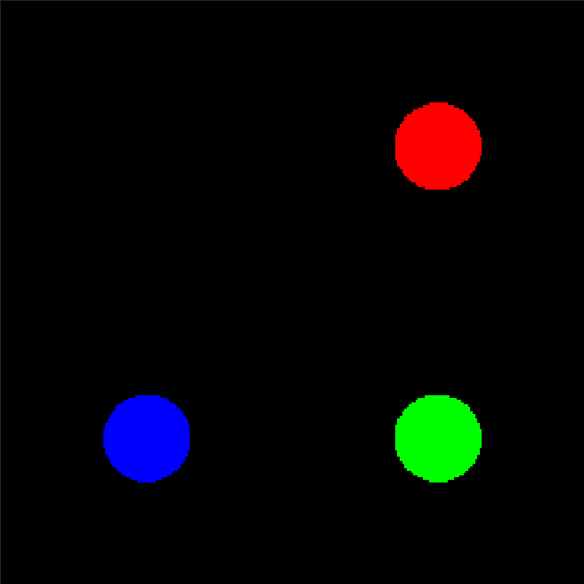
(a) $\accentset{\rightharpoonup}{\lambda}^{0}$

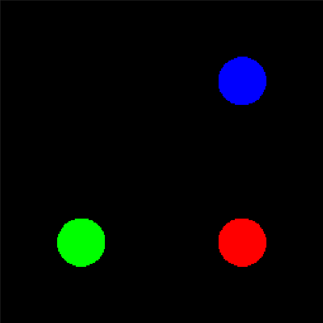
(b) $\accentset{\rightharpoonup}{\lambda}^{1}$

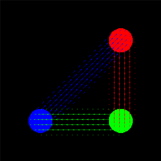
(c) Velocity field ${\mathbf{u}}$ with $c_{1}=1$, $c_{2}=1$, $c_{3}=1$, $\alpha=1$
and $\|\accentset{\rightharpoonup}{{\mathbf{u}}}\|_{1,2},\|\accentset{\rightharpoonup}{w}\|_{1}$. $V(\accentset{\rightharpoonup}{\lambda}^{0},\accentset{\rightharpoonup}{\lambda}^{1})=0.57$.

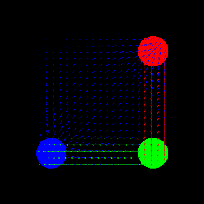
(d) Velocity field ${\mathbf{u}}$ with $c_{1}=1$, $c_{2}=1$, $c_{3}=1$, $\alpha=1$
and $\|\accentset{\rightharpoonup}{{\mathbf{u}}}\|_{1},\|\accentset{\rightharpoonup}{w}\|_{1}$. $V(\accentset{\rightharpoonup}{\lambda}^{0},\accentset{\rightharpoonup}{\lambda}^{1})=0.67$.

Figure 2: Color image vector-OMT example.

7.4 Parallelization

For the vector-OMT, the computation for the $\accentset{\rightharpoonup}{{\mathbf{u}}}$, $\accentset{\rightharpoonup}{w}$, and $\accentset{\rightharpoonup}{\phi}$ updates splits over the indices $(i,j)$, i.e., the computation splits pixel-by-pixel. Furthermore, the $\accentset{\rightharpoonup}{{\mathbf{u}}}$ and $\accentset{\rightharpoonup}{w}$ updates can be done in parallel. Parallel processors handing jobs split over $(i,j)$ must be synchronized before and after the $\accentset{\rightharpoonup}{\phi}$ update. The same is true for the scalar-OMT and matrix-OMT.

This highly parallel and regular algorithmic structure makes the proposed algorithms very well suited for CUDA GPUs. We demonstrate this through our experiments.

8 Examples

In this section, we provide example applications of vector and matrix-OMT with numerical tests to demonstrate the effectiveness of our algorithms. As mentioned in the introduction, potential applications of vector and matrix-OMT are broad. Here, we discuss two of the simplest applications.

We implemented the algorithm on C++ CUDA and ran it on a Nvidia GPU. For convenience, we MEXed this code, i.e., the code is made available as a Matlab function. For scientific reproducibility, we release this code.

8.1 Color images

Color images in RGB format is one of the more immediate examples of vector-valued densities. At each spatial position of a 2D color image, the color is represented as a combination of the three basic colors red (R), green (G), and blue (B). We allow any basic color to change to another basic color with cost $c_{1}$ for R to G, $c_{2}$ for R to B, and $c_{3}$ for G to B. So the graph ${\mathcal{G}}$ as described in Section 3.1 has 3 nodes and 3 edges.

Consider the two color images on the domain $\Omega=[0,1]\times[0,1]$ with $256\times 256$ discretization shown in Figures 2a and 2b. The initial and target densities $\accentset{\rightharpoonup}{\lambda}^{0}$ and $\accentset{\rightharpoonup}{\lambda}^{1}$ both have three disks at the same location, but with different colors. The optimal flux depends on the choice of norms. Figures 2c and 2d, show fluxes optimal with respect to different norms.

Whether it is optimal to spatially transport the colors or to change the colors depends on the parameters $c_{1},c_{2},c_{3},\alpha$ as well as the norms $\|\cdot\|_{u}$ and $\|\cdot\|_{w}$. With the parameters of Figure 3a it is optimal to spatially transport the colors, while with the parameters of Figure 3b it is optimal to change the colors.

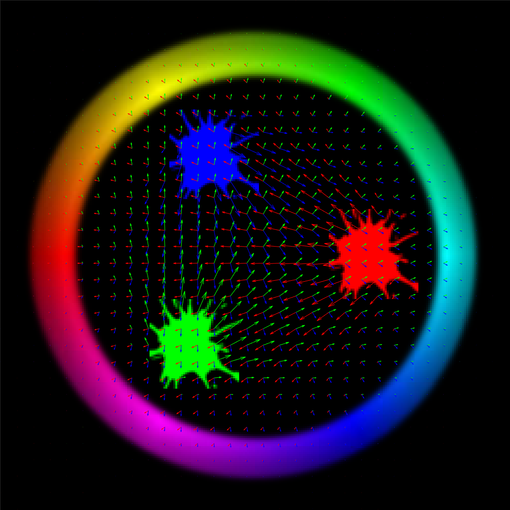
(a) $c_{1}=1,c_{2}=1,c_{3}=1,\alpha=10$.

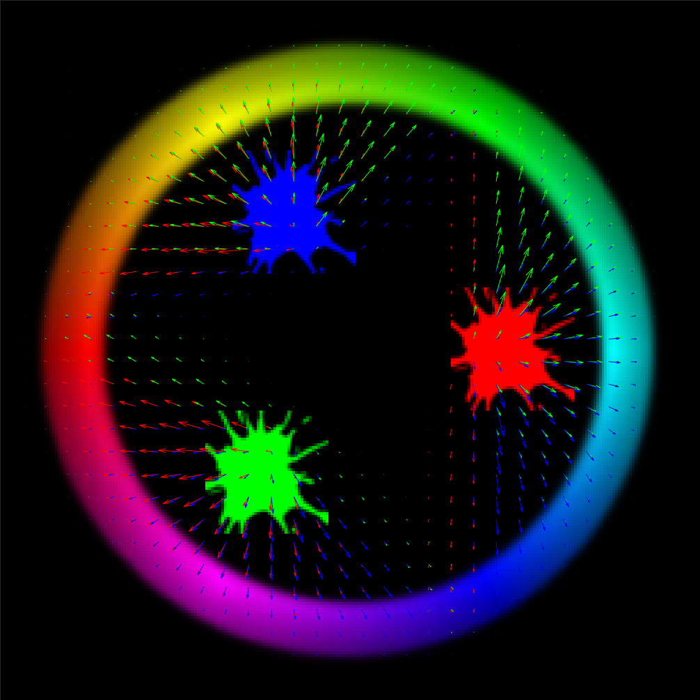
(b) $c_{1}=1,c_{2}=1,c_{3}=1,\alpha=0.1$.

Figure 3: Color image vector-OMT example, with a more complicated shape and norms $\|\accentset{\rightharpoonup}{{\mathbf{u}}}\|_{1,2},\|\accentset{\rightharpoonup}{w}\|_{2}$.

Finally, we test our algorithm on the setup of Figure 2c with grid sizes $32\times 32,64\times 64,128\times 128$, and $256\times 256$. Table 1 shows the number of iterations and runtime tested on a Nvidia Titan Xp GPU required to achieve a $10^{-3}$ precision, measured as the ratio between the duality gap and primal objective value.

Grid Size	Iteration count	Time per-iter	Iteration time	$\tau$	$V(\accentset{\rightharpoonup}{\lambda}^{0},\accentset{\rightharpoonup}{\lambda}^{1})$
$32\times 32$	$0.5\times 10^{4}$	$27\mu s$	$0.14s$	1	0.57
$64\times 64$	$0.5\times 10^{4}$	$27\mu s$	$0.14s$	1	0.57
$128\times 128$	$2\times 10^{4}$	$23\mu s$	$0.47s$	3	0.57
$256\times 256$	$2\times 10^{4}$	$68\mu s$	$1.36s$	3	0.57

Table 1: Computation cost for vector-OMT as a function of grid size.

8.2 Diffusion tensor imaging

Diffusion tensor imaging (DTI) is a technique used in magnetic resonance imaging. DTI captures orientations and intensities of brain fibers at each spatial position as ellipsoids and gives us a matrix-valued density. Therefore, the metric defined by the matrix-OMT provides a natural way to compare the differences between brain diffusion images. In Figure 4 we visualize diffusion tensor images by using colors to indicate different orientations of the tensors at each voxel. In this paper, we present simple 2D examples as a proof of concept and leave actual 3D imaging for a topic of future work.

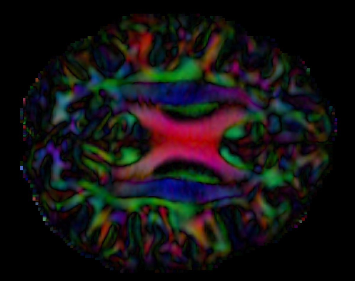
Figure 4: Example of 2D diffusion tensor images.

Consider three synthetic matrix-valued densities $\Lambda^{0}$, $\Lambda^{1}$, and $\Lambda^{2}$ in Figure 5. The densities $\Lambda^{0}$ and $\Lambda^{1}$ have mass at the same spatial location, but the ellipsoids have different shapes. The densities $\Lambda^{0}$ and $\Lambda^{2}$ have the same ellipsoids at different spatial locations.

We compute the distance between $\Lambda^{0}$, $\Lambda^{1}$, and $\Lambda^{2}$ for different parameters $\alpha$ and fixed ${\mathbf{L}}=[L_{1},L_{2}]^{*}$ with

$$L_{1}=\left[\begin{matrix}1&0&0\\ 0&2&0\\ 0&0&0\end{matrix}\right],\quad L_{2}=\left[\begin{matrix}1&1&1\\ 1&0&0\\ 1&0&0\end{matrix}\right].$$

Table 2, shows the results with $\|{\mathbf{U}}\|_{2}$ and $\|{\mathbf{W}}\|_{1}$ and grid size $128\times 128$. As we can see, whether $\Lambda^{0}$ is more “similar” to $\Lambda^{1}$ or $\Lambda^{2}$, i.e., whether $M(\lambda^{0},\lambda^{1})<M(\lambda^{0},\lambda^{2})$ or $M(\lambda^{0},\lambda^{1})>M(\lambda^{0},\lambda^{2})$, depends on whether the cost on ${\mathbf{U}}$, spatial transport, is higher than the cost on ${\mathbf{W}}$, changing the ellipsoids.

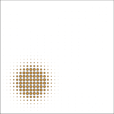
(a) $\Lambda^{0}$

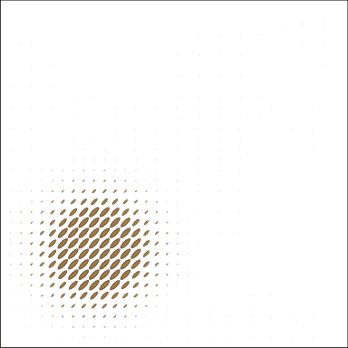
(b) $\Lambda^{1}$

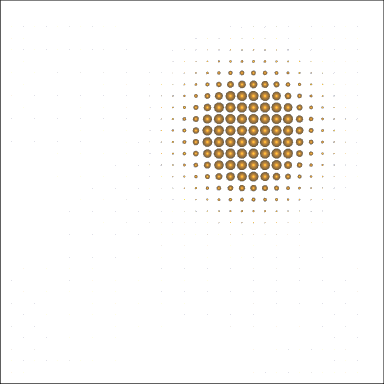
(c) $\Lambda^{2}$

Figure 5: Synthetic matrix-valued distributions.

Parameters	$M(\Lambda^{0},\Lambda^{1})$	$M(\Lambda^{0},\Lambda^{2})$	$M(\Lambda^{1},\Lambda^{2})$
$\alpha=10$	2.71	0.27	3.37
$\alpha=3$	0.81	0.27	1.08
$\alpha=1$	0.27	0.27	0.54
$\alpha=0.3$	0.081	0.27	0.35
$\alpha=0.1$	0.027	0.27	0.29

Table 2: Distances between the three images $\Lambda^{0},\Lambda^{1}$ and $\Lambda^{2}$.

Again, we test our algorithm on the setup of Figure 5 with $\alpha=1$ on grid sizes $32\times 32,64\times 64,128\times 128$, and $256\times 256$. Table 3 shows the number of iterations and runtime tested on a Nvidia Titan Xp GPU required to achieve a precision of $10^{-3}$, measured as the ratio between the duality gap and primal objective value.

Grid Size	Iteration count	Time per-iter	Iteration time	$\tau$	$M(\Lambda^{0},\Lambda^{1})$
$32\times 32$	$1\times 10^{4}$	$39\mu s$	$0.39s$	10	0.27
$64\times 64$	$1.5\times 10^{4}$	$39\mu s$	$0.59s$	10	0.27
$128\times 128$	$2\times 10^{4}$	$85\mu s$	$1.70s$	30	0.27
$256\times 256$	$4\times 10^{4}$	$330\mu s$	$13.2s$	60	0.27

Table 3: Computation cost for matrix-OMT as a function of grid size.

8.3 Discussion

The best choice of the norms for the vector and matrix-OMT problem depends on the application. In color image processing, for example, we recommend to use $\|\cdot\|_{1,2}$ for the $\|\cdot\|_{u}$ norm (which penalizes transport over space) since it respects the Euclidean geometry in the spatial domain and the penalties on different colors are decoupled. On the other hand, the choice for $\|\cdot\|_{w}$ norm (which penalizes change in color) seems to matter less. As another example, the nuclear norm is relevant to the problem of Michell trusses in structural mechanics [8].

The GPU implementation provides significant acceleration. For reference, we compared a serial CPU implementation against a parallel CUDA implementation for the scalar-OMT problem. When we run the method on a $1024\times 1024$ image, the serial implementation took $157.8ms$ per iteration while the CUDA implementation took $1.27ms$ per iteration. For computational problems with very simple parallelizable structures, $50$-fold to $150$-fold speedup is common. An Intel Core i7 CPU X990 @ 3.47GHz and Nvidia Titan Xp GPU were used for this experiment.

9 Conclusions

In this paper, we studied the extensions of Wasserstein-1 optimal transport to vector and matrix-valued densities. This extension, as a tool of applied mathematics, is interesting if the mathematics is sound, if the numerical methods are good, and if the applications are interesting. In this paper, we investigated all three concerns.

From a practical viewpoint, that we can solve vector and matrix-OMT problems of realistic sizes in modest time with GPU computing is the most valuable observation. Applying our algorithms to tackle real world problems in signal/imaging processing, medical imaging, and machine learning would be interesting directions of future research.

Another interesting direction of study is quadratic regularization. In general, the solutions to vector and matrix-OMT problems are not unique. However, the regularized version of (5)

$$\begin{array}[]{ll}\underset{\accentset{\rightharpoonup}{{\mathbf{u}}},\accentset{\rightharpoonup}{w}}{\text{minimize}}&\int_{\Omega}\|\accentset{\rightharpoonup}{{\mathbf{u}}}(\mathbf{x})\|_{u}+\alpha\|\accentset{\rightharpoonup}{w}(\mathbf{x})\|_{w}+\epsilon(\|\accentset{\rightharpoonup}{{\mathbf{u}}}(\mathbf{x})\|_{u}^{2}+\|\accentset{\rightharpoonup}{w}(\mathbf{x})\|_{w}^{2})\;d\mathbf{x}\\ \mbox{subject to}&\mathrm{div}_{\mathbf{x}}(\accentset{\rightharpoonup}{{\mathbf{u}}})(\mathbf{x})+\mathrm{div}_{\mathcal{G}}(\accentset{\rightharpoonup}{w}(\mathbf{x}))=\accentset{\rightharpoonup}{\lambda}^{0}(\mathbf{x})-\accentset{\rightharpoonup}{\lambda}^{1}(\mathbf{x})\\ &\accentset{\rightharpoonup}{{\mathbf{u}}}\text{ satisfies zero-flux b.c}\end{array}$$

is strictly convex and therefore has a unique solution. A similar regularization can be done for matrix-OMT. As discussed in [36, 53], this form of regularization is particularly useful as a slight modification to the proposed method solves the regularized problem.

Appendix A Discretization

Here, we describe the discretization for the vector-OMT problem (5) and (6). The discretization for the matrix-OMT problem is similar. We consider the 2D square domain, but (with more complicated notation) our approach immediately generalizes to more general domains. Again, we use the same symbol for the discretization and its continuous counterpart.

Consider a $n\times n$ discretization of $\Omega$ with finite difference $\Delta x$ in both $x$ and $y$ directions. Write the $x$ and $y$ coordinates of the points as $x_{1},\dots,x_{n}$ and $y_{1},\dots,y_{n}$. So we are approximating the domain $\Omega$ with $\{x_{1},\dots,x_{n}\}\times\{y_{1},\dots,y_{n}\}$. Write $C(x,y)$ for the $\Delta x\times\Delta x$ cube centered at $(x,y)$, i.e.,

$$C(x,y)=\{(x^{\prime},y^{\prime})\in\mathbb{R}^{2}\,|\,|x^{\prime}-x|\leq\Delta x/2\,,\,|y^{\prime}-y|\leq\Delta x/2\}\ .$$

We use a finite volume approximation for $\accentset{\rightharpoonup}{\lambda}^{0}$, $\accentset{\rightharpoonup}{\lambda}^{1}$, $\accentset{\rightharpoonup}{w}$ and $\accentset{\rightharpoonup}{\phi}$. Specifically, we write $\accentset{\rightharpoonup}{\lambda}^{0}\in\mathbb{R}^{n\times n\times k}$ with

$$\accentset{\rightharpoonup}{\lambda}^{0}_{ij}\approx\int_{C(x_{i},y_{j})}\accentset{\rightharpoonup}{\lambda}^{0}(x,y)\;dxdy,$$

for $i,j=1,\dots,n$. The discretizations $\accentset{\rightharpoonup}{\lambda}^{1},\accentset{\rightharpoonup}{\phi}\in\mathbb{R}^{n\times n\times k}$ and $\accentset{\rightharpoonup}{w}\in\mathbb{R}^{n\times n\times\ell}$ are defined the same way.

Write $\accentset{\rightharpoonup}{{\mathbf{u}}}=(\accentset{\rightharpoonup}{u}_{x},\accentset{\rightharpoonup}{u}_{y})$ for both the continuous variables and their discretizations. To be clear, the subscripts of $\accentset{\rightharpoonup}{u}_{x}$ and $\accentset{\rightharpoonup}{u}_{y}$ do not denote differentiation. We use the discretization $\accentset{\rightharpoonup}{u}_{x}\in\mathbb{R}^{(n-1)\times n\times k}$ and $\accentset{\rightharpoonup}{u}_{y}\in\mathbb{R}^{n\times(n-1)\times k}$. For $i=1,\dots,n-1$ and $j=1,\dots,n$

$$\accentset{\rightharpoonup}{u}_{x,ij}\approx\int_{C(x_{i}+\Delta x/2,y_{j})}\accentset{\rightharpoonup}{u}_{x}(x,y)\;dxdy,$$

and for $i=1,\dots,n$ and $j=1,\dots,n-1$

$$\accentset{\rightharpoonup}{u}_{y,ij}\approx\int_{C(x_{i},y_{j}+\Delta x/2)}\accentset{\rightharpoonup}{u}_{y}(x,y)\;dxdy.$$

In defining $\accentset{\rightharpoonup}{u}_{x}$ and $\accentset{\rightharpoonup}{u}_{y}$, the center points are placed between the $n\times n$ grid points to make the finite difference operator symmetric.

Define the discrete spacial divergence operator $\mathrm{div}_{\mathbf{x}}(\accentset{\rightharpoonup}{{\mathbf{u}}})\in\mathbb{R}^{n\times n\times k}$ as

$$\mathrm{div}_{\mathbf{x}}(\accentset{\rightharpoonup}{{\mathbf{u}}})_{ij}=\frac{1}{\Delta x}(\accentset{\rightharpoonup}{u}_{x,ij}-\accentset{\rightharpoonup}{u}_{x,(i-1)j}+\accentset{\rightharpoonup}{u}_{y,ij}-\accentset{\rightharpoonup}{u}_{y,i(j-1)}),$$

for $i,j=1,\dots,n$, where we mean $\accentset{\rightharpoonup}{u}_{x,0j}=\accentset{\rightharpoonup}{u}_{x,nj}=0$ for $j=1,\dots,n$ and $\accentset{\rightharpoonup}{u}_{y,i0}=\accentset{\rightharpoonup}{u}_{y,in}=0$ for $i=1,\dots,n$. This definition of $\mathrm{div}_{\mathbf{x}}(\accentset{\rightharpoonup}{{\mathbf{u}}})$ makes the discrete approximation consistent with the zero-flux boundary condition.

For $\accentset{\rightharpoonup}{\phi}\in\mathbb{R}^{n\times n}$, define the discrete gradient operator $\nabla_{\mathbf{x}}\accentset{\rightharpoonup}{\phi}=((\nabla\accentset{\rightharpoonup}{\phi})_{x},(\nabla\accentset{\rightharpoonup}{\phi})_{y})$ as

$$(\nabla\accentset{\rightharpoonup}{\phi})_{x,ij}=(1/\Delta x)\left(\accentset{\rightharpoonup}{\phi}_{i+1,j}-\accentset{\rightharpoonup}{\phi}_{i,j}\right) \quad\text{for }i=1,\dots,n-1,\,j=1,\dots,n$$

$$(\nabla\accentset{\rightharpoonup}{\phi})_{y,ij}=(1/\Delta x)\left(\accentset{\rightharpoonup}{\phi}_{i,j+1}-\accentset{\rightharpoonup}{\phi}_{i,j}\right) \quad\text{for }i=1,\dots,n,\,j=1,\dots,n-1.$$

So $(\nabla\accentset{\rightharpoonup}{\phi})_{x}\in\mathbb{R}^{(n-1)\times n\times k}$ and $(\nabla\accentset{\rightharpoonup}{\phi})_{y}\in\mathbb{R}^{n\times(n-1)\times k}$, and the $\nabla_{\mathbf{x}}$ is the transpose (as a matrix) of $-\mathrm{div}_{\mathbf{x}}$.

Ghost cells are convenient for both describing and implementing the method. This approach is similar to that of [36]. We redefine the variable $\accentset{\rightharpoonup}{{\mathbf{u}}}=(\accentset{\rightharpoonup}{u}_{x},\accentset{\rightharpoonup}{u}_{y})$ so that

$$\accentset{\rightharpoonup}{u}_{x,ij}=\left\{\begin{array}[]{ll}\accentset{\rightharpoonup}{u}_{x,ij}&\text{for }i<n\\ 0&\text{for }i=n\end{array}\right.\qquad\accentset{\rightharpoonup}{u}_{y,ij}=\left\{\begin{array}[]{ll}\accentset{\rightharpoonup}{u}_{y,ij}&\text{for }j<n\\ 0&\text{for }j=n\ ,\end{array}\right.$$

for $i,j=1,\dots,n$, and $\accentset{\rightharpoonup}{u}_{x},\accentset{\rightharpoonup}{u}_{y}\in\mathbb{R}^{n\times n\times k}$. We also redefine $\nabla\accentset{\rightharpoonup}{\phi}=((\nabla\accentset{\rightharpoonup}{\phi})_{x},(\nabla\accentset{\rightharpoonup}{\phi})_{y})$ so that

$$(\nabla\accentset{\rightharpoonup}{\phi})_{x,ij}=\left\{\begin{array}[]{ll}(\nabla\accentset{\rightharpoonup}{\phi})_{x,ij}&\text{for }i<n\\ 0&\text{for }i=n\end{array}\right.\qquad(\nabla\accentset{\rightharpoonup}{\phi})_{y,ij}=\left\{\begin{array}[]{ll}(\nabla\accentset{\rightharpoonup}{\phi})_{y,ij}&\text{for }j<n\\ 0&\text{for }j=n\ ,\end{array}\right.$$

for $i,j=1,\dots,n$, and $(\nabla\accentset{\rightharpoonup}{\phi})_{x},(\nabla\accentset{\rightharpoonup}{\phi})_{y}\in\mathbb{R}^{n\times n\times k}$.

With some abuse of notation, we write

$$\|\accentset{\rightharpoonup}{{\mathbf{u}}}\|_{u}=\sum^{n}_{i=1}\sum^{n}_{j=1}\|(\accentset{\rightharpoonup}{u}_{x,ij},\accentset{\rightharpoonup}{u}_{y,ij})\|_{u}\qquad\|\accentset{\rightharpoonup}{w}\|_{w}=\sum^{n}_{i=1}\sum^{n}_{j=1}\|\accentset{\rightharpoonup}{w}_{ij}\|_{w}.$$

Using this notation, we write the discretization of (5) as

$$\underset{\accentset{\rightharpoonup}{{\mathbf{u}}},\accentset{\rightharpoonup}{w}}{\text{minimize}} \|\accentset{\rightharpoonup}{{\mathbf{u}}}\|_{u}+\alpha\|\accentset{\rightharpoonup}{w}\|_{w}$$

subject to $$\mathrm{div}_{\mathbf{x}}(\accentset{\rightharpoonup}{{\mathbf{u}}})+\mathrm{div}_{\mathcal{G}}(\accentset{\rightharpoonup}{w})=\accentset{\rightharpoonup}{\lambda}^{0}-\accentset{\rightharpoonup}{\lambda}^{1},$$

where the boundary conditions are implicitly handled by the discretization.

Appendix B Shrink operators with closed-form solutions

Define $\mathrm{shrink}_{1}:\mathbb{C}\rightarrow\mathbb{C}$ as

$$\mathrm{shrink}_{1}(x;\mu) =\operatorname*{argmin}_{z\in\mathbb{C}}\left\{\mu|z|+(1/2)|z-x|^{2}\right\}$$

$$=\left\{\begin{array}[]{ll}(1-\mu/|x|)x&\text{ for }|x|\geq\mu\\ 0&\text{otherwise}\end{array}\right.$$

for $\mu>0$. Define $\mathrm{shrink}_{2}:\mathbb{C}^{k}\rightarrow\mathbb{C}^{k}$ as

$$\mathrm{shrink}_{2}(x;\mu) =\operatorname*{argmin}_{z\in\mathbb{C}^{k}}\left\{\mu\|z\|_{2}+(1/2)\|z-x\|^{2}_{2}\right\}$$

$$=\left\{\begin{array}[]{ll}(1-\mu/\|x\|_{2})x&\text{ for }\|x\|_{2}\geq\mu\\ 0&\text{otherwise}\end{array}\right.$$

for $\mu>0$, where $\|\cdot\|_{2}$ is the standard Euclidean norm. Define $\mathrm{shrink}_{\mathrm{nuc}}:{\mathcal{C}}\rightarrow{\mathcal{C}}$ as

$$\mathrm{shrink}_{\mathrm{nuc}}(X;\mu) =\operatorname*{argmin}_{Z\in{\mathcal{C}}}\left\{\mu\|Z\|_{*}+(1/2)\|Z-X\|^{2}_{2}\right\}$$

$$=U\operatorname{diag}\left([(\sigma_{1}-\mu)_{+},\dots,(\sigma_{n}-\mu)_{+}]\right)V^{T}$$

where $\|\cdot\|_{*}$ is the nuclear norm and $X=U\operatorname{diag}\left([\sigma_{1},\dots,\sigma_{n}]\right)V^{T}$ is the singular-value decomposition of $X$ [10]. If $x=(x_{1},x_{2},\dots,x_{k})$ and $\|x\|=\|x_{1}\|_{1}+\|x_{2}\|_{2}+\dots+\|x_{k}\|_{k}$ for some norms $\|\cdot\|_{1},\dots,\|\cdot\|_{k}$, then the shrink operators can be applied component-by-component. So if $\mathrm{shrink}_{1},\mathrm{shrink}_{2},\dots,\mathrm{shrink}_{k}$ are the individual shrink operators, then

$$\mathrm{shrink}(x;\mu)=\begin{bmatrix}\mathrm{shrink}_{1}(x_{1};\mu)\\ \mathrm{shrink}_{2}(x_{2};\mu)\\ \vdots\\ \mathrm{shrink}_{k}(x_{k};\mu)\\ \end{bmatrix}.$$

All shrink operators we consider in this paper can be built from these shrink operators. These ideas are well-known to the compressed sensing and proximal methods community [47].

However, there is a subtlety we must address when applying the shrink operators to matrix-OMT: the ${\mathbf{U}}$ update is defined as the minimization over ${\mathcal{H}}$, not all of ${\mathcal{C}}$, and the ${\mathbf{W}}$ update is defined as the minimization over ${\mathcal{S}}$, not all of ${\mathcal{C}}$. Fortunately, this is not a problem when we use unitarily invariant norms (such as the nuclear norm) thanks to the following lemma.

Lemma 1.

Let $M\in{\mathcal{H}}$ and $N\in{\mathcal{S}}$. Let $\|\cdot\|$ be a unitarily invariant norm, i.e., $\|UAV\|=\|A\|$ for any $A\in{\mathcal{C}}$, and $U,V\in{\mathcal{C}}$ unitary. Then

$$M^{+}=\operatorname*{argmin}_{A\in{\mathcal{H}}}\left\{\|A\|+\frac{1}{2}\|A-M\|^{2}_{2}\right\}=\operatorname*{argmin}_{A\in{\mathcal{C}}}\left\{\|A\|+\frac{1}{2}\|A-M\|^{2}_{2}\right\}$$

is Hermitian

$$N^{+}=\operatorname*{argmin}_{A\in{\mathcal{S}}}\left\{\|A\|+\frac{1}{2}\|A-N\|^{2}_{2}\right\}=\operatorname*{argmin}_{A\in{\mathcal{C}}}\left\{\|A\|+\frac{1}{2}\|A-N\|^{2}_{2}\right\}$$

is Skew-Hermitian.

Proof.

The minimum over ${\mathcal{H}}\subset{\mathcal{C}}$ is the same as the minimum over all of ${\mathcal{C}}$, if the minimum over all of ${\mathcal{C}}$ is in ${\mathcal{H}}$. Likewise, the minimum over ${\mathcal{S}}\subset{\mathcal{C}}$ is the same as the minimum over all of ${\mathcal{C}}$, if the minimum over all of ${\mathcal{C}}$ is in ${\mathcal{S}}$.

Write $\sigma:{\mathcal{C}}\rightarrow\mathbb{R}^{n}$ for the function that outputs singular values in decreasing order. Because of unitary invariance, we can write $\|X\|=f(\sigma(X))$, where $f:\mathbb{R}^{n}\rightarrow\mathbb{R}$ is a norm on $\mathbb{R}^{n}$ [59]. Furthermore, it’s subdifferential can be written as [35]

$$\partial\|\cdot\|(X)=\{U\operatorname{diag}(\mu)V^{T}\,|\,\mu\in(\partial f)(\sigma(X)),\,U\operatorname{diag}\sigma(X)V^{T}=X\text{ is SVD}\}.$$

Write $M=U\Sigma U^{T}$ for $M$’s eigenvalue decomposition, which is also its singular value decomposition. Define

$$\sigma^{+}=\operatorname*{argmin}_{s}\{f(s)+(1/2)\|s-\sigma(M)\|_{2}^{2}\},$$

which implies $0\in\partial f(\sigma^{+})+\sigma^{+}-\sigma(M)$. With this, we can verify that

$$0\in U\operatorname{diag}(\partial f(\sigma^{+}))U^{T}+U\operatorname{diag}(\sigma^{+})U^{T}-U\operatorname{diag}(\sigma(M))U^{T},$$

i.e., $U\operatorname{diag}(\sigma^{+})U^{T}$ satisfies the optimality conditions of the optimization problem that defines $M^{+}$. So $M^{+}=U\operatorname{diag}(\sigma^{+})U^{T}$, which is Hermitian.

Likewise, write $N=U\Lambda U^{T}$ for $N$’s eigenvalue decomposition. $N$ has orthonormal eigenvectors and its eigenvalues are purely imaginary. We separate out the magnitude and phase of $\Lambda$ and write $N=U\operatorname{diag}(\sigma(N))PU^{T}$. More precisely, $\sigma(N)=|\operatorname{diag}(\Lambda)|$ and $P$ is a diagonal matrix with diagonal components $\pm i$. Then the SVD of $N$ is $N=U\operatorname{diag}(\sigma(N))V^{T}$ where $PU^{T}=V^{T}$. With the same argument as before, we conclude that $N^{+}=U\operatorname{diag}(\sigma^{+})V^{T}$ for some $\sigma^{+}\in\mathbb{R}^{n}$. So $N^{+}=U\Lambda^{+}U^{T}$ where $\Lambda^{+}=\operatorname{diag}(\sigma^{+})P$ is diagonal and purely imaginary, and we conclude $N^{+}$ is skew-Hermitian. ∎

The norm $\|\cdot\|_{1}$ as described in Section 6.2, is not unitarily invariant. However, its shrink operator acts element-by-element, so it is easy to arrive at a conclusion similar to that of Lemma 1.

References

• [1] R. K. Ahuja, T. L. Magnanti, and J. B. Orlin, Network Flows: Theory, Algorithms, and Applications, Prentice Hall, 1993.
• [2] L. Ambrosio, N. Gigli, and G. Savaré, Gradient Flows: In Metric Spaces and in the Space of Probability Measures, Springer, 2006.
• [3] S. Angenent, S. Haker, and A. Tannenbaum, Minimizing flows for the Monge–Kantorovich problem, SIAM J. Math. Anal., 35 (2003), pp. 61–97.
• [4] H. H. Bauschke, R. I. Boţ, W. L. Hare, and W. M. Moursi, Attouch-Théra duality revisited: Paramonotonicity and operator splitting, J. Approx. Theory, 164 (2012), pp. 1065–1084.
• [5] J.-D. Benamou and Y. Brenier, A computational fluid mechanics solution to the Monge-Kantorovich mass transfer problem, Numer. Math., 84 (2000), pp. 375–393.
• [6] J.-D. Benamou, G. Carlier, M. Cuturi, L. Nenna, and G. Peyré, Iterative Bregman projections for regularized transportation problems, SIAM J. Sci. Comput., 37 (2015), pp. A1111–A1138.
• [7] J.-D. Benamou, B. D. Froese, and A. M. Oberman, Numerical solution of the optimal transportation problem using the Monge-Ampere equation, J. Comput. Phys., 260 (2014), pp. 107–126.
• [8] G. Bouchitté, W. Gangbo, and P. Seppecher, Michell trusses and lines of principal action, Mathematical Models and Methods in Applied Sciences, 18 (2008), pp. 1571–1603.
• [9] Y. Brenier, Polar factorization and monotone rearrangement of vector-valued functions, Comm. Pure Appl. Math., 44 (1991), pp. 375–417.
• [10] J.-F. Cai, E. J. Candès, and Z. Shen, A singular value thresholding algorithm for matrix completion, SIAM J. Optim., 20 (2010), pp. 1956–1982.
• [11] E. A. Carlen and J. Maas, Gradient flow and entropy inequalities for quantum markov semigroups with detailed balance, Journal of Functional Analysis, 273 (2017), pp. 1810–1869.
• [12] A. Chambolle and T. Pock, A first-order primal-dual algorithm for convex problems with applications to imaging, J. Math. Imaging Vis., 40 (2011), pp. 120–145.
• [13] Y. Chen, Modeling and Control of Collective Dynamics: From Schrödinger bridges to Optimal Mass Transport, PhD thesis, University of Minnesota, 2016.
• [14] Y. Chen, W. Gangbo, T. T. Georgiou, and A. Tannenbaum, On the matrix Monge-Kantorovich problem, arXiv, (2017).
• [15] Y. Chen, T. Georgiou, and M. Pavon, Entropic and displacement interpolation: a computational approach using the Hilbert metric, SIAM J. Appl. Math., 76 (2016), pp. 2375–2396.
• [16] Y. Chen, T. T. Georgiou, L. Ning, and A. Tannenbaum, Matricial Wasserstein-1 distance, IEEE control systems letters, 1 (2017), pp. 14–19.
• [17] Y. Chen, T. T. Georgiou, and M. Pavon, On the relation between optimal transport and Schrödinger bridges: A stochastic control viewpoint, J. Optim. Theory Appl., 169 (2016), pp. 671–691.
• [18] Y. Chen, T. T. Georgiou, and M. Pavon, Optimal transport over a linear dynamical system, IEEE Trans. Automat. Control, 62 (2017), pp. 2137–2152.
• [19] Y. Chen, T. T. Georgiou, and A. Tannenbaum, Interpolation of density matrices and matrix-valued measures: The unbalanced case, arXiv, (2016).
• [20] Y. Chen, T. T. Georgiou, and A. Tannenbaum, Vector-valued optimal mass transport, arXiv, (2016).
• [21] Y. Chen, T. T. Georgiou, and A. Tannenbaum, Matrix optimal mass transport: a quantum mechanical approach, IEEE Transactions on Automatic Control, (2017).
• [22] S.-N. Chow, W. Huang, Y. Li, and H. Zhou, Fokker-Planck equations for a free energy functional or Markov process on a graph, Arch. Ration. Mech. Anal., 203 (2012), pp. 969–1008.
• [23] S.-N. Chow, W. Li, and H. Zhou, Entropy dissipation of Fokker-Planck equations on graphs, arXiv, (2017).
• [24] M. Cuturi, Sinkhorn distances: Lightspeed computation of optimal transport, in Neural Inf. Process. Syst., 2013, pp. 2292–2300.
• [25] E. Esser, X. Zhang, and T. F. Chan, A general framework for a class of first order primal-dual algorithms for convex optimization in imaging science, SIAM J. Imaging Sci., 3 (2010), pp. 1015–1046.
• [26] L. C. Evans and W. Gangbo, Differential Equations Methods for the Monge-Kantorovich Mass Transfer Problem, American Mathematical Society, 1999.
• [27] J. H. Fitschen, F. Laus, and G. Steidl, Transport between RGB images motivated by dynamic optimal transport, J. Math. Imaging Vis., 56 (2016), pp. 409–429.
• [28] W. Gangbo and R. J. McCann, The geometry of optimal transportation, Acta Math., 177 (1996), pp. 113–161.
• [29] A. Genevay, M. Cuturi, G. Peyré, and F. Bach, Stochastic optimization for large-scale optimal transport, in Neural Inf. Process. Syst., 2016, pp. 3440–3448.
• [30] E. Haber and R. Horesh, A multilevel method for the solution of time dependent optimal transport, Numer. Math. Theory Methods Appl., 8 (2015), pp. 97–111.
• [31] S. Haker, L. Zhu, A. Tannenbaum, and S. Angenent, Optimal mass transport for registration and warping, Int. J. Comput. Vis., 60 (2004), pp. 225–240.
• [32] B. He and X. Yuan, Convergence analysis of primal-dual algorithms for a saddle-point problem: From contraction perspective, SIAM J. Imaging Sci., 5 (2012), pp. 119–149.
• [33] R. Jordan, D. Kinderlehrer, and F. Otto, The variational formulation of the Fokker–Planck equation, SIAM J. Math. Anal., 29 (1998), pp. 1–17.
• [34] L. V. Kantorovich, On the transfer of masses, Dokl. Akad. Nauk, 37 (1942), pp. 227–229.
• [35] A. Lewis, The convex analysis of unitarily invariant matrix functions., J. Convex Anal., 2 (1995), pp. 173–183.
• [36] W. Li, E. K. Ryu, S. Osher, W. Yin, and W. Gangbo, A parallel method for earth mover’s distance, J. Sci. Comput., (2017).
• [37] Y. Liu, E. K. Ryu, and W. Yin, A new use of Douglas-Rachford splitting for identifying infeasible, unbounded, and pathological conic programs, Mathematical Programming, (2018).
• [38] J. Maas, Gradient flows of the entropy for finite Markov chains, J. Funct. Anal., 261 (2011), pp. 2250–2292.
• [39] R. J. McCann, A convexity principle for interacting gases, Adv. Math., 128 (1997), pp. 153–179.
• [40] M. Mittnenzweig and A. Mielke, An entropic gradient structure for Lindblad equations and couplings of quantum systems to macroscopic models, Journal of Statistical Physics, 167 (2017), pp. 205–233.
• [41] G. Monge, Mémoire sur la théorie des déblais et des remblais, De l’Imprimerie Royale, 1781.
• [42] M. Mueller, P. Karasev, I. Kolesov, and A. Tannenbaum, Optical flow estimation for flame detection in videos, IEEE Trans. Image Process., 22 (2013), pp. 2786–2797.
• [43] L. Ning and T. T. Georgiou, Metrics for matrix-valued measures via test functions, in IEEE Conf. Decis. Control, IEEE, 2014, pp. 2642–2647.
• [44] L. Ning, T. T. Georgiou, and A. Tannenbaum, Matrix-valued Monge-Kantorovich optimal mass transport, in IEEE Conf. Decis. Control, IEEE, 2013, pp. 3906–3911.
• [45] L. Ning, T. T. Georgiou, and A. Tannenbaum, On matrix-valued Monge-Kantorovich optimal mass transport, IEEE Trans. Automat. Control, 60 (2015), pp. 373–382.
• [46] F. Otto and C. Villani, Generalization of an inequality by Talagrand and links with the logarithmic Sobolev inequality, J. Funct. Anal., 173 (2000), pp. 361–400.
• [47] N. Parikh and S. Boyd, Proximal algorithms, Found. Trends Optim., 1 (2014), pp. 127–239.
• [48] G. Peyre, L. Chizat, F.-X. Vialard, and J. Solomon, Quantum optimal transport for tensor field processing, European J. Appl. Math., (2017).
• [49] T. Pock and A. Chambolle, Diagonal preconditioning for first order primal-dual algorithms in convex optimization, IEEE Intern. Conf. Comput. Vis., (2011), pp. 1762–1769.
• [50] S. T. Rachev and L. Rüschendorf, Mass Transportation Problems: Volume I: Theory, vol. 1, Springer, 1998.
• [51] R. Rockafellar, Conjugate Duality and Optimization, Society for Industrial and Applied Mathematics, 1974.
• [52] E. K. Ryu and S. Boyd, Primer on monotone operator methods, Appl. Comput. Math., 15 (2016), pp. 3–43.
• [53] E. K. Ryu, W. Li, P. Yin, and S. Osher, Unbalanced and partial $L_{1}$ Monge-Kantorovich problem: A scalable parallel first-order method, J. Sci. Comput., (2017).
• [54] P. Stoica and R. L. Moses, Spectral Analysis of Signals, Prentice Hall, 2005.
• [55] E. Tannenbaum, T. Georgiou, and A. Tannenbaum, Signals and control aspects of optimal mass transport and the Boltzmann entropy, in IEEE Conf. Decis. Control, IEEE, 2010, pp. 1885–1890.
• [56] C. Villani, Topics in Optimal Transportation, American Mathematical Society, 2003.
• [57] C. Villani, Optimal Transport: Old and New, Springer, 2008.
• [58] T. Vogt and J. Lellmann, Measure-valued variational models with applications to diffusion-weighted imaging, Journal of Mathematical Imaging and Vision, (2018).
• [59] J. von Neumann, Some matrix inequalities and metrization of matric-space, Tomsk Univ. Rev., 1 (1937), pp. 286–300.