Improved Online Algorithm for Weighted Flow Time

Abstract

We discuss one of the most fundamental scheduling problem of processing jobs on a single machine to minimize the weighted flow time (weighted response time). Our main result is a $O(\log P)$-competitive algorithm, where $P$ is the maximum-to-minimum processing time ratio, improving upon the $O(\log^{2}P)$-competitive algorithm of Chekuri, Khanna and Zhu (STOC 2001). We also design a $O(\log D)$-competitive algorithm, where $D$ is the maximum-to-minimum density ratio of jobs. Finally, we show how to combine these results with the result of Bansal and Dhamdhere (SODA 2003) to achieve a $O(\log(\min(P,D,W)))$-competitive algorithm (where $W$ is the maximum-to-minimum weight ratio), without knowing $P,D,W$ in advance. As shown by Bansal and Chan (SODA 2009), no constant-competitive algorithm is achievable for this problem.

1 Introduction

We discuss the fundamental problem of online scheduling of jobs on a single machine. In this problem, a machine receives jobs over time, and the online algorithm decides which job to process at any point in time, allowing preemption as needed. Each of the jobs has a processing time (or volume) and a weight. We consider the weighted flow time cost function for this problem, in which the algorithm has to minimize the weighted sum over the jobs of the time between their arrival and their completion.

Define $P$ as the maximal ratio between the processing times of any two jobs, and $W$ as the maximal ratio between the weights of any two jobs. The first non-trivial algorithm for this problem was shown by Chekuri et al. [DBLP:conf/stoc/ChekuriKZ01], and is $O(\log^{2}P)$-competitive. Bansal and Dhamdhere [DBLP:journals/talg/BansalD07] showed a $O(\log W)$-competitive algorithm for this problem. A lower bound on competitiveness of
$\Omega(\min((\log W/\log\log W)^{\frac{1}{2}},(\log\log P/\log\log\log P)^{\frac{1}{2}}))$ was then shown by Bansal and Chan [DBLP:conf/soda/BansalC09].

An additional parameter of interest is $D$, which is the maximal ratio between the densities of any two jobs. This parameter has not been explored in any previous work, though the algorithm in [DBLP:conf/stoc/ChekuriKZ01] can be modified quite easily to yield a $O(\log^{2}D)$-competitive algorithm.

Our Results

Our main results are as follows:

• $O(\log P)$-competitive algorithm for weighted flow time on a single machine, improving upon the previous result of $O(\log^{2}P)$ in [DBLP:conf/stoc/ChekuriKZ01].

• $O(\log D)$-competitive algorithm. This algorithm is different from the $O(\log P)$-competitive algorithm.

• A combined algorithm which is $O(\log(\min(P,D,W)))$ competitive, without knowing $P,D,W$ in advance. This builds on the previous two algorithms and the algorithm of [DBLP:journals/talg/BansalD07].

Related Work

As mentioned above, for minimizing weighted flow time on a single machine, Chekuri et al. [DBLP:conf/stoc/ChekuriKZ01] presented a $O(\log^{2}P)$-competitive algorithm. The algorithm arranges all jobs in a table by their weight and density. The algorithm only processes jobs the weight of which is larger than the sum of the weights in the rectangle of lower density and lower weight jobs. In [DBLP:journals/talg/BansalD07], a $O(\log W)$-competitive algorithm is presented for this problem. This algorithm is based on the division of jobs into bins according to the logarithmic class of their weight, and then balancing the weights of those bins. A lower bound on algorithm competitiveness of $\Omega(\min((\log W/\log\log W)^{\frac{1}{2}},(\log\log P/\log\log\log P)^{\frac{1}{2}}))$ was shown in [DBLP:conf/soda/BansalC09]. Typically, one assumes that $P$ and $W$ are bounded and that the number of jobs may be arbitrarily large (unbounded). In the case that the number of jobs is small, it is shown in [DBLP:journals/talg/BansalD07] how to use the $O(\log W)$ competitive algorithm to construct a $O(\log P+\log n)$-competitive algorithm, with $n$ being the number of jobs released. Note that the competitive ratio of this algorithm is unbounded as a function of $P$. For the offline problem, Chekuri and Khanna [Chekuri:2002:ASP:509907.509954] showed a quasi-polynomial time approximation scheme. Bansal [Bansal:2005:MFT:2308916.2309425] later extended this result to a constant number of machines.

For a single machine in the unweighted case, a classic result from [NAV:NAV3800030106] states that the shortest remaining processing time algorithm is optimal. For the case of $m$ identical machines, and a set of $n$ jobs, Leonardi and Raz [Leonardi:1997:ATF:258533.258562] showed that SRPT is $O(\log(\min(P,\frac{n}{m})))$-competitive, and that this is optimal. Awerbuch et al. [doi:10.1137/S009753970037446X] presented a $O(\log(\min(P,n)))$-competitive algorithm in which jobs do not migrate machines. An algorithm with immediate dispatching (and no migration) with similar guarantees was presented in [Avrahami:2003:MTF:777412.777415]. In contrast to those positive results, for the case of weighted flow time on multiple machines, Chekuri et al. [DBLP:conf/stoc/ChekuriKZ01] showed a $\Omega(\min(\sqrt{P},\sqrt{W},(\frac{n}{m})^{\frac{1}{4}}))$ lower bound on competitiveness for $m>1$ machines, making the problem intractable.

Competitive algorithms also exist for unweighted flow time on related machines [DBLP:conf/icalp/GargK06, DBLP:conf/stoc/GargK06]. For the case of unweighted flow time for machines with restricted assignment, no online algorithm with a bounded competitive ratio exists [DBLP:conf/focs/GargK07].

In the resource augmentation problem, the single machine weighted flow time problem becomes significally easier. In [BECCHETTI2006339], a $(1+\frac{1}{\epsilon})$-competitive algorithm is given for a $(1+\epsilon)$-speed model. An algorithm with a similar guarantee was given in [DBLP:journals/talg/BansalD07] for the non-clairvoyant setting. A competitive algorithm is also known for weighted flow time in unrelated machines [DBLP:conf/stoc/ChadhaGKM09]. Additional work has been done on weighted flow time for unrelated machines with resource augmentation in the offline model (see e.g. [DBLP:conf/stoc/ChekuriGKK04, doi:10.1137/1.9781611973099.97]).

Our Technique

Processing-time ratio algorithm. Our $O(\log P)$ algorithm rounds the weights of incoming jobs to a power of $2$, and assigns them into power-of-$2$ bins according to their processing time. That is, bin $i$ contains jobs whose initial processing time is in the range $[2^{i},2^{i+1})$. Note that jobs never move between bins.

To describe the algorithm, we utilize a visualization of the algorithms state, as shown in figure 4.1. We view each job as a rectangular container, such that the height of the rectangle is the weight of the job, and its area is $2^{i+1}$. The volume of the job can be viewed as liquid within that container. When a job is being processed, the amount of liquid is reduced from the top. A horizontal dotted line runs through the middle of the container. This line helps to observe the volume covered by a bar, a concept used in the algorithm’s analysis.

Inside each bin, jobs of higher weight have a higher priority for processing. For jobs of the same weight, the jobs are ordered according to their density, such that lower density jobs get priority. This priority is illustrated by the rectangular containers of the jobs being stacked on top of one another, such that a higher job in the stack has higher priority.

At any point in time, the algorithm chooses a bin from which to process the uppermost job. At each point in time, each bin is assigned a score, such that the bin with the highest score is processed. In [DBLP:journals/talg/BansalD07], the score assigned to each bin is the total weight of the jobs in that bin. In our algorithm, the score is more complex. All jobs except the top job add their weight to the total score of the bin. The top job adds to the score of the bin either its complete weight, if it has high remaining processing time, or half of it, if it has low remaining processing time. While this modification seems odd, it is crucial for the proof. This can lead to some interesting behavior: for example, a job can be preempted during processing because its processing time has decreased below the threshold, lowering the score of its bin. This preemption is not due to any external event; no job has been released to trigger it.

The outline of our proof is inspired by [DBLP:journals/talg/BansalD07]. In our proof, we use the concept of volume covered by a bar. We place a horizontal bar at some height $x$, as shown in figure 4.1. If the bar lies over the top of a job, we say that it covers the entire volume of the job. If the bar lies between the half of the job (the dotted lines in figure 4.1) and the top of the job, it only covers the volume underneath the half of the job. Otherwise, the bar covers none of the job’s volume.

The proof consists of showing that at any time, a bar at a height that is constant times the remaining weight of the optimum, every job in the algorithm covers the entire volume in the algorithm. We then show that such a bar can be raised by a multiplicative factor of $2$ to yield a second bar, which covers all weight in all bins (and therefore, its height is larger than the total weight in that bin). This gives us the $O(\log P)$ competitiveness.

Density ratio algorithm. A different algorithm, though similar in the method of its proof, is used for $O(\log D)$ competitiveness. We assign the jobs into power-of-$2$ bins according to density. In this algorithm, the weights of the algorithm are not rounded to a power of $2$. Instead, the densities of the jobs are rounded to a power of $2$ (this is also through changing the weights). This gives us that bin $i$ contains jobs whose initial density is $2^{i}$. In this algorithm, as in the previous algorithm, jobs never move between bins.

A visualization of a possible state of the algorithm at a time $t$ is shown in figure LABEL:fig:Density-Bins. We again have a rectangular container for each job, the height of which is the weight of the job. In this case, the container arrives full–its width is $2^{i}$, and thus its area is exactly the volume of the job upon its arrival. As in the $O(\log P)$ algorithm, when a job is processed its container depletes from the top. Inside each bin, one job takes priority over another if its weight is of a higher power of $2$ (higher weight class). For jobs of the same weight class, a partially processed job takes priority.

In this algorithm, each bin has a single dummy job of each weight class. To calculate the score of a bin, we observe its top (non-dummy) job. The jobs below that top job–dummy or not–add their weight to the score. The top job, however, adds to the score only a fraction of its weight, which is the fraction of its volume that has not yet been processed. Thus, the score of a bin depends continuously on the processing state of the top job, as opposed to the two discrete options in the $O(\log P)$ algorithm.

This score again stems from a definition for the volume covered by a bar. In this case, the definition is continuous–the volume covered by the bar is exactly the volume that appears under the bar in a visualization such as figure LABEL:fig:Density-Bins.

Combined algorithm. Finally, we use the fact that the $O(\log W)$ algorithm of [DBLP:journals/talg/BansalD07] and the $O(\log P)$ and $O(\log D)$ algorithms have some common properties, and show how to combine them into a $O(\log(\min(P,D,W)))$ competitive algorithm without knowledge of $P,D,W$ in advance. This relies on bins of three types coexisting, and being assigned jobs in a manner that prefers bins that have already been in use. We note that this method works by using the specific common properties of the different algorithms, and cannot be applied to general algorithms for these three parameters.

2 Preliminaries

2.1 The Model

We are given a single machine, and jobs arrive over time. The machine can choose which job to process at any given time, with the option to preempt a previous job if necessary.

An instance in the model is a set of jobs $\mathcal{J}$, so that every job $J\in\mathcal{J}$ of index $I(J)\in\mathbb{N}$ has the following attributes:

• A processing time $p(J)>0$ (also called the volume of $J$).

• A weight $w(J)>0$, which represents the significance of the job.

• A time of release $r(J)\geq 0$. The job $J$ cannot be processed prior to this time.

Let the density of a job $J$ be $d(J)=\frac{p(J)}{w(J)}$. We consider the online clairvoyant model, in which an algorithm is not aware of the existence of a job $J$ of index $I(J)$ at time $t<r(J)$, but knows $p(J),w(J)$ once $t\geq r(J)$.

For a given algorithm and an instance $\mathcal{J}$, denote by $c(J)$ the completion time of a job $J\in\mathcal{J}$ in the algorithm. The goal of the algorithm is to minimize weighted flow time, defined as:

$$\text{$\mathscr{C}$}(\mathcal{J})=\sum_{J\in\mathcal{J}}w(J)\cdot(c(J)-r(J))$$

Note that when all $w(J)=1$ this reduces to the flow time of the algorithm, which is the term $\sum_{J\in\mathcal{J}}(c(J)-r(J))$.

For a specific instance $\mathcal{J}$, we define the parameters $P=\max_{J_{1},J_{2}\in\mathcal{J}}\frac{p(J_{1})}{p(J_{2})}$,$W=\max_{J_{1},J_{2}\in\mathcal{J}}\frac{w(J_{1})}{w(J_{2})}$ and $D=\max_{J_{1},J_{2}\in\mathcal{J}}\frac{d(J_{1})}{d(J_{2})}$. Our algorithms do not require knowledge of these parameters in advance.

2.2 Common Definitions

All algorithms we propose consist of two parts. The first part assigns every job to a bin upon release. The second part decides which job to process at any given time, based on the contents of those bins.

Denoting by $\mathcal{A}$ the set of bins used by our algorithm, we use the following definitions.

Definition 2.1.

Define the following:

• For every bin $A\in\mathcal{A}$ and a point in time $t$, define $A(t)$ as the set of jobs alive in the algorithm in $A$ at $t$ (i.e. jobs that have arrived but have not yet been completed).

• Denote by $Q(t)=\bigcup_{A\in\mathcal{A}}A(t)$ the set of all jobs alive at time $t$ in the algorithm.

• For a set of jobs $S$, define $w(S)=\sum_{J\in S}w(J)$. Define $W(t)=w(Q(t))$

• Define $p_{t}(J)$ to be the remaining processing time of $J$ (also called the remaining volume of $J$) at time $t$.

• For a set of jobs $S$ alive at time $t$, define $p_{t}(S)=\sum_{J\in S}p_{t}(J).$ Define $V(t)=p_{t}(Q(t))$.

When considering an optimal algorithm, we refer to its attributes by adding an asterisk to the aforementioned notation. For example, $W^{*}(t)$ is the living weight in the optimal algorithm at time $t$, and $p_{t}^{*}(J)$ is the remaining processing time of job $J$ in the optimal algorithm at time $t$.

Our proofs use the following observation to show competitiveness.

Observation 2.2.

If $W(t)\leq c\cdot W^{*}(t)$ for all $t$ then the algorithm is $c$-competitive. This is due to the fact that the weighted flow time of the algorithm can be expressed as $\int_{0}^{\infty}W(t)dt$.

3 The $O(\log P)$-Competitive Algorithm

In this section, we present a $O(\log P)$-competitive algorithm for weighted flow time. The algorithm consists of two parts. The first part, assigns incoming jobs immediately to a bin from the set $\mathcal{A}=\{A_{i}\,|\,i\in\mathbb{Z}\}$. The second part processes jobs from the bins.

The algorithm assumes wlog that every job $J$ arrives with a weight that is an integral power of $2$. The algorithm can enforce this by rounding the weight of every job $J$ to $2^{\lg(w(J))+1}$, which adds a factor of $2$ to its competitive ratio.

Within each bin, we have an ordering between jobs that determines their priority.

Definition 3.1.

At a time $t$ and bin $A$:

• For $J_{1},J_{2}$ in $A(t)$, we write $J_{1}\prec_{t}J_{2}$ when $w(J_{2})>w(J_{1})$ or when $w(J_{2})=w(J_{1})$ and $p_{t}(J_{1})>p_{t}(J_{2})$. If $w(J_{2})=w(J_{1})$ and $p_{t}(J_{1})=p_{t}(J_{2})$, we break ties according to the indices of the jobs, $I(J_{1})$ and $I(J_{2})$ (i.e. arbitrarily).

• We denote by $\text{top}_{A}(t)$ the maximal job with respect to $\prec_{t}$.

Definition 3.2.

For a bin $A_{i}\in\mathcal{A}$ and a time $t$:

• For a job $J$ assigned to $A_{i}$, we say that $J$ is well-processed if $p_{t}(J)\leq 2^{i}$. Denote by $\delta(J)$ the indicator variable for being well-processed.

• Define the score of bin $A_{i}$ to be $\mathscr{W}_{A_{i}}(t)=w(A_{i}(t))-\delta(\text{top}_{A_{i}}(t))\cdot\frac{w(\text{top}_{A_{i}}(t))}{2}$.

Algorithm 1 as described below is $O(\log P)$ competitive.

1

2Whenever a new job $J$ arrives:

3 assign $J$ to $A_{i}$ such that $2^{i}<p(J)\leq 2^{i+1}$.

4 At any time $t$:

For $A=\arg\max_{A}(\mathscr{W}_{A}(t))$, process $\text{top}_{A}(t)$.

Algorithm 1 $O(\log P)$ Competitive

4 Analysis of $O(\log P)$-Competitive Algorithm

Consider a visualization such as figure 4.1, of the state of the algorithm at a time $t$. The base of a job $J\in A_{i}(t)$ (denoted $\beta(J,t)$) is the height of its bottom in the visualization. Formally, $\beta(J,t)=w(\{J^{\prime}\in A_{i}(t)\,|\,J^{\prime}\prec_{t}J\})$.

Consider a horizontal bar at height $x$. We now define the volume covered by $x$, or the volume under $x$. This is:

• All the volume of jobs completely under $x$.

• None of the volume of jobs completely over $x$.

• Some of the volume of jobs that intersect $x$.

Formally:

Definition 4.1.

At any time $t$, and a bin $A_{i}\in\mathcal{A}$:

• For any job $J\in A_{i}(t)$ and a non-negative $x$, the volume of $J$ under $x$ is:

  $$\gamma_{J}(x,t)=\begin{cases}p_{t}(J)&x\geq\beta(J,t)+w(J)\\ 0&x<\beta(J,t)+\frac{w(J)}{2}\\ \min(p_{t}(J),2^{i})&\beta(J,t)+\frac{w(J)}{2}\leq x<\beta(J,t)+w(J)\end{cases}$$

• The volume of bin $A_{i}$ under $x$ is:

  $$B_{A_{i}}(x,t)=\sum_{J\in A_{i}(t)}\gamma_{J}(x,t)$$

  
  

• The total volume under $x$ is:

  $$B(x,t)=\sum_{A_{i}\in\mathcal{A}}B_{A_{i}}(x,t)$$

The previous definition yields the following observation.

Observation 4.2.

$\mathscr{W}_{A_{i}}(t)$ as defined before is the minimal bar that covers the entire volume of a bin $A_{i}$.

In this section, we prove the following theorem.

Theorem 4.3.

The algorithm described in Section 3 is $O(\log P)$-competitive.

Figure 4.1: Processing Time Bins

The following image is a possible state of two bins in the algorithm at some time $t$.

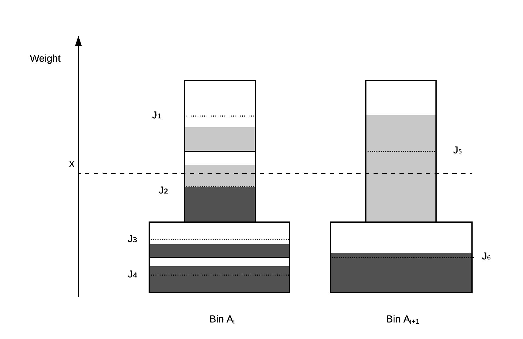
In this figure, each job is described by a rectangular container. The height of the container is the weight of the job, and its area is $2^{j+1}$ for bin $A_{j}$. The area of the gray rectangles inside each container represent the volume of the job. The container is separated into two halves by a dotted line.

The jobs are arranged in the bins according to $\prec$, with $J_{4}\prec J_{3}\prec J_{2}\prec J_{1}$ and $J_{6}\prec J_{5}$. $\beta(J,t)$ is the height of $J$ in this figure - for example, $\beta(J_{2},t)=w(J_{3})+w(J_{4})$.

The volume under $x$ is illustrated by a darker gray. For example:

• For $J_{3}$ we have $\beta(J_{3},t)+w(J_{3})=w(J_{4})+w(J_{3})\leq x$ and therefore $\gamma_{J_{3}}(x,t)=p_{t}(J_{3})$.

• For $J_{2}$ we have that $\beta(J_{2},t)+\frac{w(J_{2})}{2}\leq x<\beta(J_{2},t)+w(J_{2})$ giving that $\gamma_{J_{2}}(x,t)$ is the area of $J_{2}$ under the dotted line. In other words, it is $\min(2^{i},p_{t}(J_{2}))=2^{i}$.

• For $J_{5}$ we have that $\beta(J_{5},t)+\frac{w(J_{5})}{2}>x$, which yields $\gamma_{J_{5}}(x,t)=0$.

As for processing, note that the algorithm will process bin $A_{i+1}$ and not $A_{i}$, though their weights are equal. This is since $J_{1}$ adds only $\frac{w(J_{1})}{2}$ to $\mathscr{W}_{A_{i}}(t)$, because $J_{1}$’s volume is under its dotted line. Since the volume of $J_{5}$ is above $J_{5}$’s dotted line, it adds its full weight, $w(J_{5})$, to $\mathscr{W}_{A_{i+1}}(t)$.