The Axial Zone of Avoidance in the Globular Cluster System and the Distance to the Galactic Center

Abstract—We have checked the existence of a zone of avoidance oriented along the Galactic rotation axis in the globular cluster (GC) system of the Galaxy and performed a parametrization of this zone in the axisymmetric approximation. The possibility of the presence of such a structure in the shape of a double cone has previously been discussed in the literature. We show that an unambiguous conclusion about the existence of an axial zone of avoidance and its parameters cannot be reached based on the maximization of the formal cone of avoidance due to the discreteness of the GC system. The ambiguity allows the construction of the representation of voids in the GC system by a set of largest-radius meridional cylindrical voids to be overcome. As a result of our structural study of this set for northern and southern GCs independently, we have managed to identify ordered, vertically connected axial zones of avoidance with similar characteristics. Our mapping of the combined axial zone of avoidance in the separate and joint analyses of the northern and southern voids shows that this structure is traceable at $|Z|\mathrel{\hbox{\hbox to0.0pt{\hbox{\lower 4.0pt\hbox{$\sim$}}\hss}\hbox{$>$}}}1$ kpc, it is similar in shape to a double cone whose axis crosses the region of greatest GC number density, and the southern cavity of the zone has a less regular shape than the northern one. By modeling the distribution of Galactocentric latitudes for GCs, we have determined the half-angle of the cone of avoidance $\alpha_{0}={15\hbox{$.\!\!^{\circ}$}0}^{+2\hbox{$.\!\!^{\circ}$}1}_{-4\hbox{$.\!\!^{\circ}$}1}$ and the distance to the Galactic center ${R_{0}}=7.{\color[rgb]{0,0,0}3}\pm 0.{\color[rgb]{0,0,0}5}$ kpc (in the scale of the Harris (1996) catalog, the 2010 version) as the distance from the Sun to the point of intersection of the cone axis with the center–anticenter line. A correction to the calibration of the GC distance scale obtained in the same version of the Harris catalog from Galactic objects leads to an estimate of ${R_{0}}=7.{\color[rgb]{0,0,0}2}\pm 0.{\color[rgb]{0,0,0}5}\bigr{|}_{\text{\color[rgb]{0,0,0}stat}}\pm 0.{\color[rgb]{0,0,0}3}\bigr{|}_{\text{\color[rgb]{0,0,0}calib}}~{}\text{kpc}$. The systematic error in $R_{0}$ due to the observational incompleteness of GCs for this method is insignificant. The probability that the zone of avoidance at the characteristics found is random in nature is ${\leq}2\%$. We have revealed evidence for the elongation of the zone of avoidance in the direction orthogonal to the center–anticenter axis, which, just as the north–south difference in this zone, may be attributable to the influence of the Magellanic Clouds. The detectability of similar zones of avoidance in the GC systems of external galaxies is discussed.

Keywords: globular cluster system, spatial distribution, structure, solar Galactocentric distance, Galaxy (Milky Way).

1 INTRODUCTION

Globular clusters (GCs) are traditionally used to study the structure, kinematics, dynamics, chemical evolution, and other properties of the Galactic halo and the Galaxy as a whole (see, e.g., Borkova and Marsakov 2000; Harris 2001; Ashman and Zepf 2008; Loktin and Marsakov 2009). In particular, following the pioneering paper by Shapley (1918), the solar Galactocentric distance ($R_{0}$) is determined from GCs, with GCs having been the most popular type of objects for this purpose until recently. As a rule, one or another modification of Shapley’s method was applied to estimate $R_{0}$ from GCs; it consists in finding the distance to the centroid of the spatial distribution of GCs, i.e., to the geometric center or the point of greatest density of the GC system (for recent implementations see Maciel 1993; Rastorguev et al. 1994; Harris 2001; Bica et al. 2006). However, the unfolded discussion of the observational selection of GCs attributable to extinction and leading to an underestimation of $R_{0}$ in the classical version of Shapley’s method (see the reviews by Reid (1993), Nikiforov (2003), and the references in Table 8 of this paper) has stimulated a search for other, apart from a central concentration, peculiarities of the spatial distribution of GCs that are capable of giving constraints on $R_{0}$ without any significant systematic bias due to the selection effect. For example, Sasaki and Ishizawa (1978) proposed to use the cone of avoidance (COA) in the GC system, by which a drop in the number density or a complete absence of GCs in the double cone whose axis is orthogonal to the Galactic plane and whose vertex lies at the Galactic center is meant, to determine $R_{0}$ .

Wright and Innanen (1972b) were the first to draw attention to the “apparent dearth of GCs in a ${\sim}15\hbox{${}^{\circ}$}$ ‘cone of avoidance’ centered on a Galactic nucleus” in the GC distribution on the $XZ$ plane by alluding to Fig. 3 in the review of Oort (1965) as an illustration. Here, $X$ is the axis passing through the Sun and the Galactic center, $Z$ is the axis orthogonal to the Galactic plane, and the Sun is at the coordinate origin. Wright and Innanen (1972b) assumed a connection between the presence of COA and the following theoretical result. Wright and Innanen (1972a) investigated the collapse of a massless, nonrotating gas spheroid around a massive point nucleus without any gas pressure. They showed analytically that the gas envelope attained an “infinity-sign” shape in a meridional section as a result of the collapse (at the instant of the central singularity). At the same time, the authors pointed out that for a rotating initial spheroid the result should change insignificantly, in particular, because the angular momentum per unit mass of a real protogalaxy should be small near the rotation axis. Wright and Innanen (1972b) associated the deficit of gas arising from the collapse along the minor axis of the spheroid with the COA in the Galactic GC system. However, the conclusion about the existence of the COA itself was qualitative, being apparently based only on the visual impression from the pattern of the GC distribution in projection onto the $XZ$ plane. The brief article by Wright and Innanen (1972b) contains no mention of any statistical analysis of the GC distribution, any estimation of its parameters.

Based on the results and ideas of Wright and Innanen (1972a, 1972b) but without touching on the question of whether the existence of COA in the Galactic GC system was real, Sasaki and Ishizawa (1978) considered the possible dynamical mechanisms for the formation of this structure. Sasaki and Ishizawa (1978) numerically simulated the evolution of an initially spherically symmetric GC system in the Galactic field and showed that the instability of orbits with a low angular momentum and the tidal disruption of GCs as a result of their passage near the Galactic nucleus could collectively give rise to COA in the GC system in a time of ${\sim}10$ Gyr; the peripheral regions of the COA are “cleaned” of GCs faster. In the same paper the COA in the sense of a complete absence of GCs in it was first used to determine the distance to the Galactic center by which the point of intersection of the COA axis with the $X$ axis was meant. As a result, Sasaki and Ishizawa (1978) derived an estimate of $R_{0}=9.2\pm 1.3$ kpc from the COA and an estimate of the COA half-angle $\alpha_{0}=14\hbox{$.\!\!^{\circ}$}3\pm 2\hbox{$.\!\!^{\circ}$}8$.

We have failed to find more recent papers devoted directly to GCs in which the COA would be investigated or its existence would be questioned or it would simply be mentioned, although the interest in this structure, if it is real, and its allowance in solving various problems would seem obvious. At the same time, the $R_{0}$ estimate obtained by Sasaki and Ishizawa (1978) from the COA has been traditionally included in reviews on the problem of $R_{0}$ determination up until now (de Vaucouleurs 1983; Kerr and Lynden-Bell 1986; Reid 1989, 1993; Surdin 1999; Francis and Anderson 2014); it was taken into account when deriving the mean (“best”) value $\langle R_{0}\rangle_{\text{best}}$ in many of its calculations (de Vaucouleurs 1983; Kerr and Lynden-Bell 1986; Reid 1989, 1993; Surdin 1999; Nikiforov 2004; Nikiforov and Smirnova 2013). In comparison with the present-day measurements of this parameter, $\langle R_{0}\rangle_{\text{best}}=(7.8$–$8.25)\pm(0.1$–$0.5)$ kpc (Reid 1993; Nikiforov 2004; Avedisova 2005; Genzel et al. 2010; Foster and Cooper 2010; Nikiforov and Smirnova 2013; Bland-Hawthorn and Gerhard 2016), the individual $R_{0}$ estimates published since 2000 have point values no greater than 8.9 kpc (Francis and Anderson 2014; Bland-Hawthorn and Gerhard 2016), $R_{0}=9.2$ kpc deduced by Sasaki and Ishizawa (1978) seems overestimated.

Below we discuss the possible causes of this discrepancy. However, the main goal of this paper is to check the very fact of the existence of an axial zone of avoidance in the Galactic GC system and, in the case of an affirmative answer to this question, to clarify the characteristic features of the geometry of this zone and to redetermine $R_{0}$ using this spatial structure from the currently available data on GCs.

It should be noted that the principle of finding $R_{0}$ from the COA itself proposed by Sasaki and Ishizawa (1978), irrespective of the systematics of its first realization, can be promising. Since the position of the COA is determined mainly by the clusters at large $|Z|$ (Sasaki and Ishizawa 1978), i.e., at high $|b|$, the selection effect must have virtually no influence on the result; the problem of extinction correction when determining the distances to these GCs is also less acute for them. Therefore, the corresponding systematic biases of the $R_{0}$ estimate are expected to be smaller in the case of using the COA as a key feature of the spatial distribution of GCs than in the case of relying on the GC centroid in Shapley’s method.

2 DATA ON GLOBULAR CLUSTERS

As the database we took the 2010 version of the catalog by Harris (1996) below referred to as H10. The heliocentric distances calculated using the scale

$$M_{V}(\text{HB})=0.16\,\text{[Fe/H]}+0.84,$$ (1)

adopted by Harris based on his own calibration from new data are given for all 157 clusters of the catalog. Here, $M_{V}(\text{HB})$ is the mean absolute $V$ magnitude of the horizontal branch, and [Fe/H] is the metallicity.

The [Fe/H] estimates given in H10 for 152 GCs were used in this paper only to separate the metal-rich and metal-poor cluster subsystems. We adopted the boundary metallicity [Fe/H] = −0.8 (Nikiforov and Smirnova 2013).

3 THE METHOD OF MAXIMIZING THE FORMAL
CONE OF AVOIDANCE

The estimate of $R_{0}=9.2\pm 1.3$ kpc deduced by Sasaki and Ishizawa (1978) was obtained for the catalog of distances with the calibration $M_{V}({\rm HB})=0{{}^{m}\!\!\!.\,}5$ that is brighter than the present-day ones, i.e., gives a longer scale. Rescaling the estimate to calibration (1) gives $R_{0}=8.7\pm 1.2$ kpc for $\text{[Fe/H]}=-1.3$, the mean metallicity for all GCs, and $R_{0}=8.8\pm 1.2$ kpc for $\text{[Fe/H]}=-1.5$, the mean metallicity for metal-poor GCs (Nikiforov and Smirnova 2013), which largely determine the COA. Clearly, these values of $R_{0}$ do not contradict the present-day estimates, although they are near the edge of their range. However, Sasaki and Ishizawa (1978) provided another estimate from the COA, $R_{0}=9.4\pm 1.2$ kpc, based on one of the early versions of the catalog by Harris with more accurate GC distances and the calibration $M_{V}({\rm HB})=0{{}^{m}\!\!\!.\,}6$. Rescaling to calibration (1) barely changes this estimate: $R_{0}=9.3\pm 1.2$ and $R_{0}=9.4\pm 1.2$ kpc for $\text{[Fe/H]}=-1.3$ and $-1.5$, respectively. The latter values suggest that, on the whole, the procedure by Sasaki and Ishizawa (1978) leads to overestimates of $R_{0}$ from the COA; the overestimation cannot be explained by the evolution of the GC distance scale calibration.

Sasaki and Ishizawa (1978) used the natural principle of maximizing the COA opening angle as the basis for their analysis: the value of $R_{0}$ at which this angle turns out to be largest is taken to be the “true” one. Obviously, the COA determined in this way in nondegenerate cases is specified by only two GCs (for an explanation see below, after Eq. (3)). Sasaki and Ishizawa (1978) did not apply this procedure to the original catalogs of distances, apparently because the optimal value of $R_{0}$ in such a case is based only on two distance estimates having some uncertainties. Instead, they maximized the COA for each of the 300 pseudo-random GC catalogs obtained by varying the distances moduli of GCs according to a normal law with a mean corresponding to the cataloged distance and a standard deviation of ${0^{m}\!\!\!.\,5}$ or ${0^{m}\!\!\!.\,3}$ for different original catalogs. The trial values of $R_{0}$ were taken in the range from 6 to 12 kpc. The optimal values of $R_{0}$ found for each generated catalog were then averaged.

To find out what the systematics of this procedure could be, let us consider the dependence of the largest (in absolute value) Galactocentric latitude of GCs, $\varphi_{0}\equiv\pi/2-\alpha_{0}=\max|\varphi|$, on the adopted $R_{0}$ derived from the H10 data (Fig. 1a). Here, the Galactocentric latitude of an individual GC, $\varphi$, at a given $R_{0}$ is defined by the expression

$$\varphi=\arctan{\frac{Z}{R}}\,,$$ (2)

where $Z$ is the GC height above the Galactic plane, and $R$ is the distance from the GC to the Galactic rotation axis (Galactoaxial distance). In turn,

$$Z=r\sin{b},\qquad R=\sqrt{R^{2}_{0}+r^{2}\cos^{2}b-2R_{0}r\cos{l}\cos{b}},$$ (3)

where $r$ is the heliocentric distance, $l$ and $b$ are the Galactic longitude and latitude of the GC. Equations (2) and (3) show that the function $|\varphi|(R_{0})$ for an individual GC has a (single) maximum at minimum $R$ (i.e., at $R_{0}$ at which the formal radius vector drawn to the GC is orthogonal to the $X$ axis), while this function has no minima. Each segment of the function $\varphi_{0}(R_{0})$ in Fig. 1a that has a continuous derivative for some interval of $R_{0}$ is a segment of the dependence $|\varphi|(R_{0})$ for the GC that has the largest $|\varphi|$, i.e., determines $\varphi_{0}$ , in this interval of $R_{0}$ . Hence a local minimum of the function $\varphi_{0}(R_{0})$ can emerge only if at some value of the argument +$R_{0}=R_{0}^{*}$ the decreasing segment of the function $|\varphi|(R_{0})$ for some GC determining $\varphi_{0}$ at $R_{0}<R_{0}^{*}$ will obtain a value equal to the value of the increasing segment of the function $|\varphi|(R_{0})$ for another GC determining $\varphi_{0}$ at $R_{0}>R_{0}^{*}$ . Thus, the position of each minimum of $|\varphi|(R_{0})$, including the global one, is determined by the data on only two GCs, i.e., the formal maximization of the COA gives a solution that eventually “relies” on the pair of GCs selected through this procedure.

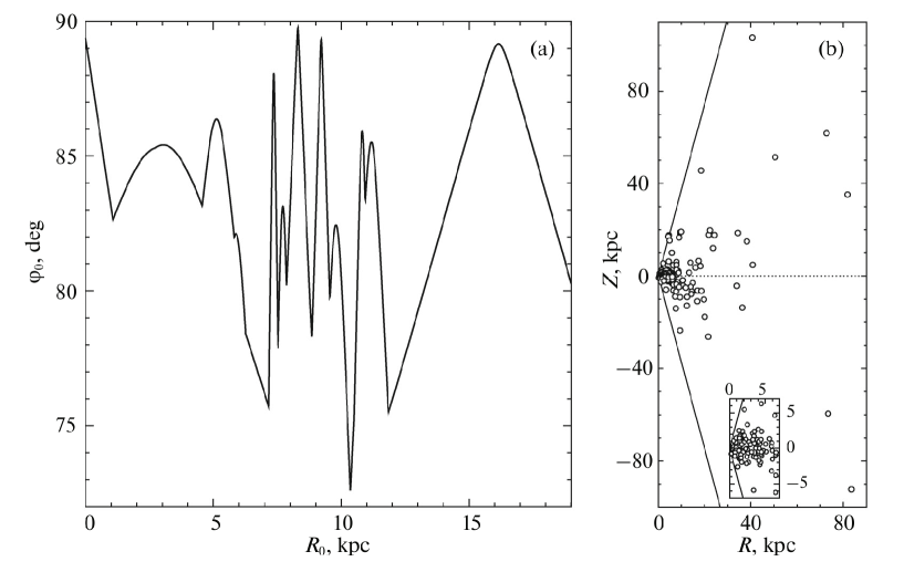
Fig. 1: (a) Largest (in absolute value) Galactocentric latitude of GCs, $\varphi_{0}\equiv\pi/2-\alpha_{0}$, versus adopted $R_{0}$ . (b) The spatial distribution of GCs in coordinates $(R,Z)$, where $R$ is the Galactoaxial distance, $Z$ is the height above the Galactic plane, for one of the minima of the dependence $\varphi_{0}(R_{0})$ ($R_{0}=7.16$ kpc); the oblique straight lines correspond to the boundaries of the axial cone with a half-angle $\alpha_{0}=15^{\circ}$.

The COA must lead to a minimum of depth ${\approx}\alpha_{0}$ in the plot of the dependence $\varphi_{0}(R_{0})$. Figure 1a shows that this dependence actually has three deep minima (at $R_{0}=7.16$, $10.36$, and $11.85$ kpc) with comparable opening angles $\alpha_{0}\mathrel{\hbox{\hbox to0.0pt{\hbox{\lower 4.0pt\hbox{$\sim$}}\hss}\hbox{$>$}}}15^{\circ}$ and several shallower ones. Obviously, the numerous local minima are attributable to the discreteness of the GC system, which increases with distance from the Galactic center, especially in the post-central region where the undetectability of GCs increases sharply (Nikiforov and Smirnova 2013). The fact that two of the three deepest minima occur at $R_{0}>10$ kpc provides evidence for the latter effect. Strictly speaking, based only on this dependence, we cannot understand which of the minima corresponds to the real COA and which are “spurious.” The GC distribution on the $RZ$ plane with a characteristic conical region of avoidance along the $Z$ axis shown in Fig. 1b for the minimum at $R_{0}=7.16$ kpc turns out to be similar for the other two deep minima as well.

This ambiguity is not removed by varying the distances to clusters. For each pseudo-random catalog Sasaki and Ishizawa (1978) chose $R_{0}$ that corresponded to the deepest formal minimum of $\varphi_{0}(R_{0})$ without any attempt to distinguish the axial (central) minimum from the off-axis (peripheral) ones. The depth of the minima also varies when varying the distances, and if there are two or more comparable minima, then sometimes one, sometimes another can become the deepest of them. Consequently, averaging the formal solutions over all model catalogs either is actually averaging the values of $R_{0}$ for the deepest minima of the initial dependence $\varphi_{0}(R_{0})$ or gives the average position of one (deepest) minimum, which may turn out to be an off-axis one. In the first case, the mean $R_{0}$ is found to be, in general, shifted, while its variance more likely reflects the scatter in the positions of the deep minima than the influence of the errors in the distances on the position of the deepest of them. Indeed, a formal averaging of the positions of three minima in Fig. 1a gives $R_{0}=9.8\pm 1.4$ kpc, a value close to the point estimates and uncertainties in the results from Sasaki and Ishizawa (1978). Even if the second case is realized, the global minimum of $\varphi_{0}(R_{0})$ will very likely to be an off-axis one. For the original H10 data it turns out to be such, leading to an even larger $R_{0}=10.4$ kpc (Fig. 1a). Note that the dependences $\varphi_{0}(R_{0})$ constructed by us from earlier GC catalogs for various samples are similar in basic features to the dependence in Fig. 1a: there were a total of two or three comparable deep minima the deepest of which, as a rule, was at $R_{0}\sim 10$ kpc; the structure of the middle part of the dependence only became more complicated with time due to the appearance of a larger number of central GCs in the catalogs. Sasaki and Ishizawa (1978) did not provide the curve $\varphi_{0}(R_{0})$.

Since the discreteness of the GC system behind the Galactic center is higher because of the selection effect (Nikiforov and Smirnova 2013), the occurrence probability of deep off-axis minima is also higher there (Fig. 1a). This explains why the values obtained by Sasaki and Ishizawa (1978) were overestimated.

Thus, applying the method of maximizing the formal COA generally leads to an incorrect result, irrespective of whether the GC distances are varied or not. Modeling the distribution of Galactocentric latitudes for GCs whereby the $R_{0}$ estimate is determined by the spatial distribution of all GCs from the sample can be an alternative. The dependences $|\varphi|(R_{0})$ only for two GCs are eventually used in maximizing the COA.

However, before we turn to this modeling, the very fact of the existence of a region of avoidance should be checked, because, strictly speaking, the mere presence of deep minima in the plot of $\varphi_{0}(R_{0})$ does not prove this fact: all these minima can be off-axis ones attributable to the discreteness of the GC system. If the existence of a region of avoidance will be confirmed, then it is also necessary to establish the main geometric properties of this region.

4 MAPPING THE AXIAL ZONE OF AVOIDANCE
IN THE GLOBULAR CLUSTER SYSTEM

4.1 Representation of Voids by a Set of Meridional Cylindrical Voids

To study the regions of avoidance in the GC system oriented along the $Z$ axis, let us partition the entire space into layers whose boundaries are parallel to the Galactic plane. We will begin the partition in the northward and southward directions from the Galactic plane ($Z=0$ kpc) and will select the boundaries of the layers in such a way that the number of GCs in each layer is no smaller than ten. As a result of the partition, we obtained 14 $Z$ layers and, accordingly, GC samples. Following the principle of maximizing the region of avoidance (Sasaki and Ishizawa 1978), we will search for the largest voids in each layer along the local (passing through the Sun) meridional plane of the Galaxy. For this purpose, we constructed the dependence ${\rho}(X)$ for each $Z$ layer, where $\rho$ is the distance from a point on the $X$ axis ($X$ is the coordinate of the point) to the nearest GC projection onto the $XY$ plane (Galactic plane); the $Y$ axis points in the direction of Galactic rotation. In this dependence we found local maxima ${\rho}_{\text{c}}\equiv{\rho}(X_{\text{c}})$, each of which specifies the locally largest (in volume) cylindrical region of avoidance (in which there are no GCs) with radius ${\rho}_{\text{c}}$ and axis coordinate $X_{\text{c}}$ (here, “c” stands for cylinder). Below we will call such regions cylindrical voids (CVs). Here, we restrict our analysis only to the meridional CVs whose axes lie in the local meridional plane of the Galaxy. A set of CVs was found for each $Z$ layer. As an example, Fig. 2 presents the dependences ${\rho}_{\text{c}}(X)$ for the southern $Z$ layers, while Fig. 3 shows the projections of the CVs found for these layers onto the $XY$ plane. Also, the open and filled circles of the same size in Fig. 3 indicate, respectively, the GCs determining the CVs and the remaining GCs that fell into the $Z$ layer; the small filled circles mark the positions of the CV axes.

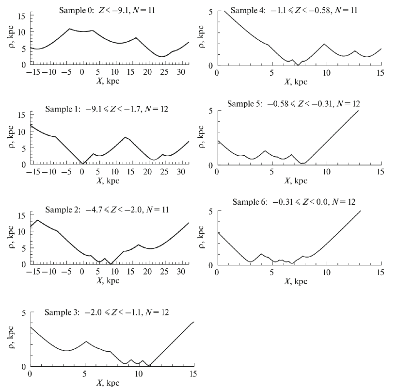
Fig. 2: Distance $\rho$ from a point on the $X$ axis to the nearest GC projection onto the Galactic plane versus coordinate $X$ of this point for the southern $Z$ layers. The origin of the $X$ axis corresponds to the position of the Sun.

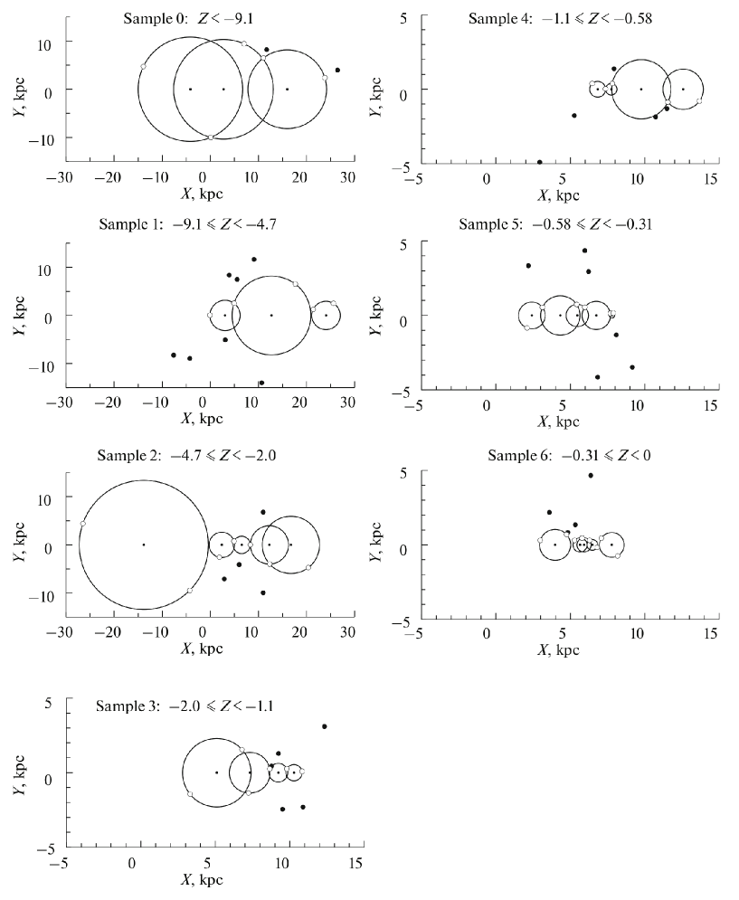
Fig. 3: Cylindrical voids found in projection onto the Galactic plane ($XY$) for the southern $Z$ layers. The open circles are the GCs determining the voids; the large filled circles are the remaining clusters falling into a $Z$ layer; the small filled circles are the positions of the void axes. The Sun is at point $(X,Y)=(0,0)$.

The projection of the constructed CV system onto the $XZ$ plane allows the void distribution pattern as a whole to be imagined. Let us introduce new terms and designations. As can be seen from Fig. 3, CVs can intersect. If (two or more) voids intersect, i.e., if they are nonisolated, then the single combined void formed by them is considered. The vertical boundaries of the latter in projection onto the $XZ$ plane are the leftmost and rightmost boundaries of the CVs constituting it; they will be depicted by solid lines. We will designate the edges of the CV intersections by long dashes and the boundaries of the nonisolated CVs that fell into the combined voids by short dashes. Figure 4 (lower panel) gives an example of the projection of one of the $Z$ layers onto the $XZ$ plane. The upper and middle panels of Fig. 4 for the same $Z$ layer show the dependence ${\rho}(X)$ and the CV projections onto the $XY$ plane, respectively. On the two lower panels of Fig. 4, just as in Fig. 3, the open and filled circles depict, respectively, the GCs determining the CVs and the remaining GCs that fell into the $Z$ layer.

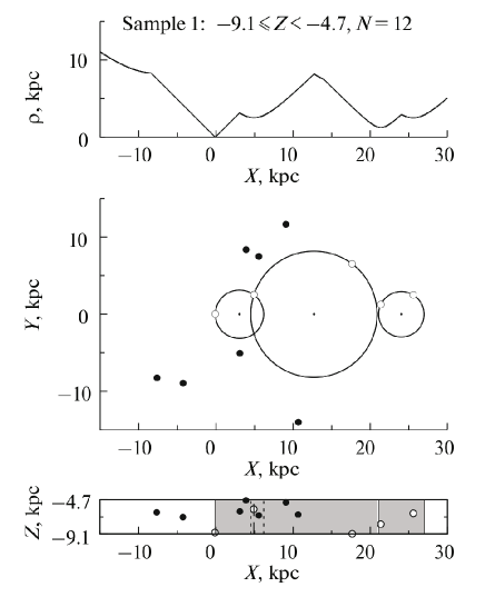
Fig. 4: Finding the locally maximal CVs and constructing their scheme for one of the $Z$ layers as an example. The upper panel: the function ${\rho}(X)$ whose local maxima, ${\rho}_{\text{c}}\equiv{\rho}(X_{\text{c}})$, determine the axis coordinates ($X_{\text{c}}$) and radii (${\rho}_{\text{c}}$) of the voids. The middle panel: the projection of the voids onto the $XY$ plane. The lower panel: the projection of the $Z$ layer onto the $XZ$ plane. The gray shading depicts the void cavities. The designations for GCs are the same as those in Fig. 3.

Using the introduced designations, let us construct a general scheme of the CV distribution in space. Figure 5 shows the projection of the entire set of CVs identified in 14 $Z$ layers onto the $XZ$ plane. Since the height of the $Z$ layers increases dramatically with $|Z|$ due to the rapid drop in the number density of clusters, we will use a logarithmic scale for the $Z$ coordinate in this and subsequent figures presenting the zone of avoidance: $\pm\log(1+|Z|)$. For comparison, Fig. 5 plots the contours of the presumed COAs (the curves in the adopted coordinates) with half-angles $\alpha_{0}=14^{\circ}$ and $18^{\circ}$ corresponding to the scatter of estimates for this parameter in Sasaki and Ishizawa (1978); here, $R_{0}=7.9$ kpc (Nikiforov 2004; Nikiforov and Smirnova 2013).

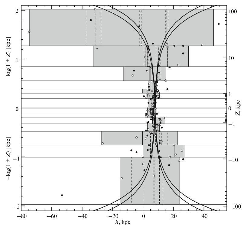
Fig. 5: Scheme of the entire set of CVs identified in the GC system. The void cavities are highlighted by the gray shading. The vertical lines have the same meaning as those on the lower panel of Fig. 4 (see the text). The curves depict the contours of the axial cones with $\alpha_{0}=14^{\circ}$ and $18^{\circ}$ for $R_{0}=7.9$ kpc. The designations for GCs are the same as those in Fig. 3.

4.2 Identification of the Axial Zone of Avoidance through a Separate Analysis
of the Northern and Southern Voids

Figure 5 shows that the voids form a cone-shaped structure, but wider than the presumed COA. The latter is not surprising, because many of the CVs found are, obviously, only formal constructions and do not belong to the sought-for axial structure due to the discreteness of the GC distribution. Therefore, from the entire set of CVs we will separate out the subsets of voids each of which forms a vertically connected structure. As a criterion for constructing such structures and a subset of CVs we will take the existence of an interval (with zero length inclusive) on the $X$ axis in which all of the rays with the origins on this axis directed along the $Z$ axis in the northward or southward direction pass, respectively, all northern or southern $Z$ layers only through the cavities of the voids of this subset without anywhere crossing the region of the $Z$ layer where there is no void. We will call this algorithm a semi-through one. Thus, in this step we consider the northern and southern voids separately. If the axial zone of avoidance in the GC system is real, then it must be detected in the northern and southern halves of the Galaxy independently and with similar characteristics.

As a result of the above analysis, we found five northern and three southern vertically connected subsets of CVs. Let us identify those CVs that are common to all northern or all southern subsets. Obviously, we can talk about the existence of an axial zone of avoidance only if such common CVs will be found and will constitute an ordered structure.

The scheme of the revealed common voids (Fig. 6) shows that both take place. The common CVs form a generally ordered axial zone of avoidance similar in shape to a double conical surface. Below we will call these voids axial. As can be seen from Fig. 6, no significant deviations from the conical shape are observed; the dispersion of the void boundaries relative to this model, but without any obvious systematic bias, is higher only in the southern part of the Galaxy. There is no evidence for any serious inclination of the axis of the zone of avoidance to the Galactic plane either; otherwise we would obtain a noticeably asymmetric picture of the void boundaries. It is obvious that, for example, the cylindrical model for the zone of avoidance is unsuitable, because the radii of the axial CVs, on the whole, increase with $|Z|$ (Fig. 6).

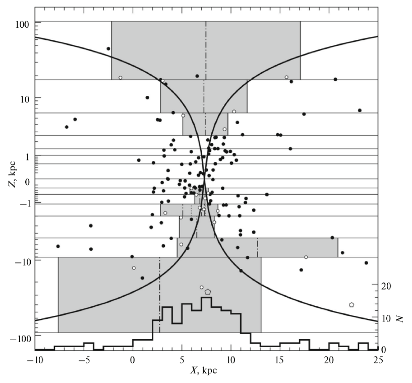
Fig. 6: Axial zone of avoidance in the GC system from the results of our separate analysis of the southern and northern voids. The shading designates the axial voids; the dash–dotted lines indicate their axes. The solid curves mark the contour of the axial cone with $\alpha_{0}=15\hbox{$.\!\!^{\circ}$}0$ for $R_{0}=7.3$ kpc (see Subsection 5.3). The histogram is the GC distribution along the $X$ axis. The pentagons are the LMC and SMC galaxies. The remaining designations are the same as those in Fig. 5.

Comparison with the GC distribution along the $X$ axis (the histogram in Fig. 6) shows that the positions of the axes of both northern and southern parts of the revealed zone of avoidance are close to the maximum of the GC number density at $X\approx 7$–$8$ kpc. The opening angle of the zone of avoidance roughly corresponds to expectations (Fig. 6).

The axial structure is not unambiguously identified in the layers at small $|Z|$. This is consistent with the results of numerical experiments by Sasaki and Ishizawa (1978), showing that the COA is “cleaned” of GCs primarily in the peripheral regions, while near the Galactic center GCs must be preserved within the formal COA even on time scales of ${\sim}20$ Gyr.

The axis coordinates ($X_{\text{c}}$) of the identified axial CVs were processed as a series of equally accurate measurements and as a series of measurements with weights $p=1/\rho_{\text{c}}$ , where $\rho_{\text{c}}$ is the CV radius. The choice between these two cases is ambiguous, because, on the one hand, $X_{\text{c}}$ is determined more accurately at a small void radius and, on the other hand, the axial zone itself is mainly determined by the voids at larger $|Z|$, where the void radii are also larger. We considered the entire set of axial voids as well the northern and southern voids separately. The processing results are presented in Tables 1 and 2. The notation: $N$ is the number of voids, $\overline{X_{\text{c}}}$ is the mean value of $X_{\text{c}}$, ${\sigma}_{X_{\text{c}}}$ is the standard deviation of $X_{\text{c}}$ from $\overline{X_{\text{c}}}$, $\sigma_{0,X_{\text{c}}}$ is the mean error per unit weight, and ${{\sigma^{\prime}}}_{{X}_{\text{c}}}$ is the weighted standard deviation of $X_{\text{c}}$ from $\overline{X_{\text{c}}}$ . For the adopted mean position of the axis $\overline{X_{\text{c}}}$ in each axial void the formal COA is specified by one of the two void-forming GCs that has the largest absolute value of the Galactocentric latitude, $\varphi_{\text{m}}\equiv\max(|\varphi_{1}|,|\varphi_{2}|)$. Tables 1 and 2 give the statistics $\overline{\varphi_{\text{m}}}$, ${\sigma}_{\varphi_{\text{m}}}$, and $\varphi_{0}$ , i.e., the arithmetic mean, standard deviation, and maximum value of $\varphi_{\text{m}}$ , respectively.

Tables 1 and 2 show that the values of $\overline{X_{\text{c}}}$ for all samples and averagings differ only within the error limits. At the same time, $\overline{X_{\text{c}}}\approx 7$ kpc in all cases, except one case (Table 1, $Z<0^{\circ}$) for which the uncertainty in $\overline{X_{\text{c}}}$ is great. The values of $\overline{X_{\text{c}}}\approx 7$ kpc are close to one of the minima in Fig. 1a ($R_{0}=7.16$ kpc); it apparently corresponds, to a first approximation, to the position of the COA axis; the remaining minima in this figure are off-axis ones. The values of $\varphi_{0}$ for GCs also turn out to be similar.

There is a north–south difference in $\overline{\varphi_{\text{m}}}$ . There are more void-forming GCs with relatively small $|\varphi|$ in the southern part of the axial zone of avoidance; besides, in the layer $-2.0\text{ kpc}\leq Z<-1.1$ kpc, i.e., relatively close to the Galactic plane, we found two nonisolated axial voids forming an extended structure along the $X$ axis (Fig. 6). This is responsible for the smaller $\overline{\varphi_{\text{m}}}$ for $Z<0$ kpc. For the northern part of the zone the uncertainty in $\overline{X_{\text{c}}}$, along with all other dispersion characteristics, turn out to be noticeably smaller than those for the southern one (Tables 1 and 2), which reflects a more regular pattern of the northern cavity of the zone of avoidance (Fig. 6).

On the whole, the results obtained argue for the existence of a zone of avoidance for GCs similar in shape to a double cone along the Galactic axis (outside the small central region). The northern and southern cavities of the COA manifest themselves independently and with similar parameters ($\overline{X_{\text{c}}}$, $\varphi_{0}$). The latter gives us grounds to perform a joint analysis of the northern and southern CVs in the next subsection to increase the identifiability of axial voids.

4.3 Identification of the Axial Zone of Avoidance by Analyzing the Entire Set of Voids

Let us return to the complete set of CVs constructed in Subsection 4.1. Let us separate out the subsets of voids from it each of which forms a through vertically connected structure. Thus, in contrast to the semi-through algorithm of Subsection 4.2, as a criterion for the separation of a CV subset we will take the existence of an interval (with zero length inclusive) on the $X$ axis in which all of the straight lines crossing this axis and lying parallel to the $Z$ axis pass all northern and southern $Z$ layers only through the cavities of the voids of this subset without anywhere crossing the region of the Z layer where there is no void. We will call this algorithm a through one.

As a result of this analysis, we found 22 different combinations of voids constituting through vertically connected structures. The identification of CVs common to all these combinations gives eight axial voids (four northern and four southern ones). The scheme of the latter is presented in Fig. 7; the characteristics of the axial zone formed by them are given in Tables 3 and 4, where the designations are the same as those in Tables 1 and 2.

Fig. 7: Axial zone of avoidance in the GC system from the results of our analysis of the entire set of voids. The designations are the same as those in Fig. 6.

The new results turned out to be generally similar to those based on the semi-through algorithm. However, the zone of avoidance constructed using the through algorithm is more symmetric, both relative to the Galactic plane and relative to the mean axis, and more ordered (cf. Figs. 6 and 7). In particular, this manifests itself in the facts that, in contrast to the results of the previous subsection, the number of northern and southern axial voids turned out to be the same, there are no nonisolated CVs among them, the $Z$ boundaries of unambiguous identification of the axial zone closest to the Galactic plane are similar in absolute value for the northern and southern cavities of the zone, respectively, $Z_{\text{lim}}=+1.435$ и $-1.1$ kpc ($Z_{\text{lim}}=+2.6$ and $-0.31$ kpc were obtained in Subsection 4.2), the north–south difference in $\overline{\varphi_{\text{m}}}$ and ${\sigma}_{\varphi_{\text{m}}}$ decreased dramatically, the difference between the formal angular boundaries of $\varphi_{0}$ for the northern and southern COAs was slightly reduced. In addition, the positions of the mean axis of the zone of avoidance in all cases turned out to be very close ($7.12\leq\overline{X_{\text{c}}}\leq 7.3$ kpc), the scatter of $\overline{\varphi_{\text{m}}}$ in different cases became much smaller ($60^{\circ}$–$68^{\circ}$ versus $48^{\circ}$–$70^{\circ}$ in Subsection 4.2), the standard deviation ${\sigma}_{\varphi_{\text{m}}}$ was generally also reduced (cf. Tables 3, 4 and Tables 1, 2).

Thus, the through algorithm identifies a zone of avoidance with a more regular structure closer to a conical one. Although the main north–south differences noted in the previous subsection turn out to be smaller, they do not disappear completely. They apparently reflect the objective properties of the spatial distribution of Galactic GCs.

Note that in all cases in Tables 3 and 4 the estimates of $\overline{\varphi_{\text{m}}}$ and ${\sigma}_{\varphi_{\text{m}}}$ differ significantly from the mean $\operatorname{\mathsf{M}}\Phi_{\text{m}}=\pi/4=45\hbox{${}^{\circ}$}$ and standard deviation $(\operatorname{\mathsf{D}}\Phi_{\text{m}})^{1/2}=\frac{\sqrt{\pi^{2}-8}}{4}\approx 19\hbox{$.\!\!^{\circ}$}6$, respectively, for a spherically symmetric GC distribution without COA (see Appendix A2). This suggests that the choice of voidforming clusters using the through algorithm is not random and argues for the reality of the voids in the distribution identified by them.

Our results of mapping the zone of avoidance in the Galactic GC system confirm the existence of an axial COA with a half-angle $\alpha_{0}=\pi/2-\varphi_{0}\approx 13^{\circ}$–$15^{\circ}$ for the system as a whole. Note that for all samples of axial voids the formal COA boundary $\varphi_{0}$ turned out to be stable with respect to the algorithm of identifying the zone of avoidance and the method of processing the void axis coordinates $X_{\text{c}}$ (Tables 1–4).

5 MODELING THE DISTRIBUTION OF GALACTOCENTRIC LATITUDES FOR GLOBULAR CLUSTERS

Having confirmed the existence of COA in the GC system, let us return to the problem of using this structure to determine $R_{0}$ under the assumption of an axial symmetry of the GC system by taking the point of intersection of the COA axis with the center–anticenter line as the Galactic center. To overcome the shortcomings of the method of maximizing the formal COA (see Section 3), we will seek $R_{0}$ as a parameter of the model distribution function of Galactocentric latitudes $\varphi$ for GCs. In this approach the $R_{0}$ estimate will be a function of the positions of all clusters from the sample rather than two of them, as in the COA maximization method.

In this case, the results of Section 4.3 may be used as a priori information, but we may dispense with this. The first and second methods suggest modeling the $\varphi$ distribution only for the void-forming GCs and for the complete GC sample without additional data on the COA, respectively. Each method has its advantages and disadvantages. Consider both cases.

5.1 Modeling for the Void-Forming Globular Clusters of the Axial Zone of Avoidance

For the objects that are exactly on the COA surface the minimum (zero value) of the variance of the absolute values of their Galactocentric latitudes, ${\sigma}^{2}_{|\varphi|}$, is reached at a trial $R_{0}$ equal to the true one. If the void-forming GCs identified in Section 4.3 are assumed to be located near the COA surface, then minimizing ${\sigma}^{2}_{|\varphi|}$ for these GCs gives an estimate of $R_{0}$ as a COA parameter. We will then consider the conditional equations written for $N$ void-forming clusters

$${{|\varphi}_{i}}(R_{0})|=\overline{|\varphi|},\quad i=1,\>\ldots,\>N,$$ (4)

where $\overline{|\varphi|}$ is the mean value of $|\varphi|$ at given $R_{0}$ , and the function $\varphi(R_{0})$ is defined by Eqs. (2) and (3), as an overdetermined system of equations and will solve it by the least-squares method for the unknowns $R_{0}$ and $\overline{|\varphi|}$. Here, we actually assume that $|\varphi|$ for these clusters are distributed according to the normal law ${\cal N}(\overline{|\varphi|},{\sigma}^{2}_{|\varphi|})$, $\overline{|\varphi|}<\varphi_{0}$ .

The results of solving system (4) for the complete sample of void-forming GCs as well as for the northern and southern subsamples of these objects are presented in Table 5. The standard errors are given for $\overline{|\varphi|}$ and ${\sigma}_{|\varphi|}$. In the case of a nonlinear parameter $R_{0}$ , we took the projection of the two-dimensional confidence region with a $1\sigma$ confidence level onto the $R_{0}$ axis as the confidence interval (Press et al. 1997). The boundaries of this interval were found as the roots of the equation

$$\varsigma^{2}(R_{0})=\varsigma^{2}_{0}\left(1+{\frac{1}{N_{\text{free}}}}\right),$$ (5)

where

$$\varsigma^{2}_{0}\equiv\min\left[{\sigma}^{2}_{|\varphi|}\left(R_{0},\overline{|\varphi|}\right)\right],\qquad\varsigma^{2}(R_{0})\equiv\min_{R_{0}\,=\>\text{const}}\left[{\sigma}^{2}_{|\varphi|}\left(R_{0},\overline{|\varphi|}\right)\right],$$ (6)

$N_{\text{free}}$ is the number of degrees of freedom (Nikiforov 1999, 2003; Nikiforov and Kazakevich 2009). We will call the dependence $\varsigma^{2}(R_{0})$ the profile of the objective function for the parameter $R_{0}$ .

The solution was found for each of the three GC samples. The error of $R_{0}$ in all three cases turned out to be quite low, despite the very small size of the samples. The difference between the $R_{0}$ estimates based on the northern and southern samples is not revealing due to its low confidence level ($1.4\sigma$) and the small size of the samples. We took the estimate based on the complete sample of void-forming GCs as the final result within this method: $R_{0}={7.29}^{+0.29}_{-0.28}$ kpc. Figure 8a presents the profile of the objective function for the parameter $R_{0}$ for the complete sample. The profile has a local minimum at $R_{0}=9.34$ kpc, but it is shallow and is found at a $3.6\sigma$ (99.97%) confidence level with respect to the global minimum. Thus, the confidence region for the latter remains connected up to this level. The local minimum is attributable to the southern GCs: it is also present and is deeper for the southern sample and is absent for the northern one.

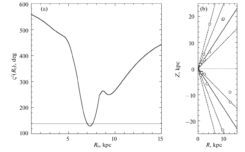
Fig. 8: Solution of system (4) for the complete sample of void-formingGCs. (a) The profile of the objective function ${\sigma}^{2}_{|\varphi|}$ for the parameter $R_{0}$ . The horizontal line marks the $1\sigma$ confidence level. (b) The distribution of GCs from the sample in coordinates $(R,Z)$ for $R_{0}$ = 7.29 kpc. The oblique solid, dashed, and dash–dotted lines correspond to the “model” $\overline{|\varphi|}=57\hbox{$.\!\!^{\circ}$}1$, $\overline{|\varphi|}\pm{\sigma}_{|\varphi|}$ , and the formal COA boundary $\varphi_{0}=75\hbox{$.\!\!^{\circ}$}3$, respectively.

Figure 8b for $R_{0}=7.29$ kpc shows the distribution of GCs from the complete sample in coordinates $(R,Z)$ in comparison with the angular model characteristics. The criterion for excluding the objects with excessive residuals (Nikiforov 2012) does not give grounds to reject some of these clusters even in the most rigorous case ($L^{\prime}=1$).

The estimates of the angular parameters based on the northern and southern samples differ noticeably (Table 5). For example, the difference $\overline{|\varphi|}_{\text{N}}-\overline{|\varphi|}_{\text{S}}=11\hbox{$.\!\!^{\circ}$}4\pm 5\hbox{$.\!\!^{\circ}$}0$ is marginally significant ($2.3\sigma$). Indeed, the distributions of northern and southern GCs in Fig. 8b seem to be somewhat different. However, this does not necessarily imply that the parameters of the northern and southern COA cavities are different, because those southern GCs that are near the void boundaries far from the COA axis make a strong contribution to these differences, while the COA is determined by the clusters near the close boundaries (Figs. 7, 8b). In any case, these results are not an independent confirmation of the north–south difference for the region of avoidance noted in Section 4, being obtained from the same sample of void-forming GCs. We will return to this question after applying the second method, which does not require the selection of clusters and is applicable to their complete sample.

Note that all values of $\overline{|\varphi|}$ in Table 5 exceed considerably and significantly the mean $\operatorname{\mathsf{M}}\Phi=\pi/2-1\approx 32\hbox{$.\!\!^{\circ}$}7$ for a spherically symmetric GC distribution without COA (see Appendix A1).

5.2 Model Distributions of Galactocentric Latitudes

Let us derive the differential distribution law of Galactocentric latitudes $f({\varphi})$ by assuming that the GCs are arranged spherically symmetrically relative to the Galactic center but are completely absent in the COA with a half-angle $\alpha_{0}\equiv\pi/2-\varphi_{0}$ and an axis coincident with the Galactic axis. The GC distribution function in Galactocentric Cartesian coordinates $x$, $y$, and $z$ is then

$${\mathfrak{f}_{1}}(x,y,z)=\mathfrak{f}(R_{\text{g}}),\qquad R_{\text{g}}=\sqrt{x^{2}+y^{2}+z^{2}}=\sqrt{(X-R_{0})^{2}+Y^{2}+Z^{2}}.$$ (7)

Here, $R_{\text{g}}$ is the Galactocentric distance; $X$, $Y$, and $Z$ are the heliocentric Cartesian coordinates. Let us introduce the spherical coordinates $R_{\text{g}}$, $\varphi$, and $\theta$:

$$x=R_{\text{g}}\cos{\varphi}\cos{\theta},\qquad y=R_{\text{g}}\cos{\varphi}\sin{\theta},\qquad z=R_{\text{g}}\sin{\varphi}.$$ (8)

For the distribution function in coordinates $R_{\text{g}}$, $\varphi$, and $\theta$ we then have

$${\mathfrak{f}_{2}}(R_{\text{g}},\varphi,\theta)\,d{R_{\text{g}}}\,d{\varphi}\,d{\theta}={\mathfrak{f}_{1}}(x,y,z)\,d{x}\,d{y}\,d{z}={\mathfrak{f}_{1}}(R_{\text{g}},\varphi,\theta)J\,d{R_{\text{g}}}\,d{\varphi}\,d{\theta},$$ (9)

where $J=R^{2}_{\text{g}}\,\cos{\varphi}$ is the Jacobian (see, e.g., Agekyan 1974). Hence we obtain

$${\mathfrak{f}_{2}}(R_{\text{g}},\varphi,\theta)={\mathfrak{f}}(R_{\text{g}})\,{R^{2}_{\text{g}}}\,\cos{\varphi}.$$ (10)

Integrating (10) over $R_{\text{g}}$ and $\theta$ gives an expression for $f(\varphi)$ to within the normalization constant $c$:

$$f(\varphi)=2\pi cI\cos{\varphi},\qquad I=\int\limits^{a}_{0}{\mathfrak{f}}(R_{\text{g}})\,{R^{2}_{\text{g}}}\,dR_{\text{g}}\,.$$ (11)

The normalization condition

$$1=\int\limits^{\pi/2}_{-\pi/2}{f(\varphi)\,d\varphi}=2\pi cI\int\limits^{\varphi_{0}}_{-\varphi_{0}}{\cos{\varphi}\,d\varphi}=4\pi cI\sin{\varphi_{0}}$$ (12)

defines the constant

$$c=\frac{1}{4\pi I\sin{\varphi_{0}}}\,.$$ (13)

Using (11) and (13), we obtain the sought-for model distribution of angles $\varphi$ for a spherically symmetric GC distribution with an axial COA:

$$f({\varphi})=\left\{\begin{array}[]{ll}\frac{\displaystyle\cos{\varphi}}{\displaystyle 2\sin{\varphi}_{0}}\,,&|{\varphi}|\leq{\varphi}_{0}\,,\\ 0,&|{\varphi}|>{\varphi}_{0}\,.\end{array}\right.$$ (14)

For a strictly spherically symmetric GC distribution (without COA, $\varphi_{0}=\pi/2$) the differential law (14) takes the form

$$f({\varphi})=\frac{\cos{\varphi}}{2}\,.$$ (15)

However, directly applying the simple (single-component) model (14) leads to a number of difficulties. For example, even if this model is ideal, the fall of at least one GC into the “forbidden zone” $|\varphi|>\varphi_{0}$ during the model optimization at trial values of the model parameters can lead to a formally infinite value of the objective function. However, even if the parameters of model (14) are correct and if the latter is completely adequate, a GC can formally end up in the zone $|\varphi|>\varphi_{0}$ due to the random error in the heliocentric distance $r$, which is quite probable for GCs with small $|\varphi|$ in the region $(X,Y)\approx(R_{0},0)$. Note that this effect is insignificant for clusters with large $|\varphi|$ by which the COA is actually identified (Section 4). In addition, the possibility that some GC is physically in the COA must not be ruled out, because it fell there comparatively recently and the COA-cleaning factors have not yet affected it. Finally, the COA may not exist in reality for the central GCs. This is suggested by the above-mentioned results of numerical experiments by Sasaki and Ishizawa (1978) and by the fact that the axial zone of avoidance in the layers at small $|Z|$ cannot be identified by the observed GC distribution (see Section 4).

All these factors can be taken into account to a first approximation if we envisage a component of the GC system without COA in the model. In what follows, we will consider a two-component model of the Galactocentric latitude distribution function:

$$f_{2}({\varphi})=f_{\text{b}}({\varphi})+f_{\text{c}}({\varphi}),\quad f_{\text{c}}({\varphi})=\left\{\begin{array}[]{ll}\frac{\displaystyle{C\cos{\varphi}}}{\displaystyle 2\sin{\varphi}_{0}},&|{\varphi}|\leq{\varphi}_{0}\,,\\ 0,&|{\varphi}|>{\varphi}_{0}\,,\end{array}\right.\enskip f_{\text{b}}({\varphi})=\frac{(1-C)\cos{\varphi}}{2}\,.$$ (16)

Here, $f_{\text{b}}$ is the bulge component without COA (“b” stands for bulge), $f_{\text{c}}$ is the component with COA (“c” here stands for cone), and $C$ is the GC fraction accounted for by the latter component ($1>C\geq 0$). The model (16) is also convenient from a computational point of view, because at $C<1$ it does not rule out completely the fall of clusters into the region $|\varphi|>\varphi_{0}$ .

5.3 Modeling without A priori Information about the Cone of Avoidance

Comparison of model (16) with the data on GCs constitutes the second modeling method. Optimization of the vector of model parameters $\mathbf{a}$ [in the general case, $\mathbf{a}=(R_{0},{\varphi}_{0},C)$] allows the solution to be obtained without any additional information about the COA for an arbitrary GC sample produced without using any a priori (initial) values of the COA parameters, including those for the complete GC sample.

We sought for the values of the parameters that minimized the statistics

$${\chi}^{2}(\mathbf{a})={\sum\limits^{n_{\text{b}}}_{i=1}{\frac{({\nu}_{i}-N{p}_{i})^{2}}{N{p}_{i}}}}\,.$$ (17)

Here, $N$ is the total number of objects in the sample; $n_{\text{b}}$ is the number of bins into which the interval $[-\pi/2,\pi/2]$ of possible $\varphi$ was divided; ${\nu}_{i}$ is the number of objects that fell into the $i$th bin; ${p}_{i}$ is the probability that an object falls into the $i$th bin,

$$p_{i}=\int\limits^{\varphi_{i}+\Delta\varphi_{i}}_{\varphi_{i}}{f_{2}(\varphi(R_{0});\varphi_{0},C)\,d\varphi},\quad i=1,\>\ldots,\>n_{\text{b}}\,,$$ (18)

where $f_{2}(\varphi)$ is the model distribution (16), and $\Delta\varphi_{i}$ is the width of the $i$th bin. After our trial calculations we chose a constant $\Delta\varphi=10\hbox{${}^{\circ}$}$ for all bins that, on average, corresponds to the general recommendation $\nu_{i}\geq 5$ (Sveshnikov 2008).

The confidence intervals for the parameters $R_{0}$ and $\varphi_{0}$ were found by a method similar to that applied in Subsection 5.1. In the case of the $\chi^{2}$ statistics, the boundaries of the confidence interval of the parameter $a_{j}$ for a $k\sigma$ confidence level are given by the equation

$$\chi^{2}_{\text{m}}(a_{j})=\chi^{2}_{k}\equiv\chi^{2}_{0}+k^{2},$$ (19)

where

$$\chi^{2}_{0}\equiv\min\chi^{2}(\mathbf{a}),\qquad\chi^{2}_{\text{m}}(a_{j})\equiv\min_{a_{j}\,=\>\text{const}}\chi^{2}(\mathbf{a})$$ (20)

(Press et al. 1997). Figure 9 presents the $\chi^{2}_{\text{m}}(R_{0})$ and $\chi^{2}_{\text{m}}(\varphi_{0})$ profiles for the complete GC sample.

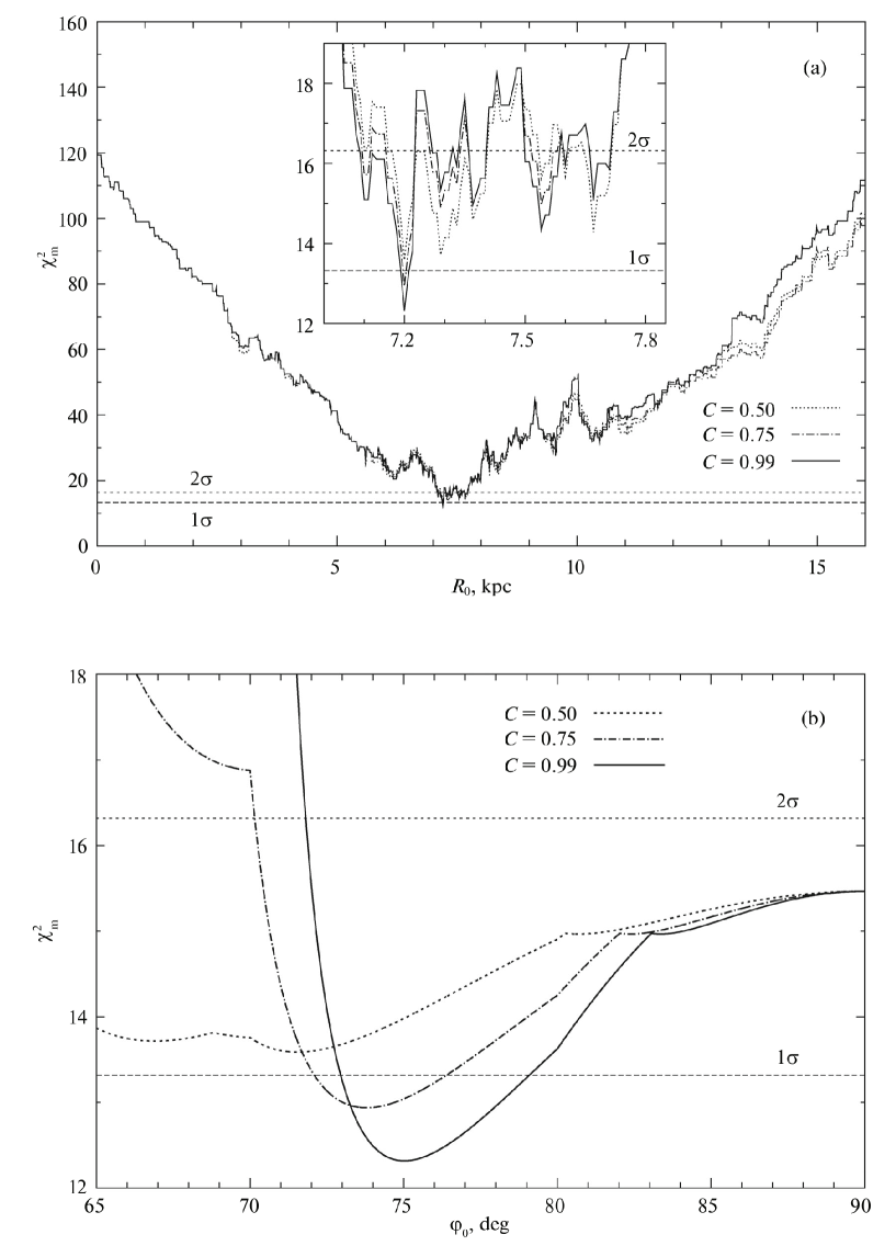
Fig. 9: Profiles of the objective function $\chi^{2}$ for the parameters $R_{0}$ (a) and $\varphi_{0}$ (b) at fixed values of the fraction of the component of the GC system with COA $C=0.50$, $0.75$, $0.99$ for the complete sample of clusters. The horizontal lines mark the $1\sigma$ and $2\sigma$ confidence levels for the solution at $C=0.99$.

Our attempts to solve the complete problem of optimizing the parameters of model (16) for different GC subsamples showed that $C\to 1$; the objective function acquires a distinct minimum (i.e., an unambiguous solution exists) only when the component with COA dominates ($C>0.5$) (Fig. 9). These results argue for the existence of COA in the GC system. Below we adopt $C=0.99$: as $C$ increases further, the estimates of the parameters barely change, but the confidence level at which the confidence region loses its connectivity slightly lowers.

Owing to the binning of the domain of definition of $\varphi$ for calculating the probabilities (18) and numbers $\nu_{i}$ and the presence of a sharp truncation at $|{\varphi}|={\varphi}_{0}$ in the component $f_{\text{c}}({\varphi})$ of model (16), the objective function $\chi^{2}(R_{0},\varphi_{0})$ turns out to be nonsmooth. For example, the $\chi^{2}_{\text{m}}(R_{0})$ profile (Fig. 9a) is, strictly speaking, a piecewise constant function, although the segments with a constant $\chi^{2}_{\text{m}}$ value near the global minimum are quite small (usually have a length $\Delta R_{0}\mathrel{\hbox{\hbox to0.0pt{\hbox{\lower 4.0pt\hbox{$\sim$}}\hss}\hbox{$<$}}}0.01$ kpc). In addition, the function $\chi^{2}_{\text{m}}(R_{0})$ experiences shallow but sharp oscillations. However, the solution of the problem is given by the narrow (the formal $1\sigma$ errors are $\sigma_{R_{0}}=0.01$–$0.04$ kpc) and fairly deep (unique up to the $1.4\sigma$ confidence level) minimum (Fig. 9a, Table 6).

The depth of the minimum in the $\chi^{2}_{\text{m}}(\varphi_{0})$ profile is limited by the difference between the value of this function at the right boundary of the domain of definition of $\chi^{2}_{\text{m}}(\pi/2)$, which does not depend on $C$, and the $\chi^{2}_{0}$ value as a function of $C$ (Fig. 9b). The significance of the minimum turns out to be only close to the marginal one: for example, for the complete GC sample it is $1.8\sigma$ (92.4%) at $C=0.99$ and grows weakly as $C$ increases further. The parameter $\varphi_{0}$ is limited from below much more strongly than from above (Fig. 9b). Note that when the COA is abandoned in the model or when the contribution of the component with COA is simply reduced greatly, the determination of the parameter $R_{0}$ becomes ambiguous (see the $\chi^{2}_{\text{m}}(R_{0})$ profile at $C=0.5$ in Fig. 9a).

The method was applied to the complete GC sample, to the northern ($b>0^{\circ}$) and southern ($b<0^{\circ}$) GCs separately, to the GCs with $[\text{Fe/H}]<-0.8$, and to the samples with combinations of these constraints. The constraint $[\text{Fe/H}]<-0.8$ stems from the fact that the higher-metallicity GCs form an oblate subsystem and can shift the results for a spherically symmetric model. The results obtained for these samples at $C=0.99$ are summarized in Table 6; the formal errors of the parameters for the $1\sigma$ level are given. Figure 10 presents the distributions of Galactocentric latitudes for the complete sample and the GC sample with $[\text{Fe/H}]<-0.8$ in comparison with the models (16) constructed for them and with the model without COA (15) at the optimal parameters $R_{0}$ and $\varphi_{0}$ (providing a minimum of the function $\chi^{2}$). Figure 10 illustrates good agreement of the observed $\varphi$ distributions with the model ones. Applying Pearson’s test leads to the same conclusion: for all of the samples considered at the optimal parameters $\chi_{0}^{2}<N_{\text{free}}$ , where $N_{\text{free}}=16$ for the GC samples without any constraints on $b$, $N_{\text{free}}=7$ for the samples of northern or southern GCs (see, e.g., Press et al. 1997).

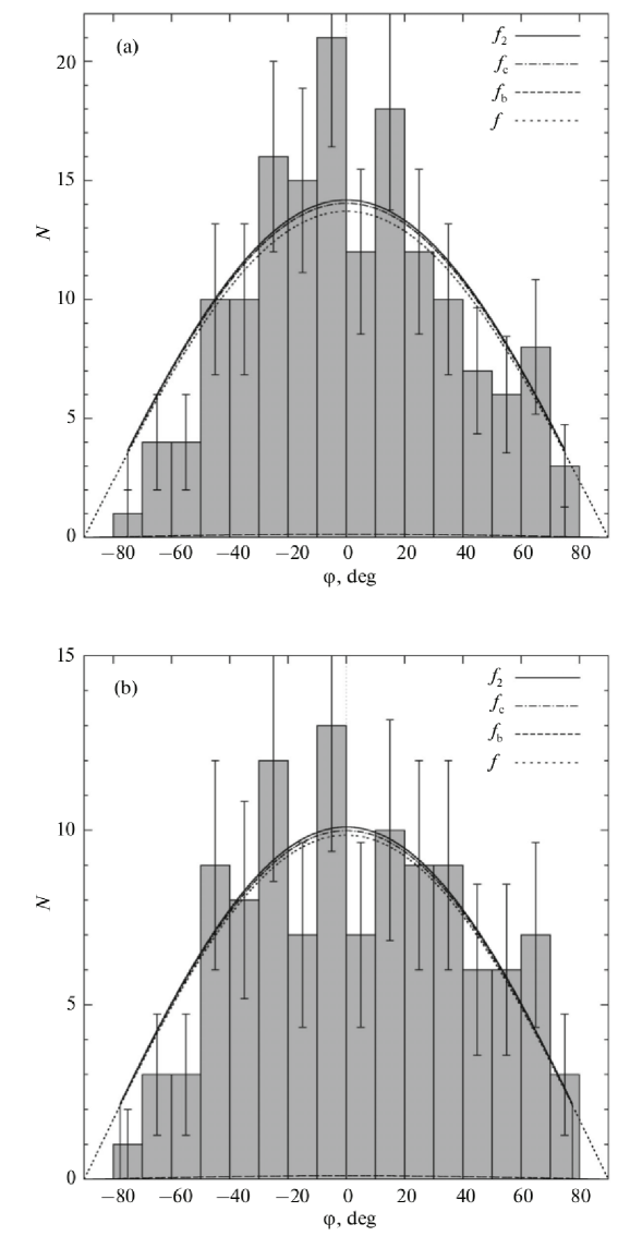
Fig. 10: Distribution of GCs in Galactocentric latitudes in comparison with the model $f_{2}(\varphi)$ that includes the component $f_{\text{c}}$ with COA and the component $f_{\text{b}}$ without COA and with the model $f(\varphi)$ in the absence of COA. $R_{0}$ and $\varphi_{0}$ are the values minimizing $\chi^{2}$ at $C=0.99$. (a) The complete sample ($N=157$), $R_{0}=7.20$ kpc, $\varphi_{0}=75\hbox{$.\!\!^{\circ}$}0$. (b) The sample with $[\text{Fe/H}]<-0.8$ ($N=113$), $R_{0}=7.22$ kpc, $\varphi_{0}=77\hbox{$.\!\!^{\circ}$}7$.

Apart from the formal estimates of $R_{0}{\color[rgb]{0,0,0}(\chi^{2}_{0})}$ corresponding to the global minimum of $\chi^{2}$, we also found the interval estimates of this parameter whose derivation we consider as a method of smoothing the oscillations of the function $\chi^{2}_{\text{m}}(R_{0})$. Here, we proceed from the following reasoning. The dependence $\chi^{2}_{\text{m}}(R_{0})$ has several local minima below the $\chi^{2}_{2}$ value ($2\sigma$ level). Random factors, for example, errors in the distances, can determine precisely which of them will be deepest. A characteristic feature of the function $\chi^{2}_{\text{m}}(R_{0})$ is its oscillation relative to the ${\approx}2\sigma$ level in the region of the global minimum in a comparatively narrow interval of $R_{0}$ outside which $\chi^{2}_{\text{m}}$ increases sharply (Fig. 9a). This gives grounds to rely on the confidence interval for the $2\sigma$ level when estimating $R_{0}$ . First we found the set of local minima of $\chi^{2}_{\text{m}}(R_{0})$ smaller than $\chi^{2}_{2}$ for which the values of $\varphi_{0}$ corresponding to them fell within the formal $1\sigma$ interval for $\varphi_{0}$ determined from the dependence $\chi^{2}_{\text{m}}(\varphi_{0})$. Then, we determined the intervals of $R_{0}$ in which the curves of these local minima did not exceed $\chi^{2}_{2}$ . The largest and smallest boundaries of these intervals were taken as the boundaries of the $2\sigma$ interval for estimating $R_{0}$ . We took the middle of the interval found in this way as the interval estimate of $R_{0}{\color[rgb]{0,0,0}(2\sigma)}$ and a quarter of its length as the $1\sigma$ error of this estimate. The interval estimates of $R_{0}$ are also given in Table 6.

Next, among the estimates of the parameters obtained we revealed obviously unreliable ones. These included the $R_{0}$ and $\varphi_{0}$ estimates based on the samples for which the function $\chi^{2}_{\text{m}}(\varphi_{0})$ did not reach the $1\sigma$ level at least on one side of the point estimate at $\varphi_{0}\geq 65^{\circ}$ (the subsamples of northern and southern low-metallicity GCs). [There were no such cases for the $\chi^{2}_{\text{m}}(R_{0})$ profiles.] The $\varphi_{0}$ estimates with a low significance of the minimum of $\chi^{2}_{\text{m}}(\varphi_{0})$ (with a confidence probability $P_{k}<85\%$) were also considered as unreliable ones. The values of $P_{k}$ corresponding to a $k\sigma$ level, $k=\sqrt{\chi^{2}_{k}-\chi^{2}_{0}}$ , were determined from the values of the function $\chi^{2}_{\text{m}}(\varphi_{0})=\chi^{2}_{k}$ at the boundaries of the interval ($\varphi_{0}=65^{\circ},90^{\circ}$) under consideration or at the points of its local maxima rightward and leftward of the point estimate. The values of $k$ and $P_{k}$ are given in Table 6, where “$+$” and “$-$” at $k$ denote the points of $\chi^{2}_{\text{m}}(\varphi_{0})$ rightward and leftward of the point estimate of $\varphi_{0}$ , respectively.

The remaining (more reliable) estimates of the parameters are highlighted in Table 6 in boldface. Based on them, we can draw the following conclusions with regard to the parameter $R_{0}$ . The formal and $2\sigma$-interval estimates are close ($|\Delta R_{0}|\leq 0.21$ kpc), without any clear shift of some relative to the others. The formal uncertainty in the estimates turned out to be low (within 0.2 kpc), but, as our numerical experiments showed, it was underestimated, especially for $R_{0}(\chi_{0}^{2})$. The $R_{0}$ estimates based on the northern and southern GCs and on the complete sample differ by no more than 0.2 kpc. Taking into account the more realistic errors of the interval estimates, this difference is insignificant. Besides, the sign of the north–south difference in the $R_{0}$ estimates is different for the formal and interval estimates. In any case, there is no evidence for $R_{0}$ estimated from the southern GCs being underestimated in comparison with those from the northern ones. Obviously, the inverse result formally obtained in Subsection 5.1 based on small samples of void-forming clusters is random in nature. The exclusion of metal-rich GCs barely changes the $R_{0}$ estimates.

The $R_{0}$ estimates highlighted in Table 6 were averaged with weights inversely proportional to the squares of the lengths of the confidence intervals. Since these estimates are not independent, as the error of the mean we took the square root of the weighted mean value of the squares of the errors in the estimates being averaged. By the error here we mean the positive or negative parts of the confidence interval for the $1\sigma$ level if they are different. We found the mean of four formal estimates, $\overline{R_{0}{\color[rgb]{0,0,0}(\chi^{2}_{0})}}=7.21\pm 0.01$ kpc, and the mean of the same number of interval estimates, $\overline{R_{0}{\color[rgb]{0,0,0}(2\sigma)}}=7.35\pm 0.10$ kpc. The difference in $\overline{R_{0}}$ for the two variants of estimates is insignificant.

This approach was tested by the Monte Carlo method. For each initial model we generated 1000 pseudo-random catalogs of GCs distributed spherically symmetrically with a radial density law ${\mathfrak{f}}(R_{\text{g}})\propto R_{\text{g}}^{-2.5}$ (Rastorguev et al. 1994) in the absence of COA ($\varphi_{0}=90^{\circ}$) and in its presence. The actual region of avoidance apparently goes beyond the COA, being nonaxisymmetric with a high probability (see Subsection 6.4), which manifests itself in a strong deficit of GCs seen within the COA in projection onto the $XZ$ plane compared to its projection onto the $YZ$ plane (Fig. 11). Therefore, we also considered a limiting case of this deficit as a model: the absence of GCs in the “trough of avoidance” $|\beta|>\beta_{0}$, where $\beta$ is the Galactocentric angular elevation of GCs above the Galactic plane in projection onto the $XZ$ plane. In the models we adopted $R_{0}=7.2$ kpc (the mean estimate in recent papers on GCs; see Table 8); $N$ and $\varphi_{0}$ were taken to correspond to the complete sample and the sample with $[\text{Fe/H}]<-0.8$ (Table 6). We took $\beta_{0}$ to be equal to $\varphi_{0}$ or $76^{\circ}$ (it corresponds to the largest value of the mentioned deficit; see Subsection 6.4). The results are presented in Table 7.

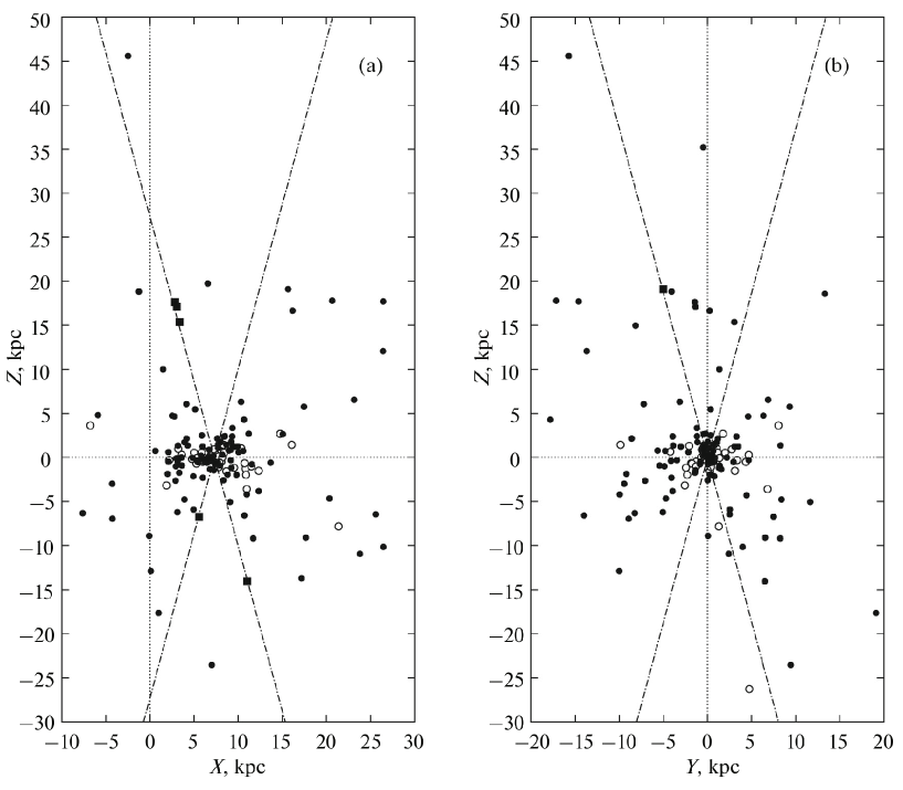
Fig. 11: Distribution of GCs and the contour (dash–dotted lines) of the COA ($\alpha_{0}=15\hbox{$.\!\!^{\circ}$}0$, $R_{0}=7.{\color[rgb]{0,0,0}3}$ kpc) in projection onto the $XZ$ (a) and $YZ$ (b) planes. The open circles are the clusters with $\text{[Fe/H]}>-0.8$; the filled symbols are the remaining clusters. The squares mark the clusters that are projected onto the COA cavity at $\alpha_{0}=15\hbox{$.\!\!^{\circ}$}0$ but are outside the COA at $\alpha_{0}={\color[rgb]{0,0,0}14\hbox{$.\!\!^{\circ}$}0}$. For each of the two projections there is one cluster that is projected onto the COA with $\alpha_{0}=15\hbox{$.\!\!^{\circ}$}0$ but is outside the figure.

Our numerical experiments showed both estimates of $R_{0}(\chi^{2}_{0})$ and $R_{0}{\color[rgb]{0,0,0}(2\sigma)}$ to be unbiased. The variance of the estimates strongly depends on the assumptions about the region of avoidance. The expectation that the presence of such a region made the $R_{0}$ estimates more effective was confirmed. The uncertainty in the $R_{0}{\color[rgb]{0,0,0}(2\sigma)}$ estimates in the presence of a region of avoidance is higher than the uncertainty in the $R_{0}(\chi^{2}_{0})$ estimates approximately by 30%. The formal errors in $R_{0}(\chi^{2}_{0})$ turned out to be clearly inadequate (underestimated approximately by an order of magnitude), obviously because the objective function is nonsmooth. The assumption that the formal errors in the interval estimates were more realistic was confirmed, but they were also underestimated.

Averaging the estimates based on real data $\overline{R_{0}(\chi^{2}_{0})}$ and $\overline{R_{0}(2\sigma)}$ with weights of $(1.3)^{2}$ and $1$, respectively, gives $\overline{R_{0}}=7.26$ kpc. Given that the actual region of avoidance is closer to the “trough” model (Section 6.4) and that $N=113$ corresponds to the sample with $[\text{Fe/H}]<-0.8$ more consistent with the assumption of spherical symmetry, based on our numerical experiments we take the uncertainty in this estimate to be $\pm 0.5$ kpc. Finally, we obtain an estimate of $\overline{R_{0}}=7.3\pm 0.5$ kpc by this method.

Table 7 shows that the parameter $\varphi_{0}$ in our numerical experiments is reconstructed within the limits of errors whose level is close to the formal ones (Table 6).

Although all of the approaches implemented in this paper lead to a positive difference of $\varphi_{0}$ from the northern and southern GCs, $\Delta\varphi_{0}\equiv\varphi_{0,\text{N}}-\varphi_{0,\text{S}}=+(6\hbox{${}^{\circ}$}$–$8\hbox{${}^{\circ}$})$ (Tables 1–6), this difference is found to be insignificant when the distribution of Galactocentric latitudes is modeled directly. The most reliable results (for the samples with $b>0^{\circ}$ and $b<0^{\circ}$) give $\Delta\varphi_{0}=+6\hbox{$.\!\!^{\circ}$}0\pm 4\hbox{$.\!\!^{\circ}$}2$ ($1.4\sigma$). (Note that for the northern GCs the significance of the minimum of $\chi^{2}_{\text{m}}(\varphi_{0})$ is low only in the sense of a constraint on $\varphi_{0}$ from above, but not from below.) Thus, we have no reason to believe that the northern and southern COA cavities differ significantly in angular size. In Fig. 10 we can see some deficit of southern GCs at $\varphi\mathrel{\hbox{\hbox to0.0pt{\hbox{\lower 4.0pt\hbox{$\sim$}}\hss}\hbox{$<$}}}-50\hbox{${}^{\circ}$}$. However, the Kolmogorov–Smirnov test shows that the distributions of southern and northern GCs in $\varphi$ differ insignificantly: the null hypothesis is rejected only at the 68 and 77% levels for the complete sample and the sample of metal-poor GCs, respectively.

The estimate of $\varphi_{0}=75\hbox{$.\!\!^{\circ}$}0^{+4\hbox{$.\!\!^{\circ}$}1}_{-2\hbox{$.\!\!^{\circ}$}1}$ based on all GCs was taken as the final one as having the greatest significance $P_{k}$ of the minimum of $\chi^{2}_{\text{m}}(\varphi_{0})$. Averaging the three estimates of $\varphi_{0}$ with the greatest $P_{k}$ (based on all GCs and on the samples with $b>0\hbox{${}^{\circ}$}$ and $b<0\hbox{${}^{\circ}$}$) using the same procedure as that for $R_{0}$ gives a smaller value, $\overline{\varphi_{0}}=73\hbox{$.\!\!^{\circ}$}6^{+4\hbox{$.\!\!^{\circ}$}1}_{-1\hbox{$.\!\!^{\circ}$}6}$, because the estimate based on the southern GCs ($\varphi_{0}={71\hbox{$.\!\!^{\circ}$}9}^{+3\hbox{$.\!\!^{\circ}$}7}_{-1\hbox{$.\!\!^{\circ}$}3}$) is formally more accurate. However, the latter is not revealing, because a random shift of the $\varphi_{0}$ estimate to smaller values must lead to a larger formal conditionality: from general considerations a wider COA is identified with greater confidence than a narrower one at the same GC sample size (see also Table 6).

6 DISCUSSION

The approaches considered in this paper (Subsections 4.2, 4.3, 5.1, 5.3) yield, on the whole, similar results. Let us discuss what conclusions they allow to draw and what further prospects for this method are.

6.1 The Existence of an Axial Zone of Avoidance

The existence of such a zone in the Galactic GC system is revealed when analyzing the distribution of locally maximal cylindrical voids (Section 4) and is confirmed by the results of modeling the distribution of Galactocentric latitudes (Subsection 5.3). Within the latter approach the $\chi^{2}$ minimization requires the dominance of the component with COA and the solution of the problem turns out to be unambiguous only under the condition of such dominance. The distinct minima of $\chi^{2}_{\text{m}}(\varphi_{0})$ for the most reliable solutions also confirm the existence of COA.

The probability that for a spherically symmetric GC distribution, i.e., for the distribution law (15), none of $N$ GCs falls into a double COA with a halfangle $\alpha_{0}$ is $P_{N}(0)=\cos^{N}\alpha_{0}$, because $2\int_{0}^{\pi/2-\alpha_{0}}\frac{\cos\varphi}{2}\,d\varphi=\cos\alpha_{0}$ . Then, $P_{157}(0)=0.43\%$ and $P_{118}(0)=1.7\%$ (the sample without GCs with $\text{[Fe/H]}>-0.8$ having an oblate distribution along the $Z$ axis). However, it is not sufficient to rely only on the statistics of the $\varphi$ distribution at some fixed $R_{0}$ in this question, because Pearson’s test applied to such a distribution does not reject the alternative model, the absence of COA, either: the probabilities to obtain the observed or larger deviations from such a model are 51 and 87% for the distributions on the upper and lower panels of Fig. 10, respectively, although the $\chi^{2}$ statistics in the absence of COA is nevertheless poorer (16.23 and 10.69, respectively) than that in its presence (12.32 and 8.66). At the same time, the value of $R_{0}$ obtained through general optimization is of crucial importance.

Using the results of our numerical experiments (Subsection 5.3), we can test the null hypothesis by determining, in the absence of a region of avoidance, the probability to obtain the same COA as that from real data or wider and, at the same time, a value of $R_{0}$ as close as that from real data or closer to the mean $\langle R_{0}\rangle_{\text{GC}}$ from papers based on an analysis of the spatial GC distribution (see Table 8). For $\langle R_{0}\rangle_{\text{GC}}=7.18$ kpc (from 1989–2014 papers) these probabilities at $N=113$ are 1.1 and 2.1% for $R_{0}(\chi^{2}_{0})$ and $R_{0}{\color[rgb]{0,0,0}(2\sigma)}$, respectively; for $\langle R_{0}\rangle_{\text{GC}}=7.32$ kpc (from 1975–2014 papers) they are 1.6 and 1.0%. At $N=157$ these probabilities are even lower: ${<}0.0$, 0.4, 0.5, and 0.1%, respectively. Thus, the hypothesis about the absence of a region of avoidance is rejected at least at the 98% level. Note that in the presence of a cone or trough of avoidance the hypotheses about obtaining similar results by chance are not rejected (the probabilities even for $N=113$ turn out to be in the intervals 5.4–16 and 18–41%, respectively).

Thus, a random realization of the zone of avoidance is unlikely. The fact that its axis will be orthogonal to the Galactic plane by chance is even less likely (Fig. 7).

Note that even the random nature of the zone of avoidance (which must not be ruled out completely) does not abolish the very fact of its existence at the present epoch, because the random errors in the distances to GCs at large $|b|$ are small (${\sim}0^{m}\!\!\!.\,1\approx 5\%$, see H10) compared to the sizes of the identified axial voids, nor does it abolish the fact that the position of the axis of this zone is close to the GC density maximum (Fig. 7, Tables 3, 4).

If the axial zone of avoidance is nevertheless caused dynamically, then how stable is it as a structure, given that some GCs can move in chaotic orbits (for example, NGC 6626; see Casetti-Dinescu et al. 2013)? In recent years the proper motions have been measured for many GCs, which has made it possible to calculate their orbits (see, e.g., Allen et al. 2006, 2008; Casetti-Dinescu et al. 2013). For example, in these three papers the meridional orbits are provided for a total of 25 GCs. This gives some statistics for answering the above question. During their orbital motion six of these GCs cross the region of a formal COA with $\alpha_{0}=15^{\circ}$. However, all these GCs are relatively close to the Galactic axis ($R_{\text{max}}=3$–8  kpc) and enter into the COA region at small distances from the Galactic plane: three GCs (NGC 6316, NGC 6528, and NGC 6626) at $|Z|\mathrel{\hbox{\hbox to0.0pt{\hbox{\lower 4.0pt\hbox{$\sim$}}\hss}\hbox{$<$}}}1$ kpc (Allen et al. 2006; Casetti-Dinescu et al. 2013), two GCs (NGC 4833 and NGC 6723) at $|Z|\mathrel{\hbox{\hbox to0.0pt{\hbox{\lower 4.0pt\hbox{$\sim$}}\hss}\hbox{$<$}}}2$ kpc (Allen et al. 2006, 2008), and only one GC (NGC 5968) at $|Z|\mathrel{\hbox{\hbox to0.0pt{\hbox{\lower 4.0pt\hbox{$\sim$}}\hss}\hbox{$<$}}}4$ kpc (Allen et al. 2008). Besides, these GCs spend an insignificant fraction of time in the COA, crossing it (often tangentially) near the pericenters of their orbits. In any case, the outer COA regions (at least at $|Z|\mathrel{\hbox{\hbox to0.0pt{\hbox{\lower 4.0pt\hbox{$\sim$}}\hss}\hbox{$>$}}}4$ kpc) seem stable structures from this viewpoint; only the inner parts of the COA ($1\mathrel{\hbox{\hbox to0.0pt{\hbox{\lower 4.0pt\hbox{$\sim$}}\hss}\hbox{$<$}}}|Z|\mathrel{\hbox{\hbox to0.0pt{\hbox{\lower 4.0pt\hbox{$\sim$}}\hss}\hbox{$<$}}}4$ kpc) can be periodically “washed out.” In the layer $|Z|\mathrel{\hbox{\hbox to0.0pt{\hbox{\lower 4.0pt\hbox{$\sim$}}\hss}\hbox{$<$}}}1$ kpc the COA is not revealed with confidence even at the present epoch, in agreement with the statistics of orbits that independently identifies this boundary. These results are largely explained by the fact that the stochastization of orbits is enhanced by the bar and the spiral structure, which predominantly affect, respectively, the GCs close to the Galactic center and the GCs with a low energy of their vertical oscillations (see the above papers). In contrast, the COA is revealed mainly by distant GCs at large $|Z|$. Note that stochastization does not always increase the probability of GC entry into the COA region: for example, the orbit of NGC 5968 in an axisymmetric potential crosses the COA by its loops more densely than in the case where the bar and spirals are taken into account (Allen et al. 2008). Obviously, this statistics of orbits, along with other arguments (see Subsection 5.2), stimulates the parametric modeling methods in which the location of clusters in the formal zone of avoidance is not ruled out completely, while the zone itself does not include the central region of the Galaxy.

6.2 The Quantity $R_{0}$

We determined $R_{0}$ by modeling the distribution of Galactocentric latitudes for GCs by two methods each of which has its advantages, difficulties, and weak points. The first method (least-squares optimization, Subsection 5.1) is based on a sample of clusters that in their $Z$ layers constrain best the position of the zone of avoidance. Other GCs, including those at small $|Z|$ where the axial structure of avoidance is not revealed unambiguously, are ignored. This makes the first method more refined in the sense of using the COA as a structural feature to determine $R_{0}$ (here, no information about the number density peak or the centroid of clusters is invoked). The absence of GCs close to the Galactic plane in the final sample offers yet another advantage: the problems of selection and extinction correction when determining the photometric distances are not significant here. However, this method requires a preselection of the set of those GCs that outline the axial structure using a special algorithm. At the same time, this method inherits the errors of the operation of the selection algorithm, in particular, the fall of objects with large deviations from the final axial direction into this set (Figs. 7, 8b) due to the discreteness of the GC system. In addition, the limited number of GCs in the Galaxy does not allow a denser partition into $Z$ layers to be performed and inevitably leads to a small size of the sample of GCs outlining the axial zone of avoidance. The latter, in turn, limits the statistical accuracy and robustness of the result (Table 5).

The second method of determining $R_{0}$ ($\chi^{2}$ minimization) uses not only the COA but also, indirectly, the fact of GC concentration toward the Galactic center (the observed distribution of latitudes $\varphi$ must be in best agreement with the model one at the system’s center even in the absence of COA). One advantage of the method is that it does not require any a priori data on the zone of avoidance except the general form of its model. Another advantage is the applicability of the method to a wide class of GC subsamples, including the complete GC sample, i.e., the possibility of using samples of a large size. This leads to statistically more accurate and robust $R_{0}$ estimates (Table 6) than those yielded by the first method. One of the shortcomings of $\chi^{2}$ minimization is that the objective function is nonsmooth, but this creates only computational difficulties. The use of GCs near the Galactic plane can be a more serious shortcoming in terms of systematic errors. Indeed, the observational incompleteness of GCs in the Galactic disk and especially the presence of a dust bar (Schultheis et al. 2014), which shields the GCs in the Galactic bar and behind it along the line of sight (Nikiforov and Smirnova 2013), can noticeably shift the apparent symmetry center of the GC system to the near side and, consequently, can underestimate $R_{0}$ . As has been mentioned in the Introduction, this is a potential source of systematic errors characteristic for the spatial methods of determining $R_{0}$ from GCs.

A truncation of the GC distribution behind the Galactic center, $X>R_{0}$, in contrast with the distribution at $X<R_{0}$ manifests itself for the layer $-0.58\leq Z<1.0$ kpc even in projection onto the $XZ$ plane (Fig. 7), with the truncation sharpness increasing with decreasing $|Z|$. Under a noticeable influence of such selection on the $\chi^{2}$-minimization result one might expect the $2\sigma$-interval estimates of $R_{0}$ to be smaller than the formal ones, because the former are not directly associated with the optimal position of the COA, while the latter are determined precisely by it. In reality, the reverse is true: the $2\sigma$-interval estimates, on average, turn out to be even slightly larger (by $0.14\pm 0.10$ kpc) than the formal estimates (Subsection 5.3). The exclusion of high-metallicity ($\text{Fe/H}]>-0.8$) GCs, for which the selection effect must be stronger, barely changes the $R_{0}$ estimates (Table 6). Finally, the first method of determining $R_{0}$ based on a sample of GCs among which there are no objects with $|Z|\leq 1.4$ kpc gives $R_{0}={7.29}^{+0.29}_{-0.28}$ kpc coincident with the result of the second method, $\overline{R_{0}}=7.3\pm 0.5$ kpc. All of this suggests that the observational incompleteness of GCs does not affect strongly the $\chi^{2}$-minimization results. Note that in both methods the minimum of the objective function establishing an optimal $R_{0}$ is identified unambiguously, in contrast to the method of maximizing the formal COA (cf. Fig. 1a with Figs. 8а and 9a).

As an estimate of $R_{0}$ from the COA in the distance scale (1) we take the result of the second method, ${R_{0}}=7.3\pm 0.5$ kpc, based on larger statistics and tested numerically. The distance scale (1) was calibrated in H10 (the catalog by Harris (1996), the 2010 version) using the data on GCs in M 31, i.e., under the assumption of some distance to this galaxy. This makes the calibration partly secondary. Let us rescale the results of Subsection 5.3 to

$$M_{V}(\text{HB})=0.165\,\text{[Fe/H]}+0.86,$$ (21)

with the primary calibration obtained in H10 from the most direct distance measurements within our Galaxy by comparing the scales (1) and (21) at the mean metallicity $[\text{Fe/H}]=-1.3$ for all GCs and at the mean metallicity $[\text{Fe/H}]=-1.5$ for GCs with $[\text{Fe/H}]<-0.8$. Then, $\overline{R_{0}(\chi^{2}_{0})}=7.17$ kpc and $\overline{R_{0}(2\sigma)}=7.31$. Averaging these estimates with weights of $(1.3)^{2}$ and $1$, we finally obtain

$${R_{0}}=7.2\pm 0.5\bigr{|}_{\text{stat}}\pm 0.3\bigr{|}_{\text{calib}}~{}\text{kpc}.$$ (22)

Here, the second (systematic) error reflects the $\pm 0^{m}\!\!\!.\,1$ uncertainty in the calibration of the distance scale (21) (see H10).

The estimate (22) is small in comparison with the present-day means $\langle R_{0}\rangle_{\text{best}}=(7.8$–$8.25)\pm(0.1$–$0.5)$ kpc (for references see Section 1), but not in comparison with other $R_{0}$ determinations based on the spatial distribution of GCs. Table 8 summarizes the estimates of this class published since 1975 and the averaged (see Nikiforov 2003, 2004) values, $\langle R_{0}\rangle_{\text{GC}}$ (GC stands for globular clusters), for some of their subsets (the systematic error of the methods was taken to be $\sigma_{\text{meth}}=0^{m}\!\!\!.\,2$). Our result agrees well with $\langle R_{0}\rangle_{\text{GC}}$ obtained from previous estimates. Table 8 shows that beginning from 1989 the $R_{0}$ estimates, being rescaled to (21), turn out to be close to one another and they all do not exceed 7.6 kpc. The mean of them $\langle R_{0}\rangle_{\text{GC}}=7.18\pm 0.24$ kpc is very close to our estimate (22). Averaging these estimates by taking into account (22), i.e., over the more homogeneous group of 1989–2016 results, leads to the current mean value of the spatial $R_{0}$ estimates from the data on GCs:

$$\langle R_{0}\rangle_{\text{GC}}=7.19\pm 0.2{\color[rgb]{0,0,0}2}\bigr{|}_{\text{\color[rgb]{0,0,0}stat, meth}}\pm 0.33\bigr{|}_{\text{\color[rgb]{0,0,0}calib}}~{}\text{kpc}.$$ (23)

Thus, our analysis of the spatial GC distribution leads to values of $R_{0}$ considerably smaller than the bulk of the results obtained by other methods. The causes of this discrepancy can be: (1) the underestimation of the present-day GC distance scale; (2) the neglect of the selection effect and/or other systematic errors in the analysis of the spatial GC distribution; and (3) the unrealistic assumption about a symmetry of the GC system and/or a shift of the central spatial features of this system relative to the Galactic “centers” determined in a different way. An attempt to explain the discrepancy only by the first cause leads to the assumption that the distance scale of GCs (and RR Lyrae variables “akin” to them in calibration) was underestimated by $(10$–$13)\pm 5\%$, i.e., by $(0^{m}\!\!\!.\,20$–$0^{m}\!\!\!.\,26)\pm 0^{m}\!\!\!.\,1$, which now seems not very plausible [see the calibration in H10 and a summary of distance scales in Francis and Anderson (2014)]. The second cause is more probable, but the closeness of the $R_{0}$ estimate fromthe COA in this paper to other recent spatial estimates from GCs argues against a strong influence of the selection effect on $R_{0}$ in this class of methods. Note that the disregarded systematics can also be in other methods, but it is unlikely to be able to strongly shift (increase) the “best” mean $\langle R_{0}\rangle_{\text{best}}$ due to the great variety of methods. In our view, the third (hypothetical) cause is not improbable. Although the inner part of the Galaxy seems a well-established system where the density peak of the visible matter may be deemed close to the barycenter (the center of mass), this assumption almost certainly breaks down on scales of tens of kpc due to its accretion and interaction with other galaxies of the Local group, which manifests itself, for example, as an outer disk warp (see, e.g., Bland-Hawthorn and Gerhard 2016). Therefore, the asymmetry of the GC system must not be ruled out completely, at least on this scale. The difference between $\langle R_{0}\rangle_{\text{best}}$ and $\langle R_{0}\rangle_{\text{GC}}$ may be due to a combination of all these causes. The question remains open.

Note that comparatively low values of $R_{0}$ have recently been obtained not only from an analysis of the spatial GC distribution but also by some other methods, for example, $R_{0}=7.52\pm 0.10\bigr{|}_{\text{\color[rgb]{0,0,0}stat}}\pm 0.35\bigr{|}_{\text{\color[rgb]{0,0,0}system}}$ kpc (Nishiyama et al. 2006) and $R_{0}=7.5\pm 0.3$ kpc (Francis and Anderson 2014) from red clump stars in the bulge, $R_{0}=7.25\pm 0.32$ kpc (Bobylev 2013) from the kinematics of star-forming regions near the solar circle, and $R_{0}=6.72\pm 0.39$ kpc (Branham 2014) from the kinematics of OB stars.

6.3 The Parameter $\varphi_{0}$

As the final result for this parameter we take the estimate of $\varphi_{0}=75\hbox{$.\!\!^{\circ}$}0^{+4\hbox{$.\!\!^{\circ}$}1}_{-2\hbox{$.\!\!^{\circ}$}1}$ derived in Subsection 5.3. Note that it is very close to $\varphi_{0}=75\hbox{$.\!\!^{\circ}$}3$ obtained by a different method, from the void-forming GCs of the axial zone of avoidance (the complete sample, see Subsection 5.1).

The error in the calibration of the GC distance scale does not distort the geometry of the zone of avoidance and, consequently, does not lead to any systematic error in the $\varphi_{0}$ estimate. Since the COA is identified by GCs at large $|Z|$, the selection effect for it is weak and can manifest itself only in a differential form: GCs in the far part of the COA surface with respect to the Sun can be revealed with a lower probability than those in the near part. In principle, this could lead to some overestimation of $\varphi_{0}$ and $R_{0}$ . However, the differential selection cannot be significant, because although the differential effect grows with $|b|$, the selection itself decreases sharply. Indeed, in the far (with respect to the COA) part of the Galaxy at $|Z|\mathrel{\hbox{\hbox to0.0pt{\hbox{\lower 4.0pt\hbox{$\sim$}}\hss}\hbox{$>$}}}1$ kpc many GCs have been detected at large distances (Figs. 5, 7).

6.4 The Shape of the Zone of Avoidance

The assumption about the existence of COA in the Galactic GC system arose from the fact that a deficit of clusters toward the region along the Galactic axis was noticed in projection onto the $XZ$ plane (Wright and Innanen 1972b). In Fig. 11a the GC distribution in this projection based on the H10 data is compared with the COA contour for the parameters $\alpha_{0}=15\hbox{$.\!\!^{\circ}$}0$ and $R_{0}=7.3$ kpc found in this paper. Indeed, the deficit of GCs in the axial biconical region is quite noticeable. However, this deficit does not manifest itself clearly in projection onto the $YZ$ plane also parallel to the COA axis (Fig. 11b). This is confirmed by the following statistics. The number of GCs within the COA (i.e., being projected onto the COA) is $N_{0}=13$ for the $XZ$ plane and $N_{0}=27$ for the $YZ$ plane. After the exclusion of clusters with $\text{[Fe/H]}>-0.8$, these numbers are 12 and 23, respectively, which gives a density contrast of 1.9. In this case, half of the GCs within the COA on the $XZ$ plane are very close to the formal COA contour and largely form the apparent COA outline. If we exclude such clusters, i.e., take $\alpha_{0}={\color[rgb]{0,0,0}14\hbox{$.\!\!^{\circ}$}0}$, then $N_{0}^{XZ}=6$ and $N_{0}^{YZ}=21$ (for the $XZ$ and $YZ$ planes, respectively); the contrast is then 3.5. How probable is it to obtain such numbers $N_{0}$ by chance?

The mean and variance of the number of clusters visible within an axisymmetric COA with a half-angle $\alpha_{0}$ for the distribution (14) are

$$\operatorname{\mathsf{M}}N_{0}=Nn_{0},\qquad\operatorname{\mathsf{D}}N_{0}=Nn_{0}(1-n_{0}),\qquad n_{0}=\frac{2\alpha_{0}}{\pi\cos\alpha_{0}}-\frac{1}{\cos\alpha_{0}}+1,$$

where $N$ is the total size of the GC sample (see Appendix A3). At $N=118$ (the sample without GCs with $\text{[Fe/H]}>-0.8$) and $\alpha_{0}=14\hbox{$.\!\!^{\circ}$}0$ we obtain $\operatorname{\mathsf{M}}N_{0}=15.3\pm 3.{\color[rgb]{0,0,0}7}$. The excess of $N_{0}^{YZ}=21$ above $\operatorname{\mathsf{M}}N_{0}$ can be explained by chance: the probability $P(N_{0}\geq 21)={\color[rgb]{0,0,0}8.1\%}$ (in accordance with the binomial distribution) is not low. However, the underestimation of $N_{0}^{XZ}=6$ with respect to $\operatorname{\mathsf{M}}N_{0}$ is more significant: $P(N_{0}\leq 6)=4.1\times 10^{-3}$, i.e., the hypothesis about an axisymmetric COA when projected onto the $XZ$ plane is rejected with a probability of 99.59%. The probability for such a COA to obtain the same or larger difference for the two projections by chance approximately is $P(N_{0}^{XZ}\leq 6)\cdot P(N_{0}^{YZ}\geq 21)=3.{\color[rgb]{0,0,0}3}\times 10^{-4}$.

These results suggest that the axial zone of avoidance in the Galactic GC system is not strictly axisymmetric but is elongated in a direction approximately orthogonal to the $X$ axis, i.e., the Galactic center–anticenter line. We apparently owe the very fact of the detection of a zone of avoidance precisely to this combination of circumstances. First, if the latter at the present epoch were not oriented (by chance) parallel to one of the planes of the universally accepted Galactic cartesian coordinate system, then it would probably be noticed much later (Fig. 11b illustrates how difficult it is to suspect its presence for an “unfortunate” projection). Second, if the zone of avoidance were exactly axisymmetric (conical), then the observed surface density contrast $\widetilde{C}_{0}$ of GCs visible within the COA with respect to the remaining part of the GC system would be too weak and would not differ significantly from unity even in projection onto a plane parallel to the COA axis: $\operatorname{\mathsf{M}}\widetilde{C}_{0}=0.80$, $\sigma(\widetilde{C}_{0})=0.21$ and $\operatorname{\mathsf{M}}\widetilde{C}_{0}=0.82$, $\sigma(\widetilde{C}_{0})=0.22$ for $\alpha_{0}=15\hbox{$.\!\!^{\circ}$}0$ and $14\hbox{$.\!\!^{\circ}$}0$, respectively; the means and standard errors of the $\widetilde{C}_{0}$ estimate at $N=118$ are specified here [see Appendix A3, Eqs. (48) and (47)]. In contrast, when projected onto a plane inclined to the COA axis, the density contrast will be even weaker, because the central (denser) region of the GC system will occupy a larger fraction of the COA area. Thus, the COA would not be noticeable in projection onto any plane and could be detected only in a three-dimensional analysis. In reality, owing to the elongation of the zone of avoidance, the observed contrast for the $XZ$ plane is much stronger and differs significantly from unity: $\widetilde{C}_{0}=0.57\pm 0.17$ at $\alpha_{0}=15\hbox{$.\!\!^{\circ}$}0$ and $\widetilde{C}_{0}=0.29\pm 0.12$ at $\alpha_{0}={\color[rgb]{0,0,0}14\hbox{$.\!\!^{\circ}$}0}$; therefore, it was noticed [here, we use Eqs. (44) and (46) from Appendix A3]. Note that the latter value of $\widetilde{C}_{0}$ also differs significantly from $\operatorname{\mathsf{M}}\widetilde{C}_{0}=0.82$. For the $YZ$ plane the contrast is even reverse, $\widetilde{C}_{0}=1.21\pm 0.29$ and $1.18\pm 0.28$ at $\alpha_{0}=15\hbox{$.\!\!^{\circ}$}0$ and ${\color[rgb]{0,0,0}14\hbox{$.\!\!^{\circ}$}0}$, respectively, but it differs insignificantly from unity.

The subject matter being discussed is closely related to the question about the detectability of similar regions of avoidance in the GC systems of other galaxies, because only an analysis of the cluster distribution in the plane of the sky is accessible in this case. We will assume that the region of avoidance is revealed at a statistically significant level if

$$\frac{\sigma(\widetilde{C}_{0})}{1-\widetilde{C}_{0}}<\frac{1}{3}.$$ (24)

Suppose that a galaxy is observed from an optimal angle, i.e., edge-on. In the case of an axisymmetric double COA, substituting Eq. (47) and, to simplify the estimation, Eq. (43) for the asymptotic value $C_{0}$ of the observed contrast $\widetilde{C}_{0}$ into (24), we then obtain a constraint on the number of GCs:

$$N>N_{3\sigma}=\frac{9\cos^{2}\alpha_{0}}{(1-\cos\alpha_{0})^{2}}\cdot\frac{2\alpha_{0}+\pi\cos\alpha_{0}-\pi}{\pi-2\alpha_{0}}.$$ (25)

The minimum number of GCs is $N_{3\sigma}=1.15\times 10^{3}$ at $\alpha_{0}=15\hbox{$.\!\!^{\circ}$}0$ ($C_{0}=0.7956$) and $N_{3\sigma}=1.4{\color[rgb]{0,0,0}3}\times 10^{3}$ at $\alpha_{0}={14\hbox{$.\!\!^{\circ}$}0}$ ($C_{0}=0.8090$). Thus, provided that the axis of the COA lies in the plane of the sky, it can be reliably detected only in rich GC systems that are rare among spiral galaxies; in any case, the parent galaxy must be massive, with an absolute magnitude $M_{V}\mathrel{\hbox{\hbox to0.0pt{\hbox{\lower 4.0pt\hbox{$\sim$}}\hss}\hbox{$<$}}}-21{{}^{m}\!\!\!.\,}3$ (see, e.g., Figs. 5.5 and 5.6 in the book by Ashman and Zepf (2008)).

If the zone of avoidance is nonaxisymmetric (elongated), then a large $N$ is not required for its detection. Substituting Eqs. (43) and (46) into (24), we derive the constraint

$$N>N_{3\sigma}=\frac{9n_{0}}{1-n_{0}}\left(\frac{\pi-2\alpha_{0}}{2\alpha_{0}-\pi n_{0}}\right)^{2}.$$ (26)

Taking the observed contrasts to be $C_{0}=0.57$ ($n_{0}=0.102$, $\alpha_{0}=15\hbox{$.\!\!^{\circ}$}0$) and $C_{0}=0.29$ ($n_{0}=0.0508$, $\alpha_{0}={\color[rgb]{0,0,0}14\hbox{$.\!\!^{\circ}$}0}$), we find $N_{3\sigma}=168$ and $3{\color[rgb]{0,0,0}1}$, respectively. Thus, such zones of avoidance can also be detected in principle in moderately populated GC systems, but this additionally requires that the line of sight lie almost in the plane along which the zone is elongated, which sharply reduces the detection probability. The latter also depends on the factors causing the elongation.

The nonaxisymmetric structure of the zone of avoidance in the Galactic GC system may be due to the influence of the Magellanic Clouds (MCs). This assumption is consistent with some recent results. For example, there is evidence for the association of some of the halo GCs with the Magellanic plane or the Vast Polar Structure (see, e.g., Pawlowski et al. 2014). Yankelevich (2014) showed that Galactic GCs could even change the direction of their rotation to the opposite (retrograde) one under the gravitational perturbation from the MCs. Our assumption is also supported by the fact that in projection onto the $XZ$ plane the LMC is within the zone of avoidance, while the SMC is close to its contour (Figs. 6, 7). The passage of the MCs through the southern part of the Galactic halo at the present epoch may also explain the less regular shape of the southern cavity of the zone of avoidance (cf. the same figures).

The possibility that the central trough in the GC distribution orthogonal to the $X$ axis that was identified by Francis and Anderson (2014, below referred to as FA14) is a manifestation of the elongated zone of avoidance must not be ruled out. However, the status of this FA14 result is not quite clear. The trough was identified not during the spatial analysis but as one of the dips in the GC distribution in $X$ coordinate subjected to Gaussian smoothing. This dip appears distinct and “central” only when using the author’s catalog of GC distances but not for the catalogs of H10 and Bica et al. (2006): for H10 the dip is shallow and double, at $X_{0}\approx-0.2$ and $-1.0$ kpc ($X_{0}\equiv X-7.4\text{~{}kpc}$); for the catalog by Bica et al. (2006) the dip is more pronounced but lies at $X_{0}\approx-0.7$ kpc and then $R_{0}=6.7$ kpc (cf. Figs. 3 and 4 in FA14). The distance scale adopted in FA14 differs from the distance scales of the two other catalogs in that, being quadratic in metallicity, it assigns smaller distances to metal-rich GCs (see Fig. 1 in FA14), which are located predominantly in the central Galactic region. This displaces such GCs closer to the Sun, which in combination with the nondetectability of GCs in the far part of the bar and behind the bar (Nikiforov and Smirnova 2013) can lead to the “trough effect.” The extent to which the trough is attributable precisely to the GCs close to the center is not pointed out directly in FA14 (the constraints on the Galactocentric distance was imposed only from above, with the strongest one being 10 kpc), but our assumption is supported by the fact that the central dip for the sample of metal-poor GCs from the FA14 catalog is indistinct and almost merges with the neighboring dip at $X_{0}\approx-0.8$ kpc (Fig. 3 in FA14). The zone of avoidance considered in this paper is revealed, on the contrary, by GCs outside the Galactic bulge ($|Z|>1$ kpc). Unfortunately, the question about the statistical significance of the central dip as a structural feature for the constructed GC distribution in $X$ is not considered in FA14.

6.5 Prospects for the Method

In future, it would be desirable to use some modeling procedures that do not require any obligatory constraints on the GC sample. The $\chi^{2}$ minimization belongs to these procedures, but the objective function for it turns out to be nonsmooth. This shortcoming can be overcome by passing to the maximum likelihood method (MLM). Attempts to apply it for model (16) (Nikiforov and Agladze 2013) confirm the existence of a region of avoidance: $\varphi_{0}=77\hbox{$.\!\!^{\circ}$}4^{+2\hbox{$.\!\!^{\circ}$}5}_{-1\hbox{$.\!\!^{\circ}$}7}$ for the complete GC sample and $\varphi_{0}=76\hbox{$.\!\!^{\circ}$}8^{+3\hbox{$.\!\!^{\circ}$}3}_{-1\hbox{$.\!\!^{\circ}$}0}$ for the sample with $[\text{Fe/H}]<-0.8$. In this case, however, the $R_{0}$ estimates turned out to be generally shifted (6.01–7.02 kpc) due to the presence of a high hump in the profile of the logarithmic likelihood function ${\cal L}_{\text{m}}(R_{0})\equiv-\ln L_{\text{m}}(R_{0})$ at slightly larger $R_{0}$ (i.e., in the region of the highest GC density). The ${\cal L}_{\text{m}}(R_{0})$ profile leftward of the point estimate does not reach even the $2\sigma$ level (in contrast to the  $\chi^{2}_{\text{m}}(R_{0})$ profile). Studies have shown that the high sensitivity of the likelihood function to the location of central GCs (with small $|Z|$) at $|\varphi|$ very close to $90^{\circ}$ is responsible for the first effect. In this case, at the corresponding $R_{0}$ the probabilities to find such clusters according to model (16) are low at any values of other parameters. This gives the spikes in ${\cal L}_{\text{m}}(R_{0})$. When using the $\chi^{2}$ minimization, nothing of the kind occurs due to the smoothing: at $\varphi_{0}$ slightly larger than $80^{\circ}$ the terms $\frac{({\nu}_{i}-N{p}_{i})^{2}}{N{p}_{i}}$ for such GCs are not too large. The second effect is caused by the systematic drop in ${\cal L}_{\text{m}}(R_{0})$ as $R_{0}$ recedes from the true value due to the appearance of an increasingly large number of GCs at small $|\varphi|$, for which the occurrence probability according to (16) is maximal. The $\chi^{2}$ statistics tests the shape of the observed $|\varphi|$ distribution, which is strongly deformed as $R_{0}$ recedes from the true one and poorly corresponds to model (16) at any values of other parameters; therefore, $\chi^{2}_{\text{m}}(R_{0})$ does not fall off to the edges of the $R_{0}$ interval considered (Fig. 9a). Thus, the $\chi^{2}$ minimization turned out to be a more efficient estimator for model (16). For these reasons, we do not use the results obtained by the MLM in this paper.

However, the introduction of a more adequate model for the bulge component of the GC system can make the MLM efficient. This was highly desirable for the solution of our problem in a more general form.

The sharp truncations of distribution (16) at $\varphi=|\varphi_{0}|$ lead to the nonsmoothness of any objective function. The introduction of blurred truncation boundaries, which may also turn out to be more physical, would allow the problem to be solved.

Using a smooth objective function will allow more difficult problems (under more general assumptions), including the modeling of the zone of avoidance when abandoning the assumption of an axial symmetry, to be solved. Note that allowance for the elongation of the zone of avoidance will not shift the region of intersection of the zone projection onto the $XY$ plane with the $X$ axis, i.e., will not affect significantly the $R_{0}$ estimate.

7 CONCLUSIONS

The possibility of the presence of a double cone of avoidance (COA) in the globular cluster (GC) system of the Galaxy oriented along the Galactic rotation axis was considered previously in the literature. This direction was not developed further, but the only use of this structural feature to determine the distance to the Galactic center ($R_{0}$) in Sasaki and Ishizawa (1978) continued to be taken into account in the context of the $R_{0}$ problem. The main goal of this paper is to check whether an axial zone of avoidance exists in the GC system and to perform its parametrization that includes the new determination of $R_{0}$ as its parameter from currently available data (the catalog by Harris (1996), the 2010 version).

We showed that applying the method of maximizing the formal COA in Sasaki and Ishizawa (1978) generally led to an incorrect result because of the off-axis COAs due to the discreteness of the GC system. The presence of several approximately equal formal COAs revealed by the maximization method does not allow the existence of an axial zone of avoidance to be judged with confidence.

To check whether this zone was real, we represented the voids in the GC system by a set of largest-radius meridional cylindrical voids. As a result of our separate and joint analyses of the northern and southern voids, we managed to identify an ordered axial zone of avoidance and constructed the maps of its section by a meridional plane. The results obtained argue for the existence of a zone of avoidance for GCs along the Galactic axis (outside the small central region) that is close in shape to a double cone. The northern and southern COA cavities manifest themselves independently and with similar parame- ters. The position of the COA vertex is close to the position of the GC number density maximum.

Modeling the distribution of Galactocentric latitudes for GCs allows the optimal position of the axial COA to be unambiguously identified and leads to the following estimates of the parameters: $\varphi_{0}=75\hbox{$.\!\!^{\circ}$}0^{+4\hbox{$.\!\!^{\circ}$}1}_{-2\hbox{$.\!\!^{\circ}$}1}$, i.e., the COA half-angle $\alpha_{0}={15\hbox{$.\!\!^{\circ}$}0}^{+2\hbox{$.\!\!^{\circ}$}1}_{-4\hbox{$.\!\!^{\circ}$}1}$, ${R_{0}}=7.3\pm 0.5$ kpc. The southern COA cavity can be wider ($\alpha_{0}\approx 18\hbox{${}^{\circ}$}$) than the northern one ($\alpha_{0}\approx 12\hbox{${}^{\circ}$}$), but this difference is not significant. Comparison of the modeling results for various techniques and GC samples shows that the observational incompleteness of GCs affects insignificantly the $R_{0}$ estimate. A correction to the H10 calibration of the GC distance scale based on Galactic objects leads to an estimate of ${R_{0}}=7.2\pm 0.5\bigr{|}_{\text{stat}}\pm 0.3\bigr{|}_{\text{calib}}~{}\text{kpc}$. The latter is, on average, smaller than the present-day $R_{0}$ estimates but agrees well with $R_{0}$ deduced by analyzing the spatial GC distribution ($\langle R_{0}\rangle_{\text{GC}}=7.19\pm 0.22\bigr{|}_{\text{stat, meth}}\pm 0.33\bigr{|}_{\text{calib}}$ kpc).

As the maps of the zone of avoidance suggest, its southern cavity has a less regular shape than the northern one, which may be due to the influence of the Magellanic Clouds. Comparison of the GC distributions on two meridional planes revealed evidence for the elongation of the zone of avoidance in a direction orthogonal to the center–anticenter direction. This nonaxisymmetric structure may be caused by the same factor.

Our numerical experiments showed that in the absence of a region of avoidance the probability to obtain the same COA as that from real data or wider and, at the same time, $R_{0}$ estimates as close as those from real data or closer to the mean $\langle R_{0}\rangle_{\text{GC}}$ does not exceed 2%.

In external galaxies even when they are seen edge-on an axisymmetric COA can be detected only for rich GC systems ($N_{\text{GC}}>10^{3}$). Nonaxisymmetric zones of avoidance can also be revealed in principle in moderately populated GC systems, but only at a (lucky) orientation of the elongation of the zone along the line of sight.

APPENDIX

A1. Distribution of the Absolute Value of the Galactocentric Latitude

Obviously, the probability density of the random variable $\Phi$, the absolute values of the Galactocentric latitude $\varphi$, for a spherically symmetric GC distribution without any COA differs from the law (15) only by the normalization:

$$f\left({|\varphi|}\right)=\cos{\varphi}.$$ (27)

The mean of $\Phi$ is then

$$\operatorname{\mathsf{M}}\Phi=\int\limits^{\pi/2}_{0}{\varphi\cos{\varphi}\,d\varphi}=\frac{\pi}{2}-1\approx 0.5708\approx 32\hbox{$.\!\!^{\circ}$}70.$$ (28)

A2. Distribution of the Largest of the Two Absolute Values
of the Galactocentric Latitudes

Consider the random variable $\Phi_{\text{m}}=\max(\Phi_{1},\Phi_{2})$, where $\Phi_{1}$ and $\Phi_{2}$ are the arguments of the pair of members (the absolute values of the latitudes for the pair of globular clusters) extracted at random from a population with the argument $\Phi$ obeying the law (27). Let us find the probability density $f(\varphi_{\text{m}})$ of the random variable $\Phi_{\text{m}}$ . (The quantities $\varphi_{\text{m}}$ defined for the axial voids in Subsections 4.2 and 4.3 may be considered as the values of the random variable $\Phi_{\text{m}}$ in the absence of COA.)

Since the order in the pair of members is unimportant, we will assign the indices in each pair of $\phi_{1}$ and $\phi_{2}$ values of the random variables $\Phi_{1}$ and $\Phi_{2}$, for example, according to the rule $\phi_{1}\geq\phi_{2}$ . Then, $\varphi_{\text{m}}=\phi_{1}$ . In view of (27), the probability that $\Phi_{\text{m}}$ will fall into the interval $[\varphi_{\text{m}},\varphi_{\text{m}}+d\varphi_{\text{m}}]$ is defined as

$$\begin{split}P(\varphi_{\text{m}}\leq\Phi_{\text{m}}<\varphi_{\text{m}}+d\varphi_{\text{m}})&=P(\phi_{1}\leq\Phi_{\text{m}}<\phi_{1}+d\phi_{1})=\\ &=P(\phi_{1}\leq\Phi_{1}<\phi_{1}+d\phi_{1})\cdot P(\Phi_{2}\leq\phi_{1})=\\ &=c^{\prime}_{1}\cos\phi_{1}\int\limits^{\phi_{1}}_{0}\cos\phi\,d\phi=c_{1}\sin 2\phi_{1}=c_{1}\sin 2\varphi_{\text{m}}\,,\end{split}$$ (29)

where $c^{\prime}_{1}$ and $c_{1}$ are the variants of the normalization constants. The choice of a different rule ($\phi_{2}\geq\phi_{1}$) and the permutation of indices 1 and 2 in (29) do not change the result. Given the normalization

$$1=c_{1}\int\limits^{\pi/2}_{0}{\sin 2\varphi_{\text{m}}\,d\varphi_{\text{m}}}=c_{1}\,,$$

we finally obtain

$$f(\varphi_{\text{m}})=\sin{2\varphi_{\text{m}}}\,.$$ (30)

Then, the mean of $\Phi_{\text{m}}$ is

$$\operatorname{\mathsf{M}}\Phi_{\text{m}}=\int\limits^{\pi/2}_{0}{\varphi_{\text{m}}\sin{2\varphi_{\text{m}}}\,d\varphi_{\text{m}}}=\frac{\pi}{4}\,,$$ (31)

the variance of $\Phi_{\text{m}}$ is

$$\operatorname{\mathsf{D}}\Phi_{\text{m}}=\int\limits^{\pi/2}_{0}{\left(\varphi_{\text{m}}-\frac{\pi}{4}\right)^{2}\sin{2\varphi_{\text{m}}}\,d\varphi_{\text{m}}}=\frac{\pi^{2}-8}{16},$$ (32)

and the standard deviation is

$$(\operatorname{\mathsf{D}}\Phi_{\text{m}})^{1/2}=\frac{\sqrt{\pi^{2}-8}}{4}\approx 0.3418\approx 19\hbox{$.\!\!^{\circ}$}59.$$ (33)

A3. Surface Density Contrast between Globular Clusters Inside and Outside the Cone of Avoidance when Observed in Projection onto a Plane Parallel to the Cone Axis

In a spherically symmetric GC system with a double axial COA, i.e., with the distribution of Galactocentric latitudes (14), the number of GCs seen in projection onto the COA, $N_{0}$, does not depend on the radial density law ${\mathfrak{f}}(R_{\text{g}})$ if the plane of projection is parallel to the COA axis. Indeed, in this case, the radius drawn from the system’s center cannot cross the boundary of the region of space being projected onto the COA, because two planes passing through the center form this boundary; the radius can only lie at the boundary. $N_{0}$ is then completely determined by the total number of GCs in the system, $N$, and the fraction, $n_{0}$, of the system’s volume being projected onto the COA, $V_{0}$ :

$$N_{0}=Nn_{0}\,,\qquad n_{0}=\frac{V_{0}}{V},$$ (34)

where $V$ is the volume of the sphere minus the double cone. If the opening angle of the latter is $\alpha_{0}$ , then

$$V=\frac{4}{3}\pi a^{3}\cos\alpha_{0}\,,$$ (35)

where $a$ is the radius of the GC system.

The volume $V_{0}$ is the difference between the volume of the double azimuthal sector of the sphere

$$V_{\text{as}}=\frac{4}{3}\pi a^{3}\cdot\frac{4\alpha_{0}}{2\pi}=\frac{8}{3}a^{3}\alpha_{0}$$ (36)

and the volume of the double spherical sector

$$V_{\text{ss}}=2\int^{a}_{0}\!\int^{2\pi}_{0}\!\!\!\int^{\pi/2}_{\varphi_{0}}R^{2}_{\text{g}}\cos\varphi\,dR_{\text{g}}\,d\theta\,d\varphi=\frac{4}{3}\pi a^{3}(1-\cos\alpha_{0}),$$ (37)

where $\varphi_{0}=\pi/2-\alpha_{0}$ . Then,

$$V_{0}=\frac{4}{3}a^{3}(2\alpha_{0}+\pi\cos\alpha_{0}-\pi),$$ (38)

$$n_{0}=\frac{2\alpha_{0}}{\pi\cos\alpha_{0}}-\frac{1}{\cos\alpha_{0}}+1.$$ (39)

Hence the fraction of the system’s volume that is not projected onto the COA is

$$n_{1}=1-n_{0}=\frac{1}{\cos\alpha_{0}}-\frac{2\alpha_{0}}{\pi\cos\alpha_{0}}.$$ (40)

Given $n_{0}$ and $n_{1}$, it is easy to find the GC surface density inside the COA

$$\mu_{0}=\frac{N_{0}}{S_{0}}=\frac{Nn_{0}}{\pi a^{2}}\cdot\frac{2\pi}{4\alpha_{0}}=\frac{Nn_{0}}{2\alpha_{0}a^{2}}$$ (41)

and the surface density outside the COA

$$\mu_{1}=\frac{Nn_{1}}{S_{1}}=\frac{Nn_{1}}{\pi a^{2}}\frac{2\pi}{2\pi-4\alpha_{0}}=\frac{Nn_{1}}{a^{2}(\pi-2\alpha_{0})},$$ (42)

where $S_{0}$ and $S_{1}$ are the areas of the projection of the double spherical sector and the projection of the part of the GC system outside the COA, respectively. Hence, given (39) and (40), we obtain a theoretical value of the surface density contrast inside the COA with respect to the remaining part of the GC system:

$$C_{0}=\frac{\mu_{0}}{\mu_{1}}=\frac{n_{0}}{n_{1}}\frac{\pi-2\alpha_{0}}{2\alpha_{0}}=1-\frac{\pi}{2\alpha_{0}}\,(1-\cos\alpha_{0}).$$ (43)

Counting the GCs that fell within the COA gives an estimate of the contrast from observations:

$$\widetilde{C}_{0}=\frac{N_{0}}{N-N_{0}}\frac{\pi-2\alpha_{0}}{2\alpha_{0}}.$$ (44)

Since $N_{0}$ as a random variable obeys a binomial distribution,

$$\operatorname{\mathsf{M}}N_{0}=Nn_{0},\qquad\operatorname{\mathsf{D}}N_{0}=Nn_{0}(1-n_{0}).$$ (45)

Using (45), it is easy to find the statistical error of the $\widetilde{C}_{0}$ estimate from the error propagation formula

$$\sigma(\widetilde{C}_{0})=\frac{\sqrt{n_{0}}\,(\pi/2\alpha_{0}-1)}{\sqrt{N}(1-n_{0})^{3/2}}.$$ (46)

In general, we may adopt $n_{0}=N_{0}/N$ to estimate the uncertainty in the observed contrast. In the case of COA, substituting Eq. (39) for $n_{0}$, we obtain

$$\sigma(\widetilde{C}_{0})=\frac{\pi\cos\alpha_{0}}{2\alpha_{0}\sqrt{N}}\sqrt{\frac{2\alpha_{0}+\pi\cos\alpha_{0}-\pi}{\pi-2\alpha_{0}}}.$$ (47)

For the same case, given (43)–(45), we find the mean of the observed contrast:

$$\operatorname{\mathsf{M}}\widetilde{C}_{0}(N_{0})\approx\widetilde{C}_{0}(\operatorname{\mathsf{M}}N_{0})+\frac{1}{2}\widetilde{C}^{\prime\prime}_{0}(\operatorname{\mathsf{M}}N_{0})\operatorname{\mathsf{D}}N_{0}=C_{0}\left[1+\frac{1}{N(1-n_{0})}\right],$$ (48)

i.e., $C_{0}=\lim\limits_{N\to\infty}\operatorname{\mathsf{M}}\widetilde{C}_{0}$ .

REFERENCES

1. T. A. Agekyan, Probability Theory for Astronomers and Physicists (Nauka, Moscow, 1974) [in Russian].

2. C. Allen, E. Moreno, and B. Pichardo, Astrophys. J. 652, 1150 (2006).

3. C. Allen, E. Moreno, and B. Pichardo, Astrophys. J. 674, 237 (2008).

4. K. M. Ashman and S. E. Zepf, Globular Cluster Systems (Cambridge Univ. Press, Cambridge, UK, 2008).

5. B. S. Avedisova, Astron. Rep. 49, 435 (2005).

6. E. Bica, C. Bonatto, B. Barbuy, and S. Ortolani, Astron. Astrophys. 450, 105 (2006).

7. J. Bland-Hawthorn and O. Gerhard, Ann. Rev. Astron. Astrophys. 54, 529 (2016).

8. V. V. Bobylev, Astron. Lett. 39, 95 (2013).

9. T. V. Borkova and V. A. Marsakov, Astron. Rep. 44, 665 (2000).

10. R. L. Branham, Jr., Astrophys. Space. Sci. 353, 179 (2014).

11. D. I. Casetti-Dinescu, T. M. Girard, L. Jílková, W. F. van Altena, F. Podestá , and C. E. López, Astron. J. 146, 33 (2013).

12. T. Foster and B. Cooper, ASP Conf. Ser. 438, 16 (2010).

13. C. Francis and E. Anderson, Mon. Not. R. Astron. Soc. 441, 1105 (2014).

14. C. S. Frenk and S. D. M. White, Mon. Not. R. Astron. Soc. 198, 173 (1982).

15. R. Genzel, F. Eisenhauer, and S. Gillessen, Rev. Mod. Phys. 82, 3121 (2010).

16. W. E. Harris, in Star Clusters, Proceedings of the 85th IAU Symposium, Victoria, BC, Canada, August 27–30, 1979, Ed. by J. E. Hesser (Reidel, Dordrecht, 1980), p. 81.

17. W. E. Harris, Astron. J. 112, 1487 (1996); arXiv:1012.3224 (2010).

18. W. E. Harris, Saas-Fee Advanced Courses, Ed. by L. Labhardt and B. Binggeli (Springer, Berlin, 2001), Vol. 28, p. 223.

19. F. J. Kerr and D. Lynden-Bell, Mon. Not. R. Astron. Soc. 221, 1023 (1986).

20. R. C. Kraan-Korteweg and O. Lahav, Astron. Astrophys. Rev. 10, 211 (2000).

21. A. V. Loktin and V. A. Marsakov, Lectures on Stellar Astronomy (Yuzh. Fed. Univ., Rostov-on-Don, 2009) [in Russian]. http://www.astronet.ru/db/msg/1245721/ index.html

22. W. J. Maciel, Astrophys. Space. Sci. 206, 285 (1993).

23. I. I. Nikiforov, Astrophysics 42, 300 (1999).

24. I. I. Nikiforov, Cand. Sci. (Phys. Math.) Dissertation (SPb. State Univ., St. Petersburg, 2003). http://www.astro.spbu.ru/?q=nii

25. I. I. Nikiforov, ASP Conf. Ser. 316, 199 (2004).

26. I. I. Nikiforov, Astron. Astrophys. Trans. 27, 537 (2012).

27. I. I. Nikiforov and E. V. Agladze, Izv. GAO 220, 429 (2013).

28. I. I. Nikiforov and E. E. Kazakevich, Izv. GAO 219, 4, 245 (2009).

29. I. I. Nikiforov and O. V. Smirnova, Astron. Nachr. 334, 749 (2013).

30. S. Nishiyama, T. Nagata, Sh. Sato, D. Kato, T. Nagayama, N. Kusakabe, N. Matsunaga, T. Naoi, et al., Astrophys. J. 647, 1093 (2006).

31. J. H. Oort, Stars and Stellar Systems, Vol. 5: Galactic Structure, Ed. by A. Blaauw and M. Schmidt (Univ. Chicago Press, Chicago, London, 1965), p. 455.

32. M. Pawlowski, B. Famaey, H. Jerjen, D. Merritt, P. Kroupa, J. Dabringhausen, F. Lüghausen, D. A. Forbes, et al., Mon. Not. R. Astron. Soc. 442, 2362 (2014).

33. W. H. Press, B. P. Flannery, S. A. Teukolsky, and W. T. Vetterling, Numerical Recipes in C: The Art of Scientific Computing, 2nd ed. (Cambridge Univ. Press, Cambridge, 1997).

34. R. Racine and W. E. Harris, Astron. J. 98, 1609 (1989).

35. A. S. Rastorguev, E. D. Pavlovskaya, O. V. Durlevich, and A. A. Filippova, Astron. Lett. 20, 591 (1994).

36. M. J. Reid, in The Center of the Galaxy, Proceedings of the 136th IAU Sympoisum, Los Angeles, USA, July 25–29, 1988, Ed. by M. Morris (Kluwer Academic, Dordrecht, 1989), p. 37.

37. M. J. Reid, Ann. Rev. Astron. Astrophys. 31, 345 (1993).

38. T. Sasaki and T. Ishizawa, Astron. Astrophys. 69, 381 (1978).

39. M. Schultheis, B. Q. Chen, B. W. Jiang, O. A. Gonzalez, R. Enokiya, Y. Fukui, K. Torii, M. Rejkuba, et al., Astron. Astrophys. 566, A120 (2014).

40. H. Shapley, Astrophys. J. 48, 154 (1918).

41. V. G. Surdin, Astron. Astrophys. Trans. 18, 367 (1999).

42. A. A. Sveshnikov, Collection of Problems on Probability Theory, Mathematical Statistics and Theory of Random Functions (Lan’, St. Petersburg, 2008), p. 295 [in Russian].

43. G. de Vaucouleurs, Astrophys. J. 268, 451 (1983).

44. G. de Vaucouleurs and R. Buta, Astron. J. 83, 1383 (1978).

45. L. Woltjer, Astron. Astrophys. 42, 109 (1975).

46. A. E. Wright and K. A. Innanen, Astron. Astrophys. 21, 151 (1972a).

47. A. E. Wright and K. A. Innanen, Bull. Am. Astron. Soc. 4, 267 (1972b).

48. V. Yankelevich, Astron. Astrophys. Trans. 28, 347 (2014).