Unifying Theories of Reactive Design Contracts

Abstract

Design-by-contract is an important technique for model-based design in which a composite system is specified by a collection of contracts that specify the behavioural assumptions and guarantees of each component. In this paper, we describe a unifying theory for reactive design contracts that provides the basis for modelling and verification of reactive systems. We provide a language for expression and composition of contracts that is supported by a rich calculational theory. In contrast with other semantic models in the literature, our theory of contracts allow us to specify both the evolution of state variables and the permissible interactions with the environment. Moreover, our model of interaction is abstract, and supports, for instance, discrete time, continuous time, and hybrid computational models. Being based in Unifying Theories of Programming (UTP), our theory can be composed with further computational theories to support semantics for multi-paradigm languages. Practical reasoning support is provided via our proof framework, Isabelle/UTP, including a proof tactic that reduces a conjecture about a reactive program to three predicates, symbolically characterising its assumptions and guarantees about intermediate and final observations. This allows us to verify programs with a large or infinite state space. Our work advances the state-of-the-art in semantics for reactive languages, description of their contractual specifications, and compositional verification.

1 Introduction

Verification of large-scale systems of systems and cyber-physical systems is challenging due to the size and complexity of the underlying models [50]. The design-by-contract paradigm [42, 36, 3] provides a precise approach for compositional verification. In this approach, the verifier defines contracts with two parts: (1) the required behaviour that a constituent guarantees to implement, and (2) the assumptions the constituent can make about its environment [4].

A composite system can thus be characterised by a number of contracts, one for each constituent, the composition of which fulfils the overall system-level contract that specifies the behaviour of the system as a whole. Each constituent system can be shown to fulfil its required behaviour under certain assumptions. Violation of a constituent’s assumptions leads to unpredictable behaviour of the entire system. To enable verification, we also need a theory of contracts applicable to a wide range of paradigms and accompanied by automated tool support.

In this article, we provide a novel unifying theory of contracts for a wide-spectrum of stateful reactive languages [46, 60, 17], with practical verification support provided in the Isabelle/HOL theorem prover [45, 19]. Our contracts are supported by a rich algebraic theory with composition operators and laws to calculate the overall assumptions and guarantees of composite contracts. Whilst contracts can be applied as a specification mechanism for the purpose of verification, they can also function as a denotational model for reactive languages according to the “programs-as-predicates” philosophy [27, 46]. This means that our contract theory is a semantic model sufficient to characterise both specifications and implementations, and thus avoids a formalisation gap between different languages.

Our theory is based in Hoare and He’s Unifying Theories of Programming [33, 10] (UTP): a meta-model framework for describing denotational semantics in terms of an alphabetised predicate calculus that acts as a lingua franca. Different semantic models can be encoded into this common domain, and compared and linked with one another. Unlike other works [25, 64], our theory of contracts is wholly embedded into the alphabetised relational calculus: this gives a direct route to automated reasoning. We build on previous UTP theories of reactive processes [33] and reactive designs [10, 46], whilst making several improvements and generalisations.

Our UTP theory is highly extensible in several ways. Whilst the previous work supports only discrete sequence-based traces, we adopt our work on algebraic trace models [16]. This allows us to describe contracts for a spectrum of languages, from untimed and discrete time languages, through to continuous time and hybrid systems with differential equations. Moreover, our theory can be extended with additional semantic information, such as refusals as employed in Circus [61, 46], but also potentially other models such as timed testing traces [60, 17].

Finally, our theory has been mechanised in our Isabelle-based proof assistant for the UTP, which we call Isabelle/UTP [19, 63, 18]. This provides us with theory construction and verification facilities, and also the ability to develop verification tools from UTP-based semantic models. Notably, we demonstrate a prototype proof tactic for proving refinements between reactive contracts by re-expressing refinement conjectures as three implications between the pre-, peri-, and postconditions that are expressed purely in relational calculus. These proof obligations can then be discharged using relational and predicate calculus tactics in Isabelle/HOL, which greatly improves the potential for automation. Moreover, our contract theory allows us to characterise and reason about reactive programs purely symbolically, which allows us to verify programs with a very large or infinite state.

All the theorems proved here are proved in Isabelle/UTP; these proofs can be found in our Isabelle/UTP repository. Additionally, most theorems and definitions in the paper are accompanied by a small Isabelle icon (). In the electronic version, each icon is hyperlinked to the corresponding mechanised artefact in the repository. This, we hope, will convince the reader of the level of rigour employed in this work.

In summary, the novel contributions of this paper are as follows:

1. a novel UTP theory of stateful reactive contracts based on a generalised semantic trace model;

2. a contract notation with assumptions, and guarantees of intermediate and final states;

3. theorems for calculating composite contracts, including parallel composition;

4. an automated proof method for proving contractual refinement conjectures.

The remainder of the paper is organised as follows. In Section 2, we provide the necessary context for our work, including details of UTP, reactive processes, and reactive designs. In Section 3, we describe our theories of reactive relations and conditions, which form an important building block of our contracts. In Section 4, we introduce reactive design contracts; including their notation, algebraic laws, and a number of small illustrative examples. In Section 5, we use the laws described in Section 4 to demonstrate the use of contracts in reasoning about a small case study, which has also been mechanised in Isabelle/UTP. In Section 6, we provide a detailed overview of our UTP theory, including its healthiness conditions, signature, and justification for the laws presented in Section 4. In particular we show how recursion and parallel composition are handled. In Section 7, we give an overview of our mechanisation of reactive designs in Isabelle, highlight idiosyncrasies needed for the encoding, and describe our reactive-design proof tactics. In Section 8, we give a survey of related work on design-by-contract and explain the distinguishing features of our work. Finally, in Section 9 we conclude.

2 Preliminaries

In this section we review preliminaries of UTP and its core theories, and introduce a number of foundational theorems, including novel results regarding the class of continuous healthiness conditions (Theorem 2.5). All theorems in this and following sections have been mechanically proved in Isabelle/UTP [19]; for details please see Section 7 and the accompanying Isabelle proofs. This, we believe, adds a substantially more rigorous basis for UTP and the presented results than the previous works.

2.1 UTP

UTP [33] seeks to identify the fundamental computational paradigms that exist as foundations of programming language semantics and formalises them using UTP theories. UTP theories can describe what it means for a language to be concurrent [33, 10], real-time [53], or object-oriented [51]. The UTP thus promotes reuse of theoretical building blocks that underlie programming languages.

UTP is based on an alphabetised relational calculus [33] with operators of higher-order predicate calculus and relation algebra. An alphabetised predicate $P$ consists of a set of typed variables $\alpha(P)$, and a predicate which may refer to only those variables in $\alpha(P)$. Alphabetised relations are alphabetised predicates whose alphabet consists of pairs of variables that denote initial values ($x$) and later values ($x^{\prime}$). The relations are ordered by refinement, $P\mathrel{\sqsubseteq}Q$, which is denoted below:

Definition 2.1.

$P\mathrel{\sqsubseteq}Q\,\triangleq\,[Q\mathrel{\Rightarrow}P]$ where $\alpha(P)=\alpha(Q)$

Here, $[P]$ denotes the universal closure of $P$; if $\alpha(P)=\{x_{1}\cdots x_{n}\}$, then $[P]\triangleq(\mathop{\mathstrut{\forall}}\nolimits x_{1}\cdots x_{n}@P)$. Refinement states that the predicate $Q$ implies $P$ over all variables, and thus $P$ sets an upper bound on the possible observations exhibited by $Q$. Consequently, $\mathrel{\sqsubseteq}$ is a partial order on the set of alphabetised relations.

The domain of alphabetised relations forms a number of important algebraic structures including (1) a complete lattice [33], where the order is refinement ($\mathrel{\sqsubseteq}$), false is top, and true is bottom; (2) a relation algebra [56, 18]; (3) a cylindric algebra [28, 19]; and (4) a quantale [19], which induces (5) a Kleene algebra [1]. Together these provide a rich set of base properties supporting program verification [1, 19].

UTP follows the “programs-as-predicates” approach [27], where a program is modelled as a relation in the alphabetised predicate calculus. For example, an assignment $x:=x+1$, which increments variable $x$ whilst leaving all other variables unchanged, can be denoted using the predicate $x^{\prime}=x+1\mathrel{\wedge}y^{\prime}=y$, where $y$ denotes the collection of variables other than $x$. Programming operators, such as sequential composition ($P\mathrel{\hbox{\rm;}}Q$), if-then-else conditional ($P\mathop{\hbox{\raisebox{0.0pt}{$\leftslice$}}}b\mathop{\hbox{\raisebox{0.0pt}{$\rightslice$}}}Q$), non-deterministic choice ($P\sqcap Q$), and recursion ($\mathop{\mathstrut{\mu}}\nolimits F$), are denoted as predicates [33, 9], as shown below.

Definition 2.2 (UTP Programming Operators).

$$P\mathrel{\hbox{\rm;}}Q \triangleq\mathop{\mathstrut{\exists}}\nolimits v_{0}@P[v_{0}/v^{\prime}]\mathrel{\wedge}Q[v_{0}/v] \alpha(P)=\alpha(Q)=\{v,v^{\prime}\}$$

$$x:=v \triangleq x^{\prime}=v\mathrel{\wedge}y^{\prime}=y\mathrel{\wedge}\cdots\mathrel{\wedge}z^{\prime}=z$$

I I $$\triangleq x:=x$$

$$\bigsqcap_{i\in I}\,P(i) \triangleq\bigvee i\in I@P(i)$$

$$P\mathop{\hbox{\raisebox{0.0pt}{$\leftslice$}}}b\mathop{\hbox{\raisebox{0.0pt}{$\rightslice$}}}Q \triangleq(b\mathrel{\wedge}P)\mathrel{\vee}(\neg b\mathrel{\wedge}Q) \alpha(P)=\{v,v^{\prime}\},\alpha(b)=\{v\}$$

$$\mathop{\mathstrut{\mu}}\nolimits F \triangleq\bigsqcap\{X|F(X)\mathrel{\sqsubseteq}X\}$$

Moreover, the empty relation false is usually used to denote either a program that fails to terminate, or else is “miraculous”, having no possible behaviours. This embedding of programs into logic naturally provides great opportunities for verification by automated proof [19]. Moreover, the standard laws of programming [32] are all theorems with respect to the operator denotations. We also emphasise that these operators are all alphabet polymorphic, and can therefore be used to compose predicates of varying types, so long as the side conditions are satisfied. A selection of theorems of Definition 2.2 is shown below.

Theorem 2.3 (Relational Calculus Laws).

$$P\mathrel{\hbox{\rm;}}{\hbox{{I \kern-8.5ptI}}}={\hbox{{I \kern-8.5ptI}}}\mathrel{\hbox{\rm;}}P =P$$

$$P\mathrel{\hbox{\rm;}}\hbox{{{{false}}}}=\hbox{{{{false}}}}\mathrel{\hbox{\rm;}}P =\hbox{{{{false}}}}$$

$$(P\mathrel{\hbox{\rm;}}Q)\mathrel{\hbox{\rm;}}R =P\mathrel{\hbox{\rm;}}(Q\mathrel{\hbox{\rm;}}R)$$

$$(P\mathop{\hbox{\raisebox{0.0pt}{$\leftslice$}}}b\mathop{\hbox{\raisebox{0.0pt}{$\rightslice$}}}Q)\mathrel{\hbox{\rm;}}R =P\mathrel{\hbox{\rm;}}R\mathop{\hbox{\raisebox{0.0pt}{$\leftslice$}}}b\mathop{\hbox{\raisebox{0.0pt}{$\rightslice$}}}Q\mathrel{\hbox{\rm;}}R$$

$$\left(\bigsqcap_{i\in I}\,P(i)\right)\mathrel{\hbox{\rm;}}Q =\bigsqcap_{i\in I}\,P(i)\mathrel{\hbox{\rm;}}Q$$

$$P\mathrel{\hbox{\rm;}}\left(\bigsqcap_{i\in I}\,Q(i)\right) =\bigsqcap_{i\in I}\,P\mathrel{\hbox{\rm;}}Q(i)$$

The relational skip (I I) is a left and right identity, and false is a left and right annihilator. Sequential composition is associative, it distributes through conditional from the right (but not the left), and it distributes through internal choice from the left and right.

UTP theories are well-defined subsets of the alphabetised relations that satisfy certain properties desirable for a particular computational paradigm. For example, to model real-time programs, we need a way of recording how much time has passed since execution began, and ensuring that the passage of time is well-behaved by, for instance, forbidding reverse time travel. In UTP, this can be achieved by extending our alphabet with special observational variables, such as $clock,clock^{\prime}:{\mathbb{N}}$, which can be used to model time, and imposing invariants, such as $clock\leq clock^{\prime}$. UTP theories are therefore specified in terms of three parts:

1. an alphabet of typed observational variables, which are used to encode observable semantic quantities important for the theory;

2. a healthiness condition (HC), that specifies the invariants as a function from predicates to predicates with the above alphabet;

3. a signature: that is, a set of constructors and operators that are healthy elements of the theory.

A theory’s alphabet is often open to extension, such that additional observational variables can be added, or the types of variables specialised, assuming a notion of subtyping exists. This also means that UTP theories can readily be combined by merging the alphabets and composing the healthiness conditions.

If a relation is a fixed-point of the healthiness conditions, $P=\hbox{{{{HC}}}}(P)$, then it is said to be HC-healthy. For our theory of real-time, we can specify a healthiness condition $\hbox{{{{HT}}}}(P)\triangleq(P\mathrel{\wedge}clock\leq clock^{\prime})$, which conjoins a relation with the invariant. Then we have it that

$$\textsf{delay}(n:{\mathbb{N}})\triangleq clock^{\prime}=clock+n$$

is a HT-healthy relation, since it always satisfies $clock\leq clock^{\prime}$, and therefore is is a fixed-point of HT.

A UTP theory’s domain is the set of healthy predicates: $\llbracket\hbox{{{{HC}}}}\rrbracket_{\mbox{\tiny{{H}}}}\triangleq\{P|\hbox{{{{HC}}}}(P)=P\}$. For this reason, it is necessary that a healthiness function is idempotent ($\hbox{{{{HC}}}}\mathrel{\circ}\hbox{{{{HC}}}}=\hbox{{{{HC}}}}$), and usually also monotonic. Monotonicity ensures that the UTP theory forms a complete lattice, substantiated by the Knaster-Tarski theorem [55]. This gives rise to a theory top ($\top\!_{\hbox{\tiny\hbox{{{{T}}}}}}$), a bottom ($\bot\!_{\hbox{\tiny\hbox{{{{T}}}}}}$), an infimum ($\bigsqcap\!_{\hbox{\tiny\hbox{{{{T}}}}}}\,A$), for $A\subseteq\llbracket\hbox{{{{HC}}}}\rrbracket_{\mbox{\tiny{{H}}}}$, a supremum ($\bigsqcup\!_{\hbox{\tiny\hbox{{{{T}}}}}}\,A$), a least fixed-point operator $\mathop{\mathstrut{\mu}}\nolimits\!\!_{\hbox{\tiny\hbox{{{{T}}}}}}\,F$, for $F:\llbracket\hbox{{{{HC}}}}\rrbracket_{\mbox{\tiny{{H}}}}\to\llbracket\hbox{{{{HC}}}}\rrbracket_{\mbox{\tiny{{H}}}}$ and a greatest fixed-point operator $\nu\!\!_{\hbox{\tiny\hbox{{{{T}}}}}}\,F$. The top and bottom can be obtained by applying the healthiness condition to false and true, respectively. However, the induced lattice does not in general share the same operators as the alphabetised predicate lattice. Thus, for our purposes, we are interested in the stronger property of continuity, which gives rise to additional properties.

Definition 2.4 (Continuous Healthiness Conditions).

HC is said to be continuous if it satisfies $\hbox{{{{HC}}}}(\bigsqcap A)=\bigsqcap\{\hbox{{{{HC}}}}(P)|P\in A\}$ for $A\neq\emptyset$.

This notion of continuity, also know as universal disjunctivity, is stronger than the related notion of Scott-continuity [52], which requires that $A$ also be directed Every continuous healthiness condition is also monotonic and thus induces a complete lattice. Continuity also means that the theory’s infimum ($\bigsqcap\!_{\hbox{\tiny\hbox{{{{T}}}}}}$) is the same operator as the alphabetised predicate infimum ($\bigsqcap$) for non-empty sets. So, a number of additional laws can be imported into the theory, some of which are illustrated below.

Theorem 2.5 (Continuous Theory Laws).

$$\bot\!_{\hbox{\tiny\hbox{{{{T}}}}}} \penalty 10000\ \,=\,\,\hbox{{{{HC}}}}(\hbox{{{{true}}}})$$ (2.5.1)

$$\top\!_{\hbox{\tiny\hbox{{{{T}}}}}} \penalty 10000\ \,=\,\,\hbox{{{{HC}}}}(\hbox{{{{false}}}})$$ (2.5.2)

$$\bot\!_{\hbox{\tiny\hbox{{{{T}}}}}}\mathrel{\sqcap}P \penalty 10000\ \,=\,\,\bot\!_{\hbox{\tiny\hbox{{{{T}}}}}} P$$ if is HC-healthy (2.5.3)

$$\top\!_{\hbox{\tiny\hbox{{{{T}}}}}}\mathrel{\sqcap}P \penalty 10000\ \,=\,\,P P$$ if is HC-healthy (2.5.4)

$$\bigsqcap\!_{\hbox{\tiny\hbox{{{{T}}}}}}\,A \penalty 10000\ \,=\,\,\bigsqcap\,A A\neq\emptyset A\subseteq\llbracket\hbox{{{{HC}}}}\rrbracket_{\mbox{\tiny{{H}}}}$$ if and (2.5.5)

$$\mathop{\mathstrut{\mu}}\nolimits\!\!_{\hbox{\tiny\hbox{{{{T}}}}}}X@F(X) \penalty 10000\ \,=\,\,\mathop{\mathstrut{\mu}}\nolimits X@F(\hbox{{{{HC}}}}(X)) \text{if}\,\,F:\llbracket\hbox{{{{HC}}}}\rrbracket_{\mbox{\tiny{{H}}}}\to\llbracket\hbox{{{{HC}}}}\rrbracket_{\mbox{\tiny{{H}}}}$$ (2.5.6)

For the first four these identities, monotonicity of HC is actually a sufficient assumption. Of particular interest is (2.5.6) that shows how a theory’s weakest fixed-point operator ($\mathop{\mathstrut{\mu}}\nolimits\!\!_{\hbox{\tiny\hbox{{{{T}}}}}}$) can be rewritten to the alphabetised-predicate weakest fixed-point ($\mathop{\mathstrut{\mu}}\nolimits$). The requirement is that the continuous healthiness condition HC can be applied after each unfolding of the fixed-point to ensure that the function $F$ is only ever presented with a healthy predicate. It should be noted that this requirement for continuous healthiness functions does not similarly restrict fixed-point functions. Specifically, our laws apply for any monotonic function $F$ and thus at this level there is no restriction in modelling of unbounded non-determinism. Indeed, we have encountered very few healthiness conditions that are monotonic but not continuous.

Healthiness conditions in UTP are often built by composition of several component functions. That being the case, continuity and idempotence properties of the overall healthiness condition can also be obtained by composition.

Though UTP was originally a purely theoretical framework for denotational semantics [33], more recently it has been adapted into an implementation within the Isabelle proof assistant [45], called Isabelle/UTP [18, 19]. This proof tool can be used develop UTP theories, by defining healthiness conditions and proving algebraic laws, in order to support mechanically verified denotational semantics. Moreover, such a mechanised denotational semantics can be used to construction verification tools for different languages by harnessing Isabelle’s powerful automated proof facilities [6]. In this article, we use Isabelle/UTP to both define and verify our UTP theory of reactive contracts, and to produce an associated verification technique.

2.2 Designs

The UTP theory of designs [33, 9] has two observational variables, $ok,ok^{\prime}:\mathbb{B}$, flags that denote whether a program was started and whether it terminated, respectively. The design, $P_{1}\mathrel{\vdash}P_{2}$, states that if a program is started and the state satisfies precondition $P_{1}$, then it will terminate and satisfy postcondition $P_{2}$. This is encoded in the following predicative definition.

Definition 2.6.

$P_{1}\mathrel{\vdash}P_{2}\,\,\triangleq\,\,(ok\mathrel{\wedge}P_{1})\mathrel{\Rightarrow}(ok^{\prime}\mathrel{\wedge}P_{2})$

Here, $P_{1}$ and $P_{2}$ are relations on variables excluding $ok$ and $ok^{\prime}$. Effectively, this encoding allows a pair of predicates to be encoded as a single predicate. An simple example is the design $D\triangleq\hbox{{{{true}}}}\mathrel{\vdash}x^{\prime}=1$, where $x:{\mathbb{N}}$ is a program variable. If $D$ is given permission to execute ($ok=true$), then the program terminates ($ok^{\prime}=true$) with $x=1$. If the program is not given permission to execute ($ok=false$), then $x$ can taken any value.

Designs have a natural notion of refinement which requires that the precondition is weakened, and the postcondition strengthened within the window of the precondition, as shown by the theorem below.

Theorem 2.7.

$P_{1}\mathrel{\vdash}P_{2}\mathrel{\sqsubseteq}Q_{1}\mathrel{\vdash}Q_{2}\,\mathrel{\Leftrightarrow}\,(P_{1}\mathrel{\Rightarrow}Q_{1})\mathrel{\wedge}(Q_{2}\mathrel{\wedge}P_{1}\mathrel{\Rightarrow}P_{2})$

Design relations are closed under sequential composition, disjunction, and conjunction [33, 9], all of which retain the denotations given in Definition 2.2 with the alphabet containing $ok$ and $ok^{\prime}$. The main design healthiness conditions are H and N, which are given below [33, 9].

Definition 2.8 (Design Healthiness Conditions).

$\begin{aligned} \hbox{{{{H1}}}}(P)\,\,\triangleq\,\,&(ok\mathrel{\Rightarrow}P)\\ \hbox{{{{H2}}}}(P)\,\,\triangleq\,\,&P\mathrel{\hbox{\rm;}}\hbox{{{{J}}}}\\ \hbox{{{{H3}}}}(P)\,\,\triangleq\,\,&P\mathrel{\hbox{\rm;}}{\hbox{{I \kern-8.5ptI}}}_{\hbox{\tiny\hbox{{{{D}}}}}}\\ \end{aligned}$

$\begin{aligned} \hbox{{{{J}}}}\,\,\triangleq\,\,&(ok\mathrel{\Rightarrow}ok^{\prime})\mathrel{\wedge}v^{\prime}=v\\ {\hbox{{I \kern-8.5ptI}}}_{\hbox{\tiny\hbox{{{{D}}}}}}\,\,\triangleq\,\,&\hbox{{{{true}}}}\mathrel{\vdash}{\hbox{{I \kern-8.5ptI}}}\\ \hbox{{{{H}}}}\,\,\triangleq\,\,&\hbox{{{{H1}}}}\mathrel{\circ}\hbox{{{{H2}}}}\\ \hbox{{{{N}}}}\,\,\triangleq\,\,&\hbox{{{{H1}}}}\mathrel{\circ}\hbox{{{{H3}}}}\end{aligned}$

H1 states that until a design has been given permission to execute, as recorded via $ok$, no observations are possible. H2 states that no design can require non-termination. A more intuitive characterisation of the H2 fixed-points is $P[false/ok^{\prime}]\mathrel{\Rightarrow}P[true/ok^{\prime}]$: every non-terminating behaviour of $P$ for which $ok^{\prime}=false$ has an equivalent terminating behaviour for which $ok^{\prime}=true$. The composition, H, precisely characterises the set of design relations constructed using $P_{1}\mathrel{\vdash}P_{2}$ [9].

H3 designs additionally require that $P$ is a condition: it does not refer to dashed variables. This subclass of designs is useful for “normal” specifications, where the precondition does not refer to the final state. H3 designs, with a few notable exceptions, are the most common form of design, and are thus sometimes known as normal designs [21], as indicated by healthiness condition N. Since every H3 predicate is also H2 healthy, in defining N, we do not need to include H2 in the composition.

H and N are both idempotent and continuous, and thus the theories they define are both complete lattices. The bottom element $\bot_{D}$ is abortive, arising, for instance due to a violated precondition, and the top $\top_{\!D}$ is miraculous. The infimum $P\sqcap Q$ is a non-deterministic choice between two designs, and refinement reduces non-determinism: $P\sqcap Q\mathrel{\sqsubseteq}P$.

2.3 Reactive Processes

The theory of reactive processes [33, 10] unifies the semantics of different reactive languages. The two main goals of reactive processes are to (1) embed traces into the relational calculus, which is achieved through healthiness conditions R1 and R2, and (2) introduce intermediate observations, which is achieved through healthiness condition R3. In addition to $ok$ and $ok^{\prime}$, the theory has three pairs of observational variables:

1. $wait,wait^{\prime}:\mathbb{B}$ that determine whether a process (or its predecessor) is waiting for interaction with its environment, that is, it is quiescent, or else has correctly terminated;

2. $tr,tr^{\prime}:\mathop{\mathrm{seq}}\,\textit{Event}$ that describes the trace before and after the process’ execution; and

3. $\text{{ref}},\text{{ref}}^{\prime}:\mathop{\mathstrut{\mathbb{P}}}\nolimits\textit{Event}$ that describe the events being refused during a quiescent state, as required by the failures-divergences model of CSP [31, 48]. If all events are being refused, the process is in a deadlock situation.

Since reactive programs often run indefinitely, the theory of reactive processes distinguishes good and bad non-termination, the being characterised by divergence. This is achieved by reinterpreting $ok$ to indicate divergence. Specifically, if $ok^{\prime}$ is false then a reactive process has diverged, meaning it is exhibiting unpredictable or erroneous behaviour. If $ok^{\prime}$ is true, and $wait^{\prime}$ is false, the process has not terminated, but neither has it diverged.

The theory of reactive processes is used to provide a UTP denotational semantics for both CSP [32, 10], based on relational encoding of the failures-divergences model [48], and also the stateful process language Circus [61, 47, 46]. Circus provides all the usual operators of CSP for expressing networks of communicating processes, together with state-based constructs such as variable assignment. Circus processes encapsulate a number of state variables, operations that act on those variables, and actions that encode the reactive behaviour of the process using channels.

In previous work [16], we have generalised the standard UTP theory of reactive processes [33]. Our generalised theory [16] removes the ref and $\text{{ref}}^{\prime}$ variables, which allows us to characterise behavioural semantic models other than failures-divergences. Moreover, we add $\text{{st}},\text{{st}}^{\prime}:\Sigma$ to explicitly model state as suggested by [7], where $\Sigma$ is a state space type. In our previous work [16], we have shown how the UTP theory of reactive processes can be generalised by characterising the trace model with an abstract algebra, called a “trace algebra”. We characterise traces with an abstract set $\mathcal{T}$ equipped with two operators: trace concatenation $\mathop{\,\,\widehat{}\,\,}:\mathcal{T}\to\mathcal{T}\to\mathcal{T}$, and the empty trace $\varepsilon:\mathcal{T}$, which obey the following axioms [16].

Definition 2.9.

A trace algebra $(\mathcal{T},\mathop{\,\,\widehat{}\,\,},\varepsilon)$ is a cancellative monoid satisfying the following axioms:

$$x\mathop{\,\,\widehat{}\,\,}(y\mathop{\,\,\widehat{}\,\,}z) =(x\mathop{\,\,\widehat{}\,\,}y)\mathop{\,\,\widehat{}\,\,}z$$ (TA1)

$$\varepsilon\mathop{\,\,\widehat{}\,\,}x=x\mathop{\,\,\widehat{}\,\,}\varepsilon =x$$ (TA2)

$$x\mathop{\,\,\widehat{}\,\,}y=x\mathop{\,\,\widehat{}\,\,}z\,\,\mathrel{\Rightarrow}\,\,y =z$$ (TA3)

$$x\mathop{\,\,\widehat{}\,\,}z=y\mathop{\,\,\widehat{}\,\,}z\,\,\mathrel{\Rightarrow}\,\,x =y$$ (TA4)

$$x\mathop{\,\,\widehat{}\,\,}y=\varepsilon\,\,\mathrel{\Rightarrow}\,\,x =\varepsilon$$ (TA5)

An example model is formed by finite sequences, $\langle a,b,\cdots,c\rangle$, that is $(\mathop{\mathrm{seq}}A,\mathbin{\smash{\raise 3.44444pt\hbox{$\smallfrown$}}},\langle\rangle)$ forms a trace algebra, where $\mathbin{\smash{\raise 3.44444pt\hbox{$\smallfrown$}}}$ is sequence concatenation. Using the two trace algebra operators, we can also define a trace prefix operator ($x\leq y$), and trace difference ($x-y$), which removes a prefix $y$ from $x$. From these algebraic foundations, we have reconstructed the complete theory of reactive processes, including its healthiness conditions and associated laws, in particular those for sequential and parallel composition [16]. We thus generalise the type of $tr$ and $tr^{\prime}$ to be an instance of a trace algebra $\mathcal{T}$, and recreate the three reactive healthiness conditions [33, 10].

Definition 2.10 (Stateful Reactive Healthiness Conditions).

$$\hbox{{{{R1}}}}(P) \penalty 10000\ \,\triangleq\,\,P\mathrel{\wedge}tr\leq tr^{\prime}$$

$$\hbox{{{{R2}}}}_{c}(P) \penalty 10000\ \,\triangleq\,\,P[\varepsilon,\text{{tt}}/tr,tr^{\prime}]\mathop{\hbox{\raisebox{0.0pt}{$\leftslice$}}}tr\leq tr^{\prime}\mathop{\hbox{\raisebox{0.0pt}{$\rightslice$}}}P$$

$$\hbox{{{{R3}}}}_{h}(P) \penalty 10000\ \,\triangleq\,\,{\hbox{{I \kern-8.5ptI}}}_{\!{\hbox{\tiny\hbox{{{{R}}}}}}}\mathop{\hbox{\raisebox{0.0pt}{$\leftslice$}}}wait\mathop{\hbox{\raisebox{0.0pt}{$\rightslice$}}}P$$

$${\hbox{{I \kern-8.5ptI}}}_{\!{\hbox{\tiny\hbox{{{{R}}}}}}} \penalty 10000\ \,\triangleq\,\,((\mathop{\mathstrut{\exists}}\nolimits st@{\hbox{{I \kern-8.5ptI}}})\mathop{\hbox{\raisebox{0.0pt}{$\leftslice$}}}wait\mathop{\hbox{\raisebox{0.0pt}{$\rightslice$}}}{\hbox{{I \kern-8.5ptI}}})\mathop{\hbox{\raisebox{0.0pt}{$\leftslice$}}}ok\mathop{\hbox{\raisebox{0.0pt}{$\rightslice$}}}\hbox{{{{R1}}}}(\hbox{{{{true}}}})$$

tt $$\penalty 10000\ \,\triangleq\,\,(tr^{\prime}-tr)$$

$$\hbox{{{{R}}}}_{s} \penalty 10000\ \,\triangleq\,\,\hbox{{{{R1}}}}\mathrel{\circ}\hbox{{{{R2}}}}_{c}\mathrel{\circ}\hbox{{{{R3}}}}_{h}$$

R1 states that $tr$ is monotonically increasing; processes are not permitted to undo past events. $\hbox{{{{R2}}}}_{c}$ is a version of R2 [33], created to overcome an issue with definedness of sequence difference [16], but semantically equivalent in the context of R1. It states that a process must be history independent: the only part of the trace it may constrain is $tr^{\prime}-tr$, that is, the portion since the previous observation $tr$. Specifically, if the history is deleted, by substituting $\varepsilon$ for $tr$, and $tr^{\prime}-tr$ for $tr^{\prime}$, then the behaviour of the process is unchanged. Our formulation of $\hbox{{{{R2}}}}_{c}$ deletes the history only when $tr\leq tr^{\prime}$, which ensures that $\hbox{{{{R2}}}}_{c}$ does not depend on R1, and thus commutes with it. Intuitively, an R1-$\hbox{{{{R2}}}}_{c}$ healthy predicate syntactically does not constrain the trace history ($tr$), but only the trace contribution expression (tt), as the following theorem illustrates.

Theorem 2.11 (R1-$\hbox{{{{R2}}}}_{c}$ trace contribution).

$$\hbox{{{{R1}}}}(\hbox{{{{R2}}}}_{c}(P))=(\mathop{\mathstrut{\exists}}\nolimits t@P[\varepsilon,t/tr,tr^{\prime}]\mathrel{\wedge}tr^{\prime}=tr\mathop{\,\,\widehat{}\,\,}t)$$

Finally, we have $\hbox{{{{R3}}}}_{h}$, a version of R3 from [7] that introduces the concept of intermediate observations, whilst ensuring that state variables are not included. $\hbox{{{{R3}}}}_{h}$ states that if a process observes $wait$ to be true, then its predecessor has not yet terminated and thus it should behave like the reactive identity, ${\hbox{{I \kern-8.5ptI}}}_{\!{\hbox{\tiny\hbox{{{{R}}}}}}}$. For example, in a composition $P\mathrel{\hbox{\rm;}}Q$, if $P$ has not terminated then $Q$, if $\hbox{{{{R3}}}}_{h}$ healthy, will behave as ${\hbox{{I \kern-8.5ptI}}}_{\!{\hbox{\tiny\hbox{{{{R}}}}}}}$.

The reactive identity maintains the present value of all variables, other than the state $st$, when the predecessor is in an intermediate state, or behaves like $\hbox{{{{R1}}}}(\hbox{{{{true}}}})$ if $ok$ is false. The latter scenario means that the predecessor has diverged and thus we can guarantee nothing other than that the trace increases. Intuitively, an $\hbox{{{{R3}}}}_{h}$ process conceals the state of any predecessor in an intermediate state. This allows that several independent state valuations are concurrently possible, yet concealed from one another, until an observation is made through an event interaction.

For comparison, we recall the definition of healthiness condition R3, which was previously used in the theories for both CSP [33, 10] and Circus [46].

Definition 2.12 (R3 Healthiness Condition).

$$\hbox{{{{R3}}}}(P)\,\triangleq\,{\hbox{{I \kern-8.5ptI}}}_{\text{rea}}\mathop{\hbox{\raisebox{0.0pt}{$\leftslice$}}}wait\mathop{\hbox{\raisebox{0.0pt}{$\rightslice$}}}P\qquad\qquad{\hbox{{I \kern-8.5ptI}}}_{\text{rea}}\,\triangleq\,{\hbox{{I \kern-8.5ptI}}}\mathop{\hbox{\raisebox{0.0pt}{$\leftslice$}}}ok\mathop{\hbox{\raisebox{0.0pt}{$\rightslice$}}}\hbox{{{{R1}}}}(\hbox{{{{true}}}})$$

The only difference from $\hbox{{{{R3}}}}_{h}$ is that the identity ${\hbox{{I \kern-8.5ptI}}}_{\text{rea}}$ is used in intermediate states. This operator does not give special treatment to state variables: they are simply identified in intermediate states like other observational variables. As discussed in detail in Section 6, $\hbox{{{{R3}}}}_{h}$ allows a simpler treatment of state variables, supports additional algebraic laws for assignment and state substitution, and solves the problem with external choice for which it was originally designed [7], though at the cost of losing McEwan’s interruption operator [40]. Thus, the use of $\hbox{{{{R3}}}}_{h}$ instead of R3 is a design decision based on the particular modelling facilities of interest.

We compose the three constituents to yield $\hbox{{{{R}}}}_{s}$, the overall healthiness condition of (stateful) reactive processes, which is idempotent and continuous.

Theorem 2.13 (Reactive Process Theory Properties).

• $\hbox{{{{R}}}}_{s}$ is idempotent: $\hbox{{{{R}}}}_{s}(\hbox{{{{R}}}}_{s}(P))=\hbox{{{{R}}}}_{s}(P)$;

• $\hbox{{{{R}}}}_{s}$ is continuous: $\hbox{{{{R}}}}_{s}(\bigsqcap A)=\bigsqcap P\in A@\hbox{{{{R}}}}_{s}(P)$.

As for designs, a corollary of this theorem is that we obtain a complete lattice and the continuous theory properties of Theorem 2.5. Thus we now have a UTP theory of stateful reactive processes to use as the foundation for reactive design contracts.

3 Reactive Relations and Conditions

In this section, we begin the main novel contributions of our paper, by introducing a theory of reactive relations that we use to describe assumptions and guarantees in our reactive contracts in Section 4. A reactive relation is an R1-$\hbox{{{{R2}}}}_{c}$-healthy predicate that does not have $ok$, $ok^{\prime}$, $wait$, and $wait^{\prime}$ in its alphabet. Such a relation is effectively an alphabetised relation with the non-relational trace variable tt present. We define the following healthiness condition for reactive relations.

Definition 3.1 (Reactive Relations).

$$\hbox{{{{RR}}}}(P)=(\mathop{\mathstrut{\exists}}\nolimits ok,ok^{\prime},wait,wait^{\prime}@\hbox{{{{R1}}}}(\hbox{{{{R2}}}}_{c}(P)))$$

RR restricts access to $ok$ and $wait$ through existential quantification. In general, if $(\mathop{\mathstrut{\exists}}\nolimits x@P)=P$ then it must be the case that $P$ does not refer to $x$. With the help of Theorem 2.13, we can show that RR is both idempotent and continuous.

Theorem 3.2.

RR is idempotent and continuous.

We can therefore also show that reactive relations form a complete lattice.

Theorem 3.3.

$\llbracket\hbox{{{{RR}}}}\rrbracket_{\mbox{\tiny{{H}}}}$ forms a complete lattice, with bottom element $\hbox{{{{R1}}}}(\hbox{{{{true}}}})$, and top element false.

Proof.

We obtain a complete lattice by Knaster-Tarski [28], and by Theorem 2.5 the bottom and top elements are $\hbox{{{{RR}}}}(\hbox{{{{true}}}})$ and $\hbox{{{{RR}}}}(\hbox{{{{false}}}})$, respectively. For illustration, we give the following calculation that shows how the former reduces to $\hbox{{{{R1}}}}(\hbox{{{{true}}}})$.

$$\hbox{{{{RR}}}}(\hbox{{{{true}}}}) =(\mathop{\mathstrut{\exists}}\nolimits ok,ok^{\prime},wait,wait^{\prime}@\hbox{{{{R1}}}}(\hbox{{{{R2}}}}_{c}(\hbox{{{{true}}}}))) [\ref{def:RR}]$$

$$=(\mathop{\mathstrut{\exists}}\nolimits ok,ok^{\prime},wait,wait^{\prime}@\hbox{{{{R1}}}}(\hbox{{{{true}}}}[\varepsilon,\text{{tt}}/tr,tr^{\prime}]\mathop{\hbox{\raisebox{0.0pt}{$\leftslice$}}}tr\leq tr^{\prime}\mathop{\hbox{\raisebox{0.0pt}{$\rightslice$}}}\hbox{{{{true}}}})) [\ref{def:reahealths}]$$

$$=(\mathop{\mathstrut{\exists}}\nolimits ok,ok^{\prime},wait,wait^{\prime}@\hbox{{{{R1}}}}(\hbox{{{{true}}}}\mathop{\hbox{\raisebox{0.0pt}{$\leftslice$}}}tr\leq tr^{\prime}\mathop{\hbox{\raisebox{0.0pt}{$\rightslice$}}}\hbox{{{{true}}}})) [\text{vacuous substitution}]$$

$$=(\mathop{\mathstrut{\exists}}\nolimits ok,ok^{\prime},wait,wait^{\prime}@\hbox{{{{R1}}}}(\hbox{{{{true}}}})) [\text{relational calculus}]$$

$$=(\mathop{\mathstrut{\exists}}\nolimits ok,ok^{\prime},wait,wait^{\prime}@tr\leq tr^{\prime}) [\ref{def:reahealths}]$$

$$=(tr\leq tr^{\prime}) [\text{predicate calculus}]$$

$$=\hbox{{{{R1}}}}(\hbox{{{{true}}}}) [\ref{def:reahealths}]$$

Calculation of $\hbox{{{{RR}}}}(\hbox{{{{false}}}})=\hbox{{{{false}}}}$ follows a similar form. ∎

Here, $\hbox{{{{R1}}}}(\hbox{{{{true}}}})$ is the most non-deterministic relation where the trace is monotonically increasing. As for relations, false is miraculous reactive relation with no possible observations.

Since reactive relations are a kind of condition, it is useful to have an associated Boolean algebra to support contract and specification construction. However, logical negation is not closed under R1 and thus it is necessary to redefine negation, and also implication, for similar reasons, for reactive relations.

Definition 3.4 (Reactive Relation Logical Operators).

$$\hbox{{{{true}}}}_{r}\,\,\triangleq\,\,\hbox{{{{R1}}}}(\hbox{{{{true}}}})\qquad\neg_{\mbox{\tiny{r}}}\,P\,\,\triangleq\,\,\hbox{{{{R1}}}}(\neg P)\qquad P\mathrel{\Rightarrow}_{r}Q\,\,\triangleq\,\,(\neg_{\mbox{\tiny{r}}}\,P\mathrel{\vee}Q)$$

The universal relation true is not RR-healthy, since it allows any combination of $tr$ and $tr^{\prime}$. Consequently, we define $\hbox{{{{true}}}}_{\mbox{\tiny{r}}}$, which is the bottom element. Reactive negation, $\neg_{\mbox{\tiny{r}}}\,P$, negates $P$ and then applies R1. Effectively this yields a predicate whose corresponding set of trace extensions does not satisfy $P$. Since RR is already closed under the other Boolean operators, such as $\mathrel{\vee}$, $\mathrel{\wedge}$, and false, we can apply them directly and prove the following theorem.

Theorem 3.5.

$(\hbox{{{{RR}}}},\mathrel{\wedge},\mathrel{\vee},\neg_{\mbox{\tiny{r}}}\,,\hbox{{{{true}}}}_{\mbox{\tiny{r}}},\hbox{{{{false}}}})$ forms a Boolean algebra.

We can also prove the following closure properties for the standard relational operators of Definition 2.2:

Theorem 3.6 (Relational Operators Closure Properties).

• If $P$ and $Q$ are RR then $P\mathrel{\hbox{\rm;}}Q$ is RR;

• If $I\neq\emptyset$ and $\mathop{\mathstrut{\forall}}\nolimits i@P(i)$ is RR, then $\bigsqcap_{i\in I}\,P(i)$ is RR.

RR is closed under sequential composition ($\mathrel{\hbox{\rm;}}$) and nondeterministic choice ($\bigsqcap$). Consequently, we can reuse many of the corresponding algebraic laws of the alphabetised relational calculus listed in Section 2.1. This is a significant advantage to the UTP approach of conservatively extending existing theories. However, the relational assignment operator is not healthy, because we can use it to perform arbitrary updates to the trace; $tr:=\varepsilon$ is not R1 healthy, for instance. Consequently, we need to define new operators for manipulating and querying a reactive program’s state ($\Sigma$) via observational variable $st:\Sigma$. We therefore also define the following operators:

Definition 3.7 (Reactive Relational State Operators Assignment).

$$\langle\sigma\rangle_{\mbox{\tiny{r}}} \triangleq(tr^{\prime}=tr\mathrel{\wedge}st^{\prime}=\sigma(st)\mathrel{\wedge}v^{\prime}=v)$$

$${\hbox{{I \kern-8.5ptI}}}_{\mbox{\tiny{r}}} \triangleq\langle id\rangle_{\mbox{\tiny{r}}}$$

$$\left[\hskip 0.3pts\hskip 0.7pt\right]_{\mbox{\tiny{r}}} \triangleq\hbox{{{{R1}}}}(s) s$$ provided refers to undashed state variables only

$\langle\sigma\rangle_{\mbox{\tiny{r}}}$ is an assignment operator, in the style of Back’s update action [2], that applies a substitution function $\sigma:\Sigma\to\Sigma$ to the state-space variable $st$, and leaves all other variables unchanged. Since the alphabet is open, we use the shorthand $v$ to refer to the variable set excluding $ok$, $wait$, $tr$, and $st$. Substitutions functions can be constructed using the notation $\{x_{1}\mapsto v_{1},\cdots,x_{n}\mapsto v_{n}\}$ which associates $n$ expressions ($v_{i}$) to corresponding variables ($x_{i}$). A singleton assignment can be denoted as $x\mathop{:=_{\mbox{\tiny{r}}}}v\triangleq\langle\{x\mapsto v\}\rangle_{\mbox{\tiny{r}}}$, where $v$ is an expression on undashed state variables.

As usual, we also introduce the degenerate form ${\hbox{{I \kern-8.5ptI}}}_{\mbox{\tiny{r}}}$, which simply retains the values of all variables. We also define a state condition operator $\left[\hskip 0.3pts\hskip 0.7pt\right]_{\mbox{\tiny{r}}}$, where $s$ is a predicate over undashed state variables only: it is a condition not mentioning variables $ok$, $wait$, or $tr$. The operator requires that $s$ holds on the state variables, whilst leaving the trace unconstrained. We can demonstrate the following healthiness properties for these operators.

Theorem 3.8.

$\langle\sigma\rangle_{\mbox{\tiny{r}}}$, ${\hbox{{I \kern-8.5ptI}}}_{\mbox{\tiny{r}}}$, and $\left[\hskip 0.3pts\hskip 0.7pt\right]_{\mbox{\tiny{r}}}$ are RR-healthy

Assignment is RR, since we conjoin with $tr^{\prime}=tr$, which is R1 and $\hbox{{{{R2}}}}_{c}$ healthy, and do not refer to $ok$ or $wait$. ${\hbox{{I \kern-8.5ptI}}}_{\mbox{\tiny{r}}}$ is RR for the same reasons. The state condition is RR healthy as it is clearly R1, and also it is $\hbox{{{{R2}}}}_{c}$ since $s$ contains no reference to trace variables.

A useful subset of the reactive relations is the reactive conditions, which we use to encode contractual preconditions. A relational condition $b$ is a relation that does not refer to dashed variables. Such conditions can be characterised as fixed points of the idempotent function $\hbox{{{{C}}}}(b)\triangleq b\mathrel{\hbox{\rm;}}\hbox{{{{true}}}}$. For example, the precondition of a H3 design is a condition on the initial state variables only, and so is C-healthy. For reactive relations, we cannot exclude all dashed variables as we wish to express trace constraints using tt, which includes $tr$ and $tr^{\prime}$. Consequently, reactive conditions are characterised by the following healthiness condition, RC.

Definition 3.9 (Reactive Conditions).

$$\hbox{{{{RC1}}}}(P)\,\,\triangleq\,\,\neg_{\mbox{\tiny{r}}}\,((\neg_{\mbox{\tiny{r}}}\,P)\mathrel{\hbox{\rm;}}\hbox{{{{true}}}}_{r})\qquad\quad\hbox{{{{RC}}}}\,\,\triangleq\,\,\hbox{{{{RC1}}}}\mathrel{\circ}\hbox{{{{RR}}}}$$

We require that $\hbox{{{{true}}}}_{r}$ is a right unit of the predicate’s negated form, which means, firstly, that it can refer only to undashed state and observational variables other than $tr$. Secondly, the behaviour of $tr$ is restricted by having $tr\leq tr^{\prime}$ as a right unit. Intuitively, this means that a reactive condition’s complement is extension closed [48]: if trace $t_{1}$ is permitted by $\neg_{\mbox{\tiny{r}}}\,P$ then for any trace $t_{2}$, $t_{1}\mathbin{\smash{\raise 3.44444pt\hbox{$\smallfrown$}}}t_{2}$ is also permitted. Extension closure is here characterised by effectively requiring that $\hbox{{{{true}}}}_{\mbox{\tiny{r}}}$ is a right unit of $\neg_{\mbox{\tiny{r}}}\,P$.

The reason for this constraint is that if a trace violates a reactive condition, that is the precondition of a reactive contract, then any extension should also violate it. A reactive condition is technically a relation, but can be considered as a condition on the state variables and the trace variable (tt). We can show, for example, that any state condition $\left[\hskip 0.3pts\hskip 0.7pt\right]_{\mbox{\tiny{r}}}$, which does not constrain tt, is RC1 by the following calculation:

Example 3.10 (State Condition is RC1).

$$\hbox{{{{RC1}}}}(\left[\hskip 0.3pts\hskip 0.7pt\right]_{\mbox{\tiny{r}}})\,\,=\,\, \neg_{\mbox{\tiny{r}}}\,((\neg_{\mbox{\tiny{r}}}\,\left[\hskip 0.3pts\hskip 0.7pt\right]_{\mbox{\tiny{r}}})\mathrel{\hbox{\rm;}}\hbox{{{{true}}}}_{\mbox{\tiny{r}}})$$ [3.9]

$$\penalty 10000\ \,=\,\, \neg_{\mbox{\tiny{r}}}\,(\left[\hskip 0.3pt\neg\;s\hskip 0.7pt\right]_{\mbox{\tiny{r}}}\mathrel{\hbox{\rm;}}\hbox{{{{true}}}}_{\mbox{\tiny{r}}})$$ [predicate calculus]

$$\penalty 10000\ \,=\,\, \neg_{\mbox{\tiny{r}}}\,((tr\leq tr^{\prime}\mathrel{\wedge}\neg\;s)\mathrel{\hbox{\rm;}}tr\leq tr^{\prime}) \hbox{{{{true}}}}_{\mbox{\tiny{r}}} \left[\hskip 0.3pt-\hskip 0.7pt\right]_{\mbox{\tiny{r}}}$$ [R1, , definitions]

$$\penalty 10000\ \,=\,\, \neg_{\mbox{\tiny{r}}}\,(tr\leq tr^{\prime}\mathrel{\hbox{\rm;}}tr\leq tr^{\prime}\mathrel{\wedge}(\neg\;s)\mathrel{\hbox{\rm;}}tr\leq tr^{\prime}) \neg s$$ [distribution: is condition]

$$\penalty 10000\ \,=\,\, \neg_{\mbox{\tiny{r}}}\,(tr\leq tr^{\prime}\mathrel{\wedge}(\neg\;s)\mathrel{\hbox{\rm;}}tr\leq tr^{\prime}) \leq$$ [transitivity of ]

$$\penalty 10000\ \,=\,\, \neg_{\mbox{\tiny{r}}}\,(tr\leq tr^{\prime}\mathrel{\wedge}(\mathop{\mathstrut{\exists}}\nolimits t_{0}@(\neg\;s)\mathrel{\wedge}t_{0}\leq tr^{\prime})) \mathrel{\hbox{\rm;}}$$ [ definition, substitution]

$$\penalty 10000\ \,=\,\, \neg_{\mbox{\tiny{r}}}\,(tr\leq tr^{\prime}\mathrel{\wedge}\neg\;s)$$ [predicate calculus]

$$\penalty 10000\ \,=\,\, \neg_{\mbox{\tiny{r}}}\,(\neg_{\mbox{\tiny{r}}}\,\left[\hskip 0.3pts\hskip 0.7pt\right]_{\mbox{\tiny{r}}}) \neg_{\mbox{\tiny{r}}}\,$$ [, R1 definitions]

$$\penalty 10000\ \,=\,\, \left[\hskip 0.3pts\hskip 0.7pt\right]_{\mbox{\tiny{r}}}$$ [double negation]

The calculation first pushes the negation into the state condition, to yield $\left[\hskip 0.3pt\neg s\hskip 0.7pt\right]_{\mbox{\tiny{r}}}$. Since this is R1, but does not otherwise constrain $tr$ and $tr^{\prime}$, any extension of the trace is permitted. Consequently, $\hbox{{{{true}}}}_{\mbox{\tiny{r}}}$ is a right unit of $\left[\hskip 0.3pt\neg s\hskip 0.7pt\right]_{\mbox{\tiny{r}}}$, and then, by relational calculus, $\left[\hskip 0.3pts\hskip 0.7pt\right]_{\mbox{\tiny{r}}}$ is RC1 healthy. ∎

Reactive conditions can also constrain $tr^{\prime}$, but only if the corresponding trace extension tt refers only to a prefix of the trace, leaving the suffix unconstrained. Consider, for example, $\neg_{\mbox{\tiny{r}}}\,(\langle a\rangle\leq\text{{tt}})$, a reactive relation that forbids $a$ from being the first element of tt. It permits the empty trace $\varepsilon$, and any trace $\langle b,\cdots\rangle$, where $b\neq a$. It forbids the trace $\langle a\rangle$ and any extension thereof. It is RC healthy, because its negated form is extension closed, as confirmed below.

Example 3.11 (Constrained Prefix is RC1).

$$\hbox{{{{RC1}}}}(\neg_{\mbox{\tiny{r}}}\,(\langle a\rangle\leq\text{{tt}}))\,\,=\,\, \neg_{\mbox{\tiny{r}}}\,((\neg_{\mbox{\tiny{r}}}\,\neg_{\mbox{\tiny{r}}}\,(\langle a\rangle\leq\text{{tt}}))\mathrel{\hbox{\rm;}}\hbox{{{{true}}}}_{r})$$ [RC1 definition]

$$\penalty 10000\ \,=\,\, \neg_{\mbox{\tiny{r}}}\,((\langle a\rangle\leq\text{{tt}})\mathrel{\hbox{\rm;}}\hbox{{{{true}}}}_{r})$$ [double negation]

$$\penalty 10000\ \,=\,\, \neg_{\mbox{\tiny{r}}}\,(tr\mathbin{\smash{\raise 3.44444pt\hbox{$\smallfrown$}}}\langle a\rangle\leq tr^{\prime}\mathrel{\hbox{\rm;}}tr\leq tr^{\prime}) \hbox{{{{true}}}}_{\mbox{\tiny{r}}}$$ [tt, definition]

$$\penalty 10000\ \,=\,\, \neg_{\mbox{\tiny{r}}}\,(tr\mathbin{\smash{\raise 3.44444pt\hbox{$\smallfrown$}}}\langle a\rangle\leq tr^{\prime}) \leq$$ [composition of ]

$$\penalty 10000\ \,=\,\, \neg_{\mbox{\tiny{r}}}\,(\langle a\rangle\leq\text{{tt}})$$ [tt definition]

Crucially, the relation $tr\mathbin{\smash{\raise 3.44444pt\hbox{$\smallfrown$}}}\langle a\rangle\leq tr^{\prime}$ is extension closed, and consequently has $\hbox{{{{true}}}}_{\mbox{\tiny{r}}}$ as a right unit. ∎

Reactive conditions thus serve to restrict permissible initial behaviours in the trace; the previous example states that the event $a$ must not be performed initially. Thus, an alternative characterisation of reactive conditions is that the trace is prefix closed, which can be characterised by the following healthiness condition.

Definition 3.12.

$\hbox{{{{RC2}}}}(P)\triangleq\hbox{{{{R1}}}}(P\mathrel{\hbox{\rm;}}tr^{\prime}\leq tr)$

RC2 first sequentially composes $P$ with $tr^{\prime}\leq tr$, which is the converse of $\hbox{{{{true}}}}_{\mbox{\tiny{r}}}$, and states that the trace monotonically decreases. This has the effect of abstracting references to variables other than $tr$, and recording every trace which is a prefix of the traces $tr^{\prime}$ produced by $P$. Then, R1 is applied to remove traces that are shorter than those of the initial $tr$ passed to $P$. The intuition is given by the following theorem:

Theorem 3.13.

If $P\mathop{\,\textit{is}\,}\hbox{{{{RR}}}}$ then $\hbox{{{{RC2}}}}(P)=(\mathop{\mathstrut{\exists}}\nolimits(t_{0},t_{1})@(\mathop{\mathstrut{\exists}}\nolimits\text{{st}}^{\prime}@P[\varepsilon,t_{1}/tr,tr^{\prime}]\mathrel{\wedge}t_{0}\leq t_{1}\mathrel{\wedge}tr^{\prime}=tr\mathbin{\smash{\raise 3.44444pt\hbox{$\smallfrown$}}}t_{0}))$

Here, $t_{1}$ is one of the traces contributes by $P$, and $t_{0}$ is arbitrary prefix of $t_{1}$. Application of RC2 inserts all such $t_{1}$ traces for every $t_{0}$ trace, and constructs the overall trace to be the $tr$ extended by $t_{0}$. If adding these prefixes as observations has no effect, because they are present already, then the reactive relation is RC2 healthy. Though RC2 is not identical to RC1, we can show that it has the same set of fixed points.

Theorem 3.14.

If $P\mathop{\,\textit{is}\,}\hbox{{{{RR}}}}$, then $P\mathop{\,\textit{is}\,}\hbox{{{{RC1}}}}$ if and only if $P\mathop{\,\textit{is}\,}\hbox{{{{RC2}}}}$

The theorem shows that a reactive relation is prefix closed when its complement is extension closed, and vice-versa. The intuition is that if reactive condition $P$ admits $t_{1}$, then it must also admit any prefix $t_{0}\leq t_{1}$. If $t_{0}$ was excluded from $P$ then any extension, including $t_{1}$, would also be excluded, since $\neg_{\mbox{\tiny{r}}}\,P$ is extension closed, contradicting our assumption. We can therefore use RC2 healthiness to demonstrate RC1 healthiness. Both healthiness conditions are idempotent and continuous, and consequently RC predicates form a complete lattice. In particular, we retain the lattice top and bottom elements false and $\hbox{{{{true}}}}_{r}$, and also the connectives $\mathrel{\wedge}$ and $\mathrel{\vee}$. However, RC predicates are not closed under reactive negation, since this does not preserve prefix closure. The unrestricted use of negation in this context, however, is not necessary for the purposes of this paper.

We also define a reactive weakest liberal precondition operator [14, 30].

Definition 3.15 (Reactive Weakest (Liberal) Precondition).

$$P\mathop{\,\hbox{{{{wlp}}}}_{r}\,}Q\,\,\triangleq\,\, \neg_{r}\,(P\mathrel{\hbox{\rm;}}\neg_{r}\,Q) P Q$$ provided is RR and is RC

The predicate has the usual intuition: $P\mathop{\,\hbox{{{{wlp}}}}_{r}\,}Q$ is the weakest reactive condition such that if reactive relation $P$ terminates, it achieves a final observation satisfying reactive condition $Q$. The definition is similar to that given for relations in [33, 9], which effectively takes the complement of the observations under which $P$ fails to establish $Q$. We have simply replaced relational negation with reactive negation.

The predicate $P\mathop{\,\hbox{{{{wlp}}}}_{r}\,}Q$ is a reactive condition (RC) provided that $P$ is reactive relation and $Q$ is a reactive condition. Although, we are using complement, which does not retain prefix closure, we apply it twice which leads to restoration of prefix closure in the final form.

From this definition, we can prove a number of standard wlp laws [14, 30], which we enumerate below.

Theorem 3.16 (Reactive Weakest Precondition Laws).

$$P\mathop{\,\hbox{{{{wlp}}}}_{r}\,}\hbox{{{{true}}}}_{r}\,\,=\,\, \hbox{{{{true}}}}_{r}$$ (3.16.1)

$$P\mathop{\,\hbox{{{{wlp}}}}_{r}\,}(Q\mathrel{\wedge}R)\,\,=\,\, (P\mathop{\,\hbox{{{{wlp}}}}_{r}\,}Q\mathrel{\wedge}P\mathop{\,\hbox{{{{wlp}}}}_{r}\,}R)$$ (3.16.2)

$$(P\,\mathop{\hbox{\raisebox{0.0pt}{$\leftslice$}}}b\mathop{\hbox{\raisebox{0.0pt}{$\rightslice$}${}_{r}$}}\,Q)\mathop{\,\hbox{{{{wlp}}}}_{r}\,}R\,\,=\,\, (P\mathop{\,\hbox{{{{wlp}}}}_{r}\,}R\,\mathop{\hbox{\raisebox{0.0pt}{$\leftslice$}}}b\mathop{\hbox{\raisebox{0.0pt}{$\rightslice$}${}_{r}$}}\,Q\mathop{\,\hbox{{{{wlp}}}}_{r}\,}R)$$ (3.16.3)

$$(P\mathrel{\hbox{\rm;}}Q)\mathop{\,\hbox{{{{wlp}}}}_{r}\,}R\,\,=\,\, P\mathop{\,\hbox{{{{wlp}}}}_{r}\,}(Q\mathop{\,\hbox{{{{wlp}}}}_{r}\,}R)$$ (3.16.4)

$${\hbox{{I \kern-8.5ptI}}}_{\mbox{\tiny{r}}}\mathop{\,\hbox{{{{wlp}}}}_{r}\,}R\,\,=\,\, R$$ (3.16.5)

$$\langle\sigma\rangle_{\mbox{\tiny{r}}}\mathop{\,\hbox{{{{wlp}}}}_{r}\,}R\,\,=\,\, \sigma\mathop{\dagger}R$$ (3.16.6)

$$\hbox{{{{false}}}}\mathop{\,\hbox{{{{wlp}}}}_{r}\,}P\,\,=\,\, \hbox{{{{true}}}}_{r}$$ (3.16.7)

$$(P\mathrel{\sqcap}Q)\mathop{\,\hbox{{{{wlp}}}}_{r}\,}R\,\,=\,\, (P\mathop{\,\hbox{{{{wlp}}}}_{r}\,}R)\mathrel{\wedge}(Q\mathop{\,\hbox{{{{wlp}}}}_{r}\,}R)$$ (3.16.8)

$$\left(\bigsqcap i\in A@P(i)\right)\mathop{\,\hbox{{{{wlp}}}}_{r}\,}R\,\,=\,\, \left(\mathop{\mathstrut{\forall}}\nolimits i\in A@P(i)\mathop{\,\hbox{{{{wlp}}}}_{r}\,}R\right)$$ (3.16.9)

These laws are similar to those given by Dijkstra [14] and Hoare [30]. In particular, we note that the miraculous reactive relation false has the weakest liberal precondition $\hbox{{{{true}}}}_{\mbox{\tiny{r}}}$, which is why it is “liberal”: we can make no judgements about a non-terminating reactive relation. The assignment law (Theorem 3.16.6) uses a substitution operator $\sigma\mathop{\dagger}R$ to apply substitution function $\sigma$ to predicate $R$. In words, $\langle\sigma\rangle_{\mbox{\tiny{r}}}$ achieves $R$ provided that $R$ holds when all its variables are replaced by those given in the assignment $\sigma$.

We have now constructed a model for simple reactive programs containing both traces, assignments, and conditions. Like UTP relations, reactive relations do not have the expressivity to account for non-terminating reactive behaviours. These are accounted for by our theory of reactive contracts, which we define the next section.

4 Reactive Design Contracts

In this section, we describe the signature of our theory of reactive design contracts and algebraic theorems. Due to its complexity, we defer the definition of the UTP theory’s healthiness condition (NSRD) until Section 6. As we have mentioned in the introduction, reactive programs can be denoted as contracts that represent their assumptions and guarantees. Our goal is to provide a general method for calculating the contract of reactive program, supported by equational theorems that can reduce a composition of multiple contracts into a single unified contract specification, which can then be subjected to verification. All the laws we present are mechanically proven theorems of our UTP theory; here we also provide some intuition for why they hold. We illustrate the use of our contract notation with a number of Circus-based [61] examples, which give intuition, though stateful failure-divergences is not the only applicable semantic model.

4.1 Contracts and Refinement

Reactive program components normally proceed through three phases during execution:

1. pre-execution – the program waits for its predecessor to terminate and does not contribute any observable behaviour.

2. intermediate execution – the program begins the main body of its execution, which includes communication with other concurrent processes, and updates to its state. During this time state updates are, however, hidden from its successor.

3. termination – the program ceases interaction with the environment, reveals its final state to the successor, and signals permission for it to begin. Since reactive programs often do not terminate, this phase may never be reached.

In this view, we largely assume that parallel programs do not directly share state but, as is typical in process algebras, they must explicitly communicate using a suitable mechanism such as channels. All other activity, such as state updates, is internalised to the sequential behaviour of the process, though it is possible to merge the state of several terminated parallel processes [46]. Shared variables can, nevertheless, be modelled by encoding them within traces.

Reactive programs can also diverge [48], meaning they exhibit erroneous behaviour, such as engaging in an infinite sequence of internal activity without any communication. Divergence corresponds to violation of a contract’s assumptions. A reactive design contract is a triple [8] of the form

$$\left[\,P(\text{{st}},\text{{tt}},r)\,\,\scalebox{0.5}[1.0]{$-$}\middle|\,\,\,Q(\text{{st}},\text{{tt}},r,r^{\prime})\,\,\middle|\,\,R(\text{{st}},\text{{st}}^{\prime},\text{{tt}},r,r^{\prime})\,\right]$$

the three parts of which are:

1. the precondition $P$, with assumptions the contract makes before it executes, violation of which corresponds to a programmer error such as divergence. It is a reactive condition, and can therefore refer to the initial state st, the trace contribution tt, and potentially other (unprimed) observational variables in the alphabet ($r$), but not observational variables $ok$ or $wait$, or primed variables other then $tr^{\prime}$. Access to $tr^{\prime}$ is usually indirect through tt.

2. the pericondition $Q$, with commitments the contract guarantees to fulfil during its intermediate execution steps. Often, it used to represent “quiescent” observations, where the program is awaiting interaction with it environment. It is a reactive relation only on the initial states, tt, and any other variables ($r,r^{\prime}$).

3. the postcondition $R$, with commitments that are fulfilled should the program terminate. It is a reactive relation that can additionally refer to the final state $\text{{st}}^{\prime}$, unlike the pre and pericondition.

Such contracts can be used both as specifications, for encoding assumptions and guarantees for a subsystem, or alternatively as a means to encode the semantics of a reactive programming language. A reactive design contract has the following definition.

Definition 4.1 (Reactive Design Contract).

$$\left[\,P_{1}\,\,\scalebox{0.5}[1.0]{$-$}\middle|\,\,\,P_{2}\,\,\middle|\,\,P_{3}\,\right]\,\,\triangleq\,\,\hbox{{{{R}}}}_{s}(P_{1}\mathrel{\vdash}P_{2}\mathop{\,\,\diamond\,\,}P_{3})\quad\text{where $P_{1}\mathop{\,\textit{is}\,}\hbox{{{{RC}}}}$, and $P_{2}$ and $P_{3}$ are both $\hbox{{{{RR}}}}$}$$

This definition assumes that $P_{1}$, $P_{2}$, and $P_{3}$ are as specified above. This is formalised by requiring that $P_{1}$ is a reactive condition, and $P_{2}$ and $P_{3}$ are both reactive relations, using the theory developed in Section 3. The reactive contract is a form of UTP design which is made reactive using $\hbox{{{{R}}}}_{s}$. In previous work [46], reactive designs are often written in just two parts ($\hbox{{{{R}}}}_{s}(P\mathrel{\vdash}Q)$), the assumption and guarantee, with the intermediate and final behaviours intertwined. Here, we adopt the triple notation first developed in [8] as it allows us to consider these separately and simplifies many laws. The diamond $P_{2}\mathop{\,\,\diamond\,\,}P_{3}$ [8] is simply an abbreviation for $P_{2}\mathop{\hbox{\raisebox{0.0pt}{$\leftslice$}}}wait^{\prime}\mathop{\hbox{\raisebox{0.0pt}{$\rightslice$}}}P_{3}$, which distinguishes intermediate and final non-divergent observations.

Our theory supports contract refinement, which is characterised by the following theorem:

Theorem 4.2 (Reactive Design Refinement).

$$\left[\,P_{1}\,\,\scalebox{0.5}[1.0]{$-$}\middle|\,\,\,P_{2}\,\,\middle|\,\,P_{3}\,\right]\mathrel{\sqsubseteq}\left[\,Q_{1}\,\,\scalebox{0.5}[1.0]{$-$}\middle|\,\,\,Q_{2}\,\,\middle|\,\,Q_{3}\,\right]\mathrel{\Leftrightarrow}[P_{1}\mathrel{\Rightarrow}Q_{1}]\mathrel{\wedge}(P_{2}\mathrel{\sqsubseteq}(Q_{2}\mathrel{\wedge}P_{1}))\mathrel{\wedge}(P_{3}\mathrel{\sqsubseteq}(Q_{3}\mathrel{\wedge}P_{1}))$$

This is not a definition, but a theorem of the UTP refinement operator from Definition 2.1 that is supported by the UTP theory (elaborated in Section 6). Theorem 4.2 shows that contract refinement reduces to three proof obligations:

1. the precondition is weakened ($P_{1}\mathrel{\Rightarrow}Q_{1}$);

2. the pericondition of the first contract ($P_{2}$) is strengthened by the pericondition of the second ($Q_{2}$), conjoined with the precondition of the first ($P_{1}$);

3. the postcondition of the first contract ($P_{3}$) is strengthened by the postcondition of the second ($Q_{3}$), conjoined with the precondition of the first ($P_{1}$).

Such a weakening of the assumption and strengthening of the guarantees, of course, is a defining feature of most contract theories [42, 2, 4, 5]. The particular value of this theorem in our case is to provide a foundation for a standard verification procedure for contract-based reactive languages. If a language can be given a contractual denotational semantics, meaning that every operator can be assigned a reactive contract, then we can solve a verification problem, $\left[\,\!P_{1}\!\,\,\scalebox{0.5}[1.0]{$-$}\middle|\,\,\,\!P_{2}\!\,\,\middle|\,\,\!P_{3}\!\,\right]\mathrel{\sqsubseteq}Q$, for a specification $P$ and reactive program $Q$.

We first calculate the program’s contact $Q=\left[\,\!Q_{1}\!\,\,\scalebox{0.5}[1.0]{$-$}\middle|\,\,\,\!Q_{2}\!\,\,\middle|\,\,\!Q_{3}\!\,\right]$, and then use Theorem 4.2 to produce the three proof obligation predicates. Then, we can utilise theorem proving technology for relational calculus in Isabelle/UTP [18, 19] to attempt discharge of the proof obligations. In Isabelle/HOL, this can be supported by the sledgehammer proof method [6] that harnesses external automated theorem provers. Consequently, our theorem of contracts can be used to support an automated verification technique for reactive programs. This allows us, in particular, to support verification of programs and models with a very large or infinite state space, since the calculated contracts are symbolic rather than explicit entities, which allows us to overcome the state explosion problem. This, then, is the utility of the complex theory that follows.

In addition to the refinement law, we also have a similar theorem for proving equivalences:

Theorem 4.3 (Reactive Design Equivalence).

$$\left[\,P_{1}\,\,\scalebox{0.5}[1.0]{$-$}\middle|\,\,\,P_{2}\,\,\middle|\,\,P_{3}\,\right]=\left[\,Q_{1}\,\,\scalebox{0.5}[1.0]{$-$}\middle|\,\,\,Q_{2}\,\,\middle|\,\,Q_{3}\,\right]\mathrel{\Leftrightarrow}(P_{1}=Q_{1})\mathrel{\wedge}((P_{2}\mathrel{\wedge}Q_{1})=(Q_{2}\mathrel{\wedge}P_{1}))\mathrel{\wedge}((P_{3}\mathrel{\wedge}Q_{1})=(Q_{3}\mathrel{\wedge}P_{1}))$$

This theorem is a consequence of Theorem 4.3 and the fact that refinement is antisymmetric. Two reactive contracts are equivalent if, and only if, (1) their preconditions are equivalent, and (2) their peri- and postconditions are equivalent modulo the precondition. With this theorem we can similarly automate proving equivalences.

4.2 Denoting Reactive Programs

A crucial requirement of the verification strategy outlined above is that the target language is equipped with a denotational semantics in terms of reactive contracts. We illustrate the use of contracts in giving a denotational semantics to a reactive language by denoting several of the operators from the Circus language [61, 46]. For this, we first need to specialise the semantic model to failure-divergences [48]. We thus specialise the trace algebra to finite sequences, $tr:\mathop{\mathrm{seq}}\,\textit{Event}$, for some suitable set of events, and add the observational variable $\text{{ref}}^{\prime}:\mathop{\mathstrut{\mathbb{P}}}\nolimits\,\textit{Event}$, as usual [10]. This allows us to record the set of events which are refused when an action is in a quiescent state, or equivalently the set of events that the action is willing to engage in. It is equivalent to encoding CSP failure traces [48], which consist of a sequence of events and a refusal set. Adding observational variables is possible because the alphabet of the reactive design theory is extensible; consequently our verification strategy is effectively parametric in a specialised semantic model.

We begin with the example of Circus event prefix [46], which is denoted by a reactive design triple:

Example 4.4 (Event Prefix Reactive Design).

$$a\mathrel{\rightarrow}\hbox{{{{Skip}}}}\,\,\triangleq\,\,\left[\,\hbox{{{{true}}}}_{\mbox{\tiny{r}}}\,\,\scalebox{0.5}[1.0]{$-$}\middle|\,\,\,a\notin\text{{ref}}^{\prime}\mathrel{\wedge}\text{{tt}}=\langle\rangle\,\,\middle|\,\,\text{{st}}^{\prime}=\text{{st}}\mathrel{\wedge}\text{{tt}}=\langle a\rangle\,\right]$$

This simple event prefix represents a program that, when enabled, waits for the environment to permit an $a$ event, and following this, terminates. It is denoted by a contract with a true precondition since it can never diverge; every environment is a valid context. Its pericondition encodes a single quiescent observation: the event $a$ is not refused and no events has been contributed to the trace as yet. The postcondition states that, when the program terminates, the state is unchanged by the event, and the trace is extended with $a$. In Circus one can use this definition to represent the more general prefix construct using sequential composition: $a\mathrel{\rightarrow}P\,\,\triangleq\,\,(a\mathrel{\rightarrow}\hbox{{{{Skip}}}})\mathrel{\hbox{\rm;}}P$. ∎

Other examples are the Skip action, which represents a terminating process, and the Stop action, which represents a deadlock.

Example 4.5 (Terminated and Deadlocked Actions).

$$\hbox{{{{Skip}}}}\,\,\triangleq\,\, \left[\,\hbox{{{{true}}}}_{\mbox{\tiny{r}}}\,\,\scalebox{0.5}[1.0]{$-$}\middle|\,\,\,\hbox{{{{false}}}}\,\,\middle|\,\,\text{{tt}}=\langle\rangle\mathrel{\wedge}\text{{st}}^{\prime}=\text{{st}}\,\right]$$

$$\hbox{{{{Stop}}}}\,\,\triangleq\,\, \left[\,\hbox{{{{true}}}}_{\mbox{\tiny{r}}}\,\,\scalebox{0.5}[1.0]{$-$}\middle|\,\,\,\text{{tt}}=\langle\rangle\mathrel{\wedge}\text{{ref}}^{\prime}\subseteq\textit{Event}\,\,\middle|\,\,\hbox{{{{false}}}}\,\right]$$

The terminated action Skip has a true precondition. It has no intermediate observations, so the pericondition is false, as it is essentially instantaneous and never pauses for interaction. In the postcondition, it is specified that the action makes no contribution to the trace, and leaves the state variables unchanged. The deadlocked action (Stop) likewise has a true precondition. No state is a final state, indicated by the false postcondition, since the process does not terminate. In the quiescent states it is simply required that the trace is unchanged, and any refusal set is observable, since no event is enabled. ∎

Our final example is external choice over a contract indexed by set $A$.

Example 4.6 (External Choice).

$$\mathop{\mathchoice{\vbox{\hbox{\large$\mathstrut\Box$}}}{\vbox{\hbox{\large$\mathstrut\Box$}}}{\vbox{\hbox{\small$\mathstrut\Box$}}}{\vbox{\hbox{\small$\mathstrut\Box$}}}}\nolimits i\in A@\left[\,P_{1}(i)\,\,\scalebox{0.5}[1.0]{$-$}\middle|\,\,\,P_{2}(i)\,\,\middle|\,\,P_{3}(i)\,\right]=$$

$$\qquad\left[\,\bigwedge_{i\in A}P_{1}(i)\,\,\scalebox{0.5}[1.0]{$-$}\middle|\,\,\,\left(\bigwedge_{i\in A}P_{2}(i)\right)\mathop{\hbox{\raisebox{0.0pt}{$\leftslice$}}}\text{{tt}}=\langle\rangle\mathop{\hbox{\raisebox{0.0pt}{$\rightslice$}}}\left(\bigvee_{i\in A}P_{2}(i)\right)\,\,\middle|\,\,\bigvee_{i\in A}P_{3}(i)\,\right]$$

This is the first example of a contract composition law: it shows how a collection of contracts, in this case an indexed set, can be composed in a single contract. Such composition laws can then be combine with definitions, like those in Examples 4.4 and 4.5 for contract calculation. The overall contract permits internal activity in the choice branches, but the choice itself is not resolved until an external event occurs. The precondition requires that the preconditions of all branches of the external choice hold in the initial state. In the pericondition, while the trace has not changed and thus no event has occurred ($\text{{tt}}=\langle\rangle$), all periconditions of the choice hold simultaneously. Once an event has occurred only one of the periconditions need hold. This is the reason why the pericondition does not refer to final states, as these are concealed until termination or observation. Finally, in the postcondition, one of the choice branch postcondition holds. ∎

Though the three example definitions look different from the standard presentation of Circus [46], they are largely equivalent. Indeed, the definitions given above are largely theorems of the original Circus definitions, and therefore our encoding is conservative. The exception is event prefix, in which we conceal the state whilst waiting for the event, following previous work [7].

We now have a contractual denotational semantics for simple Circus actions. For verification, we also need to specify properties for reactive programs using specification contracts. A common desirable property of Circus actions and CSP processes is deadlock-freedom [48], which states that a process never reaches a quiescent state where no event is enabled. It can be specified using the following reactive contract:

Definition 4.7 (Deadlock-freedom Contract).

$\hbox{{{{CDF}}}}\triangleq\textstyle\left[\,\hbox{{{{true}}}}_{\mbox{\tiny{r}}}\,\,\scalebox{0.5}[1.0]{$-$}\middle|\,\,\,\mathop{\mathstrut{\exists}}\nolimits e@e\notin\text{{ref}}^{\prime}\,\,\middle|\,\,\hbox{{{{true}}}}_{\mbox{\tiny{r}}}\,\right]$

This reactive contract has a $\hbox{{{{true}}}}_{\mbox{\tiny{r}}}$ precondition, which by Theorem 4.2, means that the precondition of the implementation contract must also be $\hbox{{{{true}}}}_{\mbox{\tiny{r}}}$. This is because we must weaken the precondition, and $\hbox{{{{true}}}}_{\mbox{\tiny{r}}}$ is the weakest possible reactive condition. Intuitively, this means that to refine CDF, a reactive program must also be free of divergence. The postcondition is also $\hbox{{{{true}}}}_{\mbox{\tiny{r}}}$, but since we must strengthen the postcondition, any postcondition for the implementation is admitted. The pericondition contains the main specification formula; it states that in every quiescent observation there must be an event which is not being refused. In other words, only programs that do not admit the observation $\text{{ref}}^{\prime}=\textit{Event}$ are deadlock-free.

We can show, for example, that $a\mathrel{\rightarrow}\hbox{{{{Skip}}}}$ is deadlock-free:

Example 4.8 ($\hbox{{{{CDF}}}}\mathrel{\sqsubseteq}a\mathrel{\rightarrow}\hbox{{{{Skip}}}}$).

Since the precondition of $a\mathrel{\rightarrow}Skip$ is $\hbox{{{{true}}}}_{\mbox{\tiny{r}}}$, it suffices to consider the pericondition, and show that the following refinement holds:

$$(\mathop{\mathstrut{\exists}}\nolimits e@e\notin\text{{ref}}^{\prime})\mathrel{\sqsubseteq}a\notin\text{{ref}}^{\prime}\mathrel{\wedge}\text{{tt}}=\langle\rangle$$

Recall that refinement is reverse implication. Therefore, we need to show that $a\notin\text{{ref}}^{\prime}\mathrel{\Rightarrow}(\mathop{\mathstrut{\exists}}\nolimits e@e\notin\text{{ref}}^{\prime})$, which straightforwardly holds when we set $e=a$. Consequently, we have proved deadlock-freedom.

Conversely, we cannot show that Stop is deadlock-free, because its pericondition includes $\text{{ref}}^{\prime}\subseteq\textit{Event}$, which allows the possibility of refusing everything. ∎

4.3 Calculational Laws

Though language-specific operators like those above for Circus can be expressed, many core contract operators can be introduced generically. We can therefore develop a large body of laws for calculating contracts that do not depend on a particular semantic model, but can be instantiated with any trace algebra $\mathcal{T}$, and additional observational variables. We begin by denoting some basic reactive operators for this generic theory.

Theorem 4.9 (Reactive Design Core Operators).

$${\hbox{{I \kern-8.5ptI}}}_{\!{\hbox{\tiny\hbox{{{{R}}}}}}} \penalty 10000\ =\,\left[\,\hbox{{{{true}}}}_{\mbox{\tiny{r}}}\,\,\scalebox{0.5}[1.0]{$-$}\middle|\,\,\,\hbox{{{{false}}}}\,\,\middle|\,\,{\hbox{{I \kern-8.5ptI}}}_{\mbox{\tiny{r}}}\,\right]$$

$$\langle\sigma\rangle_{\hbox{\tiny\hbox{{{{R}}}}}} \penalty 10000\ =\,\left[\,\hbox{{{{true}}}}_{\mbox{\tiny{r}}}\,\,\scalebox{0.5}[1.0]{$-$}\middle|\,\,\,\hbox{{{{false}}}}\,\,\middle|\,\,\langle\sigma\rangle_{\mbox{\tiny{r}}}\,\right]$$

Miracle $$\penalty 10000\ =\,\left[\,\hbox{{{{true}}}}_{\mbox{\tiny{r}}}\,\,\scalebox{0.5}[1.0]{$-$}\middle|\,\,\,\hbox{{{{false}}}}\,\,\middle|\,\,\hbox{{{{false}}}}\,\right]$$

Chaos $$\penalty 10000\ =\,\left[\,\hbox{{{{false}}}}\,\,\scalebox{0.5}[1.0]{$-$}\middle|\,\,\,\hbox{{{{false}}}}\,\,\middle|\,\,\hbox{{{{false}}}}\,\right]$$

Operator ${\hbox{{I \kern-8.5ptI}}}_{\!{\hbox{\tiny\hbox{{{{R}}}}}}}$ is reactive design identity. It has a true precondition, and a false pericondition, indicating that it has no intermediate states and so is essentially instantaneous. The postcondition defines that it contributes nothing to the trace, and simply identifies the before and after states. Since the alphabet at this point is open, by using ${\hbox{{I \kern-8.5ptI}}}_{\mbox{\tiny{r}}}$ as a postcondition, we also add the conjunct $r^{\prime}=r$ which is shorthand for saying all additional variables are unchanged. This distinguishes ${\hbox{{I \kern-8.5ptI}}}_{\!{\hbox{\tiny\hbox{{{{R}}}}}}}$ from the Circus-specific Skip operator from Example 4.5, which leaves $\text{{ref}}^{\prime}$ unconstrained.

Operator $\langle\sigma\rangle_{\hbox{\tiny\hbox{{{{R}}}}}}$ is a generalised assignment, again similar to Back’s update action [2], where $\sigma:\Sigma\to\Sigma$ is a function on the state space. Its postcondition defines an update of the state by applying $\sigma$ to it using the reactive relational assignment. The more specific assignment $x\,\mathop{:=_{\hbox{\tiny\hbox{{{{R}}}}}}}\,v$ can be expressed as $\langle\{x\mapsto v\}\rangle_{\hbox{\tiny\hbox{{{{R}}}}}}$. The generalised assignment also enables us to easily define multiple-variable assignment constructs.

Miracle is the miraculous reactive design. It has a true precondition, but has no intermediate or final states, and thus is effectively impossible to execute. It is the top element of the refinement lattice:

Theorem 4.10.

$\left[\,P_{1}\,\,\scalebox{0.5}[1.0]{$-$}\middle|\,\,\,P_{2}\,\,\middle|\,\,P_{3}\,\right]\mathrel{\sqsubseteq}\hbox{{{{Miracle}}}}$

This follows, by Theorem 4.2, since the precondition $\hbox{{{{true}}}}_{\mbox{\tiny{r}}}$ is the least reactive condition, and false is the greatest reactive relation. Chaos, in contrast to Miracle, is the contract with an unsatisfiable precondition and thus always yields a program error. It is the bottom of the refinement lattice, and is the least deterministic contract:

Theorem 4.11.

$\hbox{{{{Chaos}}}}\mathrel{\sqsubseteq}\left[\,P_{1}\,\,\scalebox{0.5}[1.0]{$-$}\middle|\,\,\,P_{2}\,\,\middle|\,\,P_{3}\,\right]$

Chaos can be used to identify interactions that are erroneous, and thus the context should avoid them, as illustrated by the following example.

Example 4.12 (Divergent Process).

$$a\mathrel{\rightarrow}\hbox{{{{Chaos}}}}\mathrel{\Box}b\mathrel{\rightarrow}\hbox{{{{Skip}}}}=$$

$$\qquad\left[\,\neg_{\mbox{\tiny{r}}}\,(\langle a\rangle\leq\text{{tt}})\,\,\scalebox{0.5}[1.0]{$-$}\middle|\,\,\,\text{{tt}}=\langle\rangle\mathrel{\wedge}a\notin ref^{\prime}\mathrel{\wedge}b\notin ref^{\prime}\,\,\middle|\,\,\text{{tt}}=\langle b\rangle\mathrel{\wedge}st^{\prime}=st\,\right]$$

Here, we have utilised Examples 4.4 and 4.6, together with Definition 4.9 to calculate the composite contract. This Circus action allows either an $a$ or $b$ event, but if the environment chooses $a$ then it diverges. The precondition therefore defines the assumption that the environment does not extend the trace by $a$, using a reactive condition of the form illustrated in Example 3.11. If the program performs $a$, then the behaviour is unpredictable. The pericondition states that the trace has not yet been extended, and the action does not refuse $a$ or $b$. However, though it is not refused, $a$ can never lead to a terminating state as defined in the postcondition, which specifies that the trace is extended by $b$ and leaves the state unchanged. ∎

Contracts can also be constructed using the programming and specification operators of UTP’s relational calculus. This effectively means that relational laws of programming can be directly imported for use in proofs about contracts. We have proved a number of theorems that show the results of composing contracts.

Theorem 4.13 (Reactive Design Compositions).

$$\left[\,P_{1}\,\,\scalebox{0.5}[1.0]{$-$}\middle|\,\,\,P_{2}\,\,\middle|\,\,P_{3}\,\right]\mathrel{\sqcap}\left[\,Q_{1}\,\,\scalebox{0.5}[1.0]{$-$}\middle|\,\,\,Q_{2}\,\,\middle|\,\,Q_{3}\,\right] \penalty 10000\ =\,\left[\,P_{1}\mathrel{\wedge}Q_{1}\,\,\scalebox{0.5}[1.0]{$-$}\middle|\,\,\,P_{2}\mathrel{\vee}Q_{2}\,\,\middle|\,\,P_{3}\mathrel{\vee}Q_{3}\,\right]$$ (4.13.1)

$$\bigsqcap_{i\in I}\left[\,P_{1}(i)\,\,\scalebox{0.5}[1.0]{$-$}\middle|\,\,\,P_{2}(i)\,\,\middle|\,\,P_{3}(i)\,\right] \penalty 10000\ =\,\left[\,\bigwedge_{i\in I}P_{1}(i)\,\,\scalebox{0.5}[1.0]{$-$}\middle|\,\,\,\bigvee_{i\in I}P_{2}(i)\,\,\middle|\,\,\bigvee_{i\in I}P_{3}(i)\,\right]$$ (4.13.2)

$$\left[\,P_{1}\,\,\scalebox{0.5}[1.0]{$-$}\middle|\,\,\,P_{2}\,\,\middle|\,\,P_{3}\,\right]\sqcup\left[\,Q_{1}\,\,\scalebox{0.5}[1.0]{$-$}\middle|\,\,\,Q_{2}\,\,\middle|\,\,Q_{3}\,\right] \penalty 10000\ =\,\left[\,\begin{array}[]{c}P_{1}\\ \mathrel{\vee}Q_{1}\end{array}\,\,\scalebox{0.5}[1.0]{$-$}\middle|\,\,\,\begin{array}[]{c}P_{1}\mathop{\mathrel{\Rightarrow}_{\!{\mbox{\tiny{r}}}}}P_{2}\mathrel{\wedge}\!\!\\ Q_{1}\mathop{\mathrel{\Rightarrow}_{\!{\mbox{\tiny{r}}}}}Q_{2}\end{array}\,\,\middle|\,\,\begin{array}[]{c}P_{1}\mathop{\mathrel{\Rightarrow}_{\!{\mbox{\tiny{r}}}}}P_{3}\mathrel{\wedge}\\ Q_{1}\mathop{\mathrel{\Rightarrow}_{\!{\mbox{\tiny{r}}}}}Q_{3}\end{array}\,\right]$$ (4.13.9)

$$\left[\,P_{1}\,\,\scalebox{0.5}[1.0]{$-$}\middle|\,\,\,P_{2}\,\,\middle|\,\,P_{3}\,\right]\mathop{\hbox{\raisebox{0.0pt}{$\leftslice$}}}b\mathop{\hbox{\raisebox{0.0pt}{$\rightslice$}}}\left[\,Q_{1}\,\,\scalebox{0.5}[1.0]{$-$}\middle|\,\,\,Q_{2}\,\,\middle|\,\,Q_{3}\,\right] \penalty 10000\ =\,\left[\,\begin{array}[]{c}P_{1}\\ \mathop{\hbox{\raisebox{0.0pt}{$\leftslice$}}}b\mathop{\hbox{\raisebox{0.0pt}{$\rightslice$}}}\\ Q_{1}\end{array}\,\,\scalebox{0.5}[1.0]{$-$}\middle|\,\,\,\begin{array}[]{c}P_{2}\\ \mathop{\hbox{\raisebox{0.0pt}{$\leftslice$}}}b\mathop{\hbox{\raisebox{0.0pt}{$\rightslice$}}}\\ Q_{2}\end{array}\,\,\middle|\,\,\begin{array}[]{c}P_{3}\\ \mathop{\hbox{\raisebox{0.0pt}{$\leftslice$}}}b\mathop{\hbox{\raisebox{0.0pt}{$\rightslice$}}}\\ Q_{3}\end{array}\,\right]$$ (4.13.19)

$$\left[\,P_{1}\,\,\scalebox{0.5}[1.0]{$-$}\middle|\,\,\,P_{2}\,\,\middle|\,\,P_{3}\,\right]\mathrel{\hbox{\rm;}}\left[\,Q_{1}\,\,\scalebox{0.5}[1.0]{$-$}\middle|\,\,\,Q_{2}\,\,\middle|\,\,Q_{3}\,\right] \penalty 10000\ =\,\left[\,\begin{array}[]{c}P_{1}\mathrel{\wedge}\\ P_{3}\mathop{\,\hbox{{{{wlp}}}}_{r}\,}Q_{1}\end{array}\,\,\scalebox{0.5}[1.0]{$-$}\middle|\,\,\,\begin{array}[]{c}P_{2}\mathrel{\vee}\\ P_{3}\mathrel{\hbox{\rm;}}Q_{2}\end{array}\,\,\middle|\,\,P_{3}\mathrel{\hbox{\rm;}}Q_{3}\,\right]$$ (4.13.24)

$$\left[\,P\,\,\scalebox{0.5}[1.0]{$-$}\middle|\,\,\,Q\,\,\middle|\,\,R\,\right]^{n+1} \penalty 10000\ =\,\left[\,\bigwedge_{i\leq n}\left(R^{i}\mathop{\,\hbox{{{{wlp}}}}_{r}\,}P\right)\,\,\scalebox{0.5}[1.0]{$-$}\middle|\,\,\,\bigvee_{i\leq n}R^{i}\mathrel{\hbox{\rm;}}Q\,\,\middle|\,\,R^{n+1}\,\right]$$ (4.13.25)

These are theorems, rather than definitions, since they formulate the semantics of contracts that are composed by the UTP operators defined previously in Definition 2.2. We do not need to redefine them for our theory of reactive designs, but rather prove laws that show how to calculate composite contracts. This is a key contribution of our work, since it means the existing theorems of operators like $\mathrel{\hbox{\rm;}}$ and $\sqcap$ can be directly imported into our theory of reactive designs, and applied to algebraic reasoning.

The internal choice of two contracts, ($P\mathrel{\sqcap}Q$), yields a contract that assumes both preconditions hold, and yields the combined intermediate and final states by disjunction. The preconditions are conjoined since the choice is non-deterministic, and thus there must be no possibility of divergence in any of the possible branches. Internal choice can, alternatively, be viewed as a disjunction operator for contracts similar to that in [4]. Similarly, an internal choice over a set of basic actions indexed by a set $I$ conjoins all the preconditions, and disjoins the peri- and postconditions. Dual to disjunction, the conjunction of two contracts ($P\sqcup Q$) requires that one of the preconditions holds, and takes the conjunction of the corresponding intermediate and final states. The conditional $P\mathop{\hbox{\raisebox{0.0pt}{$\leftslice$}}}b\mathop{\hbox{\raisebox{0.0pt}{$\rightslice$}}}Q$, where $b$ is a predicate on $st$ alone, can be distributed through the pre-, peri-, and postconditions of the respective reactive designs.

Sequential composition $P\mathrel{\hbox{\rm;}}Q$, where $P=\left[\,P_{1}\,\,\scalebox{0.5}[1.0]{$-$}\middle|\,\,\,P_{2}\,\,\middle|\,\,P_{3}\,\right]$ and $Q=\mathrel{\sqcap}\left[\,Q_{1}\,\,\scalebox{0.5}[1.0]{$-$}\middle|\,\,\,Q_{2}\,\,\middle|\,\,Q_{3}\,\right]$, is a little more involved. The combined precondition conjoins the precondition of $P$ with a predicate requiring that the postcondition of $P$ does not violate the precondition of $Q$. The latter is specified using the reactive weakest precondition operator, $P\mathop{\,\hbox{{{{wlp}}}}_{r}\,}Q$. The pericondition states that either $P$ is in an intermediate state, and thus $P_{2}$ holds, or else $Q$ is in intermediate state, $P$ having terminated, and thus $P_{3}\mathrel{\hbox{\rm;}}Q_{2}$ holds. Finally, the postcondition states that both $P$ and $Q$ have terminated, that is, $P_{3}\mathrel{\hbox{\rm;}}Q_{3}$.

As a corollary, we prove the law for finite iteration of a reactive design, $P^{n+1}$, assuming at least one execution, that is, for $\left[\,P\,\,\scalebox{0.5}[1.0]{$-$}\middle|\,\,\,Q\,\,\middle|\,\,R\,\right]\mathrel{\hbox{\rm;}}\left[\,P\,\,\scalebox{0.5}[1.0]{$-$}\middle|\,\,\,Q\,\,\middle|\,\,R\,\right]\mathrel{\hbox{\rm;}}\cdots\mathrel{\hbox{\rm;}}\left[\,P\,\,\scalebox{0.5}[1.0]{$-$}\middle|\,\,\,Q\,\,\middle|\,\,R\,\right]$. This law can be applied to calculate the contract for a recursive reactive program. The precondition requires that after $i\leq n$ iterations of the postcondition $R$, the precondition $P$ is not violated. The pericondition states that postcondition $R$ has been established a number of times $i\leq n$, followed by the pericondition $Q$ holding. In other words, one of the iterations is still in an intermediate state. Finally, the overall postcondition states that $R$ has been established $n+1$ times.

Finally we present a law for calculating the contract of a tail-recursive program of the form $\mathop{\mathstrut{\mu}}\nolimits\!\!_{\hbox{\tiny\hbox{{{{R}}}}}}\,X@P\mathrel{\hbox{\rm;}}X$, where $\mathop{\mathstrut{\mu}}\nolimits\!\!_{\hbox{\tiny\hbox{{{{R}}}}}}$ is the weakest fixed-point operator, which allows us to formulate iterative contracts. This is subject to $P$ being a productive [13] contract, that is, one that extends the trace when it terminates.

Definition 4.14.

$\left[\,P_{1}\,\,\scalebox{0.5}[1.0]{$-$}\middle|\,\,\,P_{2}\,\,\middle|\,\,P_{3}\,\right]$ is said to be productive if $P_{3}$ is a fixed-point of $\hbox{{{{R4}}}}(P)\triangleq P\mathrel{\wedge}tr<tr^{\prime}$, that is if we establish termination then it is necessary that the trace strictly increases.

For example, $a\mathrel{\rightarrow}\hbox{{{{Skip}}}}$ is productive because it always produces an $a$ event upon termination. Its postcondition is R4 healthy because it contains the conjunct $\text{{tt}}=\langle a\rangle$, which strictly increases the trace ($tr<tr^{\prime}$). On the other hand, $\langle\sigma\rangle_{\hbox{\tiny\hbox{{{{R}}}}}}$ is not productive because it contributes no events to the trace. Productivity is related to, but not the same as the common notion of “guardedness” [33], which, as explained in Section 6.5, applies to a function on contracts rather than a contract itself. If a contract’s postcondition is productive, then we have the following theorem.

Theorem 4.15 (Recursive Reactive Design).

If $R$ is R4 healthy, then

$$\mathop{\mathstrut{\mu}}\nolimits\!\!_{\hbox{\tiny\hbox{{{{R}}}}}}\,X@\left[\,P\,\,\scalebox{0.5}[1.0]{$-$}\middle|\,\,\,Q\,\,\middle|\,\,R\,\right]\mathrel{\hbox{\rm;}}X =\left[\,\bigwedge_{i\in{\mathbb{N}}}\left(R^{i}\mathop{\,\hbox{{{{wlp}}}}_{r}\,}P\right)\,\,\scalebox{0.5}[1.0]{$-$}\middle|\,\,\,\bigvee_{i\in{\mathbb{N}}}R^{i}\mathrel{\hbox{\rm;}}Q\,\,\middle|\,\,\hbox{{{{false}}}}\,\right]$$

Such a recursive contract has a false postcondition, since it does not terminate. The precondition requires that, no matter how many times postcondition $R$ is established, it does not violate the contract’s precondition $P$. The pericondition is where the main behaviour of the contract is specified. It states $R$ is executed some number of times, and then the pericondition holds. In other words, the contract has executed its body and terminated into a final state of the body several times, but then finally the contract always lands in an intermediate state, since it does not terminate itself.

We now give some of the algebraic laws of reactive design contracts.

Theorem 4.16 (Reactive Design Laws).

$$\hbox{{{{Miracle}}}}\mathrel{\sqcap}\left[\,P_{1}\,\,\scalebox{0.5}[1.0]{$-$}\middle|\,\,\,P_{2}\,\,\middle|\,\,P_{3}\,\right] \penalty 10000\ \,=\,\,\left[\,P_{1}\,\,\scalebox{0.5}[1.0]{$-$}\middle|\,\,\,P_{2}\,\,\middle|\,\,P_{3}\,\right]$$ (RD1)

$$\hbox{{{{Chaos}}}}\mathrel{\sqcap}\left[\,P_{1}\,\,\scalebox{0.5}[1.0]{$-$}\middle|\,\,\,P_{2}\,\,\middle|\,\,P_{3}\,\right] \penalty 10000\ \,=\,\,\hbox{{{{Chaos}}}}$$ (RD2)

$${\hbox{{I \kern-8.5ptI}}}_{\!{\hbox{\tiny\hbox{{{{R}}}}}}}\mathrel{\hbox{\rm;}}\left[\,P_{1}\,\,\scalebox{0.5}[1.0]{$-$}\middle|\,\,\,P_{2}\,\,\middle|\,\,P_{3}\,\right] \penalty 10000\ \,=\,\,\left[\,P_{1}\,\,\scalebox{0.5}[1.0]{$-$}\middle|\,\,\,P_{2}\,\,\middle|\,\,P_{3}\,\right]$$ (RD3)

$$\left[\,P_{1}\,\,\scalebox{0.5}[1.0]{$-$}\middle|\,\,\,P_{2}\,\,\middle|\,\,P_{3}\,\right]\mathrel{\hbox{\rm;}}{\hbox{{I \kern-8.5ptI}}}_{\!{\hbox{\tiny\hbox{{{{R}}}}}}} \penalty 10000\ \,=\,\,\left[\,P_{1}\,\,\scalebox{0.5}[1.0]{$-$}\middle|\,\,\,P_{2}\,\,\middle|\,\,P_{3}\,\right]$$ (RD4)

$$\left[\,P_{1}\,\,\scalebox{0.5}[1.0]{$-$}\middle|\,\,\,P_{2}\,\,\middle|\,\,\hbox{{{{false}}}}\,\right]\mathrel{\hbox{\rm;}}\left[\,Q_{1}\,\,\scalebox{0.5}[1.0]{$-$}\middle|\,\,\,Q_{2}\,\,\middle|\,\,Q_{3}\,\right] \penalty 10000\ \,=\,\,\left[\,P_{1}\,\,\scalebox{0.5}[1.0]{$-$}\middle|\,\,\,P_{2}\,\,\middle|\,\,\hbox{{{{false}}}}\,\right]$$ (RD5)

$$\hbox{{{{Miracle}}}}\mathrel{\hbox{\rm;}}\left[\,P_{1}\,\,\scalebox{0.5}[1.0]{$-$}\middle|\,\,\,P_{2}\,\,\middle|\,\,P_{3}\,\right] \penalty 10000\ \,=\,\,\hbox{{{{Miracle}}}}$$ (RD6)

$$\hbox{{{{Chaos}}}}\mathrel{\hbox{\rm;}}\left[\,P_{1}\,\,\scalebox{0.5}[1.0]{$-$}\middle|\,\,\,P_{2}\,\,\middle|\,\,P_{3}\,\right] \penalty 10000\ \,=\,\,\hbox{{{{Chaos}}}}$$ (RD7)

$$\left[\,\hbox{{{{false}}}}\,\,\scalebox{0.5}[1.0]{$-$}\middle|\,\,\,P_{2}\,\,\middle|\,\,P_{3}\,\right] \penalty 10000\ \,=\,\,\hbox{{{{Chaos}}}}$$ (RD8)

$$\left[\,P_{1}\,\,\scalebox{0.5}[1.0]{$-$}\middle|\,\,\,P_{2}\,\,\middle|\,\,P_{3}\,\right]\mathrel{\hbox{\rm;}}\hbox{{{{Miracle}}}} \penalty 10000\ \,=\,\,\left[\,P_{1}\,\,\scalebox{0.5}[1.0]{$-$}\middle|\,\,\,P_{2}\,\,\middle|\,\,\hbox{{{{false}}}}\,\right]$$ (RD9)

$$\left[\,P_{1}\,\,\scalebox{0.5}[1.0]{$-$}\middle|\,\,\,P_{2}\,\,\middle|\,\,P_{3}\,\right]\mathrel{\hbox{\rm;}}\hbox{{{{Chaos}}}} \penalty 10000\ \,=\,\,\left[\,P_{1}\mathrel{\wedge}(P_{3}\mathop{\,\hbox{{{{wlp}}}}_{r}\,}\hbox{{{{false}}}})\,\,\scalebox{0.5}[1.0]{$-$}\middle|\,\,\,P_{2}\,\,\middle|\,\,\hbox{{{{false}}}}\,\right]$$ (RD10)

All of these laws can be proved by calculation using the definitions in Theorem 4.9 and laws in Theorem 4.13. RD1 establishes that a choice between a Miracle and $P$ yields $P$, since Miracle is the top of the lattice. Similarly, RD2 establishes that a choice between Chaos and $P$ yields Chaos. The reactive skip is a left and right identity for any contract $P$, as this is stated by RD3 and RD4, respectively.

Law RD5 states that any non-terminating contract – that is where the postcondition is false – is a left zero for sequential composition, as clearly then the successor is unreachable. Thus, in particular Miracle and Chaos are both left zeros for sequential composition, as shown by RD6 and RD7. Moreover, RD7 shows that any reactive contract with a false precondition is Chaos.

Law RD9 is a property first observed in [59]: placing a Miracle after a reactive design eliminates final states, and yields a non-terminating process. Since it is impossible to reach a miraculous state, inserting one prunes transitions that lead to it.

Finally, RD10 is a similar law for Chaos, which likewise removes final states. Crucially, however, the behaviour of Chaos is not impossible, but simply undesirable or unpredictable. Thus the composition additionally inserts an assumption $P_{3}\mathop{\,\hbox{{{{wlp}}}}_{r}\,}\hbox{{{{false}}}}$, which effectively states that postcondition $P_{3}$ should not be established, because otherwise chaos will ensue. This explains Example 4.12: the left branch of the choice, $a\mathrel{\rightarrow}\hbox{{{{Chaos}}}}$ is equivalent to $(a\mathrel{\rightarrow}\hbox{{{{Skip}}}})\mathrel{\hbox{\rm;}}\hbox{{{{Chaos}}}}$. The postcondition of $a\mathrel{\rightarrow}\hbox{{{{Skip}}}}$ is $st^{\prime}=st\mathrel{\wedge}\text{{tt}}=\langle a\rangle$. The occurrence of Chaos mandates that this postcondition should not be established, which means that trace extension is negated and added to the assumption, yielding the reactive condition $\neg_{\mbox{\tiny{r}}}\,(\langle a\rangle\leq\text{{tt}})$. This important distinction illustrates the difference between Miracle and Chaos – usually the latter is used to encode behaviour that should be prevented by the environment.

The next theorem gives the laws of reactive assignment.

Theorem 4.17 (Reactive Assignment Laws).

$$\langle id\rangle_{\hbox{\tiny\hbox{{{{R}}}}}} \penalty 10000\ =\,{\hbox{{I \kern-8.5ptI}}}_{\!{\hbox{\tiny\hbox{{{{R}}}}}}}$$ (RA1)

$$\langle\sigma\rangle_{\hbox{\tiny\hbox{{{{R}}}}}}\mathrel{\hbox{\rm;}}\left[\,P_{1}\,\,\scalebox{0.5}[1.0]{$-$}\middle|\,\,\,P_{2}\,\,\middle|\,\,P_{3}\,\right] \penalty 10000\ =\,\left[\,\sigma\mathop{\dagger}P_{1}\,\,\scalebox{0.5}[1.0]{$-$}\middle|\,\,\,\sigma\mathop{\dagger}P_{2}\,\,\middle|\,\,\sigma\mathop{\dagger}P_{3}\,\right]$$ (RA2)

$$\langle\sigma\rangle_{\hbox{\tiny\hbox{{{{R}}}}}}\mathrel{\hbox{\rm;}}\langle\rho\rangle_{\hbox{\tiny\hbox{{{{R}}}}}} \penalty 10000\ =\,\langle\rho\mathrel{\circ}\sigma\rangle_{\hbox{\tiny\hbox{{{{R}}}}}}$$ (RA3)

$$\langle\sigma\rangle_{\hbox{\tiny\hbox{{{{R}}}}}}\mathrel{\hbox{\rm;}}\hbox{{{{Miracle}}}} \penalty 10000\ =\,\hbox{{{{Miracle}}}}$$ (RA4)

$$\langle\sigma\rangle_{\hbox{\tiny\hbox{{{{R}}}}}}\mathrel{\hbox{\rm;}}\hbox{{{{Chaos}}}} \penalty 10000\ =\,\hbox{{{{Chaos}}}}$$ (RA5)

Law RA1 establishes that an assignment using the identity function $id$ yields the reactive skip. RA2 captures the effect of precomposing a reactive contract with an assignment; the assignment function is applied as a substitution in the pre-, peri-, and postconditions. RA3 states that composition of two assignments yields a single assignment built by composition of the individual assignment functions. Laws RA4 and RA5 establish that Miracle and Chaos are both right zeros for assignment. This is because they both remove final states, but, since assignments have no intermediate states, this eliminates all observable behaviours.

4.4 Parallel Contracts

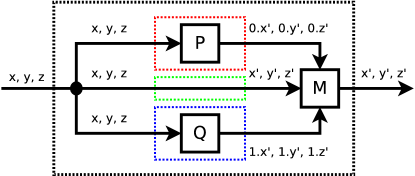
Figure 1: Parallel-by-merge Dataflow

The final operator we tackle in this section is parallel composition, written $P\mathop{\,{\mathrel{\parallel}}_{\hbox{\tiny\hbox{{{{R}}}}}}^{\text{\tiny$M$}}\,}Q$. Our definition of parallel composition, elaborated in Section 6.6, uses the parallel-by-merge scheme developed as part of UTP [33]. Since different concurrency schemes are possible for reactive contracts, depending on the underlying notion of trace, we cannot define a single parallel composition operator and so $P\mathop{\,{\mathrel{\parallel}}_{\hbox{\tiny\hbox{{{{R}}}}}}^{\text{\tiny$M$}}\,}Q$ is parametric over $M$. This is a merge predicate that defines how the state, traces, and any other observational variables should be merged following execution of $P$ and $Q$.

We illustrate parallel-by-merge in Figure 1, where we assume the programs act on three variables, $x$, $y$, and $z$. Parallel-by-merge splits the observation space into three identical segments: one for $P$, one for $Q$, and a third that is identical to the original input. Relation $M$ then takes the outputs from $P$, $Q$, and the original inputs, and merges them into a single output.

For reactive designs, the variables we need to merge are the state variables (st), trace (tt), and any additional observational variables $r$. As an example, we present below the merge predicate for interleaving the events of two Circus processes [33, 47].

Example 4.18 (Interleaving Merge).

$$M_{c}\,\,\,\triangleq\,\,\, \text{{tt}}\in(0.\text{{tt}}\mathrel{{|}\mkern-2.0mu{|}\mkern-2.0mu{|}}_{t}1.\text{{tt}})\mathrel{\wedge}ref^{\prime}\subseteq 0.\text{{ref}}\cap 1.\text{{ref}}\quad\mbox{where}$$

$$\langle\rangle\mathrel{{|}\mkern-2.0mu{|}\mkern-2.0mu{|}}_{t}xs\,\,\,=\,\,\, xs\mathrel{{|}\mkern-2.0mu{|}\mkern-2.0mu{|}}_{t}\langle\rangle\,\,\,=\,\,\,\{xs\}$$

$$\langle x\rangle\mathbin{\smash{\raise 3.44444pt\hbox{$\smallfrown$}}}xs\mathrel{{|}\mkern-2.0mu{|}\mkern-2.0mu{|}}_{t}\langle y\rangle\mathbin{\smash{\raise 3.44444pt\hbox{$\smallfrown$}}}ys\,\,\,=\,\,\, \left\{\langle x\rangle\mathbin{\smash{\raise 3.44444pt\hbox{$\smallfrown$}}}zs\,\,\middle|\,\,zs\in(xs\mathrel{{|}\mkern-2.0mu{|}\mkern-2.0mu{|}}_{t}\langle y\rangle\mathbin{\smash{\raise 3.44444pt\hbox{$\smallfrown$}}}ys)\right\}\,\cup\,$$

$$\left\{\langle y\rangle\mathbin{\smash{\raise 3.44444pt\hbox{$\smallfrown$}}}zs\,\,\middle|\,\,zs\in(\langle x\rangle\mathbin{\smash{\raise 3.44444pt\hbox{$\smallfrown$}}}xs\mathrel{{|}\mkern-2.0mu{|}\mkern-2.0mu{|}}_{t}ys)\right\}$$

$$P\mathrel{{|}\mkern-2.0mu{|}\mkern-2.0mu{|}}Q\,\,\,\triangleq\,\,\, P\mathop{\,{\mathrel{\parallel}}_{\hbox{\tiny\hbox{{{{R}}}}}}^{\text{\tiny$M_{c}$}}\,}Q$$

In the definition of $P\mathop{\,{\mathrel{\parallel}}_{\hbox{\tiny\hbox{{{{R}}}}}}^{\text{\tiny$M$}}\,}Q$, the trace and refusal variables are decorated with an index $0$ or $1$ that determine whether the quantity originates from $P$ or $Q$, respectively. The binary operator $\mathrel{{|}\mkern-2.0mu{|}\mkern-2.0mu{|}}_{t}$ interleaves two traces; it is a recursive function on sequences, returning a set of possible traces. The merge predicate, $M_{c}$, firstly constructs the overall trace tt as one of all possible interleavings, and secondly states that an event is only refused if it is refused by both processes. Our merge predicate leaves the state variable st unspecified as the Circus interleaving operator hides any internal state, since they can not in general be merge without further machinery for shared variables. We then define the interleaving operator $P\mathrel{{|}\mkern-2.0mu{|}\mkern-2.0mu{|}}Q$ using the parametric reactive design parallel composition operator $\mathop{\,{\mathrel{\parallel}}_{\hbox{\tiny\hbox{{{{R}}}}}}^{\text{\tiny$\cdot$}}\,}$, which is formally defined in Section 6.6. ∎

For the purpose of generic laws, we assume that any merge predicate yields well-formed traces, and furthermore is symmetric. Symmetry in this context means that the merge predicate has no bias towards either of its operands and yields the same result if they are swapped. This is clearly the case in Example 4.18, since both the traces and refusals are composed by symmetric operators, namely $\mathrel{{|}\mkern-2.0mu{|}\mkern-2.0mu{|}}_{t}$ and $\cap$. The following theorem describes the result of composing two contracts.

Theorem 4.19 (Reactive Design Parallel Composition).

$$\left[\,P_{1}\,\,\scalebox{0.5}[1.0]{$-$}\middle|\,\,\,P_{2}\,\,\middle|\,\,P_{3}\,\right]\mathop{\,{\mathrel{\parallel}}_{\hbox{\tiny\hbox{{{{R}}}}}}^{\text{\tiny$M$}}\,}\left[\,Q_{1}\,\,\scalebox{0.5}[1.0]{$-$}\middle|\,\,\,Q_{2}\,\,\middle|\,\,Q_{3}\,\right]=$$

$$\qquad\left[\,\begin{array}[]{l}(P_{1}\mathop{\mathrel{\Rightarrow}_{\!{\mbox{\tiny{r}}}}}P_{2})\mathop{\,\hbox{{{{wr}}}}_{\!\text{\tiny$M$}\,}}Q_{1}\mathrel{\wedge}\\ (P_{1}\mathop{\mathrel{\Rightarrow}_{\!{\mbox{\tiny{r}}}}}P_{3})\mathop{\,\hbox{{{{wr}}}}_{\!\text{\tiny$M$}\,}}Q_{1}\mathrel{\wedge}\\ (Q_{1}\mathop{\mathrel{\Rightarrow}_{\!{\mbox{\tiny{r}}}}}Q_{2})\mathop{\,\hbox{{{{wr}}}}_{\!\text{\tiny$M$}\,}}P_{1}\mathrel{\wedge}\\ (Q_{1}\mathop{\mathrel{\Rightarrow}_{\!{\mbox{\tiny{r}}}}}Q_{3})\mathop{\,\hbox{{{{wr}}}}_{\!\text{\tiny$M$}\,}}P_{1}\end{array}\,\,\scalebox{0.5}[1.0]{$-$}\middle|\,\,\,\begin{array}[]{l}P_{2}\mathop{\,{\mathrel{\parallel}}_{\hbox{\tiny\hbox{{{{E}}}}}}^{\text{\tiny$M$}}\,}Q_{2}\,\mathrel{\vee}\\[4.30554pt] P_{3}\mathop{\,{\mathrel{\parallel}}_{\hbox{\tiny\hbox{{{{E}}}}}}^{\text{\tiny$M$}}\,}Q_{2}\,\mathrel{\vee}\\[4.30554pt] P_{2}\mathop{\,{\mathrel{\parallel}}_{\hbox{\tiny\hbox{{{{E}}}}}}^{\text{\tiny$M$}}\,}Q_{3}\end{array}\,\,\middle|\,\,P_{3}\mathrel{\parallel}_{\text{\tiny$M$}}Q_{3}\,\right]$$

The precondition is expressed in terms of a reactive condition combinator $\mathop{\,\hbox{{{{wr}}}}_{\!\text{\tiny$M$}\,}}$. This is a form of weakest rely condition: $A\mathop{\,\hbox{{{{wr}}}}_{\!\text{\tiny$M$}\,}}B$ describes the weakest context in which reactive relation $A$ does not violate reactive condition $B$. This is necessary because in a composition like $P\mathop{\,{\mathrel{\parallel}}_{\hbox{\tiny\hbox{{{{R}}}}}}^{\text{\tiny$M$}}\,}Q$, the reactive processes $P$ and $Q$ interfere and this can lead to the violation of their preconditions. Thus, the overall precondition of a parallel composition itself assumes that such interferences do not occur. Interferences cannot occur in Example 4.18, since there is no synchronisation, but, in general, of course it can happen when more specialised merge predicates are employed. The definition of $\mathop{\,\hbox{{{{wr}}}}_{\!\text{\tiny$M$}\,}}$ is elided for now, as it requires further elaboration of the UTP theory, but is given in Section 6, Definition 6.26. It obeys several theorems that are shown below:

Theorem 4.20 (Weakest Rely Laws).

$$\hbox{{{{false}}}}\mathop{\,\hbox{{{{wr}}}}_{\!\text{\tiny$M$}\,}}P=\hbox{{{{true}}}}_{\mbox{\tiny{r}}}\qquad P\mathop{\,\hbox{{{{wr}}}}_{\!\text{\tiny$M$}\,}}\hbox{{{{true}}}}_{\mbox{\tiny{r}}}=\hbox{{{{true}}}}_{\mbox{\tiny{r}}}\qquad\left(\bigsqcap_{i\in I}\,P(i)\right)\mathop{\,\hbox{{{{wr}}}}_{\!\text{\tiny$M$}\,}}Q=\left(\bigwedge_{i\in I}\,(P(i)\mathop{\,\hbox{{{{wr}}}}_{\!\text{\tiny$M$}\,}}Q)\right)$$

The laws show, respectively, that (1) a miraculous reactive relation satisfies any precondition, (2) any reactive relation satisfies a true precondition, and (3) the weakest rely condition of a disjunction of relations is the conjunction of their weakest rely conditions.

The parallel composition precondition in Theorem 4.19 states that the respective preconditions of the two contracts, $P_{1}$ and $Q_{1}$, are not violated, neither by the opposing periconditions – respectively $Q_{2}$ and $P_{2}$ – under their respective preconditions, or the opposing postconditions – respectively $Q_{3}$ and $P_{3}$. The pericondition of the parallel reactive contract is written in terms of operator $P\mathop{\,{\mathrel{\parallel}}_{\hbox{\tiny\hbox{{{{E}}}}}}^{\text{\tiny$M$}}\,}Q$ that merges the traces but not the states, since this is concealed in intermediate observations. A parallel process is in an intermediate state if either of the composed processes is. Finally, the postcondition merges the final trace and state of each process, directly using the parallel by merge operator ($\mathrel{\parallel}_{M}$). We formally define all these operators in Section 6.6.

We can use Theorems 4.19 and 4.20 to prove the following theorem; for illustration we elaborate the complete calculation.

Theorem 4.21.

$\hbox{{{{Miracle}}}}\mathop{\,{\mathrel{\parallel}}_{\hbox{\tiny\hbox{{{{R}}}}}}^{\text{\tiny$M$}}\,}P=\hbox{{{{Miracle}}}}$

Proof.

$$\hbox{{{{Miracle}}}}\mathop{\,{\mathrel{\parallel}}_{\hbox{\tiny\hbox{{{{R}}}}}}^{\text{\tiny$M$}}\,}P =\left[\,\hbox{{{{true}}}}_{\mbox{\tiny{r}}}\,\,\scalebox{0.5}[1.0]{$-$}\middle|\,\,\,\hbox{{{{false}}}}\,\,\middle|\,\,\hbox{{{{false}}}}\,\right]\mathop{\,{\mathrel{\parallel}}_{\hbox{\tiny\hbox{{{{R}}}}}}^{\text{\tiny$M$}}\,}\left[\,P_{1}\,\,\scalebox{0.5}[1.0]{$-$}\middle|\,\,\,P_{2}\,\,\middle|\,\,P_{3}\,\right]$$

$$=\left[\,\begin{array}[]{l}(\hbox{{{{true}}}}_{\mbox{\tiny{r}}}\mathop{\mathrel{\Rightarrow}_{\!{\mbox{\tiny{r}}}}}\hbox{{{{false}}}})\mathop{\,\hbox{{{{wr}}}}_{\!\text{\tiny$M$}\,}}P_{1}\mathrel{\wedge}\\ (\hbox{{{{true}}}}_{\mbox{\tiny{r}}}\mathop{\mathrel{\Rightarrow}_{\!{\mbox{\tiny{r}}}}}\hbox{{{{false}}}})\mathop{\,\hbox{{{{wr}}}}_{\!\text{\tiny$M$}\,}}P_{1}\mathrel{\wedge}\\ (P_{1}\mathop{\mathrel{\Rightarrow}_{\!{\mbox{\tiny{r}}}}}P_{2})\mathop{\,\hbox{{{{wr}}}}_{\!\text{\tiny$M$}\,}}\hbox{{{{true}}}}_{\mbox{\tiny{r}}}\mathrel{\wedge}\\ (P_{1}\mathop{\mathrel{\Rightarrow}_{\!{\mbox{\tiny{r}}}}}P_{3})\mathop{\,\hbox{{{{wr}}}}_{\!\text{\tiny$M$}\,}}\hbox{{{{true}}}}_{\mbox{\tiny{r}}}\end{array}\,\,\scalebox{0.5}[1.0]{$-$}\middle|\,\,\,\begin{array}[]{l}\hbox{{{{false}}}}\mathop{\,{\mathrel{\parallel}}_{\hbox{\tiny\hbox{{{{E}}}}}}^{\text{\tiny$M$}}\,}P_{2}\,\mathrel{\vee}\\ \hbox{{{{false}}}}\mathop{\,{\mathrel{\parallel}}_{\hbox{\tiny\hbox{{{{E}}}}}}^{\text{\tiny$M$}}\,}P_{2}\,\mathrel{\vee}\\ \hbox{{{{false}}}}\mathop{\,{\mathrel{\parallel}}_{\hbox{\tiny\hbox{{{{E}}}}}}^{\text{\tiny$M$}}\,}P_{3}\end{array}\,\,\middle|\,\,\hbox{{{{false}}}}\mathrel{\parallel}_{\text{\tiny M}}P_{3}\,\right] [\ref{thm:rdespar}]$$

$$=\left[\,\begin{array}[]{l}\hbox{{{{false}}}}\mathop{\,\hbox{{{{wr}}}}_{\!\text{\tiny$M$}\,}}P_{1}\mathrel{\wedge}\hbox{{{{false}}}}\mathop{\,\hbox{{{{wr}}}}_{\!\text{\tiny$M$}\,}}P_{1}\mathrel{\wedge}\\ \hbox{{{{true}}}}_{\mbox{\tiny{r}}}\mathrel{\wedge}\hbox{{{{true}}}}_{\mbox{\tiny{r}}}\end{array}\,\,\scalebox{0.5}[1.0]{$-$}\middle|\,\,\,\begin{array}[]{l}\hbox{{{{false}}}}\,\mathrel{\vee}\,\hbox{{{{false}}}}\,\mathrel{\vee}\,\hbox{{{{false}}}}\end{array}\,\,\middle|\,\,\hbox{{{{false}}}}\,\right] [\ref{thm:wrlaws}]$$

$$=\left[\,\begin{array}[]{l}\hbox{{{{true}}}}_{\mbox{\tiny{r}}}\mathrel{\wedge}\hbox{{{{true}}}}_{\mbox{\tiny{r}}}\end{array}\,\,\scalebox{0.5}[1.0]{$-$}\middle|\,\,\,\begin{array}[]{l}\hbox{{{{false}}}}\end{array}\,\,\middle|\,\,\hbox{{{{false}}}}\,\right] [\ref{thm:wrlaws}]$$

$$=\left[\,\hbox{{{{true}}}}_{\mbox{\tiny{r}}}\,\,\scalebox{0.5}[1.0]{$-$}\middle|\,\,\,\hbox{{{{false}}}}\,\,\middle|\,\,\hbox{{{{false}}}}\,\right]$$

$$=\hbox{{{{Miracle}}}}$$

This law shows that composition of any predicate with a miracle always yields a miracle, regardless of the merge predicate. The intuitive property that Chaos is similarly an annihilator depends on the form of merge predicate, and so this cannot be proved in general. We perform a further example calculation using the interleaving operator from Example 4.18.

Example 4.22 (Interleaving Calculation).

$$\quad\,\,a\mathrel{\rightarrow}\hbox{{{{Skip}}}}\mathrel{{|}\mkern-2.0mu{|}\mkern-2.0mu{|}}b\mathrel{\rightarrow}\hbox{{{{Stop}}}}$$

$$=\left[\,\!\,\,\scalebox{0.5}[1.0]{$-$}\middle|\,\,\,a\notin\text{{ref}}^{\prime}\mathrel{\wedge}\text{{tt}}=\langle\rangle\,\,\middle|\,\,\text{{st}}^{\prime}=\text{{st}}\mathrel{\wedge}\text{{tt}}=\langle a\rangle\,\right]\mathrel{{|}\mkern-2.0mu{|}\mkern-2.0mu{|}}\left[\,\!\,\,\scalebox{0.5}[1.0]{$-$}\middle|\,\,\,a\notin\text{{ref}}^{\prime}\mathrel{\wedge}\text{{tt}}=\langle\rangle\mathrel{\vee}\text{{tt}}=\langle b\rangle\,\,\middle|\,\,\hbox{{{{false}}}}\,\right]$$

$$=\left[\,\!\,\,\scalebox{0.5}[1.0]{$-$}\middle|\,\,\,\begin{array}[]{l}(a\notin\text{{ref}}^{\prime}\mathrel{\wedge}\text{{tt}}=\langle\rangle)\mathop{\,{\mathrel{\parallel}}_{\hbox{\tiny\hbox{{{{E}}}}}}^{\text{\tiny$M_{C}$}}\,}(b\notin\text{{ref}}^{\prime}\mathrel{\wedge}\text{{tt}}=\langle\rangle)\mathrel{\vee}\\ (a\notin\text{{ref}}^{\prime}\mathrel{\wedge}\text{{tt}}=\langle\rangle)\mathop{\,{\mathrel{\parallel}}_{\hbox{\tiny\hbox{{{{E}}}}}}^{\text{\tiny$M_{C}$}}\,}(\text{{tt}}=\langle b\rangle)\mathrel{\vee}\\ (\text{{st}}^{\prime}=\text{{st}}\mathrel{\wedge}\text{{tt}}=\langle a\rangle)\mathop{\,{\mathrel{\parallel}}_{\hbox{\tiny\hbox{{{{E}}}}}}^{\text{\tiny$M_{C}$}}\,}(b\notin\text{{ref}}^{\prime}\mathrel{\wedge}\text{{tt}}=\langle\rangle)\mathrel{\vee}\\ (\text{{st}}^{\prime}=\text{{st}}\mathrel{\wedge}\text{{tt}}=\langle a\rangle)\mathop{\,{\mathrel{\parallel}}_{\hbox{\tiny\hbox{{{{E}}}}}}^{\text{\tiny$M_{C}$}}\,}(\text{{tt}}=\langle b\rangle)\end{array}\,\,\middle|\,\,(\text{{st}}^{\prime}=\text{{st}}\mathrel{\wedge}\text{{tt}}=\langle a\rangle)\mathrel{\parallel}_{\text{\tiny$M$}}\hbox{{{{false}}}}\,\right]$$

$$=\left[\,\!\,\,\scalebox{0.5}[1.0]{$-$}\middle|\,\,\,\begin{array}[]{l}(a\notin\text{{ref}}^{\prime}\mathrel{\wedge}b\notin\text{{ref}}^{\prime}\mathrel{\wedge}\text{{tt}}=\langle\rangle)\mathrel{\vee}\\ (a\notin\text{{ref}}^{\prime}\mathrel{\wedge}\text{{tt}}\in\{\langle\rangle,\langle b\rangle\})\mathrel{\vee}\\ (b\notin\text{{ref}}^{\prime}\mathrel{\wedge}\text{{tt}}\in\{\langle\rangle,\langle a\rangle\})\mathrel{\vee}\\ (\text{{tt}}=\langle a,b\rangle)\end{array}\,\,\middle|\,\,\hbox{{{{false}}}}\,\right]$$

$$=\left[\,\!\,\,\scalebox{0.5}[1.0]{$-$}\middle|\,\,\,(a\notin\text{{ref}}^{\prime}\mathrel{\wedge}b\notin\text{{ref}}^{\prime})\mathop{\hbox{\raisebox{0.0pt}{$\leftslice$}}}\text{{tt}}=\langle\rangle\mathop{\hbox{\raisebox{0.0pt}{$\rightslice$}}}\left(\begin{array}[]{l}a\notin\text{{ref}}^{\prime}\mathrel{\wedge}\text{{tt}}=\langle b\rangle\\ \mathrel{\vee}b\notin\text{{ref}}^{\prime}\mathrel{\wedge}\text{{tt}}=\langle a\rangle\\ \mathrel{\vee}\text{{tt}}=\langle a,b\rangle\end{array}\right)\,\,\middle|\,\,\hbox{{{{false}}}}\,\right]$$

$$=a\mathrel{\rightarrow}b\mathrel{\rightarrow}\hbox{{{{Stop}}}}\mathrel{\Box}b\mathrel{\rightarrow}a\mathrel{\rightarrow}\hbox{{{{Stop}}}}$$

We use the abbreviation $\left[\,\!\,\,\scalebox{0.5}[1.0]{$-$}\middle|\,\,\,P_{2}\,\,\middle|\,\,P_{3}\,\right]$ for a contract with a $\hbox{{{{true}}}}_{\mbox{\tiny{r}}}$ precondition. In the first step, we calculate the meaning of the two sequential processes using Examples 4.4 and 4.5, with Theorem 4.13. We then employ Theorem 4.19 to expand out the overall parallel reactive contract. There is no possibility of divergence, so the preconditions remain trivial. For the pericondition we need to merge each quiescent observation with every opposing quiescent or final observation. The result is the four conjuncts displayed. In the postcondition, we have to merge the two overall postconditions. The overall postcondition becomes false, because Stop prevents the overall operator from successfully terminating. In the pericondition, we calculate the four merged quiescent observations. These characterise the states when (1) no event has yet occurred, and we are accepting $a$ or $b$; (2) either $\langle\rangle$, or else $\langle b\rangle$ has occurred and $a$ remains enabled, which includes the situation when the right hand action has performed a transition; (3) the symmetric case to (2) with $a$ potentially having occurred; and (4) both events have occurred and no event is enabled: the refusal set is unconstrained. In common with the semantics of CSP[48], we observe that the set of possible refusals is downward closed under $\subseteq$ for every trace combination. We can then in fact show that this contract is equivalent to an external choice using the definition given in Example 4.6. ∎

This completes our exposition of the calculational laws for our reactive contract theory. All the theorems presented have been mechanically checked, as we discuss in Section 7. In the next section we illustrate their use in verification.

5 Automated Verification using Contracts

In this section, we exemplify the use of reactive contracts to verify properties of a small cash-card system described in Circus, using the verification procedure outlined in Section 4.1. We will explicitly calculate the implementation contracts, and show how these are then verified. Though the corresponding calculations are complex, the crucial detail is that they symbolically characterise reactive programs with potentially infinite state, and can be produced automatically in Isabelle/UTP.

In this example, cards can independently perform transfers to one another, provided sufficient balance exists. A key requirement is that there is no loss or increase of the value shared across the cards. For simplicity, we will construct a purely sequential specification of this system, and show how these properties can be discharged. We use a modified version of the model described in [62], which describes a network of a number of cards, each of which is identified by a natural number ${\mathbb{N}}$. Monetary amounts are represented as integers, ${\mathbb{Z}}$, so that we can additionally represent negative balances.

The central process has a single state variable $accts:{\mathbb{N}}\mathrel{\ooalign{\hfil$\mapstochar\mkern 5.0mu$\hfil\cr$\rightarrow$}}{\mathbb{Z}}$, a partial function that represents the set of accounts: the balance on each card. We also introduce three channels:

• $pay:{\mathbb{N}}\times{\mathbb{N}}\times{\mathbb{Z}}$, to initiate a transfer request of a given value between two cards;

• $reject:{\mathbb{N}}$, to indicate rejection of a transfer from the given card identifier;

• $accept:{\mathbb{N}}$, to indicate acceptance.

In order to update a particular account stored in $accts$, we need a form of assignment that applies to a single entry. We therefore introduce the following indexed assignment operator:

Definition 5.1 (Indexed Assignment).

$$x(i)\,\mathop{:=_{\textit{{\tiny C}}}}\,v\,\,\triangleq\,\,\left[\,i\in\mathop{\mathrm{dom}}(\text{{st}}.x)\,\,\scalebox{0.5}[1.0]{$-$}\middle|\,\,\,\hbox{{{{false}}}}\,\,\middle|\,\,\text{{st}}^{\prime}=\text{{st}}(x\mapsto x(i\mapsto v))\mathrel{\wedge}\text{{tt}}=\langle\rangle\,\right]$$

Indexed assignment $x(i)\,\mathop{:=_{\textit{{\tiny C}}}}\,v$, as employed by the $Pay$ action, is unlike regular assignment in that it is a partial operator and can only be executed when the collection $x$ has the index $i$ defined. Consequently, it must be guarded by an assumption $i\in\mathop{\mathrm{dom}}(\text{{st}}.x)$, which states that the index $i:A$ is in the domain of variable $x:A\mathrel{\ooalign{\hfil$\mapstochar\mkern 5.0mu$\hfil\cr$\rightarrow$}}B$.

We give indexed assignment a denotational semantics using a Circus contract, thus extending the available operators, which also illustrates the extensibility of our approach. The construct has similar semantics to regular assignment, but has the precondition that the given collection index must exist. The postcondition states that the collection state variable $x$ is updated so that the index $i$ maps to $v$. If the precondition is violated, then the result is divergence as the following calculation demonstrates:

Example 5.2 (Divergent Indexed Assignment).

$$\quad x\,\mathop{:=_{\hbox{\tiny\hbox{{{{R}}}}}}}\,\emptyset\mathrel{\hbox{\rm;}}x(i)\,\mathop{:=_{\textit{{\tiny C}}}}\,v$$

$$=\!\!\!\begin{array}[]{l}\left[\,\hbox{{{{true}}}}_{\mbox{\tiny{r}}}\,\,\scalebox{0.5}[1.0]{$-$}\middle|\,\,\,\hbox{{{{false}}}}\,\,\middle|\,\,\text{{st}}^{\prime}=\text{{st}}(x\mapsto\emptyset)\mathrel{\wedge}\text{{tt}}=\langle\rangle\,\right]\mathrel{\hbox{\rm;}}\\ \left[\,i\in\mathop{\mathrm{dom}}(\text{{st}}.x)\,\,\scalebox{0.5}[1.0]{$-$}\middle|\,\,\,\hbox{{{{false}}}}\,\,\middle|\,\,\text{{st}}^{\prime}=\text{{st}}(x\mapsto x(i\mapsto v))\mathrel{\wedge}\text{{tt}}=\langle\rangle\,\right]\end{array} [\ref{thm:rdescore},\ref{def:iassign}]$$

$$=\left[\,\hbox{{{{true}}}}_{\mbox{\tiny{r}}}\mathrel{\wedge}(\text{{st}}^{\prime}=\text{{st}}(x\mapsto\emptyset)\mathrel{\wedge}\text{{tt}}=\langle\rangle)\mathop{\,\hbox{{{{wlp}}}}_{r}\,}(i\in\mathop{\mathrm{dom}}(\text{{st}}.x))\,\,\scalebox{0.5}[1.0]{$-$}\middle|\,\,\,\hbox{{{{false}}}}\,\,\middle|\,\,\cdots\,\right] [\ref{thm:rdes-seq}]$$

$$=\left[\,i\in\mathop{\mathrm{dom}}(\emptyset)\,\,\scalebox{0.5}[1.0]{$-$}\middle|\,\,\,\hbox{{{{false}}}}\,\,\middle|\,\,\cdots\,\right] [\text{relational calculus}]$$

$$=\hbox{{{{Chaos}}}} [\ref{law:RD8}]$$

If we assign $\emptyset$, the empty partial function, to $x$ and then attempt to manipulate the $i$th element of $x$, the result is always Chaos. ∎

If we use an indexed assignment within a reactive program, then it is necessary to show that the applied indices are always in scope. We can now define the key actions for the cash card system.

Definition 5.3 (Card System).

$$Pay(i,j:{\mathbb{N}},n:{\mathbb{Z}})\,\,\triangleq\,\,\,\, pay.i.j.n\mathrel{\rightarrow}$$

$$\penalty 10000\ \,\left(\begin{array}[]{l}reject.i\mathrel{\rightarrow}\hbox{{{{Skip}}}}\\[4.30554pt] \quad\mathop{\hbox{\raisebox{0.0pt}{$\leftslice$}}}i=j\mathrel{\vee}i\notin\mathop{\mathrm{dom}}(accts)\mathrel{\vee}n\leq 0\mathrel{\vee}n>accts(i)\mathop{\hbox{\raisebox{0.0pt}{$\rightslice$}}}\\[4.30554pt] \left(\begin{array}[]{l}accts(i)\,\mathop{:=_{\textit{{\tiny C}}}}\,accts(i)-n\mathrel{\hbox{\rm;}}\\ accts(j)\,\mathop{:=_{\textit{{\tiny C}}}}\,accts(j)+n\mathrel{\hbox{\rm;}}\\ accept.i\mathrel{\rightarrow}\hbox{{{{Skip}}}}\end{array}\right)\end{array}\right)$$

$$PaySet(cs:\mathop{\mathstrut{\mathbb{P}}}\nolimits{\mathbb{N}})\,\,\triangleq\,\,\,\, \{(i:{\mathbb{N}},j:{\mathbb{N}},n:{\mathbb{Z}})|i\in cs\mathrel{\wedge}j\in cs\mathrel{\wedge}i\neq j\}$$

$$SomePay(cs:\mathop{\mathstrut{\mathbb{P}}}\nolimits{\mathbb{N}})\,\,\triangleq\,\,\,\, \bigsqcap(i,j,n)\in PaySet(cs)@Pay(i,j,n)$$

$$Cycle(cs:\mathop{\mathstrut{\mathbb{P}}}\nolimits{\mathbb{N}})\,\,\triangleq\,\,\,\, \mathop{\mathstrut{\mu}}\nolimits X@SomePay(cs)\mathrel{\hbox{\rm;}}X$$

$$System\,\,\triangleq\,\,\,\, accts\,\mathop{:=_{\textit{{\tiny C}}}}\,\langle 100,100,100,100,100\rangle\mathrel{\hbox{\rm;}}Cycle(\{0..4\})$$

Action $Pay(i,j,n)$ defines the protocol to execute a payment request between cards $i$ and $j$ of amount $n$. If $i=j$, and thus the cards are the same, or card $i$ does not exist, then the transfer is rejected, by offering $reject.i$ and then terminating. Likewise, if there is insufficient balance or a negative transfer is requested, then the transfer is also rejected. If the transfer can be performed, then two indexed assignments lower the balance of card $i$ and raise the balance of card $j$, respectively. Finally, the $accept.i$ event is offered and then the action terminates.

The main behaviour of the system is described by the $Cycle$ action, which takes the set of card identifiers $cs:\mathop{\mathstrut{\mathbb{P}}}\nolimits{\mathbb{N}}$ as a parameter. It iterates the action $SomePay(cs)$, which consists of an internal choice over all possible payments between all possible cards, $PaySet(cs)$. The behaviour of an example card system is described by the action $System$ that creates 5 cards, each with a balance of 100, and then begins the cycle.

In order to verify properties of the processes, we first need to calculate the reactive design contract of the system. For the purposes of illustration, we focus on the $Pay$ action. The other contracts can be calculated in terms of the $Pay$ contract using the laws presented in Section 4. The following theorem provides the result of the calculation. Like all other theorems in this paper, it is proved, not by hand, but by use of our tactics in Isabelle/UTP.

Theorem 5.4 (Pay Action Contract Calculation).

$Pay(i,j,n)=\left[\,P_{1}\,\,\scalebox{0.5}[1.0]{$-$}\middle|\,\,\,P_{2}\,\,\middle|\,\,P_{3}\,\right]$ where

$$P_{1}=\,\,\,\, \langle pay.i.j.n\rangle\leq\text{{tt}}\mathrel{\wedge}i\neq j\mathrel{\wedge}i\notin\mathop{\mathrm{dom}}(accts)\mathrel{\wedge}0<n\mathrel{\wedge}n<accts(i)$$

$$\mathrel{\Rightarrow}\,\,\,\, j\in\mathop{\mathrm{dom}}(accts)$$

$$P_{2}=\,\,\,\, \text{{tt}}=\langle\rangle\mathrel{\wedge}pay.i.j.n\notin\text{{ref}}^{\prime}$$

$$\mathrel{\vee}\,\,\,\, \text{{tt}}=\langle pay.i.j.n\rangle\mathrel{\wedge}(i=j\mathrel{\vee}n<0\mathrel{\vee}n>accts(i))\mathrel{\wedge}reject.i\notin\text{{ref}}^{\prime}$$

$$\mathrel{\vee}\,\,\,\, \text{{tt}}=\langle pay.i.j.n\rangle\mathrel{\wedge}i\neq j\mathrel{\wedge}n<0\mathrel{\wedge}n>accts(i)\mathrel{\wedge}accept.i\notin\text{{ref}}^{\prime}$$

$$P_{3}=\,\,\,\, \text{{tt}}=\langle pay.i.j.n,reject.i\rangle\mathrel{\wedge}(i=j\mathrel{\vee}n<0\mathrel{\vee}n>accts(i))\mathrel{\wedge}\text{{st}}^{\prime}=\text{{st}}$$

$$\mathrel{\vee}\,\,\,\, \text{{tt}}=\langle pay.i.j.n,accept.i\rangle\mathrel{\wedge}i\neq j\mathrel{\wedge}n<0\mathrel{\wedge}n>accts(i)$$

$$\qquad\mathrel{\wedge}accts:=accts(i\mapsto accts(i)-n,j\mapsto accts(j)+n)$$

Theorem 5.4 gives the result of the calculation of the precondition $P_{1}$, pericondition $P_{2}$, and postcondition $P_{3}$ of the implementation contract for the $Pay$ action. Intuitively, this complex contract symbolically characterises the potentially infinite state space and possible transitions that the $Pay$ action can make, depending on the initial state. The precondition specifies the circumstances under which behaviour is predictable, the pericondition specifies the possible quiescent observation, and the postcondition specifies the terminating observations.

Precondition $P_{1}$ requires that, if the $pay.i.j.n$ event occurs, that is, it is at the head of the trace, and the conditions for a valid transfer are all satisfied by the state, then it must be the case that card $j$ exists in the state space. This precondition arises directly from the indexed assignment: its violation leads to unpredictable behaviour. Thus, if the transfer is not offered or the payment is not valid then this assignment is not reached, and so the precondition precisely identifies the state in which divergence is possible. We alternatively could remove this precondition altogether by altering the definition of $Pay$ so that if $j\notin\mathop{\mathrm{dom}}(accts)$ then also a $reject$ event is issued. However, for illustration purposes we leave the precondition in place. This precondition is a reactive condition because it only restricts a prefix of the trace to the left of the implication and only refers to initial state variables.

The pericondition, $P_{2}$, specifies the three possible intermediate observations for the action. Firstly, we have the scenario in which nothing has happened yet, so the trace is empty and the $pay.i.j.n$ is being offered – it is not being refused. Secondly, it is possible that the transfer request occurred, and so the trace has a singleton event, but one of the conditions for a valid transfer is violated, and thus the $reject.i$ event is being offered. Thirdly, we can have that a valid transfer request occurred and so the $accept.i$ event is being offered. At this point the state update has happened internally, but it cannot yet be observed as the action is still in an intermediate state.

The postcondition, $P_{3}$, specifies two possible final states, one for an invalid transfer request, in which case the state remains the same, and one for a valid transfer, in which case the two balances are updated. In both cases the trace is updated with two events, and no refusals are recorded since we have terminated.

The next step in verification is to specify some holistic properties of our system that we would like to show. We chose three properties: (1) there is no increase or decrease in the overall balance across cards, (2) no overdrafts on the card balances are permitted, and (3) if a valid transfer request is made it must be executed. It is not difficult to see that these properties hold, but the purpose is to show how they can specified and verified using reactive contracts.

Each of these properties is assigned a contract which $Pay(i,j,n)$ must refine. We therefore demonstrate the three properties as three corresponding theorems, which have been discharged in Isabelle/UTP using the rdes-refine tactic (see Section 7), which employs Theorem 4.2 and the contract calculation laws. For the purpose of illustration, we give high-level informal proofs that correspond to the mechanised proofs.

Theorem 5.5 (No Increase or Decrease in Value).

A payment between card $i$ and $j$, where $\{i,j\}\subseteq cs$ and $i\neq j$, does not lead to an overall change in balance for the system of cards. Formally, as a reactive contract:

$$\left[\,\mathop{\mathrm{dom}}(accts)=cs\,\,\scalebox{0.5}[1.0]{$-$}\middle|\,\,\,\hbox{{{{true}}}}_{\mbox{\tiny{r}}}\,\,\middle|\,\,sum(accts)=sum(accts^{\prime})\,\right]\mathrel{\sqsubseteq}Pay(i,j,n)$$

where $sum$ is a function that sums up the range of the given partial function. We set the pericondition $\hbox{{{{true}}}}_{\mbox{\tiny{r}}}$ as we do not need to constrain quiescent states in this specification.

Proof.

We first apply Theorem 4.2 to split the refinement into three proof obligations. We need to show that the precondition is weakened, and the peri- and postconditions are strengthened, which we tackle one at a time:

1. $\mathop{\mathrm{dom}}(accts)=cs\mathrel{\Rightarrow}P_{1}$

2. $P_{2}\mathrel{\wedge}\mathop{\mathrm{dom}}(accts)=cs\mathrel{\Rightarrow}\hbox{{{{true}}}}_{\mbox{\tiny{r}}}$

3. $P_{3}\mathrel{\wedge}\mathop{\mathrm{dom}}(accts)=cs\mathrel{\Rightarrow}sum(accts)=sum(accts^{\prime})$

Case (1) follows because $i,j\in cs$ and since the domain of $accts$ is $cs$, then clearly both $i,j\in\mathop{\mathrm{dom}}(accts)$. Case (2) follows trivially. Case (3) requires that we consider both cases of postcondition $P_{3}$. If the payment request is invalid, then $accts^{\prime}=accts$ since $\text{{st}}^{\prime}=\text{{st}}$, and thus clearly $sum(accts)=sum(accts^{\prime})$. If the payment request is valid, then we need to show that $sum(accts)=sum(accts(i\mapsto accts(i)-n,j\mapsto accts(j)+n))$. This is equal to $sum(accts)-n+n=sum(accts)$, and so we are done. ∎

Theorem 5.6 (No overdrafts).

No card $i$ is permitted to have a negative balance:

$$\left[\,\mathop{\mathrm{dom}}(accts)=cs\,\,\scalebox{0.5}[1.0]{$-$}\middle|\,\,\,\hbox{{{{true}}}}_{\mbox{\tiny{r}}}\,\,\middle|\,\,\mathop{\mathstrut{\forall}}\nolimits k\in cs@accts(k)\geq 0\mathrel{\Rightarrow}accts^{\prime}(k)\geq 0\,\right]\mathrel{\sqsubseteq}Pay(i,j,n)$$

Proof.

The argument for the pre and periconditions is the same as in the previous theorem. For the postcondition we need to show that after a valid payment the balance of any valid card $k$ is not less than 0, that is, $accts(k)\geq 0$. The key property to prove here is $(accts(i\mapsto accts(i)-n,j\mapsto accts(j)+n))(k)\geq 0$. We can do this by case analysis: $k=i$, $k=j$, and $k\neq i\mathrel{\wedge}k\neq j$. In the former two cases, the fact that the transfer happens indicates that the balances following must be no less than zero. In the final case, the balance remains the same, and so we are done. ∎

Theorem 5.7 (Transfer Acceptance).

If a payment is initiated and we have enough money in the account, then the transfer is not rejected:

$$\left[\,\mathop{\mathrm{dom}}(accts)=cs\,\,\scalebox{0.5}[1.0]{$-$}\middle|\,\,\,\begin{array}[]{c}\text{{tt}}\neq\langle\rangle\mathrel{\wedge}last(\text{{tt}})=pay.i.j.k\mathrel{\wedge}\\ n\leq accts(i)\mathrel{\Rightarrow}accept.i\notin ref^{\prime}\end{array}\,\,\middle|\,\,\hbox{{{{true}}}}_{\mbox{\tiny{r}}}\,\right]$$

Proof.

This property is different as it involves the pericondition rather than the postcondition. This is because we are reasoning about offered events in intermediate observations. We need to show in the pericondition that if the last event to occur is $pay.i.j.n$, and a sufficient amount is in account $i$ then we must not refuse to the accept the payment. This can be achieved by case analysis on pericondition $P_{2}$. ∎

Thus we have shown how our design contracts can be used to verify properties of simple Circus actions. In the next section we explore the UTP theory’s healthiness conditions behind our contracts — which provides support for this verification.

6 Theory of Generalised Reactive Designs

In this section, we present our UTP theory of reactive design contracts in detail. We describe the healthiness conditions, core signature definitions, and algebraic laws, which substantiate those given in Section 4. In particular, we define healthiness conditions for two UTP theories: SRD in Section 6.2, which is a recasting of the previous reactive design theory from [46], and NSRD in Section 6.3, a novel healthiness condition that refines SRD with additional constraints to support reactive preconditions and invisible intermediate states. This latter healthiness condition is the foundation of our reactive contract theory. We consider the algebraic law this theory supports, and the restrictions it places on expressible operators. In Section 6.5, we consider the formalisation of recursion, and show how Kleene’s fixed-point theorem [39] can be applied to calculate tail recursive reactive designs. Finally in Section 6.6, we detail our results in the formalisation of parallel composition.

6.1 UTP Theory Preliminaries

The theorems presented in Section 4, present reactive contracts using the syntactic form of $\left[\,P_{1}\,\,\scalebox{0.5}[1.0]{$-$}\middle|\,\,\,P_{2}\,\,\middle|\,\,P_{3}\,\right]$. It is often inconvenient to rely on such a specific syntactic form to reason about contracts, for example when stating algebraic theorems. It is much more convenient to a reactive contract $P$ as a relation that admits certain properties. Consequently, as usual in the UTP approach, we define healthiness conditions that characterise well-formed contract predicates. This allows us to obtain a large number of algebraic laws from lattice theory and related domains, and also allows us to reason about contracts without the need for the syntactic form.

In order to reason about contracts as opaque relations, we need a way of extracting the three parts from a contract. We therefore define the following three functions:

Definition 6.1 (Pre-, Peri-, and Postcondition Extraction Functions).

$$pre_{\hbox{\tiny\hbox{{{{R}}}}}}(P) \penalty 10000\ \,\triangleq\,\,\neg_{\mbox{\tiny{r}}}\,P[true,false,false/ok,ok^{\prime},wait]$$

$$peri_{\hbox{\tiny\hbox{{{{R}}}}}}(P) \penalty 10000\ \,\triangleq\,\,P[true,true,false,true/ok,ok^{\prime},wait,wait^{\prime}]$$

$$post_{\hbox{\tiny\hbox{{{{R}}}}}}(P) \penalty 10000\ \,\triangleq\,\,P[true,true,false,false/ok,ok^{\prime},wait,wait^{\prime}]$$

These three functions variously substitute the observational variables to obtain the respective characteristic predicates. In order to illustrate this, we first expand out the definition of reactive contract from Definition 4.1, and also using Definitions 2.6 and 2.10:

$$\left[\,P_{1}\,\,\scalebox{0.5}[1.0]{$-$}\middle|\,\,\,P_{2}\,\,\middle|\,\,P_{3}\,\right]=\hbox{{{{R1}}}}(\hbox{{{{R2}}}}_{c}({\hbox{{I \kern-8.5ptI}}}_{\!{\hbox{\tiny\hbox{{{{R}}}}}}}\mathop{\hbox{\raisebox{0.0pt}{$\leftslice$}}}wait\mathop{\hbox{\raisebox{0.0pt}{$\rightslice$}}}((ok\mathrel{\wedge}P_{1})\mathrel{\Rightarrow}(ok^{\prime}\mathrel{\wedge}(P_{2}\mathop{\hbox{\raisebox{0.0pt}{$\leftslice$}}}wait^{\prime}\mathop{\hbox{\raisebox{0.0pt}{$\rightslice$}}}P_{3})))))$$

From this, we can see that the crucial variables that dictate the various behaviours are $wait$, $ok$, $ok^{\prime}$, and $wait^{\prime}$. Variable $wait$ flags whether a sequential predecessor is in an intermediate state or has terminated, $ok$ flags whether a predecessor diverged, and $ok^{\prime}$ and $wait^{\prime}$ record this information for the present relation.

The precondition ($P_{1}$) is false when a reactive design was started ($ok\mathrel{\wedge}\neg wait$) but it diverged ($\neg ok^{\prime}$). Thus, to extract the precondition we set $ok$, $ok^{\prime}$, and $wait$ to $true$, $false$, and $false$, respectively, and negate the result using reactive negation. The pericondition is reached when the reactive design was started and did not diverge ($ok^{\prime}$), but has not yet reached its final state ($\neg wait^{\prime}$), and is thus intermediate. The postcondition is similarly obtained, but $wait^{\prime}$ becomes $false$. With these definitions we can prove theorems that allow us to extract the constituent reactive relations from a syntactic reactive contract.

Theorem 6.2 (Extracting Pre, Peri, and Postconditions).

$$pre_{\hbox{\tiny\hbox{{{{R}}}}}}(\left[\,P_{1}\,\,\scalebox{0.5}[1.0]{$-$}\middle|\,\,\,P_{2}\,\,\middle|\,\,P_{3}\,\right]) \penalty 10000\ \,=\,\,P_{1}$$

$$peri_{\hbox{\tiny\hbox{{{{R}}}}}}(\left[\,P_{1}\,\,\scalebox{0.5}[1.0]{$-$}\middle|\,\,\,P_{2}\,\,\middle|\,\,P_{3}\,\right]) \penalty 10000\ \,=\,\,P_{1}\mathop{\mathrel{\Rightarrow}_{\!{\mbox{\tiny{r}}}}}P_{2}$$

$$post_{\hbox{\tiny\hbox{{{{R}}}}}}(\left[\,P_{1}\,\,\scalebox{0.5}[1.0]{$-$}\middle|\,\,\,P_{2}\,\,\middle|\,\,P_{3}\,\right]) \penalty 10000\ \,=\,\,P_{1}\mathop{\mathrel{\Rightarrow}_{\!{\mbox{\tiny{r}}}}}P_{3}$$

Provided $P_{1}$, $Q_{1}$, and $Q_{2}$ are all RR healthy.

The pericondition and postcondition are viewed through the prism of the precondition being satisfied, which is why the implications are present in the result above. This is an important assumption of reactive designs. Although it is possible to specify behaviours in the peri and postcondition outside the precondition, once the contract is constructed these behaviours are pruned, so that the behaviour of a contract when its precondition is violated is always Chaos.

6.2 Stateful Reactive Designs

In this section, we introduce the first of our two reactive design theories: stateful reactive designs. Motivated by the previous work on CSP and Circus in UTP [33, 10, 46], we define the following healthiness conditions for our generalised theory of reactive designs. We generalise the previous works [33, 10, 46] due to the underlying abstract trace algebra, and the extensible alphabet of our theory [16].

Definition 6.3 (Stateful Reactive Designs Healthiness Conditions).

$$\hbox{{{{RD1}}}}(P) \penalty 10000\ \,\triangleq\,\,ok\mathop{\mathrel{\Rightarrow}_{\!{\mbox{\tiny{r}}}}}P$$

$$\hbox{{{{RD2}}}}(P) \penalty 10000\ \,\triangleq\,\,P\mathrel{\hbox{\rm;}}\hbox{{{{J}}}}$$

$$\hbox{{{{SRD}}}}(P) \penalty 10000\ \,\triangleq\,\,\hbox{{{{RD1}}}}\mathrel{\circ}\hbox{{{{RD2}}}}\mathrel{\circ}\hbox{{{{R}}}}_{s}$$

RD1 and RD2 are analogous to H1 and H2 from the theory of designs. Moreover, RD1 and RD2 correspond to CSP1 and CSP2 from the theories of CSP [33, 10] and Circus [46]. We rename them, firstly because our theory has a different alphabet founded upon our trace algebra, and secondly because we do not specify the corresponding CSP3 and CSP4, which constrain $ref$ and are thus specific to CSP and Circus.

RD1 states, like H1, that observations are possible only after initiation, indicated by $ok$. However, unlike H1, if $ok$ is false the resulting predicate is not true, but $\hbox{{{{true}}}}_{\mbox{\tiny{r}}}$; that is, the trace must monotonically increase, but the behaviour is otherwise unpredictable. RD2 is identical to H2 and thus also CSP2.

Our overall healthiness condition for stateful reactive designs is then called SRD, which includes RD1, RD2, and $\hbox{{{{R}}}}_{s}$. Like RD1 and RD2, it is a generalisation of the overall Circus healthiness condition CSP [46]. We can next prove that SRD relations admit a certain syntactic formulation using reactive contracts, as shown in the following theorem.

Theorem 6.4 (Stateful Reactive Design Formulation).

$$\hbox{{{{SRD}}}}(P) =\left[\,pre_{\hbox{\tiny\hbox{{{{R}}}}}}(P)\,\,\scalebox{0.5}[1.0]{$-$}\middle|\,\,\,peri_{\hbox{\tiny\hbox{{{{R}}}}}}(P)\,\,\middle|\,\,post_{\hbox{\tiny\hbox{{{{R}}}}}}(P)\,\right]$$

If a relation is SRD healthy, then it takes the form of a reactive contract with a pre-, peri-, and postcondition. Theorem 6.4 thus allows us to take an SRD predicate and deconstruct it into its three parts, using the functions defined in Definition 6.1, which can then be manipulated separately. This theorem shows an equivalence between the syntactic formulation, and elements of $\llbracket\hbox{{{{SRD}}}}\rrbracket_{\mbox{\tiny{{H}}}}$: any element of the latter can be constructed using the contract triple notation. Conversely, a well-formed reactive design triple always yields a healthy reactive design. This is confirmed by the following closure theorem, which is a corollary of Theorems 6.4 and 6.2.

Corollary 6.4.1.

If $P_{1}$, $P_{2}$, and $P_{3}$ are all RR healthy then $\left[\,P_{1}\,\,\scalebox{0.5}[1.0]{$-$}\middle|\,\,\,P_{2}\,\,\middle|\,\,P_{3}\,\right]$ is SRD healthy.

In order to show that a reactive contract is SRD, it suffices to show that its pre-, peri-, and postcondition are all RR. A further corollary is the three triple extraction functions all produce healthy reactive relations when applied to an SRD relation.

Corollary 6.4.2.

If $P\mathop{\,\textit{is}\,}\hbox{{{{SRD}}}}$ then $pre_{\hbox{\tiny\hbox{{{{R}}}}}}(P)$, $peri_{\hbox{\tiny\hbox{{{{R}}}}}}(P)$, and $post_{\hbox{\tiny\hbox{{{{R}}}}}}(P)$ are all RR-healthy.

Having defined a candidate theory for our reactive contracts, we will now explore its algebraic properties. The class of SRD relations admits a number of useful identities that we outline below.

Theorem 6.5 (SRD Laws).

If $P$ is SRD healthy then

$${\hbox{{I \kern-8.5ptI}}}_{\!{\hbox{\tiny\hbox{{{{R}}}}}}}\mathrel{\hbox{\rm;}}P\,\,=\,\, P$$ (6.5.1)

$$\hbox{{{{Chaos}}}}\mathrel{\hbox{\rm;}}P\,\,=\,\,$$ Chaos (6.5.2)

$$\hbox{{{{Miracle}}}}\mathrel{\hbox{\rm;}}P\,\,=\,\,$$ Miracle (6.5.3)

${\hbox{{I \kern-8.5ptI}}}_{\!{\hbox{\tiny\hbox{{{{R}}}}}}}$ is a left unit of any SRD relation, and Chaos and Miracle are both left annihilators. However, in general ${\hbox{{I \kern-8.5ptI}}}_{\!{\hbox{\tiny\hbox{{{{R}}}}}}}$ is not a right unit, which the following theorem illustrates.

Theorem 6.6.

If $P_{1}$, $P_{2}$, and $P_{3}$ are RR then $\left[\,\!P_{1}\!\,\,\scalebox{0.5}[1.0]{$-$}\middle|\,\,\,\!P_{2}\!\,\,\middle|\,\,\!P_{3}\!\,\right]\mathrel{\hbox{\rm;}}{\hbox{{I \kern-8.5ptI}}}_{\!{\hbox{\tiny\hbox{{{{R}}}}}}}=\left[\,\neg_{\mbox{\tiny{r}}}\,(\neg_{\mbox{\tiny{r}}}\,P_{1})\mathrel{\hbox{\rm;}}\hbox{{{{true}}}}_{\mbox{\tiny{r}}}\,\,\scalebox{0.5}[1.0]{$-$}\middle|\,\,\,\mathop{\mathstrut{\exists}}\nolimits\text{{st}}^{\prime}@P_{2}\,\,\middle|\,\,P_{3}\,\right]$

Right composition with ${\hbox{{I \kern-8.5ptI}}}_{\!{\hbox{\tiny\hbox{{{{R}}}}}}}$ effectively imposes two additional requirements on the reactive contract: (1) that the negated precondition does not refer to dashed variables other than $tr^{\prime}$, which must be extension closed — it is RC1 (cf. Definition 3.9); and (2) that the pericondition does not refer to $\text{{st}}^{\prime}$, as characterised by the existential quantifier. The latter follows as a direct consequence of $\hbox{{{{R3}}}}_{h}$ [7] (cf. Definition 2.10), which requires that st must not be restricted in an intermediate state. Thus, composition of $P$ with ${\hbox{{I \kern-8.5ptI}}}_{\!{\hbox{\tiny\hbox{{{{R}}}}}}}$ has the same effect on $\text{{st}}^{\prime}$ in $P$ since ${\hbox{{I \kern-8.5ptI}}}_{\!{\hbox{\tiny\hbox{{{{R}}}}}}}$ ignores any intermediate states ($wait^{\prime}=true$), rather than passing them forward to a successor process.

The former restriction is a direct consequence of healthiness condition RD1. To explain why, we consider the reactive design $P\mathrel{\hbox{\rm;}}{\hbox{{I \kern-8.5ptI}}}_{\!{\hbox{\tiny\hbox{{{{R}}}}}}}$ in the situation when $P$ has started ($ok\mathrel{\wedge}wait$), but diverged ($\neg ok^{\prime}$). The following calculation shows the result.

Example 6.7 (Divergence and RD1).

$$\quad\,(P\mathrel{\wedge}ok\mathrel{\wedge}\neg ok^{\prime}\mathrel{\wedge}\neg wait)\mathrel{\hbox{\rm;}}{\hbox{{I \kern-8.5ptI}}}_{\!{\hbox{\tiny\hbox{{{{R}}}}}}}$$

$$=P[true,false,false/ok,ok^{\prime},wait^{\prime}]\mathrel{\hbox{\rm;}}{\hbox{{I \kern-8.5ptI}}}_{\!{\hbox{\tiny\hbox{{{{R}}}}}}}[false/ok]$$ [relational calculus]

$$=(\neg_{\mbox{\tiny{r}}}\,pre_{\hbox{\tiny\hbox{{{{R}}}}}}(P))\mathrel{\hbox{\rm;}}{\hbox{{I \kern-8.5ptI}}}_{\!{\hbox{\tiny\hbox{{{{R}}}}}}}[false/ok]$$ [Definition 6.1]

$$=(\neg_{\mbox{\tiny{r}}}\,pre_{\hbox{\tiny\hbox{{{{R}}}}}}(P))\mathrel{\hbox{\rm;}}(\hbox{{{{RD1}}}}({\hbox{{I \kern-8.5ptI}}}_{\!{\hbox{\tiny\hbox{{{{R}}}}}}}))[false/ok]$$ [Theorem 6.4.1]

$$=(\neg_{\mbox{\tiny{r}}}\,pre_{\hbox{\tiny\hbox{{{{R}}}}}}(P))\mathrel{\hbox{\rm;}}(ok\mathop{\mathrel{\Rightarrow}_{\!{\mbox{\tiny{r}}}}}{\hbox{{I \kern-8.5ptI}}}_{\!{\hbox{\tiny\hbox{{{{R}}}}}}})[false/ok]$$ [Definition 6.3]

$$=(\neg_{\mbox{\tiny{r}}}\,pre_{\hbox{\tiny\hbox{{{{R}}}}}}(P))\mathrel{\hbox{\rm;}}\hbox{{{{true}}}}_{\mbox{\tiny{r}}}$$ [predicate calculus]

When $P$ diverges with $\neg ok^{\prime}$, its behaviour is $\neg_{\mbox{\tiny{r}}}\,pre_{\hbox{\tiny\hbox{{{{R}}}}}}(P)$: the precondition has been violated. Moreover, if $ok^{\prime}$ is false in $P$ then $ok$ is false in ${\hbox{{I \kern-8.5ptI}}}_{\!{\hbox{\tiny\hbox{{{{R}}}}}}}$, which yields the relation $\hbox{{{{true}}}}_{\mbox{\tiny{r}}}$. Actually, this follows for any RD1 relation, not just ${\hbox{{I \kern-8.5ptI}}}_{\!{\hbox{\tiny\hbox{{{{R}}}}}}}$, since $\hbox{{{{RD1}}}}[false/ok]=\hbox{{{{true}}}}_{\mbox{\tiny{r}}}$. Consequently, right composition with any SRD relation yields the same result: the precondition should be RC1.

Consequently, the right composition law motivates that we need to consider a refined theory for reactive contracts, in order to support the desirable algebraic and calculational laws of Section 4. This is the objective of the following section.

6.3 Normal Stateful Reactive Designs

We refine SRD by identifying the subclass of normal stateful reactive designs, NSRD, which provides the theory domain of our reactive contracts.

Definition 6.8 (Normal Stateful Reactive Designs Healthiness Conditions).

$$\hbox{{{{RD3}}}}(P) \penalty 10000\ \,\triangleq\,\,P\mathrel{\hbox{\rm;}}{\hbox{{I \kern-8.5ptI}}}_{\!{\hbox{\tiny\hbox{{{{R}}}}}}}$$

$$\hbox{{{{NSRD}}}}(P) \penalty 10000\ \,\triangleq\,\,\hbox{{{{RD1}}}}\mathrel{\circ}\hbox{{{{RD3}}}}\mathrel{\circ}\hbox{{{{R}}}}_{s}$$

RD3 is analogous to H3: it requires that skip is a right unit. This ensures that the precondition is a reactive condition and the pericondition does not depend on $\text{{st}}^{\prime}$. The use of the word “normal” here is therefore by analogy with normal designs [21]. NSRD does not explicitly invoke RD2 as it is subsumed by RD3, as the following theorem demonstrates.

Theorem 6.9 (RD3 subsumes RD2).

$\hbox{{{{RD2}}}}(\hbox{{{{RD3}}}}(P))=\hbox{{{{RD3}}}}(\hbox{{{{RD2}}}}(P))=\hbox{{{{RD3}}}}(P)$

Proof.

This follows since $\hbox{{{{J}}}}\mathrel{\hbox{\rm;}}{\hbox{{I \kern-8.5ptI}}}_{\!{\hbox{\tiny\hbox{{{{R}}}}}}}={\hbox{{I \kern-8.5ptI}}}_{\!{\hbox{\tiny\hbox{{{{R}}}}}}}\mathrel{\hbox{\rm;}}\hbox{{{{J}}}}={\hbox{{I \kern-8.5ptI}}}_{\!{\hbox{\tiny\hbox{{{{R}}}}}}}$. ∎

Consequently, it is easy to show that every NSRD-healthy relation is also SRD-healthy, and therefore the theorems of Section 6.2 remain valid. We can also prove the following theorem that follows as a consequence of Theorems 6.9 and 6.6.

Theorem 6.10 (Normal Stateful Reactive Design Formulation).

$$\hbox{{{{NSRD}}}}(P) =\left[\,\hbox{{{{RC1}}}}(pre_{\hbox{\tiny\hbox{{{{R}}}}}}(P))\,\,\scalebox{0.5}[1.0]{$-$}\middle|\,\,\,(\mathop{\mathstrut{\exists}}\nolimits\text{{st}}^{\prime}@peri_{\hbox{\tiny\hbox{{{{R}}}}}}(P))\,\,\middle|\,\,post_{\hbox{\tiny\hbox{{{{R}}}}}}(P)\,\right]$$

In addition to ensuring that the elements of the triple of RR healthy, NSRD also ensures that the precondition is a reactive condition, and that the pericondition does not refer to $\text{{st}}^{\prime}$.

Corollary 6.10.1.

$P$ is NSRD healthy provided that the following conditions hold:

1. $P$ is SRD healthy;

2. $pre_{\hbox{\tiny\hbox{{{{R}}}}}}(P)$ is RC healthy;

3. $peri_{\hbox{\tiny\hbox{{{{R}}}}}}(P)$ does not mention $\text{{st}}^{\prime}$.

A further corollary finally justifies the syntactic formulation given in Section 4:

Corollary 6.10.2 (NSRD contract closure).

If $P_{1}$ is RC, $P_{2}$ and $P_{3}$ are both RR, and $P_{2}$ does not refer to $\text{{st}}^{\prime}$, then $\left[\,P_{1}\,\,\scalebox{0.5}[1.0]{$-$}\middle|\,\,\,P_{2}\,\,\middle|\,\,P_{3}\,\right]$ is NSRD healthy.

We now, therefore, have an adequate formulation of the reactive design theory. In spite of its restrictions, SRD remains useful as a means of obtaining algebraic theorems. In the remainder of this section we will therefore explore the algebraic properties of the two theories.

6.4 Algebraic Properties

SRD and NSRD are both idempotent and continuous, and therefore both form complete lattices, as stated in the following theorem.

Theorem 6.11 (Reactive Design Lattices).

SRD and NSRD healthy predicates form complete lattices with $\top_{\hbox{\tiny\hbox{{{{R}}}}}}\triangleq\hbox{{{{SRD}}}}(\hbox{{{{false}}}})=\hbox{{{{Miracle}}}}$ and $\bot_{\hbox{\tiny\hbox{{{{R}}}}}}\triangleq\hbox{{{{SRD}}}}(\hbox{{{{true}}}})=\hbox{{{{Chaos}}}}$.

Proof.

Standard proofs of idempotency for CSP1 and CSP2 [33, 10] apply also to RD1 and RD2, respectively. RD3 is idempotent since ${\hbox{{I \kern-8.5ptI}}}_{\!{\hbox{\tiny\hbox{{{{R}}}}}}}\mathrel{\hbox{\rm;}}{\hbox{{I \kern-8.5ptI}}}_{\!{\hbox{\tiny\hbox{{{{R}}}}}}}={\hbox{{I \kern-8.5ptI}}}_{\!{\hbox{\tiny\hbox{{{{R}}}}}}}$. RD1 is continuous since it is disjunctive. RD2 and RD3 are both continuous since sequential composition distributes through infima to the left and right. ∎

We note that both Miracle and Chaos, following the form given in Theorem 6.10.2, are both NSRD healthy. Through the Knaster-Tarski theorem [55], we also obtain weakest fixed-point operators $\mathop{\mathstrut{\mu}}\nolimits\!\!_{\hbox{\tiny\hbox{{{{R}}}}}}$ and $\mathop{\mathstrut{\mu}}\nolimits\!\!_{\hbox{\tiny\hbox{{{{N}}}}}}$ for the two theories, which we will further explore in Section 6.5. Since SRD and NSRD are also continuous, by Theorem 2.5 we can rewrite the weakest fixed-points to $\mathop{\mathstrut{\mu}}\nolimits X@F(\hbox{{{{SRD}}}}(X))$ and $\mathop{\mathstrut{\mu}}\nolimits X@F(\hbox{{{{NSRD}}}}(X))$, respectively. Thus, we can reason about recursive reactive designs using the relational calculus lattice rather than the theory specific ones. We can also show that reactive designs are closed under the standard relational calculus operators, as the following theorems demonstrate.

Theorem 6.12 (Reactive Design Composition).

If $P$ and $Q$ are NSRD healthy then

$$P\mathrel{\hbox{\rm;}}Q=\hbox{{{{R}}}}_{s}\left(\begin{array}[]{l}pre_{\hbox{\tiny\hbox{{{{R}}}}}}(P)\mathrel{\wedge}(post_{\hbox{\tiny\hbox{{{{R}}}}}}(P)\mathop{\,\hbox{{{{wlp}}}}_{r}\,}pre_{\hbox{\tiny\hbox{{{{R}}}}}}(Q))\\[2.15277pt] \mathrel{\vdash}\,\,peri_{\hbox{\tiny\hbox{{{{R}}}}}}(P)\mathrel{\vee}(post_{\hbox{\tiny\hbox{{{{R}}}}}}(P)\mathrel{\hbox{\rm;}}peri_{\hbox{\tiny\hbox{{{{R}}}}}}(Q))\\[2.15277pt] \mathop{\,\,\diamond\,\,}\,\,post_{\hbox{\tiny\hbox{{{{R}}}}}}(P)\mathrel{\hbox{\rm;}}post_{\hbox{\tiny\hbox{{{{R}}}}}}(Q)\end{array}\right)$$

Theorem 6.12 is essentially the same as Theorem 4.13.24, but relies on healthiness of $P$ and $Q$, rather than their syntactic form. As similar law holds for SRD-healthy predicates, though with a more complex precondition and pericondition, following the form given in Theorem 6.6. We finally show closure of the theory under the main programming operators.

Theorem 6.13 (Reactive Designs Closure).

SRD and NSRD healthy predicates are closed under $\mathrel{\sqcap}$, $\sqcup$, $\mathop{\hbox{\raisebox{0.0pt}{$\leftslice$}}}b\mathop{\hbox{\raisebox{0.0pt}{$\rightslice$}}}$,  $\mathrel{\hbox{\rm;}}$ , ${\hbox{{I \kern-8.5ptI}}}_{\!{\hbox{\tiny\hbox{{{{R}}}}}}}$, $\langle\sigma\rangle_{\hbox{\tiny\hbox{{{{R}}}}}}$, Miracle, and Chaos.

This closure theorem means that we can import the algebraic laws for the relational calculus operators from core UTP [33], such as several equations of Theorem 2.3. Finally, we note that our theory admits the following familiar laws from relational calculus for assignment.

Theorem 6.14 (Reactive Design Assignment Compositions).

If $P$ is NSRD healthy, $x$ is a state variable, and $v$ is an expression containing only state variables, then:

$$(x\,\mathop{:=_{\hbox{\tiny\hbox{{{{R}}}}}}}\,v)\,\mathrel{\hbox{\rm;}}\,P\,\,=\,\, P[v/x]$$ (6.14.1)

$$\langle\sigma\rangle_{\hbox{\tiny\hbox{{{{R}}}}}}\,\mathrel{\hbox{\rm;}}\,P\,\,=\,\, \sigma\mathop{\dagger}P$$ (6.14.2)

Theorem 6.14.1, the more usual law [32], shows that a sequential assignment can be turned into a substitution applied to its successor. It is an instance of the more general Theorem 6.14.2 when $\sigma=\{x\mapsto v\}$, crucially, provided that $x$ is a state variable and not an arbitrary UTP variable.

Theorem 6.14 depends directly on the use of $\hbox{{{{R3}}}}_{h}$, and the resulting requirement that periconditions do not refer to after state. It would not hold if allowed such references, for example by substituting $\hbox{{{{R3}}}}_{h}$ with the original healthiness condition R3 [33]. In order to understand why, consider the following corollary of Theorem 6.14.1 involving a Circus event prefix:

Theorem 6.15 (Assignment and Events).

$$(x\,\mathop{:=_{\hbox{\tiny\hbox{{{{R}}}}}}}\,e\mathrel{\hbox{\rm;}}c\mathrel{\rightarrow}P)\,\,=\,\,(c[e/x]\mathrel{\rightarrow}(x\,\mathop{:=_{\hbox{\tiny\hbox{{{{R}}}}}}}\,e\mathrel{\hbox{\rm;}}P))$$

Theorem 6.15 allows us to push assignment through event prefixes, whilst making an appropriate substitution. It can be found in reactive languages like Occam [49]. This law does not hold in previous Circus semantics [46] as $\text{{st}}^{\prime}$ (there called $v^{\prime}$) is revealed in intermediate states. Thus, whilst the left hand side of this equation admits an intermediate observation where $x$ is updated to $e$, because the pericondition does characterise state updates, the right hand side does not.

There are, however, costs to this simplification. A side effect is to prevent encoding of McEwan’s Circus interruption operator [40], which has the form $P\mathop{\triangle_{i}}Q$. This operator is similar to $P\mathrel{{|}\mkern-2.0mu{|}\mkern-2.0mu{|}}(i\mathrel{\rightarrow}Q)$, except that if the interruption event $i$ occurs before $P$ terminates, and whilst it is quiescent, then the remaining behaviour of $P$ is pruned. If $P$ terminates, then conversely the behaviours of $Q$ are lost. Crucially, the internal state of $P$ is retained following interruption [7], and is passed on to $Q$, which is unique to McEwan’s work (cf. [53, 58, 60]). For example, consider the following action:

$$(x:=5\mathrel{\hbox{\rm;}}a\mathrel{\rightarrow}\hbox{{{{Skip}}}})\mathop{\triangle_{b}}\,(x:=x+x).$$

First, we note that the leading assignment $x:=5$ cannot be interrupted, since it does not have a quiescent state. However, once this has occurred the left-hand side enters a quiescent state where $a$ is enabled. Through the interruption operator, $b$ is also enabled at this point. If $a$ occurs then the entire action terminates in a final state with $x=5$. However, if $b$ occurs then the value of $x$ at this point is retained, and the action $x:=x+x$ occurs, leading to final value of $10$ for $x$.

We see, therefore, how the value of $x$ is retained and used by the interruption action. Such a retention of the state, however, cannot be represented in the presence of RD3 as no intermediate state variables are recorded. Therefore, if such an interruption operator is required, the loss of Theorem 6.15 must be accepted, and R3 used as the base of reactive designs instead. This is a design choice depending on the kind of reasoning and expressivity needed, as R3 reactive designs carry more information and so are more distinguishing than $\hbox{{{{R3}}}}_{h}$ reactive designs. R3 is supported in Isabelle/UTP if its use is desired.

6.5 Recursion

In this section we will show how to calculate reactive contracts for a restricted class of recursive models, with the particular aim of substantiating Theorem 4.15. In Section 6.4, we have shown that generalised reactive designs form a complete lattice. Thus, for any monotonic process constructor $F$ we can be sure there exists fixed-points $\mathop{\mathstrut{\mu}}\nolimits\!\!_{\hbox{\tiny\hbox{{{{R}}}}}}\,F$ and $\nu\!\!_{\hbox{\tiny\hbox{{{{R}}}}}}\,F$. However, in order to reason about recursive reactive contracts generally, we need to calculate the pre, peri, and postconditions of such constructions.

In general, we are most interested in the weakest fixed-point for reactive designs, $\mathop{\mathstrut{\mu}}\nolimits\!\!_{\hbox{\tiny\hbox{{{{R}}}}}}\,F$, as the strongest fixed-point yields miraculous behaviour for erroneous constructions [9]. For example, $(\nu\!\!_{\hbox{\tiny\hbox{{{{R}}}}}}\,X@X)=\hbox{{{{Miracle}}}}$, whereas in reality an infinite loop is a programmer error that should yield Chaos, which $\mathop{\mathstrut{\mu}}\nolimits\!\!_{\hbox{\tiny\hbox{{{{R}}}}}}\,X@X$ does.

In order to calculate the reactive design of a weakest fixed-point we employ two results: (1) Hoare and He’s proof that guarded processes yield unique fixed-points [33, theorem 8.1.13, page 206], and (2) Kleene’s fixed-point theorem [39]. The latter allows us to convert from a recursive construction with a strongest fixed-point to an iterative construction, using a replicated internal choice of power constructions. Since we can calculate the reactive design of replicated processes, we can therefore tackle recursion.

Hoare and He’s theorem states, informally, that guarded functions on reactive processes have a unique fixed-point, that is, if, for any relation $X$, $F(X)$ is guarded, then $\mathop{\mathstrut{\mu}}\nolimits F=\nu F$. Guardedness is defined as follows.

Definition 6.16 (Guarded Reactive Designs).

A function on reactive designs $F:\llbracket\hbox{{{{SRD}}}}\rrbracket_{\mbox{\tiny{{H}}}}\to\llbracket\hbox{{{{SRD}}}}\rrbracket_{\mbox{\tiny{{H}}}}$ is guarded provided that, for any $P\in\llbracket\hbox{{{{SRD}}}}\rrbracket_{\mbox{\tiny{{H}}}}$ and $n\in\mathbb{N}$,

$$(F(P)\mathrel{\wedge}gv(n+1))=(F(P\mathrel{\wedge}gv(n))\mathrel{\wedge}gv(n+1))$$

where $gv(n)\triangleq(tr\leq tr^{\prime}\mathrel{\wedge}\#\text{{tt}}<n)$ and $\#:\mathcal{T}\to\mathbb{N}$ is a discrete trace measure function. We extend the trace algebra $(\mathcal{T},\mathop{\,\,\widehat{}\,\,},\varepsilon)$ with the following axioms for the measure function; for $s,t\in\mathcal{T}$:

$$\#\varepsilon=0\qquad s>0\mathrel{\Rightarrow}\#s>\varepsilon\qquad\#(s\mathop{\,\,\widehat{}\,\,}t)=\#s+\#t$$

Definition 6.16 is similar to the one given in [33], but is generalised to allow a variety of different discrete measure functions that satisfy the measure function axioms. An example measure function that satisfies these axioms is the length function on sequences.

Given a reactive design $\mathop{\mathstrut{\mu}}\nolimits X@F(X)$, if $F$ is guarded according to Definition 6.16 then, intuitively, before recursion variable $X$ can be reached, $F$ must have produced a non-empty portion of the trace. For example, in CSP we may have a process $\mathop{\mathstrut{\mu}}\nolimits X@a\mathrel{\rightarrow}X$, which is guarded since it must perform an $a$ before recursing. This is ensured by requiring that the trace contribution of the function applied to a reactive design $F(P)$ yields a trace strictly longer than that produced by $P$. This is the purpose of $gv$: if we observe $F(P)$ in a context where the trace is longer than $n+1$ (enforced by $gv(n+1)$) then we can conclude that the trace contributed by $P$ must be no longer than $n$, and thus we can conjoin it with $gv(n)$. We can use this to prove Hoare and He’s theorem.

Theorem 6.17 (Unique Fixed-Points).

If $F$ is guarded then $\mathop{\mathstrut{\mu}}\nolimits F=\nu F$.

Technically, the $\mathop{\mathstrut{\mu}}\nolimits$ and $\nu$ operators we use here are those of the relational calculus lattice, and not of an arbitrary UTP theory (hence the lack of subscripts). The proof given in [33, theorem 8.1.13, page 206], which our mechanised proof follows, omits the step that transitions the theory fixed-point operator ($\mathop{\mathstrut{\mu}}\nolimits\!\!_{\hbox{\tiny\hbox{{{{R}}}}}}$) to the relational one ($\mathop{\mathstrut{\mu}}\nolimits$). However, this step is necessary in order to employ their approximation chain theorem [33, theorem 2.7.6, page 63]. Thus, in order to employ Theorem 6.17 for reactive designs, we first have to use Theorems 6.11 and 2.5 to convert the reactive design fixed-point operator. Continuity of SRD is thus an important property. Using that, for any guarded process, we can convert a recursive construction using a weakest fixed-point to one using a strongest fixed-point.

In order to make use of Theorem 6.17, it is necessary to prove guardedness theorems for the operators of the target language. In general, this can be quite complicated; in many cases, however, we can shortcut guardedness and instead focus on tail-recursive fixed-point constructions of the form $\mathop{\mathstrut{\mu}}\nolimits\!\!_{\hbox{\tiny\hbox{{{{R}}}}}}\,X@P\mathrel{\hbox{\rm;}}X$, where $X$ is not mentioned in $P$, as employed by Theorem 4.15. This pattern, though restrictive, covers a large number of specifiable Circus processes, for instance. In this case, guardedness can be shown simply by showing that $P$ always produces events before it terminates. Of course, $P$ may not terminate at all, but in this case the recursion variable $X$ is unreachable and thus $\mathop{\mathstrut{\mu}}\nolimits\!\!_{\hbox{\tiny\hbox{{{{R}}}}}}\,X@P\mathrel{\hbox{\rm;}}X$ reduces to $P$. Whether or not $P$ terminates, productivity is the criterion needed (see Definition 4.14), and from this we can prove the following theorem.

Theorem 6.18.

If $P$ is productive then the function $\mathop{\mathstrut{\lambda}}\nolimits X@P\mathrel{\hbox{\rm;}}X$ is guarded.

So, by Theorem 6.17 we can map the weakest fixed-point to the strongest fixed-point. This brings us to Kleene’s fixed-point theorem, which allows us to calculate an iterative construction for the strongest fixed-point of a continuous function.

Theorem 6.19 (Kleene’s fixed-point theorem).

If $F$ is a continuous function then the strongest fixed-point can be calculated by iteration:

$$\nu F\,\,=\,\,\bigsqcap_{i\in{\mathbb{N}}}F^{i}(\hbox{{{{false}}}})$$

Kleene’s fixed-point theorem often employs Scott-continuity as its antecedent, which is based on complete partial orders rather than complete lattices. We employ our stronger notion of continuity in Theorem 6.19, since we do have a complete lattice in our setting. Theorem 6.19 allows us to calculate the fixed-point by iterating $F$, starting from false, which is the top ($\top$) of the relational lattice. Now, for our simplified pattern $\nu X@P\mathrel{\hbox{\rm;}}X$ we automatically have continuity since relational composition is continuous, that is

$$(\bigsqcap i@P(i))\mathrel{\hbox{\rm;}}Q=(\bigsqcap i@P(i)\mathrel{\hbox{\rm;}}Q)$$

is a theorem of relational calculus (see Theorem 2.3). Combining this property with Theorem 4.13.25, which includes the calculation for a power construction, we are now in the position to substantiate Theorem 4.15 for calculating iterative reactive contracts. We give the calculational proof below explicitly since it uses and illustrates several of our results.

Proof of Theorem 4.15.

$$\quad\,\mathop{\mathstrut{\mu}}\nolimits\!\!_{\hbox{\tiny\hbox{{{{R}}}}}}\,X@\left[\,P\,\,\scalebox{0.5}[1.0]{$-$}\middle|\,\,\,Q\,\,\middle|\,\,R\,\right]\mathrel{\hbox{\rm;}}X$$

$$=\mathop{\mathstrut{\mu}}\nolimits X@\left[\,P\,\,\scalebox{0.5}[1.0]{$-$}\middle|\,\,\,Q\,\,\middle|\,\,R\,\right]\mathrel{\hbox{\rm;}}\hbox{{{{SRD}}}}(X)$$ [Theorem 2.5.6]

$$=\nu X@\left[\,P\,\,\scalebox{0.5}[1.0]{$-$}\middle|\,\,\,Q\,\,\middle|\,\,R\,\right]\mathrel{\hbox{\rm;}}\hbox{{{{SRD}}}}(X)$$ [Theorems 6.17 and 6.18]

$$=\bigsqcap_{i\in{\mathbb{N}}}(\mathop{\mathstrut{\lambda}}\nolimits X@\left[\,P\,\,\scalebox{0.5}[1.0]{$-$}\middle|\,\,\,Q\,\,\middle|\,\,R\,\right]\mathrel{\hbox{\rm;}}\hbox{{{{SRD}}}}(X))^{i}(\hbox{{{{false}}}})$$ [Theorem 6.19]

$$=\bigsqcap_{i\in{\mathbb{N}}}(\mathop{\mathstrut{\lambda}}\nolimits X@\left[\,P\,\,\scalebox{0.5}[1.0]{$-$}\middle|\,\,\,Q\,\,\middle|\,\,R\,\right]\mathrel{\hbox{\rm;}}\hbox{{{{SRD}}}}(X))^{i+1}(\hbox{{{{false}}}}) f^{0}(\hbox{{{{false}}}})=\hbox{{{{false}}}})$$ [Unfold: ]

$$=\bigsqcap_{i\in{\mathbb{N}}}(\left[\,P\,\,\scalebox{0.5}[1.0]{$-$}\middle|\,\,\,Q\,\,\middle|\,\,R\,\right]^{i+1}\mathrel{\hbox{\rm;}}\hbox{{{{SRD}}}}(\hbox{{{{false}}}})) i$$ [Induction on ]

$$=\bigsqcap_{i\in{\mathbb{N}}}(\left[\,P\,\,\scalebox{0.5}[1.0]{$-$}\middle|\,\,\,Q\,\,\middle|\,\,R\,\right]^{i+1}\mathrel{\hbox{\rm;}}\hbox{{{{Miracle}}}})$$ [Theorem 2.5.2]

$$=\bigsqcap_{i\in{\mathbb{N}}}\left[\,\bigwedge_{i\leq n}\left(R^{i}\mathop{\,\hbox{{{{wlp}}}}_{r}\,}P\right)\,\,\scalebox{0.5}[1.0]{$-$}\middle|\,\,\,\bigvee_{i\leq n}R^{i}\mathrel{\hbox{\rm;}}Q\,\,\middle|\,\,R^{n+1}\,\right]\mathrel{\hbox{\rm;}}\hbox{{{{Miracle}}}}$$ [Theorem 4.13.25]

$$=\bigsqcap_{i\in{\mathbb{N}}}\left[\,\bigwedge_{i\leq n}\left(R^{i}\mathop{\,\hbox{{{{wlp}}}}_{r}\,}P\right)\,\,\scalebox{0.5}[1.0]{$-$}\middle|\,\,\,\bigvee_{i\leq n}R^{i}\mathrel{\hbox{\rm;}}Q\,\,\middle|\,\,\hbox{{{{false}}}}\,\right]$$ [Theorem RD9]

$$=\left[\,\bigwedge_{i\in{\mathbb{N}}}\left(R^{i}\mathop{\,\hbox{{{{wlp}}}}_{r}\,}P\right)\,\,\scalebox{0.5}[1.0]{$-$}\middle|\,\,\,\bigvee_{i\in{\mathbb{N}}}R^{i}\mathrel{\hbox{\rm;}}Q\,\,\middle|\,\,\hbox{{{{false}}}}\,\right] \left[\begin{array}[]{r}\text{Theorem\penalty 10000\ \ref{thm:rdes-comp-inf} and}\\ \text{relational calculus}\end{array}\right]$$

This proof demonstrates the necessity of a large corpus of theorems we have proved from the UTP theories and reactive designs in order to reason about recursion. We now have a complete constructive approach for calculating the reactive contract for a variety of recursive specifications. Extension to deal with mutual recursion is laborious, but not challenging.

6.6 Parallel Composition

In this section we introduce the parametric parallel composition operator for reactive designs, and substantiate a number of preliminary results for the operator, including well-formedness conditions supported by a novel healthiness condition. Parallel composition in UTP is expressed in terms of the parallel-by-merge scheme $P\mathop{\mathrel{\parallel}_{M}}Q$, whereby the final states of concurrent separated processes $P$ and $Q$ are merged by predicate $M$. We adopt a slightly simplified definition of parallel-by-merge, originally presented in [19], which assumes that the alphabet of both $P$ and $Q$ is the same, but is otherwise semantically equivalent to the standard UTP definition [33, chapter 7].

Definition 6.20 (Parallel-by-Merge).

$$P\mathrel{\parallel}_{M}Q\,\triangleq\,(\lceil P\rceil_{0}\mathrel{\wedge}\lceil Q\rceil_{1}\mathrel{\wedge}v^{\prime}=v)\mathrel{\hbox{\rm;}}M$$

The intuition for parallel-by-merge is given in Figure 1. It splits the state space into three parts, one of which is passed to $P$, the second to $Q$, and the third is simply copied from the original input state. Assuming both $P$ and $Q$ produce an output, the merge predicate $M$ computes the overall output that should be given by merging the three states. For imperative programs, a simple example merge predicate may pick two disjoint subsets of the variables output by $P$ and $Q$ to produce an overall output. The value of such a scheme for parallel composition is that different concurrency schemes can be supported, and properties of the parallel composition operator often reduce to properties of the merge predicate [33, theorem 7.2.10, page 173].

To formalise this in Definition 6.20, we require that $P$ and $Q$ are homogeneous relations with the alphabet $\{v,v^{\prime}\}$, where $v$ is a vector of variables. $\lceil P\rceil_{0}$ and $\lceil Q\rceil_{1}$ rename the dashed variables by adding indices $0$ and $1$, respectively, so they can be distinguished by the merge predicate $M$. $M$ is a heterogeneous alphabetised relation whose alphabet is $\{0.v,1.v,v,v^{\prime}\}$. It takes three copies of the variables: the renamed dashed variables of $P$ and $Q$, and all undashed variables. The separated processes are conjoined, which is acceptable because of their disjoint output alphabets, along with a predicate that copies all initial variables ($v^{\prime}=v$). The resulting conjunctive relation is then composed in sequence with $M$. This merge predicate calculates the overall final state in terms of the initial state, and final states of $P$ and $Q$. Thus, the overall composition $P\mathrel{\parallel}_{M}Q$ has alphabet $\{v,v^{\prime}\}$.

For our theory of reactive designs, the objective, as indicated by Section 4.4 is to specialise parallel-by-merge so that it acts only on the trace, state, and other semantic observational variables (like ref). We therefore define the parametric merge predicate $\mathcal{M}_{R}(M)$ that merges $ok$ and $wait$ variables, so handling divergence and intermediate observations. It defers merging of the states and traces to an “inner merge predicate” $M$, such as $M_{c}$ described in Example 4.18. We require that $M$ does not refer to $ok$ or $wait$ nor decorations thereof.

We define three auxiliary merge operators that construct the “outer merge predicate”, by showing how $ok$ and $wait$ are merged, and imposition the reactive design healthiness conditions. These operators are then used to define the reactive design parallel composition operator.

Definition 6.21 (Reactive Designs Parallel Composition).

$$\mathcal{N}_{0}(M) \penalty 10000\ \triangleq\,(wait^{\prime}=(0.wait\mathrel{\vee}1.wait)\mathrel{\wedge}tr\leq tr^{\prime}\mathrel{\wedge}M)$$

$$\mathcal{N}_{1}(M) \penalty 10000\ \triangleq\,(ok^{\prime}=(0.ok\mathrel{\wedge}1.ok)\mathrel{\wedge}\mathcal{N}_{0}(M))$$

$$\mathcal{M}_{R}(M) \penalty 10000\ \triangleq\,\hbox{{{{RD3}}}}(\hbox{{{{RD1}}}}(\hbox{{{{R3}}}}_{h}(\mathcal{N}_{1}(M))))$$

$$P\mathop{\,{\mathrel{\parallel}}_{\hbox{\tiny\hbox{{{{R}}}}}}^{\text{\tiny$M$}}\,}Q \penalty 10000\ \triangleq\,P\mathrel{\parallel}_{\mathcal{M}_{R}(M)}Q$$

The auxiliary merge functions $\mathcal{N}_{0}$ and $\mathcal{N}_{1}$ conjoin the inner merge predicate $M$ with three conjuncts. $\mathcal{N}_{0}$ handles merging of the $wait$ variables. If either $P$ or $Q$ admits an intermediate observation ($0.wait$ or $1.wait$), then also the composite observation is intermediate, and thus we take the disjunction of the $wait$ variables to determine $wait^{\prime}$. The third conjunct ensures the resulting merge is R1 healthy. $\mathcal{N}_{1}$ handles merging of the $ok$ variables. If either $P$ or $Q$ diverges, then we require that their composition also diverges and thus $ok^{\prime}$ takes the conjunction of both $ok$ variables. Using $\mathcal{N}_{1}$, we then define the overall merge predicate $\mathcal{M}_{R}$ by application of three healthiness conditions to construct a stateful reactive design. The parametric merge of two reactive designs, $P\mathop{\,{\mathrel{\parallel}}_{\hbox{\tiny\hbox{{{{R}}}}}}^{\text{\tiny$M$}}\,}Q$ with inner merge predicate $M$, is simply a parallel-by-merge using $\mathcal{M}_{R}(M)$.

It remains to prove that NSRD is closed under reactive design parallel composition. In order to prove this, we need to restrict the form of the merge predicate using new healthiness conditions. Firstly, we need a modified version of $\hbox{{{{R2}}}}_{c}$ that is applicable to merge predicates, first defined in [16].

Definition 6.22 ($\hbox{{{{R2}}}}_{c}$ for Merge Predicates).

$$\hbox{{{{R2}}}}_{m}(M) \triangleq(P[\varepsilon,tr^{\prime}\!-\!tr,0.tr\!-\!tr,1.tr\!-\!tr/tr,tr^{\prime},0.tr,1.tr])\mathop{\hbox{\raisebox{0.0pt}{$\leftslice$}}}tr\leq tr^{\prime}\mathop{\hbox{\raisebox{0.0pt}{$\rightslice$}}}P$$

Merge predicates have three ways of accessing the trace history through the three respective copies of the trace variable. Thus, it is necessary to delete the history in $0.tr$, $1.tr$, and $tr$ in the healthiness condition $\hbox{{{{R2}}}}_{m}$ to ensure that this does not occur. This allows us to prove the following theorem

Theorem 6.23.

$P\mathrel{\parallel}_{M}Q$ is R1 and $\hbox{{{{R2}}}}_{c}$ healthy provided that $P$ and $Q$ are both R1 and $\hbox{{{{R2}}}}_{c}$, and $M$ is R1 and $\hbox{{{{R2}}}}_{m}$.

This theorem provides the circumstances under which a parallel-by-merge constructs a healthy reactive process. From this, we define the following healthiness condition for reactive-design inner merge predicates.

Definition 6.24 (Healthy Inner Merge Predicate).

$$\hbox{{{{RDM}}}}(M)\triangleq\hbox{{{{R2}}}}_{m}(\mathop{\mathstrut{\exists}}\nolimits 0.ok,1.ok,ok,ok^{\prime},0.wait,1.wait,wait,wait^{\prime}@M)$$

RDM contains $\hbox{{{{R2}}}}_{m}$ and additionally formalises the requirement that the inner merge predicate does not contain $ok$, $wait$, and decorations thereof, through existential quantification. These variables have already been handled by the outer merge predicate, and so the inner merge predicate should not refer to them. $M_{c}$ in Example 4.18 is clearly RDM, for example, since it refers only to $0.\text{{tt}}$ and $1.\text{{tt}}$, thus satisfying $\hbox{{{{R2}}}}_{m}$, and does not mention $ok$ or $wait$ in any way.

Using this definition of healthy reactive inner merges, we can then prove the following closure theorem for parallel composition:

Theorem 6.25 (Parallel Composition Closure).

If $P$ and $Q$ are SRD healthy, and $M$ is RDM healthy, then $P\mathrel{\parallel}_{M}Q$ is NSRD healthy.

As seen in Definition 6.21, parallel composition, like sequential composition, is not defined explicitly as a reactive design using the contract syntax. However, in order to calculate the meaning of a parallel reactive program it is necessary to know how to calculate a contract form for it. By Theorem 6.25 we know that parallel composition is a normal stateful reactive design (NSRD), and therefore we can invoke Theorem 6.10 to split it into a reactive design triple, toward substantiation of Theorem 4.19. It then suffices to calculate its pre-, peri-, and postcondition. In order to do this, we need to characterise interference between parallel processes using a notion of weakest rely condition. This is the weakest context under which two parallel composed processes do not violate one another’s assumptions.

Definition 6.26 (Weakest Rely Condition).

$$P\mathop{\,\hbox{{{{wr}}}}_{\!\text{\tiny$M$}\,}}Q\,\,\triangleq\,\, \neg_{\mbox{\tiny{r}}}\,((\neg_{\mbox{\tiny{r}}}\,Q)\mathrel{\parallel}_{\hbox{\small$M$}\mathrel{\hbox{\rm;}}\hbox{{{{true}}}}_{\mbox{\tiny{r}}}}P)$$

The operator $P\mathop{\,\hbox{{{{wr}}}}_{\!\text{\tiny$M$}\,}}Q$ is essentially the concurrent case of the reactive weakest precondition $\mathop{\,\hbox{{{{wlp}}}}_{r}\,}$ (cf. Definition 3.15). It represents the weakest context where reactive relation $P$ does not lead to the violation of reactive condition $Q$. We achieve this by first merging the possible traces of negated $Q$ with those of $P$ using the merge predicate $M$ composed with $\hbox{{{{true}}}}_{\mbox{\tiny{r}}}$. This determines all the behaviours permitted by merge predicate $M$ that are enabled by $P$ and yet violate $Q$. The composition with $\hbox{{{{true}}}}_{\mbox{\tiny{r}}}$ ensures that resulting reactive relation is extension closed. We then negate the resulting relation to obtain the overall reactive precondition.

We can show that the weakest rely condition constructor forms a reactive condition, which is essential to our using it in the reactive contract precondition:

Theorem 6.27 (Weakest Rely Condition forms a Reactive Condition).

If $P$ and $Q$ are RR healthy, and $M$ is RDM healthy, then $P\mathop{\,\hbox{{{{wr}}}}_{\!\text{\tiny$M$}\,}}Q$ is a reactive condition.

Proof.

By Theorem 6.23 we can show that $P\mathop{\,\hbox{{{{wr}}}}_{\!\text{\tiny$M$}\,}}Q$ is R1 and $\hbox{{{{R2}}}}_{c}$. It therefore suffices to show that it is also RC1 healthy, which we do below.

$$\hbox{{{{RC1}}}}(P\mathop{\,\hbox{{{{wr}}}}_{\!\text{\tiny$M$}\,}}Q)=\, \hbox{{{{RC1}}}}(\neg_{\mbox{\tiny{r}}}\,((\neg_{\mbox{\tiny{r}}}\,P)\mathrel{\parallel}_{\hbox{\small M}\mathrel{\hbox{\rm;}}\hbox{{{{true}}}}_{\mbox{\tiny{r}}}}Q)) \mathop{\,\hbox{{{{wr}}}}_{\!\text{\tiny$M$}\,}}$$ [ definition]

$$=\, \neg_{\mbox{\tiny{r}}}\,((\neg_{\mbox{\tiny{r}}}\,\neg_{\mbox{\tiny{r}}}\,((\neg_{\mbox{\tiny{r}}}\,P)\mathrel{\parallel}_{\hbox{\small M}\mathrel{\hbox{\rm;}}\hbox{{{{true}}}}_{\mbox{\tiny{r}}}}Q))\mathrel{\hbox{\rm;}}\hbox{{{{true}}}}_{\mbox{\tiny{r}}})$$ [RC1 definition]

$$=\, \neg_{\mbox{\tiny{r}}}\,(((\neg_{\mbox{\tiny{r}}}\,P)\mathrel{\parallel}_{\hbox{\small M}\mathrel{\hbox{\rm;}}\hbox{{{{true}}}}_{\mbox{\tiny{r}}}}Q)\mathrel{\hbox{\rm;}}\hbox{{{{true}}}}_{\mbox{\tiny{r}}})$$ [predicate calculus]

$$=\, \neg_{\mbox{\tiny{r}}}\,(((\neg_{\mbox{\tiny{r}}}\,P)\mathrel{\parallel}_{\hbox{\small M}}Q)\mathrel{\hbox{\rm;}}\hbox{{{{true}}}}_{\mbox{\tiny{r}}}\mathrel{\hbox{\rm;}}\hbox{{{{true}}}}_{\mbox{\tiny{r}}}) \mathrel{\parallel}_{\hbox{\small M}}$$ [ definition]

$$=\, \neg_{\mbox{\tiny{r}}}\,(((\neg_{\mbox{\tiny{r}}}\,P)\mathrel{\parallel}_{\hbox{\small M}}Q)\mathrel{\hbox{\rm;}}\hbox{{{{true}}}}_{\mbox{\tiny{r}}})$$ [relational calculus]

$$=\, \neg_{\mbox{\tiny{r}}}\,((\neg_{\mbox{\tiny{r}}}\,P)\mathrel{\parallel}_{\hbox{\small M}\mathrel{\hbox{\rm;}}\hbox{{{{true}}}}_{\mbox{\tiny{r}}}}Q) \mathrel{\parallel}_{\hbox{\small M}}$$ [ definition]

$$=\, P\mathop{\,\hbox{{{{wr}}}}_{\!\text{\tiny$M$}\,}}Q \mathop{\,\hbox{{{{wr}}}}_{\!\text{\tiny$M$}\,}}$$ [ definition]

This essentially follows due the imposition of extension closure in the merge predicate. ∎

We can now use the weakest rely condition to calculate the precondition for parallel composition. We enumerate all the ways that divergence could arise from the composition, and request that this not happen using weakest rely conditions.

Theorem 6.28 (Parallel Precondition).

$$pre_{\hbox{\tiny\hbox{{{{R}}}}}}(P\mathop{\,{\mathrel{\parallel}}_{\hbox{\tiny\hbox{{{{R}}}}}}^{\text{\tiny$M$}}\,}Q)=\left(\begin{array}[]{l}pre_{\hbox{\tiny\hbox{{{{R}}}}}}(P)\mathop{\,\hbox{{{{wr}}}}_{\!\text{\tiny$M$}\,}}peri_{\hbox{\tiny\hbox{{{{R}}}}}}(Q)\mathrel{\wedge}pre_{\hbox{\tiny\hbox{{{{R}}}}}}(P)\mathop{\,\hbox{{{{wr}}}}_{\!\text{\tiny$M$}\,}}post_{\hbox{\tiny\hbox{{{{R}}}}}}(Q)\mathrel{\wedge}\\[2.15277pt] pre_{\hbox{\tiny\hbox{{{{R}}}}}}(Q)\mathop{\,\hbox{{{{wr}}}}_{\!\text{\tiny$M$}\,}}peri_{\hbox{\tiny\hbox{{{{R}}}}}}(P)\mathrel{\wedge}pre_{\hbox{\tiny\hbox{{{{R}}}}}}(Q)\mathop{\,\hbox{{{{wr}}}}_{\!\text{\tiny$M$}\,}}post_{\hbox{\tiny\hbox{{{{R}}}}}}(P)\end{array}\right)$$

Divergence can arise in four possible possible ways: when an intermediate or final observation of $Q$ leads to a state where the precondition of $P$ is violated, and the converse situation for $P$ and $Q$.

The theorem for calculating the pericondition of parallel composition requires that we merge the traces, but not the state variables as these are concealed in intermediate observations. So, we define the following derived parallel composition operator.

Definition 6.29 (Intermediate Merge).

$P\mathop{\,{\mathrel{\parallel}}_{\hbox{\tiny\hbox{{{{E}}}}}}^{\text{\tiny$M$}}\,}Q\,\,\triangleq\,\,P\mathrel{\parallel}_{\mathop{\mathstrut{\exists}}\nolimits st^{\prime}@M}Q$

$P\mathop{\,{\mathrel{\parallel}}_{\hbox{\tiny\hbox{{{{E}}}}}}^{\text{\tiny$M$}}\,}Q$ merges the traces of $P$ and $Q$, whilst hiding the merged post-state using an existential quantifier. It is used in the following calculation of parallel pericondition.

Theorem 6.30 (Parallel Pericondition and Postcondition).

$$peri_{\hbox{\tiny\hbox{{{{R}}}}}}(P\mathop{\,{\mathrel{\parallel}}_{\hbox{\tiny\hbox{{{{R}}}}}}^{\text{\tiny$M$}}\,}Q)\,=\,\, pre_{\hbox{\tiny\hbox{{{{R}}}}}}(P\mathop{\,{\mathrel{\parallel}}_{\hbox{\tiny\hbox{{{{R}}}}}}^{\text{\tiny$M$}}\,}Q)\mathop{\mathrel{\Rightarrow}_{\!{\mbox{\tiny{r}}}}}\left(\begin{array}[]{l}peri_{\hbox{\tiny\hbox{{{{R}}}}}}(P)\mathop{\,{\mathrel{\parallel}}_{\hbox{\tiny\hbox{{{{E}}}}}}^{\text{\tiny$M$}}\,}peri_{\hbox{\tiny\hbox{{{{R}}}}}}(Q)\mathrel{\vee}\\ post_{\hbox{\tiny\hbox{{{{R}}}}}}(P)\mathop{\,{\mathrel{\parallel}}_{\hbox{\tiny\hbox{{{{E}}}}}}^{\text{\tiny$M$}}\,}peri_{\hbox{\tiny\hbox{{{{R}}}}}}(Q)\mathrel{\vee}\\ peri_{\hbox{\tiny\hbox{{{{R}}}}}}(P)\mathop{\,{\mathrel{\parallel}}_{\hbox{\tiny\hbox{{{{E}}}}}}^{\text{\tiny$M$}}\,}post_{\hbox{\tiny\hbox{{{{R}}}}}}(Q)\end{array}\right)$$

$$post_{\hbox{\tiny\hbox{{{{R}}}}}}(P\mathop{\,{\mathrel{\parallel}}_{\hbox{\tiny\hbox{{{{R}}}}}}^{\text{\tiny$M$}}\,}Q)\,=\,\, pre_{\hbox{\tiny\hbox{{{{R}}}}}}(P\mathop{\,{\mathrel{\parallel}}_{\hbox{\tiny\hbox{{{{R}}}}}}^{\text{\tiny$M$}}\,}Q)\mathop{\mathrel{\Rightarrow}_{\!{\mbox{\tiny{r}}}}}(post_{\hbox{\tiny\hbox{{{{R}}}}}}(P)\mathrel{\parallel}_{M}post_{\hbox{\tiny\hbox{{{{R}}}}}}(Q))$$

The merge predicate calculates the value of $wait^{\prime}$ from the disjunction of $0.wait$ and $1.wait$, and so the overall observation of a parallel composition is intermediate if either $P$ or $Q$ is. The parallel postcondition, for the same reason, requires that both $P$ and $Q$ have reached their final states. Unlike for the pericondition, the normal parallel by merge operator is used, since the state is no longer concealed.

We have now shown the laws for calculating the pre-, peri-, and postconditions of parallel reactive contracts. Combining Theorems 6.28 and 6.30 with Theorem 6.2 allows us to finally substantiate Theorem 4.19. This then completes our preliminary results on parallel composition for reactive designs.

In this section, we have laid the foundations for our theory of reactive contracts, considering its foundations, links to other theories, and recursion and parallel composition. We next consider its mechanisation in Isabelle/HOL, which allowed us to mechanically prove the all of the laws previously presented.

7 Mechanised Proof with Isabelle/UTP

In this section, we give an overview of the mechanisation work in Isabelle/UTP [19, 63], which has supported the development of our theory of reactive contracts, and has allowed us to turn these theories into a prototype verification tool.

The theory hierarchy described in Sections 3, 4, and 6, has been developed almost entirely mechanically. Whilst we have planned the main high-level theorems using pen and paper prior to mechanisation, all the low-level lemmas have been proved automatically using the proof tactics we have developed for UTP. This has significantly helped our theory engineering. We have been able to progress at a speedy pace, with proof support aiding the exploration of theory properties and discovery of missing or implicit assumptions in our theorems. This has had a positive impact on the precision of our theories by preventing formalisation gaps in proofs, and improves our overall confidence in the correctness of our theorems. This is particularly the case due to the LCF architecture of Isabelle/HOL, which ensures that our theories are all sound with respect to the axioms of higher order logic. The most difficult technical challenge of this work has been mechanising the parallel-by-merge construct [33], which requires that we perform non-trivial manipulations on alphabets; for details please see the accompanying mechanised artefacts in Section 6.6.

We have also used our theory hierarchy to produce a refinement-based verification tactic for reactive contracts. This, in particular, allows us to harness a number of existing automated proof tactics and strategies [6] in verifying reactive programs, such as auto, which automates logical deduction, and sledgehammer, which integrates external automated theorems and SMT solvers.

Each of the rules for contract calculation given in Section 4 have been proved correct with respect to our underlying operator definitions of relational calculus. These theorems then act as inputs to the proof tactic, which proceeds by first calculating the contract for a reactive program, and then attempting to automatically prove that it refines a contractual specification. A proof goal about a potentially complex reactive program can be effectively reduced into three simpler reactive relations characterising assumptions, intermediate behaviours, and final behaviours, which can be more readily discharged and so favours greater automation. This is the approach we have prototyped in our verification example in Section 5.

The initial particular problem to be solved is bridging the gap between UTP predicates and HOL predicates, which are distinct types, albeit strongly related. In particular, the majority of predicate and relational operators of Isabelle/UTP are defined, via the lifting package [34], in terms of operators of HOL. The major difference is the addition of lenses [19], which accounts for the state variables and alphabet that is not explicitly present in HOL predicates. Nevertheless, because UTP predicates are effectively an enrichment of HOL predicates, laws and tactics applicable to the former often can be adapted to the latter. This, therefore, prevents the need to “reinvent the wheel” when conducting automated reasoning in Isabelle/UTP.

Our approach to reasoning about alphabetised predicates and relations therefore extends the approach we have first described in [18]. The basic approach is two step: firstly apply the transfer tactic of the lifting package [34] to interpret a UTP predicate as a HOL predicate, and secondly apply Isabelle/HOL’s built in automated reasoning tactics. We have extended this approach to provide explicit support for lenses, such that each UTP variable can be collapsed and rewritten to a HOL variable with a similar name. Effectively this means that reasoning about UTP predicates and relations can often be entirely reduced to reasoning about HOL predicates, which improves proof automation.

In particular, for relations, proof reduces to a satisfiability problem, since sequential composition boils down to existential quantification, substitution, and conjunction. We provide the rel-auto tactic, which uses this approach, combined with HOL’s auto tactic, to deal with conjectures in the predicate and relational calculus. It can discharge the majority of core Isabelle/UTP laws automatically, though in some cases a subsequent call to automated theorem provers using sledgehammer is also necessary.

Reasoning about predicates and relations in this way is very powerful and efficient, but it can be further optimised by making use of specific patterns imposed by a UTP theory. Each reactive contract is written in terms of the $\hbox{{{{R}}}}_{s}$ healthiness condition, and the design turnstile, which adds a large relational overhead particularly when dealing with large composite definitions. As we indicated, this machinery can be collapsed using the theorems of Sections 4 and 6, so that proof is performed over the pre-, peri-, and postconditions, which are all simply reactive relations. Therefore, we have created a series of additional tactics to automate this process, and in particular the tactics rdes-refine and rdes-eq that employ the calculational laws, and Theorems 4.2 and 4.3, to prove (or refute) refinement conjectures and equality conjectures.

In particular, this tactic can be used to the automate contract verification problem highlighted in Section 4, which takes the form of

$$\left[\,P_{1}\,\,\scalebox{0.5}[1.0]{$-$}\middle|\,\,\,P_{2}\,\,\middle|\,\,P_{3}\,\right]\sqsubseteq Q$$

and states that some reactive program $Q$, defined using operators of the object language, satisfies the given contractual specification.

This rdes-refine and rdes-eq tactics are generic, in that they can be applied to prove conjectures of any reactive contract based language, so long as denotational definitions and theorems are available that show how to expand the operators to contracts. The proof process has three stages:

1. Calculate and Simplify Reactive Design Contracts. The operators of the object language, for example Circus, are first expanded into their contractual specifications. For a large reactive program this could result in three very large predicates, which are addressed separately in the next stage. This stage requires that appropriate calculation theorems have been proved and are already available. The algebraic laws of reactive designs, for example Theorem 4.13, are applied to convert a composite reactive contract into a monolithic one of the syntactic form $\left[\,P_{1}\,\,\scalebox{0.5}[1.0]{$-$}\middle|\,\,\,P_{2}\,\,\middle|\,\,P_{3}\,\right]$. The application of these theorems and the associated simplifications can be performed separately by a tactic called rdes-simp.

2. Apply the Refinement Theorem. Theorem 4.2 is applied to break the refinement conjecture into three proof obligations about the pre-, peri-, and postconditions. As usual, we require that the precondition is weakened, and the peri- and postcondition is strengthened.

3. Apply Relational Transfer and Reasoning Tactics. The three proof obligations are purely relational, do not refer to observational variables $ok$ and $wait$, and thus are relatively lightweight in nature. Thus we can now apply rel-auto, and potentially other Isabelle/HOL tactics, to try and complete the proof. Of course, we can also at this point try to generate a counterexample, which can be traced back to a fault in the pre-, peri-, or postcondition.

We have found this approach extremely useful for automated reasoning, and it has been used to validate all the example calculations, in particular those related to the cash-card example from Section 5. The tactic is also very general, in that any language whose operators can be expressed using contracts, automatically receives proof support. In this sense, whilst so far we have applied it only to Circus, it can also be applied to a variety of related languages [58, 60, 24, 64], and therefore Isabelle/UTP constitutes a generic toolkit for verification tools.

8 Related Work

Meyer [42] coined the term “design-by-contract” when arguing the need for precisely specified assertions of a program’s behaviour to ensure reliability of component-based software systems. These assertions come in three forms: preconditions, postconditions, and invariants, which are used to annotate methods and attributes within classes in his object-oriented programming language, Eiffel [41].

Meyer’s work has its foundation in that of Floyd [15] and Hoare [29] on proving correctness of programs in terms of the Hoare triple $\hbox{\large${\{}$}\,p\,\hbox{\large${\}}$}\,Q\,\hbox{\large${\{}$}\,r\,\hbox{\large${\}}$}$. This asserts that if program $Q$ is started in a state satisfying predicate $p$ then, provided $Q$ terminates, the final state satisfies predicate $r$. Effectively, the Hoare triple sets up a contract on state variables for $Q$ that mandates a particular relationship between inputs and outputs.

Refinement calculi [2, 43, 44] promote such pre/postcondition specifications to statements of the language itself. A programming language is extended with an abstract specification statement, such as $w\text{:}[pre,post]$ [43], where $pre$ is the precondition, $post$ the postcondition, and $w$ the “frame” – that is, the set of variables that are allowed to change. A specification statement can be transformed into a block of executable code through a series of correctness-preserving refinements that divide the specification into constituent parts, and eventually introduce atomic commands. Morgan [43] and Back [2] both refer to such specification statements as “contracts” between the specifier and the implementer, who is allowed to weaken the precondition and strengthen the postcondition. This makes the implementation more deterministic and thus predictable, whilst fulfilling the original contract that specifies it.

Hoare logic and refinement calculus can be unified either algebraically, using Kleene algebras [1, 20], or else denotationally [9, 26, 46], using the UTP theory of designs [33, 9], which is foundational for our reactive contracts. The unifying nature of UTP is achieved through encoding all conceivable programs, not as bespoke mathematical structures, but as elements of the alphabetised predicate calculus.

Benveniste et al. [4, 5] provide a formal contract framework that has been very influential in the area of contract-based design [50, 3, 57]. They give a denotational framework that describes contracts as pairs of predicates $C\triangleq(A,G)$ where $A$ is the assumption, and $G$ is the guarantee. $A$ and $G$ both characterise the set of program variable traces that prescribe valid behaviours of the context and given component, respectively. They define a notion of refinement $C_{1}\preceq C_{2}$ called “dominance” — named to distinguish it from refinement to implementation, but otherwise technically the same — that requires that the assumption be weakened and the guarantee be strengthened. They also define an algebra for contracts including parallel composition $C_{1}\mathrel{\parallel}C_{2}$, disjunction $C_{1}\sqcap C_{2}$, and conjunction $C_{1}\sqcup C_{2}$. Dominance corresponds to the universal notion of refinement in UTP: $P\mathrel{\sqsubseteq}Q$.

We note that Benveniste’s theory has a striking resemblance to the theory of designs, although designs do not explicitly account for traces. Designs effectively encode the pair of assumption-guarantee predicates into a single relation via the $ok$ and $ok^{\prime}$ variables. Thus, many of the laws in [4] have very similar design theorems, in particular those for the lattice operators. This implies that derivatives of the UTP design theory, including ours, rightly fit into their general contract framework [4, 5], and the resulting work stream [50, 3, 57].

Works building on Benveniste’s framework [11, 57] allow step-wise refinement, and verification based on temporal logic properties. Previous works [38, 37] indicate that such temporal logics can be readily characterised in our domain. Our extensible semantic model is more expressive than a purely trace-based model, and we are limited to neither trace nor failures-divergences refinement. Our contract model also explicitly distinguishes terminating behaviours, and thus supports sequential as well as parallel composition. We also handle state variables, so that they need not be modelled as a sequence of updates in the trace.

On its own, the UTP theory of designs only accounts for imperative behaviour and thus various specialisations have been made for other paradigms. Notable is the theory of reactive designs [10, 46], which adds program histories represented by traces, alongside an account of non-terminating behaviours. Effectively, the theory of reactive designs combines the theory of designs with the theory of reactive processes. This integration of stateful and reactive behaviour enabled Oliveira et al. [47, 46] to give a UTP semantics to the Circus language, which combines CSP [31, 48], the Z notation [54], and guarded command language [14].

Reactive designs arise as a direct consequence of a result due to Hoare and He [33, Theorem 8.2.2], and was named as such by Cavalcanti and Woodcock [10] who highlighted a normal form: $\hbox{{{{R}}}}(P_{1}\mathrel{\vdash}P_{2})$, which is intuitively a design made reactive with assumption $P_{1}$ and guarantee $P_{2}$.. They can be used as a semantic domain for reactive languages with assumptions and guarantees, and is the foundational idea behind our theory. The innovation of our work is to subdivide $P_{2}$ into two parts, for intermediate and final observations, and prove a large set of calculational theorems that support automated verification. Our reactive designs theory also implements a contract framework with a generic trace model, based on trace algebra [16], similar to [4, 57]. However, we embed the traces directly into the design predicate through R1 and $\hbox{{{{R2}}}}_{c}$. This means that the relational calculus operators are directly applicable without redefinition, and substantiates the unifying nature of our theory.

Our work also overcomes a number of technical limitations in the existing reactive designs theory [47, 46]. Firstly, we explicitly characterise internal state with an observational variable, and require that the after state is invisible in intermediate states. This enables correct interaction with stateful behaviours for operators like external choice [7]. Secondly, we relax a restriction of [47, 46] on reactive design assumptions, which in their previous work cannot mention traces and thus are unsuitable to represent reactive assumptions.

Butterfield et al. [7] study state visibility in the theory of reactive designs, noting that the observation of program state is miraculous while waiting for an external choice to be resolved for R3 predicates. This is because in the original account [33] R3 leaves intermediate valuations of state variables observable, however, CSP’s external choice operator conjoins the intermediate observations since, until an event occurs, all such behaviours have potential to resolve. Therefore, inconsistent intermediate values for state variables lead to miraculous behaviour since, for example, $(x:=1\mathrel{\wedge}x:=2)\,=\,\hbox{{{{false}}}}$. Thus, in [7], R3 is replaced by a variant called $\hbox{{{{R3}}}}_{h}$, which causes internal state updates to be abstracted in intermediate observations. They note that this curtails the ability to interrupt an action and pass its intermediate state valuation onto the interrupting action [7, 40]. Nevertheless, we adopt $\hbox{{{{R3}}}}_{h}$ in our work, as it leads to a simpler handling of state and has several advantages for automated reasoning. We also note that it is not difficult to adapt our mechanisation to a version of reactive contracts based on R3 instead.

Reactive designs have been further extended to account for discrete time in the UTP theories for the languages CircusTime [53, 58] and CML [60, 8]. They augment the trace with time events, albeit in slightly different ways. Moreover, a theory similar to that of reactive designs has been used to give a denotational semantics to a hybrid version of CSP [24] and the dynamic systems modelling language Modelica [17]. In that work, each continuous variable has a continuous-time trace. Our reactive contract theory unifies these discrete and hybrid theories. Canham and Woodcock [8] explicitly distinguish non-terminating and terminating behaviours in the postcondition, resulting in a triple of the form $\hbox{{{{R}}}}(P\mathrel{\vdash}Q_{1}\mathop{\,\,\diamond\,\,}Q_{2})$ that we generalise and adopt. A key result of our trace algebraic foundations is that all the aforementioned extensions can be unified by our UTP theory.

Another extension of the theory of designs to account for contractual behaviour is found in rCOS [25, 26, 64], a refinement calculus and UTP theory for object-oriented and component systems. A contract in rCOS is expressed as a quadruple consisting of (1) the component’s interface, that is, the types of its attributes and methods; (2) an initialiser or constructor for the component; (3) a collection of specifications for the methods; and (4) the valid traces of calls to methods that can be made. The initialiser and methods are specified using a form of UTP design also called a “reactive design” [25]. A contract’s dynamic behaviour is given a semantics in the style of CSP’s failures-divergences, with method names as events.

In rCOS [25, 26, 64], the valid traces are used to protect the method calls that can deadlock if their preconditions are violated, and thus act as a form of environmental assumption. Their notion of reactive design uses only the healthiness condition R3. Moreover, their contract notion is not embedded in UTP’s relational calculus, but are explicit quadruples. This means they cannot reuse operators like sequential composition and nondeterministic choice, hampering composition with other UTP theories. Nevertheless, their language, being based on a CSP-style failures-divergence semantics augmented with stateful operations with design semantics, can be readily embedded into Circus, and hence our reactive design theory.

The rely-guarantee technique of Jones et al. [35, 36, 22] provides contract-based reasoning for programs with shared variable concurrency. A rely-guarantee quintuple $\{p,r\}c\{g,q\}$ states that, assuming the initial state satisfies predicate $p$, and each atomic step of the environment satisfies relation $r$ – the rely condition – then program $c$ terminates in a state satisfying $q$ and guarantees $g$ at each of its atomic steps. The rely condition specifies how much interference the process must tolerate from its siblings, and in return, the guarantee condition puts a limit on the interference the process can cause through its manipulation of the shared variables. A co-existence proof obligation requires that each parallel program is guaranteeing enough for what the other relies upon. Another proof obligation is that the postcondition is implemented by the steps taken by the two programs and their environment.

It might seem that the rely-guarantee technique, being based on shared variables, is not directly applicable to languages like Circus, which is based on a communication model with no variable sharing. However, our contracts are based on an abstract notion of trace that can encompass shared variable updates as events. In our reactive design contracts, the precondition can refer to both the trace and initial value of state variables, and therefore encompasses both a precondition $p$ and rely condition $r$. Our pericondition broadly corresponds to a guarantee condition $g$, since it states what must be true at each intermediate step. However, our postcondition can also refer to the completed trace at the point of termination, along with the final valuation of state variables, which may afford us additional expressivity.

Comparison with rely-guarantee becomes easier if we consider a more abstract algebraic level. Hayes et al. have explored algebras to characterise rely-guarantee reasoning [22, 23, 12], which they call Concurrent Refinement Algebra (CRA). Like the theory of designs, CRA is based on a refinement lattice with nondeterministic choice. It also provides operators for sequential composition, parallel composition, and iteration. In [23], they identify a subalgebra of CRA that corresponds to atomic steps. In addition to characterising atomic state updates, the algebra is also used to characterise CSP-style events, which more readily compares with our work.

Hayes’ semantics for CRA is based on Aczel traces [12], which explicitly distinguish passive environmental events and active program events. The former is used to encode that a process is willing to allow a particular event to occur, whilst the latter expresses active engagement. The resulting semantic model is very different to the standard failures-divergence model of CSP and Circus, in that an event prefix $a\mathrel{\rightarrow}P$ explicitly prescribes that all other possible events can occur before $a$ occurs in the trace, by using environment events. This allows a unified notion of parallel composition, which simply reduces the possible environmental and program events.

Their model does not currently account for external choice, though this should be representable with the choice being resolved only through a program event, and not environment events. Nevertheless, the relation to the standard model of CSP remains to be seen and a soundness result would be necessary to use their semantic model as a drop-in replacement. On the other hand, our semantic model is sufficiently general to encompass finite Aczel traces, though for this paper we focus on (though do not mandate) the standard failures-divergences model in examples.

9 Conclusions

We have developed a comprehensive and generalised UTP theory of reactive designs that can be applied to contract-based modelling and automated verification of sequential and parallel reactive systems. Our language of contracts allows to both compose specifications for reactive programs, and also give denotational semantics to reactive languages in the programs-as-predicates approach [27]. At a specification level, our contracts allow us to restrict permissible behaviours of the environment using preconditions, and specify possible behaviours in intermediate and final observations using peri- and postconditions. This is supported by a theory of reactive relations (Section 3), with which we are able to specify predicates and relations that refer to both state variable valuations and the trace of interactions. This theory provides an abstract algebraic account of traces, and therefore supports both discrete event sequences and also piecewise continuous functions. The theory is therefore applicable to both discrete time and hybrid systems.

From our theory, we derived a set of calculational laws in Section 4 for reactive contract composition using operators like sequential composition, non-deterministic choice, recursion, and parallel composition. We also proved theorems that demonstrate refinement and equivalence between two contracts, and use these to develop a prototype procedure for automated verification of reactive programs by calculation. This procedure was applied to a small cash-card verification example in Section 5 based in the Circus [61] language. The underlying healthiness conditions for our UTP theory have also been formulated in Section 6, and a number of key theorems for tail recursion and parallel composition have been expounded. Our contract theory is practically supported by a mechanisation in Isabelle/UTP, which provides both confidence in the proven theorems, and also automated verification facilities through a number of proof tactics. The vast majority of definitions and theorems from Section 3 onwards in this paper are novel; they exceptions are Theorems 6.17, 6.19, and 6.20.

There are a number of important areas for future work. In the area of assume-guarantee reasoning, there are a number of works that have much in common with our framework [4, 5, 57], particularly at the level of the fundamental UTP theory of designs. In the future, it would be interesting to fully explore these links, for example, through formalisation of their theories in UTP and formation of suitable Galois connections [33], especially with recent work on hybrid system contracts [57]. Such a unification could also consider formalisation of the Aczel trace model [12], a semantic model that facilitates event frames [23], which distinguish events engaged in from those simply permitted by a system constituent. This in turn could permit a much simpler, but no less expressive, definition of parallel composition provided by CSP and Circus and thus improve support for compositional reasoning with contracts.

Also with respect to parallel composition, the weakest-rely-condition calculus ($\mathop{\,\hbox{{{{wr}}}}_{\!\text{\tiny$M$}\,}}$) will be further developed to capture interference between concurrent processes, and establish concrete links with rely-guarantee algebra [22] and concurrent Kleene algebra [23]. There is also need for a mechanised refinement calculus, to support step-wise development of reactive programs. This should, in particular, support laws for parallel composition that facilitate compositional reasoning through distributing invariants, which can draw on previous work with Circus [47].

With respect to recursion, there is also potential future work. In this paper we have considered calculation of contracts for tail recursive programs utilising Hoare and He’s guardedness theorem [33], and Kleene’s fixed point theorem [39]. Whilst this encompasses a significant number of reactive programs, there is also potential for more general recursion schemes. For example, the Circus action

$$\mathop{\mathstrut{\mu}}\nolimits X@(a\mathrel{\rightarrow}P\mathrel{\hbox{\rm;}}X)\mathrel{\Box}b\mathrel{\rightarrow}Q$$

which expresses a recursive body $P$ guarded by event $a$, with escape event $b$ leading to $Q$, is clearly productive and guarded, but does not fit our tail recursive pattern. Therefore, more general patterns could be identified and calculational laws proved utilising Theorems 4.13.25 and 6.17, and reusing our notion of productivity. One can potentially go further and consider non-continuous recursion schemes to which Kleene’s fixed-point theorem is not applicable anymore, and can build on a further theorem by Hoare and He for calculating general recursive UTP designs [33, theorem 3.1.6, page 81].

In a different axis, we have yet to fully explore the use of our theory in the context of continuous-time trace models. Previously, we have used such a model to give a UTP semantics to the dynamical systems modelling language Modelica [17], but in a setting without formal contracts. Thus, in the future, we could consider a contract language for concurrent hybrid systems using the infrastructure present in this paper, together with a number of specialisations. We already have some preliminary results on modelling block-based control law diagrams using hybrid reactive contracts, and hope to publish this work in the near future.

Finally, more experience is needed in the use of our automated verification tool in order to explore applications from a variety of domains. We would thus like to complete our mechanisation of Circus, and apply it to verify a more substantial case study. Clearly, this would rely upon the availability of parallel reasoning facilities highlighted above. Moreover, verification tools for other UTP-based contract languages like CML will be developed. We can then start to gather results about the efficiency of our tool, and begin to work on improvements towards and applicability to large and realistic industrial case studies.

References

- [1] Armstrong, A., Gomes, V., Struth, G.: Building program construction and verification tools from algebraic principles. Formal Aspects of Computing 28(2), 265–293 (2015)
- [2] Back, R.J., Wright, J.: Refinement Calculus: A Systematic Introduction. Springer (1998)
- [3] Bauer, S., David, A., Hennicker, R., Larsen, K., Legay, A., Nyman, U., Wasowski, A.: Moving from specifications to contracts in component-based design. In: Proc. 15th Intl. Conf. on Fundamental Approaches to Software Engineering (FASE), LNCS, vol. 7212, pp. 43–58. Springer (2012)
- [4] Benveniste, A., Caillaud, B., Ferrari, A., Mangeruca, L., Passerone, R., Sofronis, C.: Multiple viewpoint contract-based specification and design. In: 6th Intl. Symp. on Formal Methods for Components and Objects (FMCO), LNCS, vol. 5382, pp. 200–225. Springer (2007)
- [5] Benvenuti, L., Ferrari, A., Mangeruca, L., Mazzi, E., Passerone, R., Sofronis, C.: A contract-based formalism for the specification of heterogeneous systems. In: Proc. Forum on Specification, Verification, and Design Languages (FDL), pp. 142–147 (2008)
- [6] Blanchette, J.C., Bulwahn, L., Nipkow, T.: Automatic proof and disproof in Isabelle/HOL. In: FroCoS, LNCS, vol. 6989, pp. 12–27. Springer (2011)
- [7] Butterfield, A., Gancarski, P., Woodcock, J.: State visibility and communication in unifying theories of programming. Theoretical Aspects of Software Engineering 0, 47–54 (2009)
- [8] Canham, S., Woodcock, J.: Three approaches to timed external choice in UTP. In: Unifying Theories of Programming, LNCS, vol. 8963, pp. 1–20. Springer (2015)
- [9] Cavalcanti, A., Woodcock, J.: A tutorial introduction to designs in unifying theories of programming. In: Proc. 4th Intl. Conf. on Integrated Formal Methods (IFM), LNCS, vol. 2999, pp. 40–66. Springer (2004)
- [10] Cavalcanti, A., Woodcock, J.: A tutorial introduction to CSP in unifying theories of programming. In: Refinement Techniques in Software Engineering, LNCS, vol. 3167, pp. 220–268. Springer (2006)
- [11] Cimatti, A., Tonetta, S.: A property-based proof system for contract-based design. In: 38th. Conf. on Software Engineering and Advanced Applications (SEAA), pp. 21–28. IEEE (2012)
- [12] Colvin, R.J., Hayes, I.J., Meinicke, L.A.: Designing a semantic model for a wide-spectrum language with concurrency. Formal Aspects of Computing (2017)
- [13] Coquand, T.: Infinite objects in type theory. In: Proc. 1st Intl. Workshop on Types for Proofs and Programs, LNCS, vol. 806, pp. 62–78. Springer (1993)
- [14] Dijkstra, E.W.: Guarded commands, nondeterminacy and formal derivation of programs. Communications of the ACM 18(8), 453–457 (1975)
- [15] Floyd, R.W.: Assigning meanings to programs. In: Proc. Symp. in Applied Science, Mathematical Aspects of Computer Science, vol. 19, pp. 19–32. American Mathematical Society (1967)
- [16] Foster, S., Cavalcanti, A., Woodcock, J., Zeyda, F.: Unifying theories of time with generalised reactive processes. Information Processing Letters 135, 47–52 (2018)
- [17] Foster, S., Thiele, B., Cavalcanti, A., Woodcock, J.: Towards a UTP semantics for Modelica. In: Proc. 6th Intl. Symp. on Unifying Theories of Programming, LNCS, vol. 10134. Springer (2016)
- [18] Foster, S., Zeyda, F., Woodcock, J.: Isabelle/UTP: A mechanised theory engineering framework. In: UTP, LNCS, vol. 8963, pp. 21–41. Springer (2014)
- [19] Foster, S., Zeyda, F., Woodcock, J.: Unifying heterogeneous state-spaces with lenses. In: Proc. 13th Intl. Conf. on Theoretical Aspects of Computing (ICTAC), LNCS, vol. 9965. Springer (2016)
- [20] Gomes, V.B.F., Struth, G.: Modal kleene algebra applied to program correctness. In: 21st. Intl. Symp. on Formal Methods (FM), LNCS, vol. 9995, pp. 310–325. Springer (2016)
- [21] Guttman, W., Möller, B.: Normal design algebra. Journal of Logic and Algebraic Programming 79(2), 144–173 (2010)
- [22] Hayes, I.J.: Generalised rely-guarantee concurrency: an algebraic foundation. Formal Aspects of Computing 28(6), 1057–1078 (2016)
- [23] Hayes, I.J., Colvin, R.J., Meinecke, L.A., Winter, K., Velykis, A.: An algebra of synchronous atomic steps. In: Proc. 21st Intl. Symp. on Formal Methods (FM), LNCS, vol. 9995, pp. 352–369. Springer (2016)
- [24] He, J.: From CSP to hybrid systems. In: A.W. Roscoe (ed.) A classical mind: essays in honour of C. A. R. Hoare, pp. 171–189. Prentice Hall (1994)
- [25] He, J., Xiaoshan, L., Zhiming, L.: Component-based software engineering: The need to link methods and their theories. In: Proc. 2nd Intl. Colloq. on Theoretical Aspects of Computing (ICTAC), LNCS, vol. 3722, pp. 70–95. Springer (2005)
- [26] He, J., Xiaoshan, L., Zhiming, L.: rCOS: A refinement calculus of object systems. Theoretical Computer Science 365, 109–142 (2006)
- [27] Hehner, E.C.R.: A Practical Theory of Programming. Springer (1993)
- [28] Henkin, L., Monk, J., Tarski, A.: Cylindric Algebras, Part I. North-Holland (1971)
- [29] Hoare, C.A.R.: An axiomatic basis for computer programming. Communcations of the ACM 12(10), 576–580 (1969)
- [30] Hoare, C.A.R.: Some properties of predicate transformers. Journal of the ACM 25(3), 461–480 (1978)
- [31] Hoare, C.A.R.: Communicating Sequential Processes. Prentice-Hall (1985)
- [32] Hoare, C.A.R., Hayes, I., He, J., Morgan, C., Roscoe, A., Sanders, J., Sørensen, I., Spivey, J., Sufrin, B.: The laws of programming. Communications of the ACM 30(8), 672–687 (1987)
- [33] Hoare, C.A.R., He, J.: Unifying Theories of Programming. Prentice-Hall (1998)
- [34] Huffman, B., Kunčar, O.: Lifting and transfer: A modular design for quotients in Isabelle/HOL. In: CPP, LNCS, vol. 8307, pp. 131–146. Springer (2013)
- [35] Jones, C.B.: Development methods for computer programs including a notion of interference. Ph.D. thesis, Oxford University (1981)
- [36] Jones, C.B.: Wanted: a compositional apporach to concurrency. In: Programming Methodology, Monographs in Computer Science, pp. 5–15. Springer (2003)
- [37] von Karger, B.: A calculational approach to reactive systems. Science of Computer Programming 37, 139–161 (2000)
- [38] von Karger, B., Hoare, C.A.R.: Sequential calculus. Information Processing Letters 53, 123–130 (1995)
- [39] Lassez, J.L., Nguyen, V.L., Sonenberg, E.A.: Fixed point theorems and semantics: a folk tale. Information Processing Letters 14(3), 112–116 (1982)
- [40] McEwan, A.: Concurrent program development in Circus. Ph.D. thesis, Oxford University (2006)
- [41] Meyer, B.: Eiffel: A language and environment for software engineering. Journal of Systems and Software 8(3), 199–246 (1988)
- [42] Meyer, B.: Applying “design by contract”. IEEE Computer 25(10), 40–51 (1992)
- [43] Morgan, C.: Programming from Specifications. Prentice-Hall (1996)
- [44] Morris, J.M.: A theoretical basis for stepwise refinement and the programming calculus. Science of Computer Programming 9(3), 287–306 (1987)
- [45] Nipkow, T., Wenzel, M., Paulson, L.C.: Isabelle/HOL: A Proof Assistant for Higher-Order Logic, LNCS, vol. 2283. Springer (2002)
- [46] Oliveira, M., Cavalcanti, A., Woodcock, J.: A UTP semantics for Circus. Formal Aspects of Computing 21, 3–32 (2009)
- [47] Oliveira, M.V.M.: Formal Derivation of State-Rich Reactive Programs using Circus. Ph.D. thesis, Department of Computer Science - University of York, UK (2006). YCST-2006-02
- [48] Roscoe, A.W.: The Theory and Practice of Concurrency. Prentice-Hall (2005)
- [49] Roscoe, A.W., Hoare, C.A.R.: The laws of Occam programming. Theoretical Computer Science 60(2), 177–229 (1988)
- [50] Sangiovanni-Vincentelli, A., Damm, W., Passerone, R.: Taming dr. frankenstein: Contract-based design for cyber-physical systems. European Journal of Control 3, 217–238 (2012)
- [51] Santos, T., Cavalcanti, A., Sampaio, A.: Object-Orientation in the UTP. In: S. Dunne, B. Stoddart (eds.) UTP 2006: First International Symposium on Unifying Theories of Programming, LNCS, vol. 4010, pp. 20–38. Springer-Verlag (2006)
- [52] Scott, D.: Continuous lattices. In: Toposes, Algebraic Geometry and Logic, LNM, vol. 274, pp. 97–136. Springer (1971)
- [53] Sherif, A., Cavalcanti, A., He, J., Sampaio, A.: A process algebraic framework for specification and validation of real-time systems. Formal Aspects of Computing 22(2), 153–191 (2010)
- [54] Spivey, M.: The Z-Notation - A Reference Manual. Prentice Hall, Englewood Cliffs, N. J. (1989)
- [55] Tarksi, A.: A lattice-theoretical fixpoint theorem and its applications. Pacific Journal of Mathematics 5(2), 285–309 (1955)
- [56] Tarski, A.: On the calculus of relations. J. Symbolic Logic 6(3), 73–89 (1941)
- [57] Tonetta, S., Cimatti, A.: Contracts-refinement proof system for component-based embedded systems. Science of Computer Programming 97, 333–348 (2015)
- [58] Wei, K., Woodcock, J., Cavalcanti, A.: Circus Time with Reactive Designs. In: Unifying Theories of Programming, LNCS, vol. 7681, pp. 68–87. Springer (2013)
- [59] Woodcock, J.: The Miracle of reactive programming. In: Proc. 2nd Intl. Symp. on Unifying Theories of Programming (UTP), LNCS, vol. 5713, pp. 202–217. Springer (2008)
- [60] Woodcock, J.: Engineering UToPiA - Formal Semantics for CML. In: C. Jones, P. Pihlajasaari, J. Sun (eds.) FM 2014: Formal Methods, Lecture Notes in Computer Science, vol. 8442, pp. 22–41. Springer International Publishing (2014)
- [61] Woodcock, J., Cavalcanti, A.: A concurrent language for refinement. In: A. Butterfield, G. Strong, C. Pahl (eds.) Proc. 5th Irish Workshop on Formal Methods (IWFM), Workshops in Computing. BCS (2001)
- [62] Woodcock, J., Cavalcanti, A., Fitzgerald, J., Foster, S., Larsen, P.G.: Contracts in CML. In: ISoLA 2014, Part II, LNCS, vol. 8803, pp. 54–73. Springer (2014)
- [63] Zeyda, F., Foster, S., Freitas, L.: An axiomatic value model for Isabelle/UTP. In: Proc. 6th Intl. Symp. on Unifying Theories of Programming (UTP), LNCS, vol. 10134, pp. 155–175. Springer (2016)
- [64] Zhan, N., Kang, E.Y., Liu, Z.: Component publications and compositions. In: 2nd Intl. Symp. on Unifying Theories of Programming (UTP), LNCS, vol. 5713, pp. 238–257. Springer (2008)