Neutrino emission from Cooper pairs at finite temperatures

Abstract

A brief review is given of the current state of the problem of neutrino pair emission through neutral weak currents caused by the Cooper pairs breaking and formation (PBF) in superfluid baryon matter at thermal equilibrium. The cases of singlet-state pairing with isotropic superfluid gap and spin-triplet pairing with an anisotropic gap are analyzed with allowance for the anomalous weak interactions caused by superfluidity. It is shown that taking into account the anomalous weak interactions in both the vector and axial channels is very important for a correct description of neutrino energy losses through the PBF processes. The anomalous contributions lead to an almost complete suppression of the PBF neutrino emission in spin-singlet superfluids and strong reduction of the PBF neutrino losses in the spin-triplet superfluid neutron matter, which considerably slows down the cooling rate of neutron stars with superfluid cores.

I Introduction

At the long cooling era, the evolution of a neutron star (NS) surface temperature crucially depends on the overall rate of neutrino emission out of the star. The cooling dynamics below the superfluid transition temperature is governed primarily by the superfluid component of nucleon matter. The superfluidity of nucleons in NSs strongly suppresses most mechanisms of neutrino emission operating in the non-superfluid nucleon matter (the bremsstrahlung at nucleon collisions, modified Urca processes etc. Friman1979 ; Tsuruta1986 ) but simultaneously strongly reduces the heat capacity and triggers the emission of neutrino pairs through neutral weak currents caused by the nucleon Cooper pair breaking and formation (PBF) processes in thermal equilibrium. Neutrino emission from Cooper pairs is currently thought to be the dominant cooling mechanism of baryon matter, for some ranges of the temperature and/or matter density. The total energy $\omega=\omega_{1}+\omega_{2}$ and momentum $\mathbf{k=k}_{1}+\mathbf{k}_{2}$ of an escaping (massless) neutrino pair form a time-like four-momentum $K=\left(\omega,\mathbf{k}\right)$, so the process is kinematically allowed only because of the existence of a superfluid energy gap $\Delta$, that admits the nucleon transitions with $\omega>2\Delta$ and $k<\omega$. (We use the Standard Model of weak interactions, the system of units $\hbar=c=1$ and the Boltzmann constant $k_{B}=1$.)

The simplest case for baryon pairing corresponds to two particles correlated in the ¹S₀ state with the total spin $S=0$ and orbital momentum $L=0$. The neutrino emissivity due to the PBF processes in the spin-singlet superfluid nucleon matter was first suggested and calculated by Flowers et al. Flowers1976 . The result of this calculation was recovered later by other authors Voskresensky1986 ; Voskresensky1987 ; Yakovlev1999 . Similar mechanism for the neutrino energy losses due to spin-singlet pairing of hyperons was suggested in Schaab1997 ; Schaab1998 ; Balberg1998 . More than three decades these ideas was a key ingredient in numerical simulations of NS evolution (e.g. Page1998 ; Yakovlev1998 ; Page2004 ). However, after such a long period, it was unexpectedly found that the PBF emission of neutrino pairs is practically absent in a non-relativistic spin-singlet superfluid liquid Leinson2006 . Later this result was confirmed in other calculations Leinson2008 ; Kolomeitsev2008 ; Steiner2009 . (Note also the controversial work Sedrakian2007 .)

The importance of the suppression of the PBF neutrino emission from the ¹S₀ superfluid was first understood in Gupta2007 in connection with the fact that the previous theory predicted a too rapid cooling of the NS’s crust, which dramatically contradicts the observed data of superbursts Cumming2006 .

The ¹S₀ neutron pairing in NS is essentially restricted to the crust. As a result, in the NS evolution, effects of the suppression are mostly observed during the thermal relaxation of the crust Lattimer1994 ; Page2009a ; Page2009 . The significant revision of PBF neutrino emission from this relatively thin layer does not change substantially the total energy losses from the star. The most neutrino losses occur from the NS core, which occupies more than 90% of the star’s volume and contains the superfluid neutrons paired in the ³P₂ state with $S=1$, $L=1$ and $J=2$ Tamagaki1970 ; Takatsuka1972 .

In the commonly used version of the minimal cooling paradigm, the emission of ³P₂ pairing was reduced by only about 30% due to the suppression of the the vector channel of weak interactions Page2009 ; Ofengeim2015 ; Ofengeim2017 . This approach does not take into account the anomalous axial-vector weak interactions, existing due to spin fluctuations in the spin-triplet superfluid neutron matter Leinson2010 . Some simulations of the NS evolution accounting for the anomalous contributions predict a raising of its surface temperature and argue that a full exploration of this effect is necessary Han2017 . (Also see Shternin2015 ; Potekhin2015 ).

A correct description of the efficiency of neutrino emission in the PBF processes allows for a better understanding of observations Page2011 ; Shternin2011 ; Leinson2015 . This review is devoted to the current state of this problem. Since the complete calculations have been published repeatedly (e.g. Leinson2006 ; Leinson2010 ; Leinson2012 ), I will briefly sketch the main steps of the derivation, referring the reader to the original papers for more detailed information.

II Preliminary notes

The low-energy Hamiltonian of the weak interaction may be described in a point-like approximation. For interactions mediated by neutral weak currents, it can be written as (e.g. Friman1979 )

$$\mathcal{H}_{vac}=-\frac{G_{F}}{2\sqrt{2}}J_{B}^{\mu}l_{\mu}.$$ (1)

Here $G_{F}$ is the Fermi coupling constant, and the neutrino weak current is given by $l_{\mu}=\bar{\nu}\gamma_{\mu}\left(1-\gamma_{5}\right)\nu$, where $\gamma_{\mu}$ are Dirac matrices ($\mu=0,1,2,3$), $\gamma_{5}=-i\gamma_{0}\gamma_{1}\gamma_{2}\gamma_{3}$. The neutral weak current of the baryon, $J_{\mu}=C_{V}J_{\mu}^{V}-C_{A}J_{\mu}^{A}$, represents the combination of the vector and axial-vector terms, $J_{\mu}^{V}=\bar{\psi}\gamma_{\mu}\psi$ and $J_{\mu}^{A}=\bar{\psi}\gamma_{\mu}\gamma_{5}\psi$, respectively. Here $\psi$ represents the baryon field. The weak coupling constants $C_{V}$ and $C_{A}$ are determined by quark composition of the baryons. For the reactions with neutrons, one has $C_{V}=1$ and $C_{A}=g_{A}$, while for those with protons, $C_{V}\simeq-0.08$ and $C_{A}=-g_{A}$, where $g_{A}\simeq 1.26$ is the axial–vector constant. Notice that similar interaction Hamiltonian, but with other coupling constants, describes the neutrino weak interaction of hyperons in NS matter (e.g., Okun ).

In the non-relativistic nucleon system, the vector part of the weak current can be approximated by its temporal component

$$J_{0}^{V}=\psi^{+}\hat{1}\psi,$$ (2)

where $\hat{1}=\delta_{\alpha\beta}$. Throughout the text, a hat means a $2\times 2$ matrix in spin space, $\alpha,\beta=\uparrow,\downarrow$. The axial weak current is given dominantly by its space component

$$\mathbf{J}^{A}=\psi^{+}\boldsymbol{\hat{\sigma}}\psi,$$ (3)

where $\mathbf{\hat{\sigma}}=\left(\hat{\sigma}_{1},\hat{\sigma}_{2},\hat{\sigma}_{3}\right)$ are Pauli spin matrices.

It is important to notice that the vector weak current is conserved in the standard theory. The conservation law implies that the transition matrix element in the vector channel of the reaction obeys the relation

$$\omega\left(J_{0}^{V}\right)_{fi}=\mathbf{k}\left(\mathbf{J}^{V}\right)_{fi}.$$ (4)

The transferred momentum $\mathbf{k}$ enters into the medium response function through the quasiparticle energy, which for $k\ll p_{F}$ in a degenerate Fermi liquid takes the form $\xi_{\mathbf{p+k}}\simeq v_{F}\left(p-p_{F}\right)+\mathbf{k}\mathbf{v}_{F}$. Thus, in the absence of external fields, the momentum transfer $\mathbf{k}$ enters the response function of the medium only in combination with the Fermi velocity, which is small in the non-relativistic system, $v_{F}\ll 1$. Therefore, for the PBF processes the relation $kv_{F}\ll\omega,\Delta$ is always satisfied. This allows one to evaluate the medium response function in the long-wave limit $\mathbf{k}\rightarrow 0$. Together with the conservation law (4) this immediately yields $\left(J_{0}^{V}\right)_{fi}=0$ for $\omega>2\Delta$, which means that the neutrino pair emission through the vector channel of weak interactions is strongly suppressed in the non-relativistic system. This important fact was overlooked for a long time, since a direct calculation shows that the matrix element $\left(J_{0}^{V}\right)_{fi}$ for the recombination of two Bogolons into the condensate does not vanish, which erroneously leads to a large neutrino emissivity through the vector channel.

First calculations of the PBF neutrino energy losses were performed using a vacuum-type weak interactions assuming that the medium effects can be taken into account by introducing effective masses of participating quasiparticles Flowers1976 ; Yakovlev1999 . This resulted to a substantial overestimate of the PBF neutrino energy losses from the superfluid core and inner crust of NSs. Only three decades later it has been understood that the calculation of neutrino radiation from a superfluid Fermi liquid requires a more delicate approach.

Within the Nambu-Gor’kov formalism the effective vertex of nucleon interactions with an external neutrino field represents a $2\times 2$ matrix in the particle-hole space. This matrix is diagonal for nucleons in the normal Fermi liquid but it gets the off-diagonal entries in superfluid systems Bogoliubov ; Nambu ; Larkin ; Leggett . The diagonal elements represent the ordinary (dressed) vertices of the field interaction with quasiparticles and holes, respectively, while the off-diagonal elements of the matrix represent the effective vertices for a virtual breaking and formation of Cooper pairs in the external field. In other words, the off-diagonal components of the vertex matrix describe a coupling of the external field with fluctuations of the order parameter in the superfluid Fermi liquid. These so-called ”anomalous weak interactions” should be necessarily taken into account when calculating the neutrino energy losses from superfluid cores of NSs.

In particular, the anomalous weak interactions are crucial for the neutrino emission caused by the PBF processes. For example, in non-relativistic systems, the ordinary and anomalous contributions into the matrix element of the weak vector transition current mutually cancel in the long-wave limit, leading to a strong suppression of the PBF neutrino emission Leinson2006 . The more accurate calculation Leinson2008 ; Steiner2009 has shown, the neutrino-pair emission owing to the density fluctuations is suppressed proportionally to $v_{F}^{4}$. This reflects the well known fact that the dipole radiation is not possible in the vector channel in the collision of two identical particles. Thus, exactly due to the anomalous contributions the PBF neutrino emission in the vector channel of weak interactions is practically absent.

In the case of ¹S₀ pairing this has far-reaching consequences. The total spin $\mathbf{S}=0$ of the non-relativistic Cooper pair is conserved. Therefore the neutrino emission through the axial-vector channel of weak interactions could arise only due to small relativistic effects and is proportional to $v_{F}^{2}$ Flowers1976 ; Kolomeitsev2008 . Thus the PBF neutrino energy losses due to singlet-state pairing of baryons can, in practice, be neglected in simulations of NS cooling. This makes unimportant the neutrino radiation from ¹S₀ pairing of protons or hyperons.

The minimal cooling paradigm Page2009 suggests that, below the critical temperature for a triplet pairing of neutrons, the dominant neutrino energy losses occur from the superfluid neutron liquid in the inner core of a NS. It is commonly believed Tamagaki1970 ; Hoffberg1970 ; Takatsuka1972 ; Baldo1992 ; Elgaroy1996 that, in this case, the ³P₂ pairing (with a small admixture of ³F₂ state) takes place with a preferred magnetic quantum number $M_{J}=0$. Since the spin of a Cooper pair in the ³P₂ state is $S=1$ the spin fluctuations are possible and the PBF neutrino energy losses from the neutron superfluid occur through the axial channel of weak interactions.

The pairing interaction, in the most attractive ³P₂ channel, can be written as Tamagaki1970

$$\Gamma_{\alpha\beta,\gamma\delta}\left(\mathbf{p,p}^{\prime}\right)=\frac{\pi^{2}}{p_{F}m^{\ast}}V\left(p,p^{\prime}\right)\left[\mathbf{\bar{b}}\left(\mathbf{n}\right)\mathbf{\hat{\sigma}}i\hat{\sigma}_{2}\right]_{\alpha\beta}\left[i\hat{\sigma}_{2}\mathbf{\hat{\sigma}\bar{b}}(\mathbf{n}^{\prime})\right]_{\gamma\delta}~{},$$ (5)

where $V\left(p,p^{\prime}\right)$ is the corresponding interaction amplitude; $p_{F}$ and $m^{\ast}=p_{F}/v_{F}$ are the Fermi momentum and the neutron effective mass, respectively, so that $p_{F}m^{\ast}/\pi^{2}$ is the density of states near the Fermi surface. The angular dependence of the interaction is represented by Cartesian components of the unit vector $\mathbf{n=p}/p$ which involves the polar angles on the Fermi surface,

$$n_{1}=\sin\theta\ \cos\varphi,\ \ \ n_{2}=\sin\theta\ \sin\varphi,\ \ \ n_{3}=\cos\theta.$$ (6)

Further, $\mathbf{\bar{b}}\left(\mathbf{n}\right)$ is a real vector in the spin space, normalizable by condition

$$\left\langle\bar{b}^{2}\left(\mathbf{n}\right)\right\rangle=1~{}.$$ (7)

Hereafter we use the angle brackets to denote angle averages,

$$\left\langle...\right\rangle\equiv\frac{1}{4\pi}\int d\mathbf{n}\cdot\cdot\cdot=\frac{1}{2}\int_{-1}^{1}dn_{3}\int_{0}^{2\pi}\frac{d\varphi}{2\pi}\cdot\cdot\cdot.$$ (8)

For spin-triplet pairing, the order parameter $\hat{D}\equiv D_{\alpha\beta}\left(\mathbf{n}\right)$ is a symmetric matrix in the spin space, which near the Fermi surface can be written as (see e.g. Ketterson )

$$\hat{D}\left(\mathbf{n},T\right)=\Delta\,\mathbf{\bar{b}\hat{\sigma}}i\hat{\sigma}_{2},$$

where the temperature-dependent gap amplitude $\Delta\left(T\right)$ is a real constant.

The vector $\mathbf{\bar{b}}$ defines the angle anisotropy of energy gap which depends on the phase state of the superfluid condensate. In general, this vector can be written in the form $\bar{b}_{i}=\bar{A}_{ij}n_{j}$, where $\bar{A}_{ij}$ is a $3\times 3$ matrix. In the case of a unitary ³P₂ condensate the matrix $\bar{A}_{ij}$ must be a real symmetric traceless tensor. It may be specified by giving the orientation of its principal axes and its two independent diagonal elements in its principal-axis coordinate system. Within the preferred coordinate system, the ground state with $M_{J}=0$ is described by the matrix

$$\bar{A}_{ij}=\frac{1}{\sqrt{2}}\mathsf{diag}\left(-1,-1,2\right)$$ (9)

and $\bar{b}^{2}(\mathbf{n})=1/2\left(1+3\cos^{2}\theta\right)$.

III General approach to neutrino energy losses

Thermal fluctuations of the neutral weak currents in nucleon matter are closely related to the imaginary, dissipative part of the response function of the medium onto external the neutrino field. According to the fluctuation-dissipation theorem, the total energy loss per unit volume and time caused by thermal fluctuations of the neutral weak current in the nucleon matter is given by the following formula

$$Q=\frac{G_{F}^{2}}{8}\sum_{\nu}\int\;\omega\frac{2\mathrm{Im}\Pi_{\mu\nu}\left(\omega,\mathbf{k}\right)\mathrm{Tr}\left(l^{\mu}l^{\nu\ast}\right)}{1-\exp\left(\omega/T\right)}\frac{d^{3}k_{1}}{2\omega_{1}(2\pi)^{3}}\frac{d^{3}k_{2}}{2\omega_{2}(2\pi)^{3}},$$ (10)

where $\mathrm{Im}\Pi_{\mu\nu}$ is the imaginary part of the retarded weak polarization tensor. The integration goes over the phase volume of neutrinos and antineutrinos of total energy $\omega=\omega_{1}+\omega_{2}$ and total momentum $\mathbf{k}\mathbf{=k}_{1}+\mathbf{k}_{2}$. The symbol $\sum_{\nu}$  indicates a summation over three neutrino flavors. The factor $\left[1-\exp\left(\omega/T\right)\right]^{-1}$ occurs as a result of averaging over the Gibbs distribution, which must be performed at finite ambient temperatures.

By inserting $\int d^{4}K\delta^{\left(4\right)}\left(K-K_{1}-K_{2}\right)=1$ in this equation, and making use of the Lenard’s integral

$$\int\frac{d^{3}k_{1}}{2\omega_{1}}\frac{d^{3}k_{2}}{2\omega_{2}}\delta^{\left(4\right)}\left(K-K_{1}-K_{2}\right)\mathrm{Tr}\left(l^{\mu}l^{\nu\ast}\right)=\frac{4\pi}{3}\left(K^{\mu}K^{\nu}-K^{2}g^{\mu\nu}\right)\Theta\left(K^{2}\right)\Theta\left(\omega\right),$$ (11)

where $K_{1}=\left(\omega_{1},\mathbf{k}_{1}\right)$, $K_{2}=\left(\omega_{2},\mathbf{k}_{2}\right)$,$~{}\Theta(x)$ is the Heaviside step function, and $g^{\mu\nu}=\mathsf{diag}(1,-1,-1,-1)$ is the signature tensor, we can write

$$Q=\frac{G_{F}^{2}\mathcal{N}_{\nu}}{192\pi^{5}}\int_{0}^{\infty}d\omega\int d^{3}k\frac{\omega\Theta\left(\omega-k\right)}{1-\exp\left(\omega/T\right)}\mathrm{Im}\Pi_{\mu\nu}\left(\omega,\mathbf{k}\right)\left(K^{\mu}K^{\nu}-K^{2}g^{\mu\nu}\right)~{},$$ (12)

where $\mathcal{N}_{\nu}=3$ is the number of neutrino flavors.

In general, the weak polarization tensor of the medium is a sum of the vector-vector, axial-axial, and mixed terms. The mixed vector-axial polarization has to be an antisymmetric tensor, and its contraction in Eq. (12) with the symmetric tensor $K^{\mu}K^{\nu}-K^{2}g^{\mu\nu}$ vanishes. Thus only the pure-vector and pure-axial polarizations should be taken into account. We then obtain

$$\mathrm{Im}\Pi_{\mu\nu}=C_{V}^{2}\mathrm{Im}\Pi_{\mu\nu}^{V}+C_{A}^{2}\mathrm{Im}\Pi_{\mu\nu}^{A},$$ (13)

where $C_{V}$ and $C_{A}$ are vector and axial-vector weak coupling constants of a neutron, respectively.

IV Weak interactions in superfluid Fermi liquids

Physically, the polarization tensor represents a correction to the Z-boson self-energy in the medium. Making use of the adopted graphical notation for the ordinary and anomalous propagators, $\hat{G}=\parbox{28.45274pt}{\includegraphics[width=28.45274pt]{gn.pdf}}$, $\hat{G}^{-}(p)=\parbox{28.45274pt}{\includegraphics[width=28.45274pt,angle={180}]{gn.pdf}}$, $\hat{F}^{(1)}=\parbox{28.45274pt}{\includegraphics[width=28.45274pt]{f1.pdf}}$ , and $\hat{F}^{(2)}=\parbox{28.45274pt}{\includegraphics[width=28.45274pt]{f2.pdf}}$ , one can represent the polarization function in each of the channels as the sum of graphs depicted in Fig. 1.

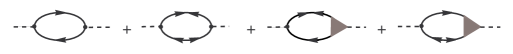
Figure 1: Graphs for the polarization tensor.

As can be seen, the field interaction with superfluid fermions should be described with the aid of four effective three-point vertices. There are two usual effective vertices (shown by dots) corresponding to the creation of a particle and a hole by the Z-field. Let us denote them as $\hat{\tau}\left(\mathbf{n;}\omega,\mathbf{k}\right)$ and $\hat{\tau}^{-}\left(\mathbf{n;}\omega,\mathbf{k}\right)\equiv\hat{\tau}^{T}\left(-\mathbf{n;}\omega,\mathbf{k}\right)$, respectively. We omit the Dirac indices in these symbolic notations. In reality, according to Eqs. (2) and (3), the non-relativistic ordinary vector vertex is represented by its temporal component, i.e. it is a scalar matrix in spin space. The ordinary axial-vector vertices of a particle and a hole are represented by space-vectors which components consist of spin matrices.

Two more vertices, represented by triangles, correspond to the creation of two particles or two holes. These so-called ”anomalous” vertices appear because the pairing interaction among quasi-particles is to be incorporated in the coupling vertex up to the same degree of approximation as in the self-energy of a quasiparticle Bogoliubov ; Nambu . This means that the anomalous effective vertices are given by infinite sums of diagrams with allowance for pair interaction in the ladder approximation, in the same way as in the gap equations.

Given by the sum of ladder-type diagrams Larkin , the anomalous vertices are to satisfy the Dyson’s equations symbolically depicted by graphs in Fig. 2a.

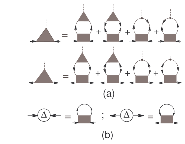
Figure 2: Dyson’s equations for the anomalous vertices (a), and the gap equations (b). Shaded rectangles represent the pairing interaction;

In these graphs, the rectangles denote pairing interaction, which in the channel of two quasiparticles is given by Eq. (5). The vertex equations are to be supplemented by the gap equation shown graphically in Fig. 2b. This equation, whose solution is assumed known, serves to eliminate the amplitude of the pair interaction from the vertex equations near the Fermi surface. The standard gap equation involves integrations over the regions far from the Fermi surface. This integration can be eliminated by means of the renormalization of the pairing interaction, as suggested in Ref. Leggett . Details of this calculation can be found in Leinson2012 .

The analytic form of the quasiparticle propagators in the momentum representation can be written as

$$\hat{G}=G\left(\varepsilon_{s},\mathbf{p}\right)\hat{1},~{}\ \ \hat{F}^{\left(1\right)}=F\left(\varepsilon_{s},\mathbf{p}\right)\left(\mathbf{\bar{b}\hat{\sigma}}\right)i\hat{\sigma}_{2},$$ (14)

$$\hat{F}^{\left(2\right)}=\hat{F}^{\left(1\right)\dagger}\left(-\varepsilon_{s},-\mathbf{p}\right)=i\hat{\sigma}_{2}\left(\mathbf{\bar{b}\hat{\sigma}}\right)F\left(-\varepsilon_{s},-\mathbf{p}\right).$$ (15)

Making use of the Matsubara calculation technique we define the scalar part of the Green functions

$$G\left(\varepsilon_{s},\mathbf{p}\right)=\frac{-i\varepsilon_{s}-\xi_{p}}{\varepsilon_{s}^{2}+E_{\mathbf{p}}^{2}},~{}\ \ F\left(\varepsilon_{s},\mathbf{p}\right)=\frac{\Delta}{\varepsilon_{s}^{2}+E_{\mathbf{p}}^{2}}.$$ (16)

Here $\varepsilon_{s}=\left(2s+1\right)\pi T$ with $s=0,\pm 1,\pm 2,...$ be the fermionic Matsubara frequency which depends on the temperature $T$, and

$$E=\sqrt{\xi^{2}+\Delta_{\mathbf{n}}^{2}}~{}$$ (17)

stands for the Bogolon energy. The angle-dependent energy gap is given by $\Delta_{\mathbf{n}}^{2}\equiv\Delta^{2}\bar{b}^{2}\left(\mathbf{n}\right)$.

It should be noted that, by virtue of Eq. (7), the amplitude $\Delta\left(T\right)$ is chosen as to represent the energy gap averaged over the Fermi surface. Thus determined, the energy gap gives a general measure of the pairing correction to the energy of the ground state in the preferred state.

In general, the ordinary vertices in the Dyson equations should be dressed owing to residual Fermi-liquid interactions. We neglect this effect, and account for the residual interactions by means of the effective nucleon mass only. In this case the ordinary vertices are as defined in Eqs. (2), (3). Namely, the non-relativistic ordinary vector vertex is represented by its temporal component

$$\hat{\tau}_{V}=\hat{\tau}_{V}^{-}=\hat{1}.$$ (18)

The ordinary axial-vector vertices of a particle and a hole are to be taken as

$$\hat{\tau}_{A}=\mathbf{\hat{\sigma},~{}}\hat{\tau}_{A}^{-}=\mathbf{\hat{\sigma}}^{T},$$ (19)

where the upperscript ”$T$” transposes the matrix.

In the case of pairing in the channel with spin, orbital and total angular momenta, $S=1,L=1,J=2$, respectively, one can search for the anomalous vertices near the Fermi surface in the form of expansions over the eigenfunctions of the total angular momentum $(J,M)$ with $J=2$ and $M=0,\pm 1,\pm 2$. For our calculations it is convenient to use vector notation which involves a set of mutually orthogonal complex vectors $\mathbf{b}_{M}\left(\mathbf{n}\right)$ in spin space which generate standard spin-angle matrices according to

$$\frac{1}{\sqrt{8\pi}}\mathbf{b}_{M}(\mathbf{n})\mathbf{\hat{\sigma}}i\hat{\sigma}_{2}\equiv\sum_{M_{S}+M_{L}=M}\left(\frac{1}{2}\frac{1}{2}\alpha\beta|1M_{S}\right)\left(11M_{S}M_{L}|2M\right)Y_{1,M_{L}}\left(\mathbf{n}\right),$$ (20)

where $\alpha,\beta=\uparrow,\downarrow$ denote spin projections.

These vectors are of the form

$$\mathbf{b}_{0} =\sqrt{1/2}\left(-n_{1},-n_{2},2n_{3}\right),\mathbf{b}_{1}=-\sqrt{3/4}\left(n_{3},in_{3},n_{1}+in_{2}\right),$$

$$\mathbf{b}_{2} =\sqrt{3/4}\left(n_{1}+in_{2},in_{1}-n_{2},0\right),\mathbf{b}_{-M}=\left(-\right)^{M}\mathbf{b}_{M}^{\ast}.$$ (21)

These are normalized by the condition

$$\left\langle\mathbf{b}_{M^{\prime}}^{\ast}\mathbf{b}_{M}\right\rangle=\delta_{M^{\prime}M}.$$ (22)

Generally speaking, the anomalous vertices are functions of the transferred energy and momentum $(\omega,\mathbf{k})$ and the direction $\mathbf{n}$ of the quasiparticle momentum. As was mentioned in Introduction, it is sufficient to evaluate the medium response function in the limit $\mathbf{k}\rightarrow 0$. Then the non-relativistic anomalous vector vertex can be expanded in the eigenfunctions of the total angular momentum $J=2$ in the form

$$\mathcal{\hat{T}}^{\left(1\right)}=\sum_{M}\mathcal{B}_{M}^{\left(1\right)}\left(\omega\right)\mathbf{b}_{M}\mathbf{\hat{\sigma}}i\hat{\sigma}_{2},$$ (23)

$$\mathcal{\hat{T}}^{\left(2\right)}=\sum_{M}\mathcal{B}_{M}^{\left(2\right)}\left(\omega\right)i\hat{\sigma}_{2}\mathbf{\hat{\sigma}b}_{M}.$$ (24)

Accordingly, the anomalous axial-vector vertices can be represented in the form

$$\mathbf{\hat{T}}^{\left(1\right)}=\sum_{M}\mathbf{B}_{M}^{\left(1\right)}\left(\omega\right)\mathbf{b}_{M}\mathbf{\hat{\sigma}}i\hat{\sigma}_{2},$$ (25)

$$\mathbf{\hat{T}}^{\left(2\right)}=\sum_{M}\mathbf{B}_{M}^{\left(2\right)}\left(\omega\right)i\hat{\sigma}_{2}\mathbf{\hat{\sigma}b}_{M}.$$ (26)

Making use of these general forms in the Dyson equations together with the corresponding ordinary vertices, after tedious computations, one can get Leinson2012 in the vector channel

$$\mathcal{B}_{M}^{\left(1\right)}=-\mathcal{B}_{M}^{\left(2\right)}\equiv\mathcal{B}_{M},$$ (27)

where $\mathcal{B}_{M}$ obeys the equation

$$\sum_{M^{\prime}}2\left\langle\left[\left(\Omega^{2}-\bar{b}^{2}\right)\mathbf{b}_{M}^{\ast}\mathbf{b}_{M^{\prime}}+\left(\mathbf{b}_{M}^{\ast}\mathbf{\bar{b}}\right)\left(\mathbf{b}_{M^{\prime}}\mathbf{\bar{b}}\right)\right]\mathcal{I}_{0}\right\rangle\mathcal{B}_{M^{\prime}}$$

$$+\left\langle\left(b_{M}^{2}-\bar{b}^{2}\right)A\right\rangle\mathcal{B}_{M}=2\Omega\left\langle\left(\mathbf{b}_{M}^{\ast}\mathbf{\bar{b}}\right)\mathcal{I}_{0}\right\rangle,$$ (28)

In the axial-vector channel one finds

$$\mathbf{B}_{M}^{\left(1\right)}=\mathbf{B}_{M}^{\left(2\right)}\equiv\mathbf{B}_{M}$$ (29)

with $\mathbf{B}_{M}$ satisfying the equation

$$\sum_{M^{\prime}}~{}2\left\langle\left[\Omega^{2}\mathbf{b}_{M}^{\ast}\mathbf{b}_{M^{\prime}}-\left(\mathbf{b}_{M}^{\ast}\mathbf{\bar{b}}\right)\left(\mathbf{b}_{M^{\prime}}\mathbf{\bar{b}}\right)\right]\mathcal{I}_{0}\right\rangle\mathbf{B}_{M^{\prime}}$$

$$+\left\langle\left(b_{M}^{2}-\bar{b}^{2}\right)A\right\rangle\mathbf{B}_{M}=-2i\Omega\left\langle\left(\mathbf{b}_{M}^{\ast}\mathbf{\times\bar{b}}\right)\mathcal{I}_{0}\right\rangle,$$ (30)

In the above expressions, the following notation is used:

$$\Omega=\frac{\omega}{2\Delta},$$ (31)

the functions $\mathcal{I}_{0}\left(\omega,\mathbf{n},T\right)$ and $A\left(\mathbf{n},T\right)$ are given by

$$\mathcal{I}_{0}\left(\omega\mathbf{,n}\right)=\int_{-\infty}^{\infty}\frac{d\xi}{E}\frac{\Delta^{2}}{4E^{2}-\left(\omega+i0\right)^{2}}\tanh\frac{E}{2T}~{},$$ (32)

$$A\left(\mathbf{n}\right)\equiv\int_{-\infty}^{\infty}d\xi\left(\frac{1}{2E}\tanh\frac{E}{2T}-\frac{1}{2\xi}\tanh\frac{\xi}{2T}\right).$$ (33)

From Eqs. (28) and (30) it is seen that an accurate calculation of the anisotropic anomalous vertices at arbitrary temperatures apparently requires numerical computations. It would be desirable, however, to get reasonable analytic expressions for the anomalous vertices, which can be applied to a calculation of the neutrino energy losses. To proceed, let us notice that the anisotropy of the functions $\mathcal{I}_{0}\left(\omega\mathbf{,n}\right)$ and $A\left(\mathbf{n}\right)$ is due to the dependence of the energy of the Bogolons (17) on the direction of the momentum relative to the quantization axis. In a uniform system without external fields and at absolute zero, the orientation of the quantization axis is arbitrary. For equilibrium at a non-zero temperature this leads to the formation of a loose domain structure br60 , where each microscopic domain has a randomly oriented preferred axis. This fact is normally used in order to simplify the calculations by replacing the angle-dependent energy gap with some effective isotropic value (see, e.g. bhy01 ; gh05 ).

Making use of this trick we replace the angle-dependent energy gap $\Delta_{\mathbf{n}}^{2}\equiv\Delta^{2}\bar{b}^{2}\left(\mathbf{n}\right)$ in the Bogolons energy by its average value $\left\langle\Delta^{2}\bar{b}^{2}\left(\mathbf{n}\right)\right\rangle=\Delta^{2}$, in accordance with Eq. (7). Then the functions $\mathcal{I}_{0}$ and $A$ can be moved out the integrals over the solid angle in Eqs. (28) and (30). Using further the axial symmetry of the order parameter, Eq. (22) and the fact that

$$\left\langle\left(\mathbf{b}_{M}^{\ast}\mathbf{b}_{M}-\bar{b}^{2}\right)\right\rangle=0~{}$$ (34)

we get for the vector channel the equation

$$\left(\Omega^{2}-\left\langle\bar{b}^{2}\mathbf{b}_{M}^{\ast}\mathbf{b}_{M}\right\rangle\right)\mathcal{B}_{M}+\sum_{M^{\prime}}\left\langle\left(\mathbf{b}_{M}^{\ast}\mathbf{\bar{b}}\right)\left(\mathbf{b}_{M^{\prime}}\mathbf{\bar{b}}\right)\right\rangle\mathcal{B}_{M^{\prime}}=\Omega\left\langle\mathbf{b}_{M}^{\ast}\mathbf{\bar{b}}\right\rangle.$$ (35)

In the axial channel we obtain the equation

$$\Omega^{2}\mathbf{B}_{M}-\sum_{M^{\prime}}\left\langle\left(\mathbf{b}_{M}^{\ast}\mathbf{\bar{b}}\right)\left(\mathbf{b}_{M^{\prime}}\mathbf{\bar{b}}\right)\right\rangle\mathbf{B}_{M^{\prime}}=-i\Omega\left\langle\left(\mathbf{b}_{M}^{\ast}\mathbf{\times\bar{b}}\right)\right\rangle.$$ (36)

The specific form of solutions to Eqs. (35) and (36) depends on the phase state of the condensate.

An inspection of Eqs (9) and (21) allows one to conclude that for the ground state with $M_{J}=0$

$$\mathbf{\bar{b}}_{M=0}\mathbf{=b}_{0}.$$ (37)

In this case we get $\left\langle\mathbf{b}_{M}^{\ast}\mathbf{\bar{b}}\right\rangle=\delta_{M,0}$, and the only non-vanishing values of $\left\langle\mathbf{b}_{M}^{\ast}\mathbf{\times\bar{b}}\right\rangle$ correspond to $M=\pm 1$. Simple calculations give

$$\mathcal{B}_{M}=\frac{2\Delta}{\omega}\delta_{M,0}$$ (38)

and

$$~{}\mathbf{B}_{1}=\sqrt{\frac{3}{2}}\frac{\Delta\omega}{\omega^{2}-\Delta^{2}/5}\mathbf{e}^{\ast},~{}\mathbf{B}_{-1}=\sqrt{\frac{3}{2}}\frac{\Delta\omega}{\omega^{2}-\Delta^{2}/5}\mathbf{e}$$ (39)

where

$$\mathbf{e}=\left(1,i,0\right).$$ (40)

Substituting the obtained expressions to Eqs. (23) - (26) we get the anomalous vertices which, together with the ordinary vertices (18) and (19), can be used to calculate the weak polarization tensor of the medium. We now turn to a calculation of the corresponding correlation functions separately in the vector and axial channel of weak interactions.

V Correlation functions of weak currents

V.1 Vector channel

Following to the graphs of Fig. 1 the vector-vector part of the polarization tensor, $\Pi_{\mu\nu}^{V}=\delta_{\mu 0}\delta_{\nu 0}\Pi_{00}^{V}$, is given by analytic continuation of the following Matsubara sums to the upper half-plane of the complex variable $\omega$:

$$\Pi_{00}^{V}\left(\omega\right)=T\sum_{\mathbf{p,}\varepsilon_{s}}\mathrm{Tr}\left(\hat{G}_{+}\hat{G}+\hat{F}_{+}^{\left(1\right)}\hat{F}^{\left(2\right)}+\hat{F}_{+}^{\left(1\right)}\mathcal{\hat{T}}^{\left(1\right)}\hat{G}+\hat{G}_{+}\mathcal{\hat{T}}^{\left(2\right)}\hat{F}^{\left(2\right)}\right).$$ (41)

We use the notations $\hat{G}_{+}=\hat{G}\left(\varepsilon_{s}+\omega_{n},\mathbf{p}\right)$, $\hat{F}_{+}^{\left(1\right)}=\hat{F}^{\left(1\right)}\left(\varepsilon_{s}+\omega_{n},\mathbf{p}\right)$, where $\omega_{n}=2i\pi Tn$ with $n=0,\pm 1,\pm 2...$ is a bosonic Matsubara frequency.

The two first terms in the right of Eq. (41) describe the medium polarization without anomalous contributions. The  long-wave limit of this ordinary contribution in the vector channel can be found in the form

$$\left(\Pi_{00}^{V}\right)_{\mathsf{ordin}}\simeq-4\frac{p_{F}m^{\ast}}{\pi^{2}}\left\langle\bar{b}^{2}\left(\mathbf{n}\right)\mathcal{I}_{0}\left(\mathbf{n,}\omega\right)\right\rangle$$

Evidently this expression does not satisfy the condition of current conservation $\omega\Pi_{00}^{V}=k_{i}\Pi_{i0}^{V}$, which in the long-wave limit $\mathbf{k}\rightarrow 0$ requires $\Pi_{00}^{V}\left(\omega>0\right)=0$.

The last two terms in Eq. (41), with the vertices indicated in Eqs. (23), (24), represent the anomalous contributions. According to Eqs. (27) and (38) the anomalous vector vertices can be written as

$$\mathcal{\hat{T}}^{\left(1\right)}=\frac{2\Delta}{\omega}\mathbf{\bar{b}\hat{\sigma}}i\hat{\sigma}_{2},$$

and

$$\mathcal{\hat{T}}^{\left(2\right)}=-\frac{2\Delta}{\omega}i\hat{\sigma}_{2}\mathbf{\hat{\sigma}\bar{b}}.$$

Straightforward calculations give in the long-wave limit

$$\left(\Pi_{00}^{V}\right)_{\mathsf{anom}}\simeq 4\frac{p_{F}m^{\ast}}{\pi^{2}}\left\langle\bar{b}^{2}\left(\mathbf{n}\right)\mathcal{I}_{0}\left(\mathbf{n,}\omega\right)\right\rangle.$$

We finally find

$$\Pi_{00}^{V}\left(\omega,\mathbf{0}\right)=\left(\Pi_{00}^{V}\right)_{\mathsf{ordin}}+\left(\Pi_{00}^{V}\right)_{\mathsf{anom}}=0,$$ (42)

as is required by the current conservation condition. This proves explicitly that the neutrino emissivity via the vector channel, as initially obtained in Yakovlev1999 , is a subject of inconsistency.

V.2 Axial channel

In the axial channel, the ordinary vertices (19) and anomalous vertices (45), (46) consist of only space components, and thus $\Pi_{\mu\nu}^{A}\simeq\delta_{\mu i}\delta_{\nu j}C_{A}^{2}\Pi_{ij}^{A}$, where $\Pi_{ij}^{A}$ is to be found as the analytic continuation of the following Matsubara sums:

$$\Pi_{ij}^{A}\left(\omega\right) = T\sum_{\mathbf{p,}\varepsilon_{s}}\mathrm{Tr}\left(\hat{\sigma}_{i}\hat{G}_{+}\hat{\sigma}_{j}\hat{G}+\hat{\sigma}_{i}\hat{F}_{+}^{\left(1\right)}\hat{\sigma}_{j}^{-}\hat{F}^{\left(2\right)}\right)$$ (43)

$$+T\sum_{\mathbf{p,}\varepsilon_{s}}\mathrm{Tr}\left(\hat{\sigma}_{i}\hat{F}_{+}^{\left(1\right)}\hat{T}_{j}^{\left(1\right)}\hat{G}+\hat{\sigma}_{i}\hat{G}_{+}\hat{T}_{j}^{\left(2\right)}\hat{F}^{\left(2\right)}\right).$$

Here the first line represents the ordinary contribution and the second line is the contribution of the anomalous interactions. The ordinary contribution can be evaluated in the form

$$\left(\Pi_{ij}^{A}\right)_{\mathsf{ordin}}=-4\frac{p_{F}m^{\ast}}{\pi^{2}}\left\langle\left(\bar{b}^{2}\left(\mathbf{n}\right)\delta_{ij}-\bar{b}_{i}\left(\mathbf{n}\right)\bar{b}_{j}\left(\mathbf{n}\right)\right)\mathcal{I}_{0}\left(\mathbf{n,}\omega\right)\right\rangle$$ (44)

In the case of $M_{J}=0$ when $\mathbf{\bar{b}=b}_{0}$, from Eqs. (25), (26) and (39), (40) we get

$$\mathbf{\hat{T}}^{\left(1\right)}=\sqrt{\frac{3}{2}}\frac{\omega\Delta}{\left(\omega+i0\right)^{2}-\Delta^{2}/5}\left[\mathbf{e}^{\ast}\left(\mathbf{\hat{\sigma}b}_{1}\right)i\hat{\sigma}_{2}+\mathbf{e}\left(\mathbf{\hat{\sigma}b}_{-1}\right)i\hat{\sigma}_{2}\right]~{},$$ (45)

$$\mathbf{\hat{T}}^{\left(2\right)}=\sqrt{\frac{3}{2}}\frac{\omega\Delta}{\left(\omega+i0\right)^{2}-\Delta^{2}/5}\left[i\hat{\sigma}_{2}\left(\mathbf{\hat{\sigma}b}_{1}\right)\mathbf{e}^{\ast}+i\hat{\sigma}_{2}\left(\mathbf{\hat{\sigma}b}_{-1}\right)\mathbf{e}\right].$$ (46)

Poles of the vertex function correspond to collective eigen modes of the system (see, e.g. Leinson2012 ; Leinson2010a ; Leinson2011 ). Thus, the pole at $\omega^{2}=\Delta^{2}/5$ signals the existence of collective oscillations of the total angular momentum. The pole location on the complex $\omega$-plain is chosen so as to obtain a retarded vertex.

Principally, the decay of these collective oscillations into neutrino pairs is also possible by giving the additive contribution into neutrino energy losses via the axial channel of weak interactions. Later we will return to this problem. Here we concentrate on the PBF processes. In this case we are interested in $\omega>2\Delta\bar{b}\left(\theta\right)\geq\sqrt{2}\Delta$, and a small term $\Delta^{2}/5\ll$ $\omega^{2}$ in the denominator of Eqs. (45) and (46) can be discarded to obtain simpler expressions

$$\mathbf{\hat{T}}^{\left(1\right)}\left(\mathbf{n}\right)=\sqrt{\frac{3}{2}}\frac{\Delta}{\omega}\left[\mathbf{e}^{\ast}\left(\mathbf{\hat{\sigma}b}_{1}\right)i\hat{\sigma}_{2}+\mathbf{e}\left(\mathbf{\hat{\sigma}b}_{-1}\right)i\hat{\sigma}_{2}\right]~{},$$ (47)

$$\mathbf{\hat{T}}^{\left(2\right)}\left(\mathbf{n}\right)=\sqrt{\frac{3}{2}}\frac{\Delta}{\omega}\left[i\hat{\sigma}_{2}\left(\mathbf{\hat{\sigma}b}_{1}\right)\mathbf{e}^{\ast}+i\hat{\sigma}_{2}\left(\mathbf{\hat{\sigma}b}_{-1}\right)\mathbf{e}\right].$$ (48)

Substituting expressions (47) and (48) in the second line of Eq. (43) we obtain the anomalous part of the axial polarization tensor in the long-wave limit

$$\left(\Pi_{ij}^{A}\right)_{\mathsf{anom}}=3\frac{p_{F}m^{\ast}}{\pi^{2}}\left\langle\left(\delta_{ij}-\delta_{i3}\delta_{j3}\right)\bar{b}^{2}\left(\mathbf{n}\right)\mathcal{I}_{0}\left(\mathbf{n,}\omega\right)\right\rangle.$$ (49)

Summing together the contributions, given in Eqs. (44) and (49), we obtain the complete response function in the axial channel:

$$\Pi_{ij}^{A}\left(M_{J}=0\right) =-4\frac{p_{F}m^{\ast}}{\pi^{2}}\left\langle\left[\bar{b}^{2}\delta_{ij}-\bar{b}_{i}\bar{b}_{j}\right]\mathcal{I}_{0}\right\rangle$$

$$+3\frac{p_{F}m^{\ast}}{\pi^{2}}\left\langle\left(\delta_{ij}-\delta_{i3}\delta_{j3}\right)\bar{b}^{2}\mathcal{I}_{0}\right\rangle.$$ (50)

The imaginary part of the function $\mathcal{I}_{0}\left(\mathbf{n,}\omega\right)$ arises from the poles of the integrand in Eq. (32) at $\omega=\pm 2E$:

$$\bar{b}^{2}\left(\mathbf{n}\right)\mathrm{Im}\mathcal{I}_{0}\left(\mathbf{n,}\omega\right)=\Theta\left(\omega-2\Delta_{\mathbf{n}}\right)\frac{\pi\Delta_{\mathbf{n}}^{2}}{2\omega\sqrt{\omega^{2}-4\Delta_{\mathbf{n}}^{2}}}\tanh\frac{\omega}{4T}.$$ (51)

Using Eq. (51) and Eqs. (13), (42), and (50) we obtain the imaginary part of the weak polarization tensor for the ³P${}_{2}\left(M_{J}=0\right)$ superfluid neutron liquid

$$\mathrm{Im}\Pi_{\mu\nu}\left(\omega>0\right)=-\delta_{\mu i}\delta_{\nu j}C_{A}^{2}p_{F}m^{\ast}\frac{2}{\pi}\frac{1}{\omega}\tanh\frac{\omega}{4T}$$

$$\times\int\frac{d\mathbf{n}}{4\pi}\left[\delta_{ij}-\frac{\bar{b}_{i}\bar{b}_{j}}{\bar{b}^{2}}-\frac{3}{4}\left(\delta_{ij}-\delta_{i3}\delta_{j3}\right)\right]\frac{\Delta_{\mathbf{n}}^{2}\Theta\left(\omega-2\Delta_{\mathbf{n}}\right)}{\sqrt{\omega^{2}-4\Delta_{\mathbf{n}}^{2}}}.$$ (52)

VI PBF neutrino energy losses

Now we substitute the obtained weak polarization tensor to Eq. (12) for the neutrino emissivity. Contraction of the tensor (52) with $\left(K^{\mu}K^{\nu}-K^{2}g^{\mu\nu}\right)$ gives:

$$\mathrm{Im}\Pi_{\mu\nu}\left(\omega\right)\left(K^{\mu}K^{\nu}-K^{2}g^{\mu\nu}\right)=-C_{A}^{2}\frac{p_{F}m^{\ast}}{\pi}\frac{1}{\omega}\tanh\frac{\omega}{4T}$$

$$\times\int\frac{d\mathbf{n}}{4\pi}\left[2\left(\omega^{2}-k_{\parallel}^{2}\right)-k_{\perp}^{2}\right]\frac{\Delta_{\mathbf{n}}^{2}\Theta\left(\omega-2\Delta_{\mathbf{n}}\right)}{\sqrt{\omega^{2}-4\Delta_{\mathbf{n}}^{2}}},$$ (53)

where we denote

$$k_{\parallel}^{2}=\frac{1}{\bar{b}^{2}}\left(\mathbf{k\bar{b}}\right)^{2}~{},~{}k_{\perp}^{2}=k^{2}-k_{\parallel}^{2}.$$ (54)

After some algebra we find the neutrino emissivity in the form:

$$Q\simeq\frac{2}{15\pi^{5}}G_{F}^{2}C_{A}^{2}\mathcal{N}_{\nu}p_{F}m^{\ast}T^{7}\int\frac{d\mathbf{n}}{4\pi}\frac{\Delta_{\mathbf{n}}^{2}}{T^{2}}\int_{0}^{\infty}dx\frac{z^{4}}{\left(1+\exp z\right)^{2}}~{},$$ (55)

where $\Delta_{\mathbf{n}}^{2}\equiv\Delta^{2}\,\bar{b}^{2}\left(\mathbf{n}\right)=\frac{1}{2}\Delta^{2}\left(1+3\cos^{2}\theta\right)$, and $z=\sqrt{x^{2}+\Delta_{\mathbf{n}}^{2}/T^{2}}$.

It is necessary to notice that a definition of the gap amplitude is ambiguous in the literature. For example, in the case of $M_{J}=0$, our gap amplitude is $\sqrt{2}$ times larger than the gap amplitude in Ref. Yakovlev1999 (denote it $\Delta_{\text{{YKL}}}$), where it is defined by the relation $\Delta_{\mathbf{n}}^{2}=\Delta_{\text{{YKL}}}^{2}\left(1+3\cos^{2}\theta\right)$. However, the total anisotropic gap $\Delta_{\mathbf{n}}$ entering the energy of the quasiparticles is the same in both calculations, since $\Delta/\sqrt{2}=\Delta_{\text{{YKL}}}$.

Returning to the standard physical units we get Leinson2010

$$Q = \frac{4G_{F}^{2}p_{F}m^{\ast}}{15\pi^{5}\hbar^{10}c^{6}}\left(k_{B}T\right)^{7}\mathcal{N}_{\nu}R$$ (56)

$$= 1.170\,\times 10^{21}\frac{m^{\ast}}{m}\frac{p_{F}}{mc}T_{9}^{7}\mathcal{N}_{\nu}R~{}\ \frac{\mathsf{erg}}{\mathsf{cm}^{3}\mathsf{s}}~{}.$$

Remind that $G_{F}$ is the Fermi coupling constant, $C_{A}\simeq 1.26$ is the axial-vector weak coupling constant of a neutron, and $\mathcal{N}_{\nu}=3$ is the number of neutrino flavors; $p_{F}$ is the Fermi momentum of neutrons, $m^{\ast}\equiv p_{F}/v_{F}$ is the effective neutron mass; $m$ is bare nucleon mass, $T_{9}=T/(10^{9}\mathsf{K})$, $k_{B}$ is the Boltzmann constant, and

$$R=\frac{1}{2}C_{A}^{2}F_{t}.$$ (57)

The function $F_{t}$ is given by

$$F_{t}=\int\frac{d\mathbf{n}}{4\pi}y^{2}\int_{0}^{\infty}dx\frac{z^{4}}{\left(1+\exp z\right)^{2}}.$$ (58)

Here the notation is used$\ z=\sqrt{x^{2}+y^{2}}$ with $y=\Delta_{\mathbf{n}}/T$. The unit vector $\mathbf{n=p}/p$ defines the polar angles $\left(\theta,\varphi\right)$ on the Fermi surface.

It is necessary to stress that Eq.(55) as well as Eq. (56) involves the anomalous contributions into both the channels of weak interactions (vector and axial). A comparison of the formula (57) with Eq. (28) of the work Yakovlev1999 , where the PBF neutrino losses were obtained ignoring the anomalous interactions, allows one to see that the anomalous contributions not only completely suppress the vector channel of weak interactions, but also suppress four times the energy losses through the axial channel. The resulting reduction of the emissivity of the PBF processes in neutron matter is Leinson2010 :

$$\frac{C_{A}^{2}}{2\left(C_{V}^{2}+2C_{A}^{2}\right)}\simeq 0.19.$$ (59)

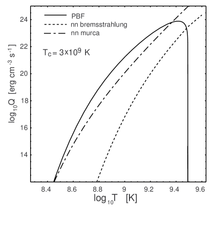
Figure 3: PBF neutrino emissivity versus temperature $T$ in comparison with the modified Urca and bremsstrahlung emissivities at $k_{F}=1.7$.

In spite of the so strong reduction, the neutrino emissivity caused by the PBF processes can be the most powerful mechanism of the energy losses from the NS core below the critical temperature $T_{c}$. In Fig. 3, the PBF neutrino emissivity, as given in Eq. (55), is shown together with the emissivities of modified Urca processes and bremsstrahlung multiplied by the corresponding suppression factors resulting from superfluidity, as obtained in Ref. YKGH .

The emissivity from the PBF dominates everywhere below the critical temperature for the ³P₂ superfluidity except the narrow temperature domain near the critical point, where the modified Urca processes are more operative.

VII Decay of the eigenmodes of the condensate

We now turn to an estimate of the neutrino energy losses due to decay of thermally excited oscillations of the spin-triplet condensate of neutrons. These eigenmodes represent collective oscillations of the direction of total angular momenta of Cooper pairs which generate fluctuations of axial currents in the superfluid system (spin density fluctuations). The energy of the collective mode excitation $\omega=\Delta/\sqrt{5}$ is smaller than the energy gap in the quasiparticle spectrum. In this case the function $\mathcal{I}_{0}\left(\mathbf{n,}\omega\right)$, given in Eq. (32), is real, and the imaginary part of the axial polarization tensor (43) arises from the pole part of the functions $\mathbf{\hat{T}}^{\left(1,2\right)}$ at $\omega^{2}-\Delta^{2}/5=0$.

With the aid of Sokhotsky’s formula, $\left(\chi+i0\right)^{-1}=\mathcal{P}\left(1/\chi\right)-i\pi\delta\left(\chi\right)$, from the second line of Eq. (43) we get

$$\mathrm{Im}\Pi_{\mu\nu}\left(\omega>0\right) =-\delta_{\mu i}\delta_{\nu j}\left(\delta_{ij}-\delta_{i3}\delta_{j3}\right)$$

$$\times\frac{3}{2\pi}C_{A}^{2}p_{F}m^{\ast}\left\langle\bar{b}^{2}\mathcal{I}_{0}\right\rangle\omega\delta\left(\omega-\Delta/\sqrt{5}\right).$$ (60)

The neutrino luminosity per unit volume is proportional to the product of the total phase volume available to the outgoing neutrinos and the total energy of the neutrino pair. This explains the temperature dependence of the PBF neutrino emissivity, as given in Eq. (55). The presence of the delta-function $\delta\left(\omega-\Delta/\sqrt{5}\right)$ in Eqs. (60) restricts the total energy of the neutrino pair by the dispersion relation and thus substantially reduces the total volume available to neutrino pairs in the phase space. Integration over the phase volume will result to appearance of the factor $\left(\Delta/\sqrt{5}\right)^{7}$ instead of $T^{7}$. Just below the superfluid transition temperature, where the main splash of the PBF neutrino emission occurs, the collective mode energy $\omega_{s}=\Delta\left(T\right)/\sqrt{5}$ is small as compared to the temperature. As a result the emissivity due to the collective mode decays is many orders of magnitude slower than the PBF emissivity.

One might expect the two emissivities become comparable at sufficiently low temperature $T\lesssim\Delta\left(T\right)/\sqrt{5}$. It is necessary to notice, however, that our estimate is valid only when the anisotropic energy gap is replaced by its average value in the anomalous vertices. Such an approximation is good for the PBF processes but not for the eigen modes. The exact account of the anisotropy dramatically reduces the neutrino losses due to the collective mode decays Leinson2013 .

VIII Application to cooling modeling of neutron stars

The strong suppression of the vector PBF channel is basically incorporated in the cooling simulations codes (e.g., Gupta2007 ; Page2009 ; Shternin2015 ; Potekhin2015 ; Han2017 ). In the case of ¹S₀ pairing of neutrons the suppression of the vector channel should be important in the cooling interpretation of a NS crust as the cooling time-scale of the crust is sensitive to the rates of neutrino emission. Quenching of the neutrino emission, found in the case of ${}^{1}S_{0}$ pairing, leads to higher temperatures that can be reached in the crust of an accreting NS. This allows one to explain the observed data of superbursts triggering Cumming2006 ; Gupta2007 ; Keek2008 ; Brown2009 , which was in dramatic discrepancy with the previous theory of the crust cooling. However, the suppression of the neutron ¹S₀ PBF process does not lead to a distinguishable effect in the long-term cooling ($>$ 1000 years) of the star Page2009 .

The neutron pairing in the NS core, is expected to occurs into the spin-triplet ³P₂ state (a small ³F₂ admixture caused by tensor forces is normally neglected). Just a few years ago, suppression of the PBF neutrino emission due to spin-triplet neutron pairing in the NS core was included in the neutron star cooling codes only by complete suppression of the vector channel, while the emission in the axial vector channel remained unchanged Page2009 ; Page2011 . This corresponds to the reduction factor of $0.76$ with respect to the PBF emissivity previously obtained in Yakovlev1999 , which led the authors to the conclusion that, within the minimal cooling paradigm, the closing of the vector channel of the PBF neutrino emission does not significantly affect the long-term cooling of NSs. The reason is that the long-term cooling is controlled by the axial channel of the PBF emissivities.

The suppression factor for PBF neutrino radiation given in Eq. (59) involves two physical phenomena: (i) total suppression of the vector channel, and (ii) the fourfold suppression of the axial channel caused by the anomalous weak interactions. For the first time the suppression of the axial PBF channel was implemented in a simulation of the Cas A NS cooling in Shternin2011 ; Elshamouty2013 . It was found that the whole set of observations is quite consistent with the theoretical suppression factor of $0.19$. This factor, presented in Eq. (59), is now commonly used for suppression of the PBF reactions in spin-triplet superfluid neutron matter of the NS cores (e.g. Shternin2015 ; Potekhin2015 ; Beloin2018 ; Fortin2018 ).

An exhaustive numerical analysis of the anomalous axial PBF contribution to the temporal evolution of the NS cooling is presented in Potekhin2018 . The interested reader can get a clear idea about importance of this contribution from Figs. 2 and 3 of that work, where the authors present the NS cooling curves for the cases with and without the anomalous contribution.

IX Conclusion

We have discussed the important role of anomalous weak interactions in mechanisms of neutrino emission taking place in fermionic superfluids typical for the NS cores. It is established that due to the anomalous contributions the PBF neutrino emissivity from the vector channel is almost completely suppressed and can be ignored. This result is in agreement with the conservation of vector current in weak interactions. In the case of spin-singlet pairing the neutrino emission through the axial-vector channel is also suppressed because the total spin of the Cooper pair $S=0$ is conserved in the non-relativistic case. Thus the neutrino energy losses due to singlet-state pairing of baryons can, in practice, be ignored in simulations of NS cooling. This makes unimportant the PBF neutrino losses from pairing of protons or hyperons.

The minimal cooling paradigm assummes that the direct Urca processes and any exotic fast reactions are not operative in the NC core. In this scenario, neutrino emission at the long-term cooling epoch comes mainly from modified Urca processes, nn-bremsstrahlung, and from the ”PBF” processes, which arise in the presence of spin-triplet superfluidity of neutrons Page2009 . We have shown that the anomalous weak interactions in the ³P₂ superfluid suppress the PBF neutrino emission, although not so sharply as in spin-singlet superfluid liquids. Namely, the vector channel of weak interactions is again strongly suppressed and can be ignored while the neutrino losses through the axial channel are suppressed only partially. Despite of the approximately fivefold total suppression, the PBF mechanism of the neutrino energy losses is still operative. In many cases, especially for temperatures near the critical superfluidity temperature of neutrons, the PBF neutrino reactions can dominate and should be accurately taken into account.

References

- (1) Friman, B. L., & Maxwell, O. V., ”Neutrino emissivities of neutron stars”, ApJ 232, 541, 1979
- (2) Tsuruta, S., ”Neutron stars - Current cooling theories and observational results”, Comments Astrophys. 11, 151, 1986
- (3) Flowers E., Ruderman M., Sutherland P., ”Neutrino pair emission from finite-temperature neutron superfluid and the cooling of young neutron stars”, Astrophys. J., 205, 541, 1976
- (4) Voskresensky D., Senatorov A., ”Emission of Neutrinos by Neutron Stars”, Sov. Phys. JETP 63, 885, 1986
- (5) Voskresensky D., Senatorov A., ”Description of Nuclear Interaction in Keldysh’s Diagram Technique and Neutrino Luminosity of Neutron Stars”, Sov. J. Nucl. Phys. 45, 411, 1987
- (6) Yakovlev D., Kaminker A., Levenfish K., ”Neutrino emission due to Cooper pairing of nucleons in cooling neutron stars”, A&A, 343, 650, 1999
- (7) Schaab Ch., Voskresensky D., Sedrakian A.D.,Weber F.,Weigel M.K., ”Impact of medium effects on the cooling of non-superfluid and superfluid neutron stars, A&A 321, 591, 1997
- (8) Balberg S., Barnea N., ”S-wave pairing of hyperons in dense matter”, Phys. Rev. C, 57, 409, 1998
- (9) Ch. Schaab, S. Balberg, J. Schaffner-Bielich, ”Implications of Hyperon Pairing for Cooling of Neutron Stars”, ApJL, 504, L99, 1998
- (10) Page D., In: Many Faces of Neutron Stars (eds. R. Buccheri, J. van Peredijs, M. A. Alpar. Kluver, Dordrecht, 1998) p. 538.
- (11) Yakovlev D. G., Kaminker A. D., Levenfish K. P., In: Neutron Stars and Pulsars (ed. N. Shibazaki et al., Universal Akademy Press, Tokio, 1998) p. 195.
- (12) Page D., Lattimer J. M., Prakash M., Steiner A. W., ”Minimal Cooling of Neutron Stars: A New Paradigm”, Astrophys. J. Supp. 155, 623, 2004
- (13) Leinson L., Pérez A., ”Vector current conservation and neutrino emission from singlet-paired baryons in neutron stars”, Phys. Lett. B 638, 114, 2006
- (14) Leinson L., ”BCS approximation to the effective vector vertex of superfluid fermions”, Phys. Rev. C, 78, 015502, 2008
- (15) Kolomeitsev E. E., Voskresensky D. N., ”Neutrino emission due to Cooper-pair recombination in neutron stars reexamined”, Phys. Rev. C, 77, 065808, 2008
- (16) Steiner A. W. and Reddy S, ”Superfluid response and the neutrino emissivity of neutron matter”, Phys. Rev. C 79, 015802, 2009
- (17) Sedrakian A., Müther H., and Schuck P., ”Vertex renormalization of weak interactions and Cooper-pair breaking in cooling compact stars”, Phys. Rev. C 76, 055805, 2007
- (18) Gupta S., Brown E. F., Schatz H., Moller P., and Kratz K.-L., ”Heating in the Accreted Neutron Star Ocean: Implications for Superburst Ignition”, Astrophys. J. 662, 1188, 2007
- (19) Cumming A., Macbeth J., Zand J. J. M. I. & Page D., ”Long Type I X-Ray Bursts and Neutron Star Interior Physics”, Astrophys. J., 646, 429, 2006
- (20) Lattimer, J. M., van Riper, K. A., Prakash, M., & Prakash, M., ”Rapid cooling and the structure of neutron stars”, ApJ 425, 802, 1994
- (21) Page, D. 2009, in Neutron Stars and Pulsars, Ed. W. Becker, Springer Verlag, Astrophysics & Space Science Library, p. 247-288.
- (22) Page D., Lattimer J., Prakash M., Steiner A., ”Neutrino Emission from Cooper Pairs and Minimal Cooling of Neutron Stars”, Astrophys. J., 707, 1131, 2009
- (23) Tamagaki R., ”Superfluid state in neutron star matter. I. Generalized Bogoliubov transformation and existence of 3P2 gap at high density”, Prog. Theor. Phys., 44, 905, 1970
- (24) Takatsuka, T., ”Energy Gap in Neutron-Star Matter”, Prog. Theor. Phys. 48, 1517, 1972
- (25) Ofengeim D. D., Kaminker A. D., Klochkov D., Suleimanov V., Yakovlev D. G., ”Analysing neutron star in HESS J1731-347 from thermal emission and cooling theory”, Mon.Not.Roy.Astron.Soc. 454, 2668, 2015
- (26) Ofengeim D. D., Fortin M., Haensel P., Yakovlev D. G. and Zdunik J. L., ”Neutrino luminosities and heat capacities of neutron stars in analytic form”, Phys.Rev. D 96, 043002, 2017
- (27) Leinson L. B., ”Neutrino emission from triplet pairing of neutrons in neutron stars”, Phys. Rev. C 81, 025501, 2010
- (28) Han S. and Steiner A. W., ”Cooling of neutron stars in soft x-ray transients”, Phys.Rev. C 96, 035802, 2017
- (29) Shternin P. S., Yakovlev D. G., ”Self-similarity relations for cooling superfluid neutron stars”, Mon.Not.Roy.Astron.Soc. 446, 3621, 2015
- (30) Potekhin A. Y., Pons J. A., Page D., ”Neutron Stars—Cooling and Transport”, Space Sci.Rev. 191, 239, 2015
- (31) Page D., Prakash M., Lattimer J.M. and Steiner A.W., ” Rapid Cooling of the Neutron Star in Cassiopeia A Triggered by Neutron Superfluidity in Dense Matter”, Phys. Rev. Lett. 106, 081101
- (32) Shternin P., Yakovlev D., Heinke C., Ho W., Patnaude D., ”Cooling neutron star in the Cassiopeia A supernova remnant: evidence for superfluidity in the core”, Mon.Not.Roy.Astron.Soc., 412, L108, 2011
- (33) Leinson L. B., ”Superfluid phases of triplet pairing and rapid cooling of the neutron star in Cassiopeia A”, Phys. Lett. B, 741, 87, 2015
- (34) Leinson L. B., ”Collective modes of the order parameter in a triplet superfluid neutron liquid”, Phys. Rev. C 85, 065502, 2012
- (35) Okun’ L. B., ”Leptons and Quarks”, World Scientific Publishing Co. Pte. Ltd., 2014
- (36) Bogoliubov N. N., ”A new method in the theory of superconductivity. I.”, Soviet Phys. 34, 41, 1958; Bogoliubov N. N., ”A new method in the theory of superconductivity. III.”, Soviet Phys. 34, 51, 1958
- (37) Nambu Y., ”Quasi-Particles and Gauge Invariance in the Theory of Superconductivity”, Phys. Rev. 117, 648, 1960
- (38) Larkin A. I. and Migdal A. B., ”Theory of superfluid Fermi liquid. Application to the nucleus”, Sov. Phys. JETP 17, 1146, 1963
- (39) Leggett A. J., ”Theory of a Superfluid Fermi Liquid. I. General Formalism and Static Properties”, Phys. Rev., 140, 1869, 1965; Leggett A. J., ”Theory of a Superfluid Fermi Liquid. II. Collective Oscillations”, Phys. Rev., 147, 119, 1966
- (40) Hoffberg M., Glassgold A., Richardson R., Ruderman M., ”Anisotropic Superfluidity in Neutron Star Matter”, Phys. Rev. Lett., 24, 775, 1970
- (41) Baldo M., Cugnon J., Lejeune A., Lombardo U., ”Proton and neutron superfluidity in neutron star matter”, Nucl. Phys.A, 536, 349, 1992
- (42) Elgarøy O. ., Engvik L., Hjorth-Jensen M., Osnes E., ”Triplet pairing of neutrons in 3P2-stable neutron star matter”, Nucl. Phys. A, 607, 425, 1996
- (43) J. B. Ketterson and S. N. Song, ”Superconductivity”, (University press, Cambridge, 1999), p. 414
- (44) Brueckner K. A., Soda T., Anderson P. W., Morel P., ”Level Structure of Nuclear Matter and Liquid He3”, Phys. Rev. 118, 1442, 1960
- (45) Baiko D. A., Haensel P., Yakovlev D. G., ”Thermal conductivity of neutrons in neutron star cores”, A&A, 374, 151, 2001
- (46) Gusakov M. E., Haensel P., ”The entrainment matrix of a superfluid neutron proton mixture at a finite temperature”, Nucl.Phys. A, 761, 333, 2005
- (47) Leinson L. B., ”Neutrino emission from spin waves in neutron spin-triplet superfluid”, Phys. Lett. B, 689, 60, 2010
- (48) Leinson L. B., ”New eigen-mode of spin oscillations in the triplet superfluid condensate in neutron stars”, Phys. Lett. B, 702, 422, 2011
- (49) Yakovlev D. G., Kaminker A. D., Gnedin O. Y., Haensel P., ”Neutrino emission from neutron stars”, Phys.Rept. 354, 1, 2001
- (50) Leinson L. B., ”Neutrino emissivity of anisotropic neutron superfluids”, Phys. Rev. C, 87, 025501, 2013
- (51) Keek L., in ’t Zand J. J. M., Kuulkers E., Cumming A., Brown E. F., Suzuki M., ”First superburst from a classical low-mass X-ray binary transient”, Astron.Astrophys. 479, 177, 2008
- (52) Brown E. F. , Cumming A., ”Mapping crustal heating with the cooling lightcurves of quasi-persistent transients”, Astrophys. J. 698, 1020, 2009
- (53) Elshamouty K., Heike C., Ho G. S. W., Shternin P., Yakovlev D., Patnaude D., David. L., ”Measuring the Cooling of the Neutron Star in Cassiopeia A with all Chandra X-ray Observatory Detectors”, Astrophys. J. 777, 22, 2013
- (54) Beloin S., Han S., Steiner A. W. and Page D., ”Constraining superfluidity in dense matter from the cooling of isolated neutron stars”, Phis. Rev. C 97, 015804, 2018
- (55) Fortin M., Taranto G., Burgio G. F., Haensel P., Schulze H. -J., Zdunik J. L.,”Thermal states of neutron stars with a consistent model of interior”, Mon.Not.Roy.Astron.Soc., 475, 5010, 2018
- (56) Potekhin A. Y. and Chabrier G.,”Magnetic neutron star cooling and microphysics”, A&A, 609, A74, 2018