On the anomalously large extension of the Pulsar Wind Nebula HESS J1825$-$137 (catalog )

Abstract

The very high energy (VHE) gamma-ray emission reported from a number of pulsar wind nebulae (PWNe) is naturally explained by the inverse Compton scattering of multi-TeV electrons. However, the physical dimensions of some gamma-ray-emitting PWNe significantly exceed the scales anticipated by the standard hydrodynamical paradigm of PWN formation. The most “disturbing” case in this regard is HESS J1825-137, which extends to distances $r\approx 70\rm\,pc$ from the central pulsar PSR J1826$-$1334 (catalog ). If the gamma-ray emission is indeed produced inside the PWN, but not by electrons that escaped the nebula and diffuse in the interstellar medium (ISM), the formation of such an anomalously extended plerion could be realized, in a diluted environment with the hydrogen number density $n_{\textsc{ism}}\leq 10^{-2}\rm\,cm^{-3}$. In this paper, we explore an alternative scenario assuming that the pulsar responsible for the formation of the nebula initially had a very short rotation period. In this case, the sizes of both the PWN and the surrounding supernova remnant depend on the initial pulsar period, the braking index, and the ISM density. To check the feasibility of this scenario, we study the parameter space that would reproduce the size of HESS J1825-137. We show that this demand can be achieved if the braking index is small, $n\leq 2$ and the pulsar birth period is short, $P_{\rm b}\simeq 1\rm\,ms$. This scenario can reproduce the wind termination position, which is expected at $R_{\textsc{ts}}\simeq 0.03\rm\,pc$, only in a dense environment with $n_{\textsc{ism}}\geq\rm 1\,cm^{-3}$. The requirement of the dense surrounding gas is supported by the presence of molecular clouds found in the source vicinity.

1 Introduction

Pulsar wind nebulae (PWNe) constitute a large nonthermal source population, many representatives of which are prominent emitters of gamma-rays, especially in the very high energy (VHE; $E_{\gamma}\geq 100$ GeV) band (see, e.g., Kargaltsev et al., 2015, and references therein). These objects are formed in the course of the interaction of the pulsar wind with the surrounding matter – the interstellar medium (ISM) or the interior of the related supernova remnant (SNR). At this interaction, a substantial fraction of the pulsar’s spin-down energy is transferred to ultrarelativistic electrons with energies extending to $100\,\rm TeV$ and beyond. The subsequent interactions of these electrons with the ambient photon (basically, the microwave background radiation, MBR) and magnetic fields result in the formation of synchrotron and inverse Compton (IC) nebulae in the X-ray and high-energy gamma-ray bands. The energy losses of these electrons are shared between the synchrotron and IC radiation channels in a proportion determined by the energy densities of the magnetic field, $w_{\textsc{b}}$, and the photon target, $w_{\textsc{mbr}}$: $L_{\gamma}/L_{\rm X}=w_{\textsc{mbr}}/w_{\textsc{b}}\approx 1(B/3\mu\rm G)^{-2}$. Thus, for most of the PWNe with a magnetic field of the order of $10\ \rm\mu G$ or less the gamma-ray production efficiency could exceed 10 %. Based on the assumption that a major fraction of the rotational energy of pulsars is released in ultrarelativistic electrons accelerated at the wind termination shock (TS), it has been predicted (Aharonian et al., 1997) that the ground-based detectors with the performance typical for the current Atmospheric Cherenkov Telescopes should be able to reveal VHE gamma-ray component of radiation of tens of PWNe with spin-down luminosities $L\geq 10^{34}(d/1\rm\,kpc)^{2}\,\rm\mathrm{erg\,s^{-1}}$ ($d$ is the distance to the source). The detection of almost three dozen of extended VHE gamma-ray sources in the vicinity of pulsars (see, e.g., H.E.S.S. Collaboration et al., 2018a, b, and the TeVCAT catalog) in the indicated range of spin-down luminosities supports this prediction. Thanks to the relatively large field of view, the good energy and angular resolutions, and the vast collection areas, the current atmospheric Cherenkov gamma-ray telescopes allow deep studies of energy-dependent morphologies of PWNe on angular scales of $\sim 1^{\circ}$. Sources with larger angular extension can be studied with HAWC, although with lower spatial and energy resolutions (Abeysekara et al., 2017b; Linden et al., 2017). The potential of X-ray instruments in this regard is relatively modest; see, however, Bamba et al. (2010) for a study of extended PWNe in the X-ray band.

Gamma-rays being the product of IC scattering of electrons provide unambiguous model-independent information about the energy and spatial distribution of parent electrons. While the spectral energy distributions (SEDs) of X-rays and gamma-rays from most of the PWNe are comfortably described within the current models of PWNe, the reported TeV gamma-ray images extending to $\sim 1^{\circ}$ do not have a simple explanation. In particular, the angular size of HESS J1825$-$137 (catalog ), a PWN associated with the pulsar PSR J1826$-$1334 (catalog ), located at a distance of $\sim 4$ kpc, corresponds to the physical extension of the gamma-ray production region of $70\rm\,pc$ (Aharonian et al., 2006; Mitchell et al., 2017b, a; H.E.S.S. Collaboration et al., 2018b). Indeed, the particle acceleration in PWNe is presumably linked to the pulsar wind termination, which in HESS J1825$-$137 (catalog ) is expected to occur at a relatively small distance from the pulsar, $R_{\textsc{ts}}<0.1\rm\,pc$ (see, e.g., Van Etten & Romani, 2011). The formation of such an extended TeV source requires either operation of a highly efficient particle transport or in situ particle (re)acceleration. There are two primary transport mechanisms for high-energy particles in PWNe: (i) advection by the macroscopic flow and (ii) diffusion. The characteristic propagation times depend strongly on the properties of the background plasma, which is determined, to a large extent, by the hydrodynamic flow. Thus, a consistent hydrodynamical description of PWNe is an essential element for understanding of the transport of relativistic particles in these objects. In this paper, we explore the formation of extended PWNe powered by a powerful pulsar in the context of hydrodynamics (HD) of the PWN–SNR system. The size of PWN determines the region where relativistic particles can advect with the nebular flow. As the zeroth-order approximation, we ignore the dynamical impact of the magnetic field. The magnetic field in extended PWNe is typically small, but still, the magnetic pressure can be comparable to the particle pressure (see Van Etten & Romani, 2011, for the case of HESS J1825$-$137 (catalog )). However, if one focuses on the expansion of a PWN, the main effect comes from the equation of state, which is typically taken as a polytropic with the index $4/3$ for both the magnetized and nonmagnetized relativistic plasma. The magnetic field can determine the preferred direction for the PWN expansion, as seen, for example, in the Crab Nebula. However, in the case of very extended PWNe, the nonhomogeneity of the ISM renders a much stronger influence on the PWN shape. The pure HD model can provide a simple, but still quite correct description for extended PWNe, without invoking the impact of the magnetic field.

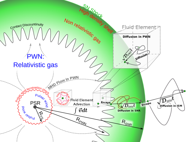
Figure 1: Schematic representation of the main zones and the particle transport mechanisms in composite SNRs.

2 A Model for PWN in the Composite SNR

SNRs that contain a PWN – the so-called composite SNRs – have a specific structure, which is presented schematically in Fig. 1. The part that is referred to as PWN is filled with relativistic particles that originate from the pulsar. Bulk velocities in this region can be relativistic, in particular, close to its inner boundary, which is the pulsar wind TS. The contact discontinuity (CD) bounds the PWN from outside. The plasma velocities close to the CD are nonrelativistic. Thus, an efficient advection in PWNe is most likely limited by the inner region of the nebula, which may, however, extend significantly beyond the TS. In contrast to advection, the diffusive transport is not constrained by any specific hydrodynamic region. It allows particles to escape from the PWN to the SNR region. Apparently, the diffusion coefficients in PWN and SNR may differ significantly. Similarly, the advection in the SNR is limited by the region between the CD and the SN shock. In this region, the flow velocities are small ($\sim 10^{4}\rm\,km\,s^{-1}$). The diffusion in the SNR leads to the particle escape. The high-energy particles from the SNR can penetrate PWN or eventually escape to the ISM. In the ISM, the diffusion proceeds at a rate corresponding to the diffusion of the galactic cosmic rays (CRs). Note that in the Galactic disk the CR diffusion is much (orders of magnitude) faster compared to the diffusion in the Bohm limit. Such a diffusion might be a key element for the formation of extended TeV sources around pulsars (Aharonian, 1995; Abeysekara et al., 2017a). Finally, advection in ISM might be relevant only in the case of high proper velocity of the pulsar.

The evolution and the structure of PWNe are essential for understanding of the origin of radiation seen from these objects. The study of various aspect of PWNe has a long history. Pacini & Salvati (1973a) studied the evolution of the magnetic field at the early epoch of formation of the Crab Nebula and explored the impact of this evolution on the distribution of nonthermal particles and strength of the magnetic field at the present epoch (Pacini & Salvati, 1973b). The impact of the dynamics of PWNe on a self-gravitating shell was investigated by Maceroni et al. (1974). Later on, Reynolds & Chevalier (1984) proposed a comprehensive model describing the dynamics of evolution of the PWNe in the SNR (see also Bucciantini et al., 2011). In some other studies, the structure of PWNe within a slowly expanding SNR shell has been explored (Rees & Gunn, 1974). This approach has been developed into a detailed 1D magnetohydrodynamic (MHD) model for the Crab Nebula (Kennel & Coroniti, 1984a, b). The latter describes remarkably well the broadband SED of the Crab Nebula from the optical to soft gamma-ray band through the synchrotron radiation and in the VHE band through the IC scattering of electrons (Atoyan & Aharonian, 1996). Finally, in recent years different aspects of the PWN evolution have been addressed through 2D and 3D (M)HD numerical simulations. In particular, a significant progress has been achieved in the modeling of X-ray morphology caused by the pulsar wind anisotropy (see, e.g., Del Zanna et al., 2004; Porth et al., 2014) and by the reverse shock at the later stages of evolution of the PWN (see, e.g., Kolb et al., 2017).

In this paper, we develop an analytical model to describe the dynamics of evolution of the anomalously extended PWNe. Generally, the studies of PWNe silently assume that the dominant contribution to the energy of a composite SNR is provided by the supernovae (SN) explosion. Indeed, the total deposited energy by one of the currently most powerful pulsars, the Crab pulsar, is estimated as $3\times 10^{50}\mathrm{erg}$, which is significantly smaller than the energy transferred to the ejecta at the SN Type II explosion (Reynolds & Chevalier, 1984). If the SNR energy is dominated by the SN explosion, then Sedov’s solution provides a rather accurate estimate of the source size. In this case, extended PWNe, with a size significantly exceeding $10\rm\,pc$, are possible only in regions characterized by an extremely low density of the ISM (e.g., de Jager & Djannati-Ataï, 2009). The required density, as low as $n_{\textsc{ism}}\approx 10^{-3}\ \rm cm^{-3}$, is not typical for the conventional regions of the ISM in the Galactic Plane. Moreover, in the specific case of HESS J1825$-$137 (catalog ), it is not supported by observations that revealed dense molecular clouds in the vicinity of HESS J1825$-$137 (catalog ) (Voisin et al., 2016). Below, we explore whether the problem can be resolved (or at least relaxed) in the case of injection of a large amount of energy by the pulsar that dominates over the SN explosion energy. In this case, the dynamics of the system should be similar to Phase IV of the scheme discussed by Reynolds & Chevalier (1984). However, it is important to explicitly account for the dynamics of the ISM involved in the motion. Indeed, the mass of interstellar matter located in a region with a radius $R_{\textsc{snr}}=10\rm\,pc$ can achieve $100M_{\odot}$ for the mean proton density of $1\rm\,cm^{-3}$. We propose a dynamic model that accounts for these two important factors, the dominant pulsar contribution to the dynamics of SNR, and the inertia of the ISM.

2.1 The contribution of pulsar to the overall SN energy

The pulsar rotation losses are determined through the time dependence of its angular velocity: $\dot{E}=I\Omega\dot{\Omega}\,,$ where $\Omega$, $\dot{\Omega}$, and $I$ are the pulsar angular velocity, its time derivative, and the moment of inertia of the neutron star (NS), respectively. The later is calculated using the relation

$$I\simeq 10^{45}{\,\rm\,g\,cm^{2}}\,\left[\left({M_{\textsc{psr}}\over 1.4M_{\odot}}\right)\left({R_{\textsc{psr}}\over 10\rm\,km}\right)^{2}\right]\,.$$ (1)

It is conventionally assumed that the change of the angular velocity is determined by the braking index, $n$: $\dot{\Omega}\propto\Omega^{n}\,.$ If the time $t^{\prime}=0$ corresponds to the present epoch, the pulsar power evolves with time as

$$L_{\rm sd}(t)={L_{p}\over\left(1+t^{\prime}/t_{0}^{\prime}\right)^{{n+1\over n-1}}}\,.$$ (2)

Here, $\Omega_{p}$ and $\dot{\Omega}_{p}$ are the current angular velocity and the angular acceleration, respectively. The characteristic time, $t_{0}^{\prime}$ is determined by the pulsar characteristic age, $\tau=-\Omega_{p}/2\dot{\Omega}_{p}$, and the braking index,

$$t_{0}^{\prime}={2\tau\over(n-1)}\,.$$ (3)

In the above treatment, the pulsar birth epoch, $-t_{0}^{\prime}<t_{\rm b}^{\prime}<0$, is uncertain. For almost all pulsars, the measured values of the braking index, $n$, vary between $1$ and $3$ (Lyne et al., 1993; Boyd et al., 1995; Lyne et al., 1996; Livingstone et al., 2007; Weltevrede et al., 2011; Livingstone et al., 2011; Roy et al., 2012), with two exceptions: PSR J1734$-$3333 ($n=0.9\pm 0.2$, Espinoza et al., 2011) and PSR J1640$-$4631 ($n=3.15\pm 0.03$, Archibald et al., 2016). Thus, the true age of the pulsar can exceed, by a factor $>5$, the characteristic age, $\tau$ (see, e.g., de Jager et al., 2005). The birth angular velocity is constrained by the centrifugal breakup limit,

$$\begin{split}\Omega<\Omega_{\rm br}&=\sqrt{GM_{\textsc{psr}}\over R_{\textsc{psr}}^{3}}\\ &=\Omega^{(0)}_{\rm br}\left[\left({M_{\textsc{psr}}\over 1.4M_{\odot}}\right)^{1/2}\left({R_{\textsc{psr}}\over 10\rm\,km}\right)^{-3/2}\right]\,,\\ \end{split}$$ (4)

where $\Omega^{(0)}_{\rm br}=1.4\times 10^{4}{\rm\,s^{-1}}$ corresponds to the breakup velocity for the conventional size of the NS.

The entire energy released by the pulsar since its birth at $t_{b}$ is

$$E=\int\limits_{t_{b}^{\prime}}^{0}dt^{\prime}L_{\rm sd}(t^{\prime})={I\left(\Omega_{\rm b}^{2}-\Omega_{\rm p}^{2}\right)\over 2}\,,$$ (5)

where $\Omega_{b}$ is the birth angular velocity. Unless, the mass and the size of the NS strongly deviate from their conventional values, the breakup constraint limits the total energy released by the pulsar: $E<10^{53}\mathrm{erg}$. Note that $E$ does not depend on the pulsar braking index $n$. This estimate ignores, however, the effects related to the dependence of the moment of inertial on pulsar’s angular velocity. For example, for the velocities close to the breakup limit, the shape of the NS should deviate significantly from the spherical one, resulting in the dependence of $I$ on $\Omega$ (see, e.g., Hamil et al., 2015). The evolution of the NS magnetic field and direction of the magnetic momentum can also lead to a nontrivial dependence of the braking index on time (see, e.g., Hamil et al., 2016; Rogers & Safi-Harb, 2016, 2017). The consideration of these effects is beyond the scope of this paper.

Although a rigid rotating sphere does not, strictly speaking, represent an accurate model for an NS, when its angular velocity is close to the breakup limit, for the sake of simplicity we still use this approximation. In this case, the rotation energy of the pulsar is

$$\begin{split}E_{\textsc{rot}}&={I\Omega_{\rm br}^{2}\over 2}=\frac{1}{5}{GM^{2}\over R}\\ &\simeq 10^{53}\mathrm{erg\,s^{-1}}\left[\left({M_{\textsc{psr}}\over 1.4M_{\odot}}\right)^{2}\left({R_{\textsc{psr}}\over 10\rm\,km}\right)^{-1}\right]\,.\end{split}$$ (6)

The rotation energy constitutes a substantial fraction of the gravitational energy released during the formation of the compact object: $E_{\textsc{grav}}=3E_{\textsc{rot}}$ (here, both estimates ignore the relativistic effects). The formation of a pulsar at SN explosion (see, e.g., Pons et al., 1999) does not a priory exclude that the pulsar gets an angular velocity close to the breakup limit (see, e.g., Heger et al., 2005). Moreover, the bulk of the gravitational energy released during the formation of the compact object is expected to escape with the neutrino emission, and only a tiny fraction, $\sim 1\%$, is transferred to the ejecta, $E_{\textsc{ej}}\sim 10^{51}\mathrm{erg}$. Thus, even if the pulsar rotation energy at its birth is small compared to the breaking limit, it still can exceed the initial kinetic energy of the SN shell. In this case, the dimensions of the SNR and the PWN are determined by the pulsar injection energy.

2.2 Structure of the Composite SNR

The expansion of the PWN determines the evolution of distribution of nonthermal particles and the strength of the magnetic field. Given the relativistic nature of plasma in PWNe, at the stages relevant for the modeling of the present-day nonthermal emission, the hydrodynamic processes in the PWN should proceed in the nearly adiabatic regime. Thus, the internal structure of the nebula can be described analytically. On the other hand, the state of the nonrelativistic shell may depend strongly on its dynamics at earlier stages of the expansion. To explore this evolution, we use a simple dynamic model. The energy of the system is distributed between three components: the kinetic energy of the shell (SNR shell), the internal energy of the nonrelativistic gas in the shell, and the internal energy of the relativistic gas in the nebula. The SNR shell occupies the region between the external boundary of the PWN at $R_{\textsc{pwn}}$, and the SNR radius, $R_{\textsc{snr}}$. The mass of the SNR shell is determined by the gas density of the ISM, $\rho_{\textsc{ism}}$, and the shell radius. The SNR density varies strongly throughout the shell: the mass is concentrated in a thin layer at $R_{\textsc{snr}}$, while the hot nonrelativistic gas fills the remaining part of the shell. The pressure in the hot part of the shell, $P$, is equal to the pressure of the relativistic gas in the PWN. To describe the system, we use a model that includes the following relations:

1. the equation for the energy balance in the nebula,

   $$3{d\,PV_{\textsc{pwn}}\over d\,t}+P{d\,V_{\textsc{pwn}}\over dt}=L_{\rm sd}(t)\,;$$ (7)

2. the equation for the energy balance in the nonrelativistic shell,

   $${d\over d\,t}\left({Mv^{2}\over 2}+\frac{3}{2}{P(V_{\textsc{snr}}-V_{\textsc{pwn}})}\right)=P{d\,V_{\textsc{pwn}}\over d\,t}\,,$$ (8)

   where $v$ is the shell velocity; and

3. the equation of motion,

   $${d\,Mv\over d\,t}=4\pi R_{\textsc{snr}}^{2}P\,.$$ (9)

Let $t$ be the time since the pulsar’s birth:

$$t=t^{\prime}-t_{b}^{\prime}\,,$$ (10)

where the birth epoch is

$$t_{b}^{\prime}=-t_{0}^{\prime}\left[1-\left({\omega\over\tilde{\omega}}\right)^{n-1}\right]\,.$$ (11)

Here, we express the pulsar’s current angular velocity and the velocity at the birth, as fractions of the breakup velocity: $\Omega_{p}=\omega\Omega^{(0)}_{\rm br}$ and $\Omega_{b}=\tilde{\omega}\Omega^{(0)}_{\rm br}$, respectively. The pulsar’s time-dependent spin-down luminosity is

$$L_{\rm sd}(t)={L_{p}\left(\tilde{\omega}/\omega\right)^{(n+1)}\over\left(1+t/t_{0}\right)^{{n+1\over n-1}}}\,,$$ (12)

where the characteristic slow-down time is

$$t_{0}={2\tau\over(n-1)}\left({\omega\over\tilde{\omega}}\right)^{n-1}\,.$$ (13)

Obviously, the present epoch corresponds to $t_{p}=-t_{b}^{\prime}$.

2.2.1 Asymptotic Expansion

For $t\gg t_{0}$, the pulsar injection ceases significantly, and the expansion of the SNR is dominated by the initial energy release. At the initial stage of evolution of the PWN inside the composite SNR does not proceed adiabatically because of the energy injection by the pulsar (see, e.g., Reynolds & Chevalier, 1984) and the severe radiative losses caused by the strong magnetic field (Pacini & Salvati, 1973a). However, at timescales exceeding the pulsar slow-down time, the intensity of the injection by the pulsar ceases. The extension of the nebula results in the reduction of the magnetic field and suppression of radiative losses. Thus, at the later stages of expansion, the PWN should evolve adiabatically. The approach suggested by Zel’dovich & Raizer (1967) can be generalized to describe the evolution of the PWN. The energy of the system consisting of a PWN and the SNR shell is

$$\begin{split}E=&{4\pi\over 3}\left({\rho_{\textsc{ism}}\dot{R}_{\textsc{snr}}^{2}\over 2}R_{\textsc{snr}}^{3}+\right.\\ &\left.{3P\over 2}\left(R_{\textsc{snr}}^{3}-R_{\textsc{pwn}}^{3}\right)+3PR_{\textsc{pwn}}^{3}\right)\,,\end{split}$$ (14)

where the first and second terms describe the contribution from the shell, and the third term characterizes the contribution from the PWN. At later stages, the main contribution to the change of the kinetic energy of the shell is due to the increase of its mass, thus

$$P\propto\rho_{\textsc{ism}}\dot{R}_{\textsc{snr}}^{2}\,.$$ (15)

This allows us to express the energy of the system as

$$E=2\pi P\left(R_{\textsc{pwn}}^{3}+kR_{\textsc{snr}}^{3}\right)\,,$$ (16)

where $k$ is a dimensionless constant. Since the expansion is adiabatic, $PR_{\textsc{pwn}}^{4}=\rm const$. $E$ and $P$ are related as

$$2\pi PR_{\textsc{pwn}}^{4}=aE$$ (17)

or, equivalently,

$$\dot{R}_{\textsc{snr}}^{2}\propto a{E\over\rho_{\textsc{ism}}}R_{\textsc{pwn}}^{-4}\,.$$ (18)

Here, $a$ is a constant of length dimension. The expression for the energy can be simplified as

$$R_{\textsc{pwn}}^{3}\left(R_{\textsc{pwn}}-a\right)=kaR_{\textsc{snr}}^{3}\,.$$ (19)

Combining the above two equations, one obtains

$$\dot{R}_{\textsc{pwn}}\propto a^{5/6}\sqrt{E\over\rho_{\textsc{ism}}}{\left(R_{\textsc{pwn}}-a\right)^{2/3}\over R_{\textsc{pwn}}\left(R_{\textsc{pwn}}-3a/4\right)}\,.$$ (20)

This equation has an analytic solution, which in the asymptotic limit $R_{\textsc{pwn}}\gg a$ is reduced to

$$R_{\textsc{pwn}}\propto a^{1/4}\left({Et^{2}\over\rho_{\textsc{ism}}}\right)^{3/20}\,.$$ (21)

The radius of the PWN allows us to determine the shell radius and the pressure of the SNR (see Eqs. (18) and (15)):

$$R_{\textsc{snr}}\propto\left({Et^{2}\over\rho_{\textsc{ism}}}\right)^{1/5}$$ (22)

and

$$P\propto\rho_{\textsc{ism}}\left({E\over\rho_{\textsc{ism}}t^{3}}\right)^{2/5}\,.$$ (23)

Finally, the ratio of the pulsar spin-down luminosity and the pressure determines the location of the pulsar wind TS:

$$R_{\textsc{ts}}\propto\sqrt{L(t)\over P}\propto t^{\frac{3}{5}-\frac{n+1}{2(n-1)}}\,.$$ (24)

Although the SNR expansion is similar to Sedov’s solution (with a different numerical coefficient), the PWN expands slower with time: $R_{\textsc{pwn}}\propto t^{0.3}$. To infer the details of the SNR expansion, we solve the system of dynamic equations numerically.

2.2.2 Numerical Model

The dynamic equations can be completed with the following phenomenological relations for the shell momentum:

$$Mv=\frac{4\pi}{3}R_{\textsc{snr}}^{3}C_{m}\rho_{\textsc{ism}}{dR_{\textsc{snr}}\over dt}\,,$$ (25)

and the shell kinetic energy

$${Mv^{2}\over 2}=\frac{4\pi}{3}R_{\textsc{snr}}^{3}C_{e}\rho_{\textsc{ism}}\left({d\,R_{\textsc{snr}}\over d\,t}\right)^{2}\,.$$ (26)

Adjusting the constants $C_{m}$ and $C_{e}$ provides a better agreement between the prediction of this simple model and the more accurate numerical treatment. In the case of a strong explosion in a medium with adiabatic index $5/3$, the blast-wave radius and pressure are

$$R_{\textsc{snr}}=\left({\alpha Et^{2}\over\rho_{\textsc{ism}}}\right)^{1/5}$$ (27)

and

$$P=\beta P_{\textsc{snr}}=\frac{3\beta}{4}\rho_{\textsc{ism}}\left({d\,R_{\textsc{snr}}\over d\,t}\right)^{2}\,,$$ (28)

where $\alpha\simeq 1.29$ and $\beta=0.3$ are dimensionless coefficients. The solution of the system correctly reproduces the blast-wave radius and the pressure if one adopts $\displaystyle C_{m}=\frac{3\beta}{2}\approx 0.45$ and $C_{e}=\frac{75}{16\pi\alpha}-\frac{9\beta}{8}\approx 0.82$ (see Appendix A for details). The system of dynamic equations and phenomenological relations can be reduced to the following system:

$$\frac{dP}{dt}=\rho_{\textsc{ism}}\frac{5x^{2}A-8B}{(4+x^{3})R_{\textsc{snr}}}\leavevmode\nobreak\ ,$$ (29)

$$\frac{dR_{\textsc{pwn}}}{dt}=\rho_{\textsc{ism}}\frac{(1-x^{3})A+2xB}{(4+x^{3})P},$$ (30)

$$\frac{dV_{\textsc{snr}}}{dt}=\frac{3{\displaystyle P\over\displaystyle\rho_{\textsc{ism}}}-3C_{m}V_{\textsc{snr}}^{2}}{C_{m}R_{\textsc{snr}}},$$ (31)

$$\frac{dR_{\textsc{snr}}}{dt}=V_{\textsc{snr}}\leavevmode\nobreak\ .$$ (32)

Here, the following notations are used:

$$x=\frac{R_{\textsc{pwn}}}{R_{\textsc{snr}}},\quad A=\frac{L}{4\pi\rho_{\textsc{ism}}R_{\textsc{pwn}}^{2}}\,,$$ (33)

and

$$B=V_{\textsc{snr}}\Big{[}\left(\frac{2C_{e}}{C_{m}}+\frac{3}{2}\right)\frac{P}{\rho_{\textsc{ism}}}-3C_{e}V_{\textsc{snr}}^{2}\Big{]}\,.$$ (34)

Similarly to Sedov’s solution, the inertia of the ISM affects the expansion of the SNR through the dimensionless parameter,

$$s=\sqrt{L_{0}t_{0}^{3}\over\rho_{\textsc{ism}}R_{0}^{5}}\,,$$ (35)

where $R_{0}$, $t_{0}$, and $L_{0}$ are the characteristic spatial, time, and energy scales (see Appendix B for the dimensionless form of the equations).

2.2.3 Initial Conditions

Equations (29) – (32) can be solved numerically, e.g., using the Runge-Kutta method. To proceed with the integration, one needs to define the initial values for $P$, $R_{\textsc{pwn}}$, $R_{\textsc{snr}}$, and $V_{\textsc{snr}}$. The initial values related to the SNR shell should account for the energy transferred at the SN explosion to the ejecta

$$\left.\frac{4\pi}{3}\rho_{\textsc{ism}}R_{\textsc{snr}}^{3}V_{\textsc{snr}}^{2}\right|_{t=0}\simeq E_{\textsc{ej}}\,.$$ (36)

The initial radii of the PWN and SNR should satisfy the obvious condition $R_{\textsc{pwn}}<R_{\textsc{snr}}\ll 1\rm\,pc$. Also, the initial energy of the relativistic gas should be small compared to the characteristic energy injected by the pulsar:

$$\left.\frac{4\pi}{3}R_{\textsc{pwn}}^{3}P\right|_{t=0}\ll L_{b}t_{0}\,.$$ (37)

If these requirements are satisfied, the impact of the initial conditions on the solution of Eqs. (29) – (32) is weak and vanishes once the energy injected by the pulsar significantly exceeds the initial energy. The pulsar initial condition is determined by its birth angular velocity or, equivalently, by its birth epoch for the given braking index; see Eqs. (11) – (13). A typical solution of the system of Equations (29) – (32) is shown in Fig. 2.

More detailed modeling should be performed with numerical simulations of (M)HD equations. This should allow an accurate description of the pressure distribution through the system, which is described in our simplified model by Eq. (28). Detailed HD simulations should also allow us to account for the initial state of the ejecta and resolving its fine structure. The hydrodynamic processes in the SN shell should provide a smaller impact on the size of the system, as compared to the key processes accounted for in our simplified model.

The presence of massive ejecta should significantly slow down the expansion of the system at the earlier stages. This effect can also be instigated with Eqs. (29) – (32), if the ejecta mass is added to the mass terms in Eqs. (25) and (26). As it is shown in Fig. 2, for heavy ejecta with $M_{\textsc{ej}}=30M_{\odot}$, its influence is significant for the first $10^{3}\rm\,yr$ and becomes negligibly small after a few thousands of years.

In the frameworks of the considered dynamic model, the initial state of ejecta has a tiny impact on the final size the nebula. However, the small size of the nebula at the initial stages enhances the rate of the radiative losses significantly. If the radiative losses are dominant, the expansion of the nebula proceeds in a nonadiabatic regime, as it was assumed in Eq. (7), and the nebula may not be able to push the SN shell as efficient as predicted by Eqs. (29) – (32).

The rate of radiative losses is determined by the composition of the pulsar wind and its magnetization. Conventionally, one assumes that electrons/positrons are the predominant ingredients of pulsar winds. There is a significant uncertainty in the value of the electron mean Lorentz factor, $\Gamma$. It can range from a few hundred (similar to the pulsar wind Lorentz factor close to the light cylinder) to a value of $\sim 10^{6}$ anticipated in the Crab Nebula. The magnetic field tends to the equitation with the gas pressure; however, initially, the magnetic field can be weak, with the magnetic pressure being just a few percent of the gas pressure.

To compare the rate of synchrotron and adiabatic cooling, we assume that the magnetic pressure is equal to a fraction of the gas pressure: $P_{\textsc{b}}=(B^{2}/8\pi)=\varkappa_{\textsc{b}}P$. The ratio of the losses is

$$\varkappa={\dot{\gamma}_{\rm syn}\over\dot{\gamma}_{\rm ad}}=-{\frac{4}{3}c\sigma_{\textsc{t}}P_{\textsc{b}}\Gamma^{2}\over\frac{1}{3}\Gamma{d{\rm ln}n\over dt}}=\Pi\varkappa_{\textsc{b}}\Gamma\,.$$ (38)

The function $\Pi$ depends only on the hydrodynamic properties of the nebula, thus can be evaluated with the model described by Eqs. (29) – (32). In Fig. 3 the parameter $\Pi$ is shown as a function of time since the pulsar birth. For large values, $\Pi>10^{-2}$, the nebula expansion most likely proceeds in a nonadiabatic regime, thus the obtained solution has limited applicability. A massive ejecta causes the nonadiabatic regime at the initial stage. Depending on the braking index, the transition to the adiabatic regime should occur between tens or hundreds of years. In the case of large values of the braking index, $n\sim 3$, the pulsar slow-down occurs on a timescale shorter than the duration of the nonadiabatic phase, thus the solution obtained with Eqs. (29) – (32) may overestimate the size of the PWN. In contrast, for the small values of the braking index, $n\sim 1.5$, the pulsar slow-down takes significantly longer than the duration of the nonadiabatic phase, thus the obtained solution should provide a meaningful estimate on the size of the nebula.

Radiative cooling may affect the dynamics of the nonrelativistic shell. Matter emissivity depends on its temperature, the abundances of chemical elements, and the density. Several simple approximations for the radiative losses have been obtained by a number of authors (see, e.g., Koldoba et al., 2008, and references therein). The model described by Eqs. (25 - 32) does not allow an accurate evaluation of the radiative cooling since such an estimate requires a detailed information about the density and temperature distributions in the nonrelativistic shell. Thus, to address the radiative cooling we compute a fraction of energy radiated in the case of Sedov’s explosion. Accounting for the density and temperature distributions, the radiated energy fraction is

$$\begin{split}\frac{\Delta E}{E}<\quad&8\times 10^{-3}\left({n_{\textsc{ism}}\over 1\rm\,cm^{-3}}\right)^{1.64}\times\\ &\left({E\over 10^{51}\rm\,erg}\right)^{-0.64}\left({t\over 10\rm\,kyr}\right)^{2.92}\,.\end{split}$$ (39)

The emitted energy, $\Delta E$, corresponds to radiative losses in the entire shell integrated from the explosion moment to $t$ (see Appendix C for detail). From this estimate one can conclude that for $n_{\textsc{ism}}\sim 1\rm\,cm^{-3}$ and $E\gg 10^{51}\rm\,erg$ the shock should remain nonradiative for the entire evolution of the system, $t\leq 10^{5}\rm\,yr$.

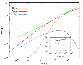
Figure 2: Numerical solution of the system of Equations (29) – (32) together with lines showing the asymptotic behavior as predicted by Equations (22), (21), and (24). The pulsar angular velocity and the braking index are assumed to be ${\tilde{\omega}}=0.5$ and $n=1.5$, respectively. The calculation is performed for the ISM with a mean gas number density ${\bar{n}}_{\textsc{ism}}=1\rm\,cm^{-3}$. Thin line shows a solution of a system similar to Eqs. (29) – (32), where the mass of the shell has an additional contribution of $30M_{\odot}$ ejecta. The inclusive plot shows the dependence of the SNR shock velocity.

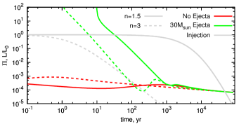
Figure 3: Hydrodynamic parameter $\Pi$ that determines the ratio of the synchrotron and adiabatic losses, $\varkappa$, through Eq. (38). Calculations are performed for two values of the braking index: $n=1.5$ (solid lines) and $n=3$ (dashed lines). A heavy ejecta ($M_{\textsc{ej}}=30M_{\odot}$) significantly enhances the rate of radiative cooling at the early stage of expansion. Gray lines show the normalized rate of injection by the pulsar.

3 Implications for HESS J1825$-$137 (catalog )

3.1 Size of the nebula

For the distance to the source of HESS J1825$-$137 (catalog ) of 4 kpc (based on dispersion measure using the models for Galactic electrons by Taylor & Cordes, 1993; Cordes & Lazio, 2002), the measured angular size of the latter corresponds to the 70 pc linear size of the gamma-ray production region. Although the gamma-ray image deviates from the spherically symmetric shape; below for simplicity we will assume that the radius of the source is 35 pc. The detection of a H$\alpha$ rim at a distance of $R_{\textsc{obs}}=120\rm\,pc$ from the pulsar PSR J1826-1334 has been interpreted as a signature of the progenitor SNR (see Stupar et al., 2008; Voisin et al., 2016). As illustrated in Fig. 4, in the case of an ISM density gradient, the measured radius does not coincide with the radius, $R_{\textsc{snr}}$. If the pulsar is still located inside the SNR then the SNR radius cannot be significantly smaller than the observed distance: $R_{\textsc{snr}}>R_{\textsc{obs}}/2$. Thus, with a factor of two uncertainty one can estimate the radius based on Sedov’s solution:

$$\begin{split}R_{\textsc{snr}}&\simeq\left({1.3E_{\textsc{ej}}t_{p}^{2}\over\rho_{\textsc{ism}}}\right)^{1/5}\\ &\sim 12\left({E_{\textsc{ej}}\over 10^{51}\mathrm{erg}}\right)^{1/5}\left({t_{p}\over 10\rm\,kyr}\right)^{2/5}\left({n_{\textsc{ism}}\over 1\rm\,cm^{-3}}\right)^{-1/5}\rm\,pc\,,\\ \end{split}$$ (40)

where $\rho_{\textsc{ims}}=n_{\textsc{ism}}\,m_{p}$ are the density, the hydrogen number density, and the proton mass, respectively. Thus, the SNR shell can be located at the distance of $R_{\textsc{obs}}\sim 120$ pc, provided that the following condition is fulfilled:

$$\left({t_{p}\over 10\rm\,kyr}\right)^{2}\left({E_{\textsc{ej}}\over 10^{51}\mathrm{erg}}\right)\left({{\bar{n}}_{\textsc{ism}}\over 1\rm\,cm^{-3}}\right)^{-1}>3\times 10^{3}\,,$$ (41)

where the numerical value corresponds to $R_{\textsc{snr}}=R_{\textsc{obs}}/2\simeq 60\rm\,pc$. The ejecta energy at SN type II is constrained by $E_{\textsc{ej}}\simeq 3\times 10^{51}\mathrm{erg}$, while the age of the source is limited by $t_{p}<100\,\rm kyr$ (for $n\simeq 1.5$). Thus, Sedov’s solution is consistent with the observed size of the SNR when ${\bar{n}}_{\textsc{ism}}<0.1\rm\,cm^{-3}$. Note that de Jager & Djannati-Ataï (2009) derived somewhat smaller upper limit for ${\bar{n}}_{\rm ism}$ assuming the braking index $n=2$. This upper limit seems to be below the typical density of the interstellar gas in the Galactic Plane. Moreover, Voisin et al. (2016) reported the presence of several molecular clouds in the small angular proximity to the nebula with an average number density $n_{\rm c}\sim 10^{3}\,\rm cm^{-3}$ and characteristic size $r_{\rm c}\sim 10\rm\,pc$. It is likely that one of these clouds is responsible for the anisotropic expansion of the nebula, thus it should be located close to the nebula. The gas density in molecular clouds is expected to follow the King’s profile:

$$\rho={\rho_{\rm c}\over(1+r/r_{\rm c})^{2}}\,.$$ (42)

Thus, the density to the south of the pulsar can hardly be as low as it is required by Sedov’s solution. Instead, it should be comparable to the upper limit of $n_{\textsc{ism}}\sim 4\rm\,cm^{-3}$ obtained by Voisin et al. (2016).

To avoid this problem, we suggest an alternative scenario in which the energy injection by the pulsar dominates over the kinetic energy of the ejecta. This scenario has an advantage since it offers significantly larger available energy.

The energy for the source expansion is transferred through the PWN, which evolves adiabatically, and the energy, consumed for the expansion, is determined by the volumes of the PWN and SNR. Thus, their sizes should be measured neither from the SN explosion point nor from the present pulsar location. Instead one should use, as a starting point, the geometrical center of the current structure.

Below, we adopt the following requirements to be met by the 1D model: $R_{\textsc{ts}}\sim 0.03\rm\,pc$, $R_{\rm pwn}\sim 35\rm\,pc$, and $R_{\textsc{snr}}>R_{\textsc{obs}}/2=60\rm\,pc$. As it follows from Figure 4, the 3D structure of the system implies a large uncertainty for the relation between $R_{\textsc{snr}}$ and $R_{\textsc{obs}}$. This can be consistently resolved only with realistic 3D numerical simulations, which is beyond the scope of this paper.

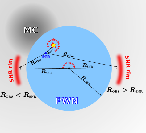
Figure 4: Arrangement and characteristic distances in the 1D model. In the frameworks of 1D model, all the relevant distances, $R_{\textsc{pwn}}$ and $R_{\textsc{snr}}$, should be measured from the geometrical center of the nebula. A nearby molecular cloud (indicated as “MC”) can render an anisotropic expansion of the system.

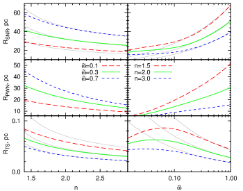
Figure 5: Present-day radii of the SNR (top panels), PWN (middle panels), and pulsar wind TS (bottom panels) as functions of the pulsar braking index $n$ (left panels) and pulsar birth angular velocity (right panels). In the left panels, the calculations are performed for three values of the pulsar angular velocity at its birth: $\tilde{\omega}=0.1$, $0.3$, and $0.7$. These numbers correspond to 1%, 10%, and 50% of the pulsar gravitational energy. In the right panels, the calculations are performed for three values of the braking index $n=1.5$, $2$, and $3$. The adopted number density of the surrounding gas is ${{\bar{n}}_{\textsc{ism}}}=1\rm\,cm^{-3}$. The thin gray lines show analytic approximations given by Eqs. (43) and (44).

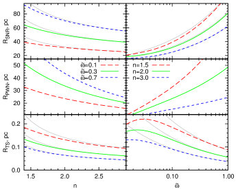
Figure 6: Same as in Fig. 6 but for ${{\bar{n}}_{\textsc{ism}}}=0.1\rm\,cm^{-3}$.

For the present-day spin-down luminosity and the characteristic age of the pulsar, the size of the the composite SNR is determined by three parameters: the braking index $n$, the initial rotation velocity $\tilde{\omega}$, and the density of the surrounding medium ${\bar{\rho}}_{\textsc{ism}}$. The braking index and the initial rotation velocity determine the age of the system through Eq. (11), the birth spin-down luminosity through Eq. (12), and the initial slow-down time through Eq. (13).

The results of the calculation of the present-day size are shown in Figs. 5 and 6. These calculations allow determination of the numerical coefficients for the asymptotic expressions given by Eqs. (22) and (24):

$$R_{\textsc{snr}}\simeq 52\left({\tilde{\omega}^{2}\over(n-1)^{2}\rho_{0}}\right)^{1/5}\rm\,pc\,,$$ (43)

$$R_{\textsc{ts}}\simeq 0.028\left({(n-1)^{6}\tilde{\omega}^{4}\rho_{0}^{3}}\right)^{-1/10}\rm\,pc\,,$$ (44)

where $\rho_{0}={{\bar{\rho}}_{\textsc{ism}}}/(m_{p}\rm\,cm^{-3})$. For ${\tilde{\omega}}>0.1$ and $n>1.5$, these approximations are rather accurate; it can be checked from the comparison of the results of the numerical calculations shown in Figs. 5 and 6. For small values of $\tilde{\omega}\leq 0.1$, the pulsar contribution to the overall energy budget becomes comparable to the assumed initial energy of the SNR shell, which was ignored when deriving these expressions. Also, it is assumed that the bulk of the pulsar rotation energy is promptly released at the initial phase. This assumption violates for small values of the braking index $n$. Finally, we note that because of the presence of parameter $a$ in Eq. (21), the size of the PWN cannot be described by an approximate formula similar to Eqs. (43) and (44). A comparison of Eq. (44) with the TS radius implies that the density of the medium should be rather high, ${\bar{n}}_{\textsc{ism}}\sim 1\rm\,cm^{-3}$. For this high medium density, the SNR and PWN can be sufficiently extended if ${\tilde{\omega}}>0.5$ and $n\leq 2$ as shown in Fig. 5.

4 Summary

The total energy released at an SN type II explosion, $10^{53}\mathrm{erg}$, exceeds, by two orders of magnitude, the energy transferred to the ejecta, $E_{\textsc{ej}}\sim 10^{51}\mathrm{erg}$. The bulk of energy escapes with the neutrino emission. Typically, the pulsar rotation energy is small compared to the ejecta energy. However, it cannot be excluded that at some circumstances the pulsar can receive a larger fraction of the explosion energy. When it becomes comparable to the kinetic energy of the ejecta, the sizes of both the SNR and the PWN can significantly deviate from Sedov’s solution. To illustrate the implication of this scenario, we considered a specific case of HESS J1825$-$137 (catalog ), a very extended and bright in VHE gamma-rays PWN (Aharonian et al., 2006; Pavlov et al., 2008; Mitchell et al., 2017b, a; H.E.S.S. Collaboration et al., 2018b). The X-ray and gamma-ray observations of HESS J1825$-$137 (catalog ) show that the shape of the nebula deviates from the spherically symmetric geometry. Thus, the 1D model described in Sec. 2 has limited capability for accurate quantitative predictions. However, in the framework of the suggested scenario, the hydrodynamic processes evolve differently from the conventional situations, and the 1D model should provide a correct estimate for the energy required for the PWN/SNR inflation. In the framework of the scenario, the pressure in the PWN is the main driving force of the SNR expansion. Independently on symmetry of the system and dimension of the used model, the PWN is nearly isobaric, thus the radius of the pulsar wind TS provides an observational constraint for the pressure in the nebula. Therefore, we adopt the following requirement: the present-day pressure in the nebula should be consistent with the pulsar wind TS located at $R_{\textsc{ts}}\sim 0.03\rm\,pc$ from the pulsar (Van Etten & Romani, 2011). The 1D model allows us to obtain the radii of the SNR, PWN, and pulsar wind TS as functions of three key model parameters: density of the ISM, pulsar braking index, and the initial angular velocity of the pulsar. In the framework of this model, it is possible to reproduce the three key properties of the system: $R_{\textsc{snr}}\geq 60\rm\,pc$, $R_{\textsc{pwn}}\simeq 35\rm\,pc$, and $R_{\textsc{ts}}\simeq 0.03\rm\,pc$, provided that (i) the pulsar obtains, at its birth, a significant fraction of the explosion energy (${\tilde{\omega}}\geq 0.5$), and (ii) the braking index is small, $n\leq 2$. The conventional Sedov-like solution implies a low density of the ISM, ${\bar{n}}_{\textsc{ism}}<0.1\rm\,cm^{-3}$. In contrast, the model proposed in this paper requires a rather dense environment, ${\bar{n}}_{\textsc{ism}}\sim 1\rm\,cm^{-3}$. This agrees with the presence of dense molecular clouds reported in the vicinity of the source (Voisin et al., 2016). What concerns the requirement for the pulsar braking index, $n\leq 2$, is that it is small compared to the value measured for the Crab pulsar (Lyne et al., 1993), but it matches both the old (e.g., Vela; $n=1.4\pm 0.2$, Lyne et al., 1996) and young (e.g., J1833$-$1034; $n=1.8569\pm 0.001$, Roy et al., 2012) pulsars.

Equations (43) and (44) allow us to estimate the model parameters based on the requirement to reproduce the observed sizes of the SNR and the position of the TS. For example, if the true size of the SNR approaches $120\rm\,pc$, then the scenario suggested in this paper requires $(n-1)\rho_{0}^{1/2}\simeq 0.43$ (for $R_{\textsc{ts}}\simeq 0.03\rm\,pc$). Formally, this relation can be easily fulfilled. However, one should also account for the required birth angular velocity: $\tilde{\omega}\simeq 3.5$. Such a high value implies (see Eq. (6)) that the pulsar physical parameters significantly deviates from the conventional values.

The most demanding requirement for the suggested scenario is the initial rotation energy of the pulsar. Our simulations require fast angular velocity at the birth, ${\tilde{\omega}}\geq 0.5$, which implies a very small initial rotation period, $P_{\rm b}\leq 1\rm\,ms$. This translates to a lower limit on the birth spin-down luminosity

$$L_{\rm b}>3\times 10^{41}\mathrm{erg\,s^{-1}}\,,$$ (45)

for the braking index and the initial angular velocity: $n=1.5$ and ${\tilde{\omega}}=0.5$, respectively. The requirement for the very fast initial rotation may seem an extreme assumption. However, as Heger et al. (2005) have shown, the differential rotation in a massive progenitor should result in the formation of a rapidly rotating pulsar. For example, numerical simulations predict the birth of a pulsar with $P_{\rm b}=3\rm\,ms$ for a $35M_{\odot}$ progenitor star. Thus, the option of an initially very fast rotating pulsar a priori cannot be excluded. It should be considered along with the conventional scenario that provides an explanation of the very large size of HESS J1825$-$137 (catalog ) assuming an extremely low density environment surrounding the source.

Appendix A Numerical Model for the SN Explosion

If the injection of energy by the PWN is sufficiently small to have an impact on the dynamics of the SNR, the dynamic equations consist of the requirement of energy conservation:

$$\frac{d}{dt}\left(\frac{Mv^{2}}{2}+\frac{3PV_{\textsc{snr}}}{2}\right)=0\leavevmode\nobreak\ .\,;$$ (A1)

and the Second Newton law:

$$\frac{dMv}{dt}=4\pi R_{\textsc{snr}}^{2}P\leavevmode\nobreak\ .$$ (A2)

Here, it is adopted that the shell mass is concentrated close to the blast-wave. Eqs. (A1) and (A2) can be completed with empirical relations for the shell’s momentum and kinetic energy:

$$Mv=C_{m}\rho_{\textsc{ism}}\frac{4\pi R_{\textsc{snr}}^{3}}{3}\frac{dR_{\textsc{snr}}}{dt},\leavevmode\nobreak\ \leavevmode\nobreak\ \leavevmode\nobreak\ \leavevmode\nobreak\ \frac{Mv^{2}}{2}=C_{e}\rho_{\textsc{ism}}\frac{4\pi R_{\textsc{snr}}^{3}}{3}\left(\frac{dR_{\textsc{snr}}}{dt}\right)^{2}\leavevmode\nobreak\ .$$

The solution of the hydrodynamics equation allows us to find numerically the coefficients for Sedov’s self-similar solution. Namely, the blast-wave radius, $R_{\textsc{snr}}$, and pressure at explosion point, $P_{c}$, are

$$R_{\textsc{snr}}=\left(\frac{\alpha Et^{2}}{\rho_{\textsc{ism}}}\right)^{1/5},\leavevmode\nobreak\ \leavevmode\nobreak\ \leavevmode\nobreak\ \leavevmode\nobreak\ P=\beta P_{c}=\frac{3\beta}{4}\rho_{\textsc{ism}}\dot{R}_{\textsc{snr}}^{2}\leavevmode\nobreak\ ,$$

where $E$ and $P$ are the explosion energy and pressure behind the blast-wave. For polytropic gas with $\gamma=5/3$, the numerical coefficients are $\alpha\approx 1.29,\leavevmode\nobreak\ \beta\approx 0.3$. Eq. (A1) can be integrated, yielding

$$\frac{Mv^{2}}{2}+\frac{3PV}{2}=\frac{4\pi}{3}\rho_{\textsc{ism}}C_{e}R_{\textsc{snr}}^{3}\dot{R}_{\textsc{snr}}^{2}+\frac{4\pi}{3}R_{\textsc{snr}}^{3}\frac{3P}{2}=\frac{4\pi}{3}R_{\textsc{snr}}^{3}\left(\rho_{\textsc{ism}}C_{e}\dot{R}_{\textsc{snr}}^{2}+\frac{3P}{2}\right)=E\leavevmode\nobreak\ .$$ (A3)

In turn, Eq. (A3) is fulfilled if

$$\dot{R}_{\textsc{snr}}=AR_{\textsc{snr}}^{-3/2}\leavevmode\nobreak\ ,$$ (A4)

$$P=BR_{\textsc{snr}}^{-3}\leavevmode\nobreak\ .$$ (A5)

Note that

$$\frac{4\pi}{3}\left(\rho_{\textsc{ism}}C_{e}A^{2}+\frac{3B}{2}\right)=E\leavevmode\nobreak\ .$$ (A6)

Solving Eq. (A4) one obtains $\displaystyle R_{\textsc{snr}}=\left(\frac{5At}{2}\right)^{2/5}=\left(\frac{\alpha Et^{2}}{\rho_{\textsc{ism}}}\right)^{1/5},\leavevmode\nobreak\ \leavevmode\nobreak\ \leavevmode\nobreak\ \leavevmode\nobreak\ \frac{25A^{2}}{4}=\frac{\alpha E}{\rho_{\textsc{ism}}}$, which yields in $\displaystyle A^{2}=\frac{4\alpha E}{25\rho_{\textsc{ism}}}$. Changing variables in Eq. (A2) as $R_{\textsc{snr}},\leavevmode\nobreak\ \leavevmode\nobreak\ \leavevmode\nobreak\ \leavevmode\nobreak\ dR_{\textsc{snr}}=Ddt,\leavevmode\nobreak\ \leavevmode\nobreak\ \leavevmode\nobreak\ \leavevmode\nobreak\ D=\dot{R}_{\textsc{snr}}$, one obtains

$$\frac{4\pi}{3}\rho_{\textsc{ism}}C_{m}\frac{dR_{\textsc{snr}}^{3}D}{dR_{\textsc{snr}}}=4\pi\frac{R_{\textsc{snr}}^{2}P}{D}\leavevmode\nobreak\ .$$ (A7)

Substituting in Eq. (A7) one derives that $\displaystyle\frac{\rho_{\textsc{ism}}C_{m}A^{2}}{2}=B$. Thus, the following chain of equations should be satisfied

$$\frac{P}{\dot{R}_{\textsc{snr}}^{2}}=\frac{3\beta\rho_{\textsc{ism}}}{4}=\frac{B}{A^{2}}=\frac{\rho_{\textsc{ism}}C_{m}}{2}\leavevmode\nobreak\ .$$

This implies $\displaystyle C_{m}=\frac{3\beta}{2}$. Eq. (A6) can be simplified as

$$\frac{3E}{4\pi}=\rho_{\textsc{ism}}C_{e}A^{2}+\frac{3C_{m}\rho_{\textsc{ism}}A^{2}}{4}=\rho_{\textsc{ism}}\left(C_{e}+\frac{3C_{m}}{4}\right)\frac{4\alpha E}{25\rho_{\textsc{ism}}}=\left(C_{e}+\frac{3C_{m}}{4}\right)\frac{4\alpha E}{25}\leavevmode\nobreak\ ,$$ (A8)

and, consequently,

$$\frac{3}{4\pi}=\left(C_{e}+\frac{3C_{m}}{4}\right)\frac{4\alpha}{25}\leavevmode\nobreak\ .$$ (A9)

This allows us to obtain the coefficient as

$$C_{e}=\frac{75}{16\pi\alpha}-\frac{3C_{m}}{4}=\frac{75}{16\pi\alpha}-\frac{9\beta}{8}\leavevmode\nobreak\ .$$ (A10)

This means that the dynamic model can correctly reproduce the size of the SNR and the pressure of the gas at the explosion point if $\displaystyle C_{m}=\frac{3\beta}{2}\approx 0.45,\leavevmode\nobreak\ \leavevmode\nobreak\ C_{e}=\frac{75}{16\pi\alpha}-\frac{9\beta}{8}\approx 0.82$. The parameters $\alpha\approx 1.29$ and $\beta\approx 0.3$ are the numerical coefficients for Sedov’s solution in polytropic gas with $\gamma=5/3$. The obtained values for $C_{e}$ and $C_{m}$ are also used in the dynamic model for the composite “PWN+SNR” model.

Appendix B Dimensionless Form of the Equations

The dimensionless equations that determine the expansion of the SNR and PWN are

$$\frac{dp}{d\tau}=\frac{5x^{2}a-8(b_{1}+b_{2}/s)}{(4+x^{3})r_{\textsc{snr}}}\leavevmode\nobreak\ ,$$ (B1)

$$\frac{dr_{\textsc{pwn}}}{d\tau}=\frac{(1-x^{3})a+2x(b_{1}+b_{2}/s)}{(4+x^{3})p},$$ (B2)

$$\frac{dv_{\textsc{snr}}}{dt}=\frac{{\displaystyle 3ps\over\displaystyle C_{m}}-3v_{\textsc{snr}}^{2}}{r_{\textsc{snr}}},$$ (B3)

$$\frac{dr_{\textsc{snr}}}{d\tau}=v_{\textsc{snr}}\leavevmode\nobreak\ .$$ (B4)

Here, the characteristic time, space and energy scales—$t_{0}$, $R_{0}$, and $L_{0}$—define the dimensionless variables $t=t_{0}\tau$, $R_{{\textsc{snr}}/pwn}=R_{0}r_{{\textsc{snr}}/pwn}$, $V_{\textsc{snr}}=v_{\textsc{snr}}(R_{0}/t_{0})$, $P={L_{0}t_{0}\over R_{0}^{3}}p$, $\displaystyle x=\frac{r_{\textsc{pwn}}}{r_{\textsc{snr}}}$, $a=\frac{L}{4\pi L_{0}r_{\textsc{pwn}}^{2}}$, $b_{1}=v_{\textsc{snr}}p\left(\frac{2C_{e}}{C_{m}}+\frac{3}{2}\right)$, and $b_{2}=-C_{e}v_{\textsc{snr}}^{3}$. Similarly to Sedov’s solution, a dimensionless parameter

$$s={L_{0}t_{0}^{3}\over\rho_{\textsc{ism}}R_{0}^{5}}$$ (B5)

accounts for the inertia of the ISM.

Appendix C Radiation Cooling for Sedov’s Solution

Thermal radiation may affect properties of the nonrelativistic shock. The nonrelativistic shell should be quite unhomogeneous and the physical conditions in the shell undergo substantial changes during the SNR evolution. Since the thermal emission coefficient depends nonlinearly on the plasma density and temperature, one should utilize a precise spatial–time description of the nonrelativistic gas to address the thermal cooling accurately. The model suggested in this paper shares much in common with the classic Sedov solution, especially in regard to the evolution of the nonrelativistic gas. Thus, to evaluate the importance of the thermal cooling, we calculate a fraction of radiated energy for a self-similar Sedov’s explosion.

We adopt the adiabatic index of ideal nonrelativistic gas to be $\gamma=5/3$. Temperature and density in the self-similar solution depend on the spatial coordinate as

$$T=T_{s}F(\xi),\leavevmode\nobreak\ \leavevmode\nobreak\ \leavevmode\nobreak\ n=n_{s}G(\xi)\,,$$ (C1)

where $\xi={r/R_{\textsc{snr}}(t)}$ is the dimensionless radius. Functions in Eq. (C1) selected to satisfy the following conditions: $F(1)=G(1)=1$. The shock-front values of density and temperatures are

$$n_{s}=4n_{\textsc{ism}},\leavevmode\nobreak\ \leavevmode\nobreak\ \leavevmode\nobreak\ \leavevmode\nobreak\ T_{s}=\frac{p_{s}}{2k_{B}n_{s}}=\frac{3m_{p}}{200k_{B}}\Big{(}\frac{R_{\textsc{snr}}}{t}\Big{)}^{2}\,,$$ (C2)

where the shock-front pressure is

$$p_{s}=\frac{3\rho_{0}}{4}\Big{(}\frac{2R_{\textsc{snr}}}{5t}\Big{)}^{2}=\frac{3m_{p}n_{\textsc{ism}}}{25}\Big{(}\frac{R_{\textsc{snr}}}{t}\Big{)}^{2}\,.$$ (C3)

Thermal radiation losses are determined by the cooling function $\Lambda$ as

$$\begin{split}\frac{dE}{dt}&=\int\limits_{0}^{R_{\textsc{snr}}}n_{\textsc{h}}n_{e}\Lambda(T)4\pi r^{2}dr=4\pi A\int\limits_{0}^{R_{\textsc{snr}}}n^{2}T^{-a}r^{2}dr=4\pi AR_{\textsc{snr}}^{3}n_{s}^{2}T_{s}^{-a}\int\limits_{0}^{1}G(\xi)^{2}F(\xi)^{-a}\xi^{2}d\xi\\ &=4\pi AR_{\textsc{snr}}^{3}16n_{\textsc{ism}}^{2}\Big{(}\frac{3m_{p}}{200k_{B}}\Big{)}^{-a}\Big{(}\frac{R_{\textsc{snr}}}{t}\Big{)}^{-2a}\int\limits_{0}^{1}G^{2}F^{-a}\xi^{2}d\xi\,,\end{split}$$ (C4)

where one assumed hydrogen gas, i.e., the electron density, $n_{e}$, is equal to the proton density, $n_{\textsc{h}}$. The TS radius is

$$R_{\textsc{snr}}=\Big{(}\frac{Et^{2}}{m_{p}n_{\textsc{ism}}}\Big{)}^{1/5}\,,$$ (C5)

and the cooling function was approximated as $\Lambda=AT^{-a}$. This results in the following thermal radiation losses:

$$\begin{split}\frac{dE}{dt}&=64\pi A\Big{(}\frac{Et^{2}}{m_{p}n_{\textsc{ism}}}\Big{)}^{3/5}n_{\textsc{ism}}^{2}\Big{(}\frac{3m_{p}}{200k_{B}}\Big{)}^{-a}\Big{(}\frac{E}{m_{p}n_{\textsc{ism}}}\Big{)}^{-2a/5}t^{6a/5}\int\limits_{0}^{1}G^{2}F^{-a}\xi^{2}d\xi\\ &=CA\Big{(}\frac{E}{m_{p}}\Big{)}^{(3-2a)/5}n_{\textsc{ism}}^{1.4+2a/5}\Big{(}\frac{3m_{p}}{200k_{B}}\Big{)}^{-a}t^{6(1+a)/5}\,,\end{split}$$ (C6)

where $C=64\pi\int\limits_{0}^{1}G^{2}F^{-a}\xi^{2}d\xi$ is a constant. According to Hollenbach & McKee (1979), one can adopt $a=0.6$, thus the thermal cooling is

$$\frac{dE}{dt}=CA\Big{(}\frac{E}{m_{p}}\Big{)}^{0.36}n_{\textsc{ism}}^{1.64}\Big{(}\frac{3m_{p}}{200k_{B}}\Big{)}^{-0.6}t^{1.92}.$$ (C7)

The total thermal losses are obtained by integration over time in the limits from $0$ to $t$:

$$\begin{split}\frac{\Delta E}{E}&=\frac{CA}{2.92E}\Big{(}\frac{E}{m_{p}}\Big{)}^{0.36}n_{\textsc{ism}}^{1.64}\Big{(}\frac{3m_{p}}{200k_{B}}\Big{)}^{-0.6}t^{2.92}\\ &\approx 7.7\times 10^{14}C\left({A\over\rm\mathrm{erg}\,cm^{3}\,s^{-1}\,K^{0.6}}\right)\left({E\over 10^{51}\mathrm{erg}}\right)^{-0.64}\left({n_{\textsc{ism}}\over 1\rm\,cm^{-3}}\right)^{1.64}\left({t\over 10\,\rm kyr}\right)^{2.92}.\end{split}$$ (C8)

Constant $C$ contains a large factor $64\pi$ and a small integral term. For the $\xi<1$ function $G$ rapidly decreases from the shock-front value $G(1)=1$. In contrast, function $F$ rapidly increases from the shock-front value $F(1)=1$. Mass conservation implies that

$$\int\limits_{0}^{1}G\xi^{2}d\xi=1/12,$$ (C9)

thus $C<64\pi/12<16.8$, and $C\approx 10$ seems to be a reasonable estimate. Accounting for $A=6.2\times 10^{-19}\rm\,\mathrm{erg}\,cm^{3}\,s^{-1}K^{0.6}$ from Hollenbach & McKee (1979); a similar value is obtained for the cooling function approximation by Gnat & Sternberg (2007), one obtains

$$\begin{split}\frac{\Delta E}{E}&<7.7\times 10^{14}\times 16.8\times 6.2\times 10^{-19}\left({E\over 10^{51}\mathrm{erg}}\right)^{-0.64}\left({n_{\textsc{ism}}\over 1\rm\,cm^{-3}}\right)^{1.64}\left({t\over 10\,\rm kyr}\right)^{2.92}\\ &<8\times 10^{-3}\left({E\over 10^{51}\mathrm{erg}}\right)^{-0.64}\left({n_{\textsc{ism}}\over 1\rm\,cm^{-3}}\right)^{1.64}\left({t\over 10\,\rm kyr}\right)^{2.92}\,.\end{split}$$ (C10)

.

References

- Abeysekara et al. (2017a) Abeysekara, A. U., et al. 2017a, Science, 358, 911
- Abeysekara et al. (2017b) —. 2017b, ApJ, 843, 40
- Aharonian et al. (2006) Aharonian, F., et al. 2006, A&A, 460, 365
- Aharonian (1995) Aharonian, F. A. 1995, Nuclear Physics B Proceedings Supplements, 39, 193
- Aharonian et al. (1997) Aharonian, F. A., Atoyan, A. M., & Kifune, T. 1997, MNRAS, 291, 162
- Archibald et al. (2016) Archibald, R. F., et al. 2016, ApJ, 819, L16
- Atoyan & Aharonian (1996) Atoyan, A. M., & Aharonian, F. A. 1996, MNRAS, 278, 525
- Bamba et al. (2010) Bamba, A., Anada, T., Dotani, T., Mori, K., Yamazaki, R., Ebisawa, K., & Vink, J. 2010, ApJ, 719, L116
- Boyd et al. (1995) Boyd, P. T., et al. 1995, ApJ, 448, 365
- Bucciantini et al. (2011) Bucciantini, N., Arons, J., & Amato, E. 2011, MNRAS, 410, 381
- Cordes & Lazio (2002) Cordes, J. M., & Lazio, T. J. W. 2002, ArXiv Astrophysics e-prints (astro-ph/0207156)
- de Jager & Djannati-Ataï (2009) de Jager, O. C., & Djannati-Ataï, A. 2009, in Astrophysics and Space Science Library, Vol. 357, Astrophysics and Space Science Library, Neutron Stars and Pulsars, ed. W. Becker (Berlin:Springer),451
- de Jager et al. (2005) de Jager, O. C., Funk, S., & Hinton, J. 2005, International Cosmic Ray Conference (Pune), 4, 239
- Del Zanna et al. (2004) Del Zanna, L., Amato, E., & Bucciantini, N. 2004, A&A, 421, 1063
- Espinoza et al. (2011) Espinoza, C. M., Lyne, A. G., Kramer, M., Manchester, R. N., & Kaspi, V. M. 2011, ApJ, 741, L13
- Gnat & Sternberg (2007) Gnat, O., & Sternberg, A. 2007, ApJS, 168, 213
- Hamil et al. (2015) Hamil, O., Stone, J. R., Urbanec, M., & Urbancová, G. 2015, Phys. Rev. D, 91, 063007
- Hamil et al. (2016) Hamil, O., Stone, N. J., & Stone, J. R. 2016, Phys. Rev. D, 94, 063012
- Heger et al. (2005) Heger, A., Woosley, S. E., & Spruit, H. C. 2005, ApJ, 626, 350
- H.E.S.S. Collaboration et al. (2018a) H.E.S.S. Collaboration et al. 2018a, A&A, 612, A1
- H.E.S.S. Collaboration et al. (2018b) —. 2018b, A&A, 612, A2
- Hollenbach & McKee (1979) Hollenbach, D., & McKee, C. F. 1979, ApJS, 41, 555
- Kargaltsev et al. (2015) Kargaltsev, O., Cerutti, B., Lyubarsky, Y., & Striani, E. 2015, Space Sci. Rev., 191, 391
- Kennel & Coroniti (1984a) Kennel, C. F., & Coroniti, F. V. 1984a, ApJ, 283, 694
- Kennel & Coroniti (1984b) —. 1984b, ApJ, 283, 710
- Kolb et al. (2017) Kolb, C., Blondin, J., Slane, P., & Temim, T. 2017, ApJ, 844, 1
- Koldoba et al. (2008) Koldoba, A. V., Ustyugova, G. V., Romanova, M. M., & Lovelace, R. V. E. 2008, MNRAS, 388, 357
- Linden et al. (2017) Linden, T., Auchettl, K., Bramante, J., Cholis, I., Fang, K., Hooper, D., Karwal, T., & Li, S. W. 2017, Phys. Rev. D, 96, 103016
- Livingstone et al. (2007) Livingstone, M. A., Kaspi, V. M., Gavriil, F. P., Manchester, R. N., Gotthelf, E. V. G., & Kuiper, L. 2007, Ap&SS, 308, 317
- Livingstone et al. (2011) Livingstone, M. A., Ng, C.-Y., Kaspi, V. M., Gavriil, F. P., & Gotthelf, E. V. 2011, ApJ, 730, 66
- Lyne et al. (1993) Lyne, A. G., Pritchard, R. S., & Graham-Smith, F. 1993, MNRAS, 265, 1003
- Lyne et al. (1996) Lyne, A. G., Pritchard, R. S., Graham-Smith, F., & Camilo, F. 1996, Nature, 381, 497
- Maceroni et al. (1974) Maceroni, C., Salvati, M., & Pacini, F. 1974, Ap&SS, 28, 205
- Mitchell et al. (2017a) Mitchell, A. M. W., Caroff, S., Parsons, R. D., Hahn, J., Marandon, V., Hinton, J., & for the H. E. S. S. Collaboration, 2017, in Proceedings of 35th ICRC, Busan (Korea) 2017; PoS(ICRC2017)707, ArXiv e-prints (arXiv:1708.03126)
- Mitchell et al. (2017b) Mitchell, A. M. W., Mariaud, C., Eger, P., Funk, S., Hahn, J., Hinton, J., Parsons, R. D., & Marandon, V. 2017b, in American Institute of Physics Conference Series, Vol. 1792, 6th International Symposium on High Energy Gamma-Ray Astronomy, ed. F. A. Aharonian, W. Hofmann & F. M. Rieger (Melville, NY: AIP), 040035
- Pacini & Salvati (1973a) Pacini, F., & Salvati, M. 1973a, Astrophys. Lett., 13, 103
- Pacini & Salvati (1973b) —. 1973b, ApJ, 186, 249
- Pavlov et al. (2008) Pavlov, G. G., Kargaltsev, O., & Brisken, W. F. 2008, ApJ, 675, 683
- Pons et al. (1999) Pons, J. A., Reddy, S., Prakash, M., Lattimer, J. M., & Miralles, J. A. 1999, ApJ, 513, 780
- Porth et al. (2014) Porth, O., Komissarov, S. S., & Keppens, R. 2014, MNRAS, 438, 278
- Rees & Gunn (1974) Rees, M. J., & Gunn, J. E. 1974, MNRAS, 167, 1
- Reynolds & Chevalier (1984) Reynolds, S. P., & Chevalier, R. A. 1984, ApJ, 278, 630
- Rogers & Safi-Harb (2016) Rogers, A., & Safi-Harb, S. 2016, MNRAS, 457, 1180
- Rogers & Safi-Harb (2017) —. 2017, MNRAS, 465, 383
- Roy et al. (2012) Roy, J., Gupta, Y., & Lewandowski, W. 2012, MNRAS, 424, 2213
- Stupar et al. (2008) Stupar, M., Parker, Q. A., & Filipović, M. D. 2008, MNRAS, 390, 1037
- Taylor & Cordes (1993) Taylor, J. H., & Cordes, J. M. 1993, ApJ, 411, 674
- Van Etten & Romani (2011) Van Etten, A., & Romani, R. W. 2011, ApJ, 742, 62
- Voisin et al. (2016) Voisin, F., Rowell, G., Burton, M. G., Walsh, A., Fukui, Y., & Aharonian, F. 2016, MNRAS, 458, 2813
- Weltevrede et al. (2011) Weltevrede, P., Johnston, S., & Espinoza, C. M. 2011, MNRAS, 411, 1917
- Zel’dovich & Raizer (1967) Zel’dovich, Y. B., & Raizer, Y. P. 1967, Physics of shock waves and high-temperature hydrodynamic phenomena (New York: Academic Press, 1966/1967, edited by Hayes, W.D.; Probstein, Ronald F.)