Scattering amplitude from Bethe-Salpeter wave function inside the interaction range

Abstract

We propose a method to calculate scattering amplitudes using the Bethe-Salpeter wave function inside the interaction range on the lattice. For an exploratory study of this method, we evaluate a scattering length of $I=2$ S-wave two pions by the use of the on-shell scattering amplitude. Our result is confirmed to be consistent with the value obtained from the conventional finite volume method. The half-off-shell scattering amplitude is also evaluated.

Introduction: Calculation of hadronic interactions by lattice QCD is an important direction toward understanding fundamental properties of hadrons from the first principle of the strong interaction. In many lattice studies of two hadrons, the scattering phase shift $\delta(k)$ or the scattering length $a_{0}$ was evaluated using the finite volume method proposed by Lüscher Lüscher (1986, 1991). Energy eigenvalues of two hadrons on a finite volume are related to $\delta(k)$ in the infinite volume through a known function. This relation was derived from a two-particle wave function in (relativistic) quantum mechanics Lüscher (1991) and also from the Bethe-Salpeter (BS) wave function in quantum field theory Lin et al. (2001); Aoki et al. (2005). In both cases, the derivation utilized wave functions outside the interaction range $R$ of the two particles. In contrast, a relation between the on-shell scattering amplitude and the BS wave function inside $R$ was discussed in quantum field theory in the infinite volume  Lin et al. (2001); Aoki et al. (2005); Yamazaki and Kuramashi (2017). A method using a potential from the BS wave function was also proposed based on quantum mechanics Aoki et al. (2010).

In this paper, extending the quantum field theoretical discussion in the infinite volume, we propose a method to calculate the on-shell and half-off-shell scattering amplitudes using the BS wave function inside $R$ on a finite volume lattice. We perform a simulation in quenched QCD at the pion mass $m_{\pi}=0.86$ GeV to evaluate the scattering amplitudes of the isospin $I=2$ S-wave two-pion scattering in the center-of-mass frame. Using the on-shell amplitude, we investigate the consistency of our method with the finite volume method by examining a condition of the finite volume method and by comparing $\delta(k)$ directly. We also demonstrate that the half-off-shell scattering amplitude can be calculated in a similar way. We attempt to extract information of the scattering from the half-off-shell scattering amplitude.

Formulation: The BS wave function of two pions in the infinite volume $\phi_{\infty}({\bf x};k)$ is related to the scattering amplitude Lin et al. (2001); Aoki et al. (2005); Yamazaki and Kuramashi (2017),

$$\phi_{\infty}({\bf x};k) = e^{i{\bf k}\cdot{\bf x}}+\int\frac{d^{3}p}{(2\pi)^{3}}\frac{H(p;k)}{p^{2}-k^{2}-i\epsilon}e^{i{\bf p}\cdot{\bf x}},$$ (1)

where $H(p;k)=\frac{E_{p}+E_{k}}{4E_{p}E_{k}}M(p;k)$ with $M(p;k)$ being the half-off-shell scattering amplitude defined by the Lehmann-Symanzik-Zimmermann(LSZ) reduction formula Lin et al. (2001); Aoki et al. (2005) and $E_{k}=2\sqrt{m_{\pi}^{2}+k^{2}}$. Some overall factors in the expression for $\phi_{\infty}({\bf x};k)$ are omitted. We consider only the S-wave scattering in the center-of-mass frame and neglect the inelastic scattering contribution. At on-shell $p=k$, $H(k;k)$ is written by the scattering phase shift $\delta(k)$ as

$$H(k;k)=\frac{4\pi}{k}e^{i\delta(k)}\sin\delta(k).$$ (2)

In the following, $H(p;k)$ is called the scattering amplitude for simplicity, though its normalization differs from $M(p;k)$. The reduced BS wave function $h_{\infty}({\bf x};k)$ is defined by $\phi_{\infty}({\bf x};k)$ as in Refs. Aoki et al. (2005); Yamazaki and Kuramashi (2017),

$$h_{\infty}({\bf x};k) = (\sum_{i=1}^{3}\partial_{i}^{2}+k^{2})\phi_{\infty}({\bf x};k)$$ (3)

$$= -\int\frac{d^{3}p}{(2\pi)^{3}}\,H(p;k)e^{i{\bf p}\cdot{\bf x}},$$

where we use Eq. (1) in the last equality. It is assumed that $h_{\infty}({\bf x};k)=0$ in $x>R$ except for the exponential tail. $R$ is called the interaction range. $H(p;k)$ can be obtained by $h_{\infty}({\bf x};k)$ using the Fourier transformation,

$$H(p;k) = -\int_{-\infty}^{\infty}\!\!\!d^{3}x\,h_{\infty}({\bf x};k)e^{-i{\bf p}\cdot{\bf x}}.$$ (4)

It is noted Eq. (4) at $p=k$ was employed for the relation between $\delta(k)$ and $\phi_{\infty}({\bf x};k)$ in $x>R$ in Ref. Aoki et al. (2005).

The same S-wave amplitude $H(p;k)$ can be obtained from a reduced BS wave function on a finite volume $h({\bf x};k)$ with periodic boundary conditions as

$$H(p;k) = -F(k,L)\int_{-L/2}^{L/2}\!\!d^{3}x\,h({\bf x};k)j_{0}(px),$$ (5)

where $L$ is the spatial extent. $h({\bf x};k)=h_{\infty}({\bf x};k)/F(k,L)$ is evaluated from the BS wave function on the finite volume $\phi({\bf x};k)$ as $h({\bf x};k)=(\sum_{i=1}^{3}\partial_{i}^{2}+k^{2})\phi({\bf x};k)$. The exponential factor $e^{-i{\bf p}\cdot{\bf x}}$ in Eq. (4) becomes its $l=0$ component of the spherical Bessel function $j_{0}(px)$ in Eq. (5), as we consider only the S-wave scattering. $F(k,L)$ is the finite volume correction of the two-pion state, known as the Lellouch and Lüscher factor Lellouch and Luscher (2001). A sufficient condition of Eq. (5) is $R<L/2$ on the finite volume. If the condition is satisfied and the exponential tail is negligible in the statistical precision, we can change the range of the integration from Eq. (4) to Eq. (5), since $h({\bf x};k)$ in $x>R$ does not contribute to both integrations. This condition is also required in the finite volume method Lüscher (1986, 1991).

Using Eqs. (2) and (5) at $p=k$ and removing overall factors including $F(k,L)$ by taking a ratio, we can extract $\delta(k)$ from $h({\bf x};k)$, i.e., $\phi({\bf x};k)$ inside the interaction range. It is in contrast to the finite volume method, which was derived from $\phi({\bf x};k)$ outside the interaction range Lüscher (1991); Lin et al. (2001); Aoki et al. (2005). We present Eq. (5) can be another method to calculate $\delta(k)$ and the half-off-shell amplitude.

Calculation of scattering amplitude on lattice: The $I=2$ two-pion BS wave function on the lattice $\phi({\bf x};k)$ is defined by

$$\phi({\bf x};k)=\langle 0|\Phi({\bf x},t)|\pi^{+}\pi^{+},E_{k}\rangle e^{E_{k}t},$$ (6)

where $|\pi^{+}\pi^{+},E_{k}\rangle$ is a ground state of two pions in the finite volume and $\Phi({\bf x},t)=\sum_{{\bf r}}\pi^{+}(R_{A_{1}^{+}}[{\bf x}]+{\bf r},t)\pi^{+}({\bf r},t)$ with a pion interpolating operator $\pi^{+}({\bf x},t)=\bar{d}({\bf x},t)\gamma_{5}u({\bf x},t)$. We perform $A_{1}^{+}$ projection $R_{A_{1}^{+}}[{\bf x}]$ to attain an S-wave scattering state. We assume higher angular momentum scattering states of $l\geq 4$ are negligible compared to the ground state.

$\phi({\bf x};k)$ is derived from a pion four-point function in the center-of-mass frame $C_{\pi\pi}({\bf x},t)$, which is given by

$$C_{\pi\pi}({\bf x},|t_{\rm sink}-t_{\rm src}|)=\langle 0|\Phi({\bf x},t_{\rm sink})\Omega(t_{\rm src})|0\rangle,$$ (7)

where $\Omega(t)=\sum_{{\bf x}_{1},{\bf x}_{2}}\pi^{+}({\bf x}_{1},t)\pi^{+}({\bf x}_{2},t)$. $t_{\rm sink}$ and $t_{\rm src}$ are the sink and source time slices, respectively. In a large $t=|t_{\rm sink}-t_{\rm src}|\gg 1$ region, where the ground two-pion contribution dominates $C_{\pi\pi}({\bf x},t)$, $\phi({\bf x};k)$ can be obtained as

$$C_{k}\phi({\bf x};k)=C_{\pi\pi}({\bf x},t)e^{E_{k}t},$$ (8)

with a constant $C_{k}$.

The reduced BS wave function on the lattice $h({\bf x};k)$ is determined by $\phi({\bf x};k)$ as

$$C_{k}h({\bf x};k)=(\Delta+k^{2})[C_{k}\phi({\bf x};k)],$$ (9)

where $\Delta f({\bf x})=\sum_{i=1}^{3}(f({\bf x}+\hat{i})+f({\bf x}-\hat{i})-2f({\bf x}))$. The counterpart of Eq. (5) on the lattice is given by

$$H_{L}(p;k)=-\sum_{{\bf x}\in L^{3}}C_{k}h({\bf x};k)j_{0}(px).$$ (10)

At $p=k$, we obtain the on-shell amplitude $H(k;k)$ as

$$H(k;k)=H_{L}(k;k)/C_{00},$$ (11)

where $C_{00}=C_{k}/F(k,L)$.

The conventional finite volume method utilizes two asymptotic forms of $\phi({\bf x};k)$ in $x>R$ Lüscher (1991); Aoki et al. (2005),

$$C_{k}\phi({\bf x};k) = v_{00}G({\bf x};k)$$ (12)

$$= C_{00}e^{i\delta(k)}\sin(kx+\delta(k))/kx+\cdots,$$ (13)

where $G({\bf x};k)=\sum_{{\bf p}\in\Gamma}e^{i{\bf x}\cdot{\bf p}}(p^{2}-k^{2})^{-1}/L^{3}$ with $\Gamma=\{{\bf p}|{\bf p}=(2\pi/L){\bf n},{\bf n}\in{\bf Z}^{3}\}$ being the Green function on the finite volume $L^{3}$ with the periodic boundary condition. $v_{00}$ and $C_{00}$ are constants. The dots express terms of the spherical Bessel function $j_{l}(kx)$ of $l\geq 4$. We can expand $G({\bf x};k)$ by $j_{l}(kx)$ and $l=0$ Neumann function $n_{0}(kx)$. Comparing the coefficients of $j_{0}(kx)$ and $n_{0}(kx)$ in the expanded form of Eq. (12) with those of Eq. (13) yields two equations,

$$C_{00}H(k;k) = v_{00},$$ (14)

$$k\cot\delta(k)C_{00}H(k;k) = 4\pi v_{00}g_{00}(k),$$ (15)

where $g_{00}(k)=\sum_{{\bf p}\in\Gamma}(p^{2}-k^{2})^{-1}/L^{3}$. Taking a ratio of these equations gives the formula of the finite volume method to evaluate the S-wave $\delta(k)$, $k\cot\delta(k)=4\pi g_{00}(k)$. Using Eq. (14), we will examine the consistency between a numerical result from $H(k;k)$ and that from the finite volume method.

Setup: Our simulation is executed in the quenched lattice QCD. The simulation setup conforms to Refs. Aoki et al. (2005); Ali Khan et al. (2002). The gauge action is Iwasaki type Iwasaki ; *Iwasaki:1985we. Gauge configurations are generated at the bare coupling $\beta=2.334$ on the lattice size of $24^{3}\times 64$ by the Hybrid Monte Carlo algorithm. The number of configurations is 200, separated by 100 trajectories. The lattice spacing has been found to be $a^{-1}=1.207$ GeV Ali Khan et al. (2002). The quark action is a mean field improved Clover type Sheikholeslami and Wohlert (1985) with $C_{\rm SW}=1.398$. The quark hopping parameter is $\kappa_{\rm val}=0.1340$, corresponding to $m_{\pi}=0.85755(25)$ GeV.

We employ a random $Z(2)$ source at $t_{\rm src}$ spread in the spatial volume and also in the spin and color spaces to reduce the calculation cost. We use four random sources at one time slice, and calculate six $C_{\pi\pi}({\bf x},t)$ from all the possible combinations of the two quark propagators with the different random sources. We repeat the calculation every two time slices on a configuration to increase the statistics. We also employ a wall source for a check of source independence of our results. Wall sources are set at $t_{\rm src}$ and $t_{\rm src}+1$ to avoid Fierz contamination. The total number of the wall source points is 16. The quark propagators are solved with the periodic boundary condition in space and with the Dirichlet boundary condition in time, which is imposed to be separated by 12 time slices from $t_{\rm src}$.

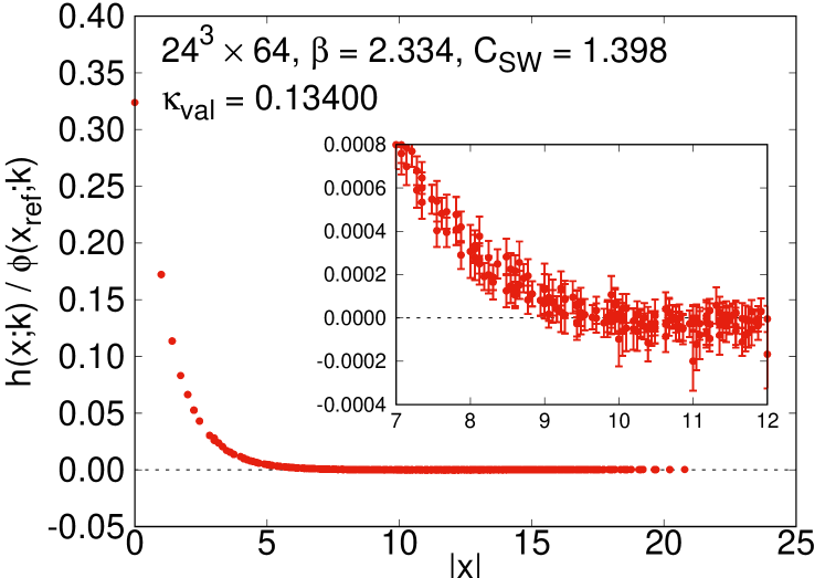
Figure 1: $h({\bf x};k)/\phi({\bf x}_{\rm ref};k)$ with ${\bf x}_{\rm ref}=(12,7,2)$ as a function of $x$. The inside panel shows the same data with an enlarged scale in $7\leq x\leq 12$.

Result: Figure 1 illustrates the result of $h({\bf x};k)/\phi({\bf x}_{\rm ref};k)$ as a function of $x$, which is calculated from a ratio of Eq. (9) to Eq. (8) at ${\bf x}_{\rm ref}=(12,7,2)$. In the figure and the following analyses, we choose $t=44$ for $C_{k}\phi({\bf x};k)$ in Eq. (8). We use $k^{2}$ determined from $E_{k}$ by a single exponential fit of $C_{\pi\pi}(t)=\sum_{\bf x}C_{\pi\pi}({\bf x},t)$ with a fit range of $12\leq t\leq 44$. The result of $k^{2}$ is presented in Table 1. In $x>10$, $h({\bf x};k)/\phi({\bf x}_{\rm ref};k)$ becomes consistent with zero in our statistics, suggesting the interaction range $R\sim 10<L/2=12$. Our calculation satisfies the sufficient condition to use Eq. (5). Our value of $R$ is consistent with that in Ref. Aoki et al. (2005).

$k^{2}$[GeV2]	$a_{0}/m_{\pi}(E_{k})$[GeV-2]	$a_{0}/m_{\pi}(H(k;k))$[GeV-2]
1.549(45)$\times 10^{-3}$	$-0.997(27)$	$-0.994(25)$

Table 1: Results for $k^{2}$, $a_{0}/m_{\pi}(E_{k})$ obtained by the finite volume method and $a_{0}/m_{\pi}(H(k;k))$ obtained by Eq. (17).

$H_{L}(k;k)$ is evaluated by performing the spatial summation in Eq. (10) with $p=k$. The result by all spatial summation agrees with that by up to $|{\bf x}|=10\sim R$, indicating the estimate of $R$ is valid.

We also examine whether $H_{L}(k;k)$ calculated on the lattice satisfies the condition of the finite volume method of Eq. (14). An indicator quantity $R({\bf x})$ is defined as

$$R({\bf x})=\frac{H_{L}(k;k)}{C_{k}\phi({\bf x};k)}G({\bf x};k)\xrightarrow[x>R]{}\frac{C_{00}H(k;k)}{v_{00}G({\bf x};k)}G({\bf x};k),$$ (16)

where we use Eqs. (11) and (12) in the arrow. $G({\bf x};k)$ is evaluated using the formula in Appendix B of Ref. Aoki et al. (2005). If Eq. (14) is satisfied, $R({\bf x})$ equals unity. The result of $R({\bf x})$ is plotted in Fig. 2. $R({\bf x})$ approaches unity in a large $x$ region, as expected. In $x>R\sim 10$, $R({\bf x})$ agrees with unity within 2 standard deviations.

$\tan\delta(k)$ is evaluated from $H_{L}(k;k)$ using the asymptotic form of $C_{k}\phi({\bf x},t)$ in Eq. (13) at a reference point ${\bf x}_{\rm ref}=(12,7,2)$. We choose ${\bf x}_{\rm ref}$, examining the size of the leading $l=4$ contribution in the dots terms by $Y_{40}(R_{A_{1}^{+}}[{\bf x}/x])j_{4}(kx)/(Y_{00}(R_{A_{1}^{+}}[{\bf x}/x])j_{0}(kx))$ at each position in $x>R$, where $Y_{lm}({\bf x}/x)$ are spherical harmonics. ${\bf x}_{\rm ref}$ is chosen such that $|Y_{40}(R_{A_{1}^{+}}[{\bf x}/x])j_{4}(kx)/(Y_{00}(R_{A_{1}^{+}}[{\bf x}/x])j_{0}(kx))|<10^{-6}$. $\tan\delta(k)$ is then given by

$$\tan\delta(k)=\frac{\sin(kx_{\rm ref})}{4\pi x_{\rm ref}C_{k}\phi({\bf x}_{\rm ref};k)/H_{L}(k;k)-\cos(kx_{\rm ref})},$$ (17)

where $H_{L}(k;k)/(C_{k}\phi({\bf x}_{\rm ref};k))=4\pi x_{\rm ref}\sin\delta(k)/\sin(kx_{\rm ref}+\delta(k))$. In the ratio $H_{L}(k;k)/(C_{k}\phi({\bf x}_{\rm ref};k))$, the overall factors of $H_{L}(k;k)$, $C_{00}e^{i\delta(k)}$, are canceled. We cannot determine the phase $e^{i\delta(k)}$ by this method. Correspondingly, the determination is impossible by the finite volume method.

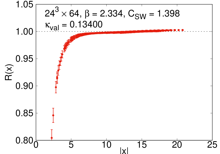
Figure 2: $R({\bf x})$ defined in Eq. (16) as a function of $x$. The dashed line expresses $R({\bf x})=1$.

The scattering length $a_{0}$ is obtained from $\tan\delta(k)$ as $a_{0}/m_{\pi}=\tan\delta(k)/(km_{\pi})$. We omit higher-order terms of $k^{2}$. $k^{2}$ is small enough in our calculation. Our result from Eq. (17) agrees with that from the finite volume method as shown in Table 1 and the value in Ref. Aoki et al. (2005). Those results are compared in Fig. 3. It is noted ambiguity from the choice of ${\bf x}_{\rm ref}$ is well below the statistical error. For example, we have $a_{0}/m_{\pi}=-1.001(27)$ with ${\bf x}_{\rm ref}=(10,4,4)$ and $a_{0}/m_{\pi}=-1.006(27)$ with ${\bf x}_{\rm ref}=(9,5,2)$.

As a check, the largest $l=4$ contribution in the dots terms of Eq. (13), which appears at ${\bf x}=(L/2,L/2,L/2)$, is also estimated. Using this position as ${\bf x}_{\rm ref}$ still leads to a similar result, $a_{0}/m_{\pi}=-0.967(25)$. It confirms the systematic error from the $l=4$ contribution is not significant compared to the statistical error.

The analysis using Eq. (16) and the comparison of $a_{0}/m_{\pi}$ conclude $H_{L}(k;k)$ calculated on the lattice satisfies Eq. (14) and gives $\delta(k)$ consistent with that by the finite volume method. The uncertainties in the two methods are also comparable. It should be emphasized that $H_{L}(k;k)$ is calculated using $\phi({\bf x};k)$ inside the interaction range, in contrast to the derivation of the finite volume method and the analysis of Ref. Aoki et al. (2005) using $\phi({\bf x};k)$ in $x>R$.

We also evaluate the half-off-shell amplitude $H(p;k)$ using Eq. (10). Figure 4 presents $H(p;k)$ as a function of $p^{2}$ normalized by its on-shell value as $\frac{H_{L}(p;k)}{H_{L}(k;k)}=\frac{H(p;k)}{H(k;k)}$. A clear signal of $H(p;k)$ is obtained. The result decreases as $p^{2}$ increases. In the figure, the inelastic threshold of the two-pion scattering is also plotted. It is smooth at the threshold, which may be due to the quenched approximation. While $H(p;k)$ cannot be directly compared with experiment, it might be an additional input to constrain parameters of effective models of hadron scatterings as a supplement to experimental data.

It is noted that the half-off-shell amplitude on the lattice itself depends on the choice of the operator. The dependence, however, is canceled in a ratio of $H_{L}(p;k)/H_{L}(k;k)$. We numerically confirmed the operator independence of $H_{L}(p;k)/H_{L}(k;k)=H(p;k)/H(k;k)$ by the use of wall sources, in addition to random sources. Both results agree within errors. If we employ a sink smearing of one of the pion operators for the BS wave function, an additional overall factor appears. This additional factor can be analytically erased Kawai et al. (2018).

We further attempt to extract information of the scattering from $H(p;k)$ with two assumptions. We assume that around $p^{2}=k^{2}$ the phase of $H(p;k)$ equals $e^{i\delta(k)}$, and $\partial(H(p;k)e^{-i\delta(k)})/\partial p^{2}\sim\partial(H(p;p)e^{-i\delta(p)})/\partial p^{2}$. Under the assumptions, the effective range expansion $k\cot\delta(k)=a_{0}^{-1}+rk^{2}+O(k^{4})$ leads to an estimate of the effective range $r$,

$$r=-\frac{2k^{2}H^{\prime}+\sin^{2}\delta(k)}{2k\sin\delta(k)\cos\delta(k)},$$ (18)

where $H^{\prime}$ is the slope of $H(p;k)/H(k;k)$ with respect to $p^{2}$ at $p^{2}=k^{2}$. Using our measured data, we estimate $r=-2.64(41)$ GeV^-1, which is not inconsistent with $r=-0.3(8.4)$ GeV^-1 using the data of $k\cot\delta(k)$ in Ref. Aoki et al. (2005).

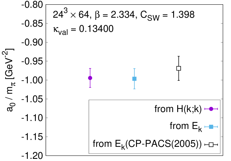
Figure 3: Comparison of scattering lengths $a_{0}/m_{\pi}$ from $H(k;k)$ with ${\bf x}_{\rm ref}=(12,7,2)$ (circle) and from the finite volume method (square), together with the result of Ref. Aoki et al. (2005) (open square).

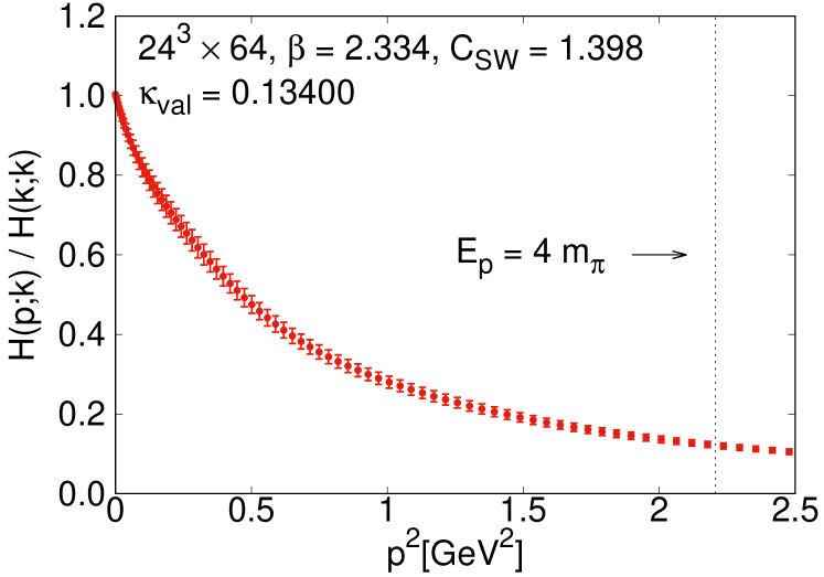
Figure 4: Half-off-shell amplitude $H(p;k)$ normalized by the on-shell value $H(k;k)$ as a function of $p^{2}$. The vertical dotted line denotes the threshold energy of the two-pion scattering.

Summary: We proposed a new method to calculate the scattering phase shift $\delta(k)$ from the on-shell scattering amplitude on the lattice $H_{L}(k;k)$ obtained with the BS wave function $\phi({\bf x};k)$ inside the interaction range by definition of quantum field theory. By a simulation of S-wave $I=2$ two-pion scattering in the center-of-mass frame, the consistency of our method with the finite volume method was examined. Our data of $R({\bf x})$ defined by Eq. (16) were found to satisfy the condition in the finite volume method of Eq. (14) in $x>R$. Our result of the scattering length $a_{0}/m_{\pi}$ from $H_{L}(k;k)$ agrees with the value from the finite volume method. The consistency concludes our method using information inside the interaction range can be an alternative to the finite volume method using data outside the interaction range.

We note issues of scaling violation. One is rotational symmetry breaking of $h({\bf x};k)$. It can be considered as a scaling violation of $H_{L}(k;k)$. The size of the rotational symmetry breaking in $H_{L}(k;k)$ is estimated by the difference between $H_{L}(k;k)$ with the minimum and maximum values of $h({\bf x};k)$ at each degenerate point of $|{\bf x}|$. The breaking effect is found to be 3%, close to our statistical error. Another is lattice artifacts of $h({\bf x};k)$ at small $|{\bf x}|$. The artifacts are expected to be significant, but suppressed in $H_{L}(k;k)$. It is clearly understood by the Jacobian factor $r^{2}$ of $H(p;k)$ in Eq. (5) in spherical coordinates. We noticed agreement between $a_{0}/m_{\pi}$ from $H(k;k)$ and that from the finite volume method in Fig. 3 indicates each method has a similar size of the scaling violation. Nevertheless, it is important future work to perform simulations at a different value of the lattice spacing for the investigation of the scaling violation.

We also evaluated the half-off-shell scattering amplitude $H_{L}(p;k)$ by lattice QCD. It might be a supplemental input to theoretical models of hadrons. We extracted the effective range from $H_{L}(p;k)$ with some assumptions. Although it was not inconsistent with the result from Ref. Aoki et al. (2005), our assumptions still need to be validated.

We remark it is essential to obtain the reduced BS wave function $h({\bf x};k)$ for the on-shell and half-off-shell amplitudes. $h({\bf x};k)$ is directly related to the amplitudes $H_{L}(p;k)$ in a simple form of Eq. (10). We may derive similar relations between the scattering amplitude and the reduced BS wave function in moving frames and scattering systems of more than two particles.

Acknowledgments: We thank N. Ishizuka and Y. Kuramashi for their careful reading of the manuscript and useful comments. Our simulation was performed on COMA under Interdisciplinary Computational Science Program of Center for Computational Sciences, University of Tsukuba. This work is in part based on the Bridge++ code Bri . This work is supported in part by JSPS KAKENHI Grants No. 15K05068 and No. 16H06002.

References

- Lüscher (1986) M. Lüscher, Commun. Math. Phys. 105, 153 (1986).
- Lüscher (1991) M. Lüscher, Nucl. Phys. B354, 531 (1991).
- Lin et al. (2001) C. J. D. Lin, G. Martinelli, C. T. Sachrajda, and M. Testa, Nucl. Phys. B619, 467 (2001), arXiv:hep-lat/0104006 [hep-lat] .
- Aoki et al. (2005) S. Aoki, M. Fukugita, K.-I. Ishikawa, N. Ishizuka, Y. Iwasaki, T. Kaneko, Y. Kuramashi, M. Okawa, A. Ukawa, T. Yamazaki, and T. Yoshié (CP-PACS Collaboration), Phys. Rev. D71, 094504 (2005), hep-lat/0503025 .
- Yamazaki and Kuramashi (2017) T. Yamazaki and Y. Kuramashi, (2017), to appear in Phys. Rev. D, arXiv:1709.09779 [hep-lat] .
- Aoki et al. (2010) S. Aoki, T. Hatsuda, and N. Ishii, Prog.Theor.Phys. 123, 89 (2010), arXiv:0909.5585 [hep-lat] .
- Lellouch and Luscher (2001) L. Lellouch and M. Luscher, Commun. Math. Phys. 219, 31 (2001), arXiv:hep-lat/0003023 [hep-lat] .
- Ali Khan et al. (2002) A. Ali Khan, S. Aoki, G. Boyd, R. Burkhalter, S. Ejiri, M. Fukugita, S. Hashimoto, N. Ishizuka, Y. Iwasaki, K. Kanaya, T. Kaneko, Y. Kuramashi, T. Manke, K. Nagai, M. Okawa, H. P. Shanahan, A. Ukawa, and T. Yoshié (CP-PACS Collaboration), Phys. Rev. D65, 054505 (2002), [Erratum: Phys. Rev.D67,059901(2003)], arXiv:hep-lat/0105015 .
- (9) Y. Iwasaki, Report No. UTHEP-118 (Dec. 1983), arXiv:1111.7054 [hep-lat] .
- Iwasaki (1985) Y. Iwasaki, Nucl. Phys. B258, 141 (1985).
- Sheikholeslami and Wohlert (1985) B. Sheikholeslami and R. Wohlert, Nucl. Phys. B259, 572 (1985).
- Kawai et al. (2018) D. Kawai, S. Aoki, T. Doi, Y. Ikeda, T. Inoue, T. Iritani, N. Ishii, T. Miyamoto, H. Nemura, and K. Sasaki (HAL QCD), PTEP 2018, 043B04 (2018), arXiv:1711.01883 [hep-lat] .
- (13) See http://bridge.kek.jp/Lattice-code/ .