Nanoscopy of pairs of atoms by fluorescence in a magnetic field

Abstract

Spontaneous emission spectra of two initially excited closely spaced identical atoms are very sensitive to the strength and the direction of the applied magnetic field. We consider the relevant schemes that ensure the determination of the mutual spatial orientation of the atoms and the distance between them by entirely optical means. A corresponding theoretical description is given accounting for the dipole-dipole interaction between the two atoms in the presence of a magnetic field and for polarizations of the quantum field interacting with magnetic sublevels of the two-atom system.

I INTRODUCTION

Ultrahigh spatial resolution at the distances short compared to optical wavelength is a challenging spectroscopic problem. Various approaches to solution of this problem have been suggested, and some of them have been realized in the experiment. The following ideas can be mentioned: (i) the photoelectron (photoion) microscopy LETOKHOV1 ; LETOKHOV2 ; LETOKHOV3 being a development of the Müller emission microscope MULLER ; (ii) the transport of the molecule excitation between a nanosize needle tip and bulk via the fluorescence resonance energy transfer (FRET) KOPELMAN ; (iii) FRET scanning near-field optical microscopy SL ; SEKATSKII ; (iv) combinations of the optical excitation with nano-resolution of the atomic force microscope or scanning tunnel microscope LAPSHIN ; (v) the transport of a laser excited atom through a nanohole in a metal screen BALYKIN .

A system of two closely spaced identical atoms (quantum dots, vacancy centers, organic molecules in solid solutions, etc.) is the simplest model where a determination of, at least, two parameters might be desirable. These parameters are the distance between the atoms and the direction of their vector separation in the space. In this paper, we consider a method for their estimation by only optical means, without any nano-tools like needles, tips, or holes. (For a possible solution of this task in 2D see, e.g., Ref. SUN ).

A system of two identical atoms with the ground states $|g_{1,2}\rangle$ and the excited states $|e_{1,2}\rangle$ is an example exhibiting the effects of Dicke super- and subradiance DICKE . The two excited states of this system are $|{\mathcal{Q}}_{1}\rangle=|e_{1}g_{2}\rangle$ and $|{\mathcal{Q}}_{2}\rangle=|g_{1}e_{2}\rangle$. The dipole-dipole interaction between the states $|{\mathcal{Q}}_{1}\rangle$ and $|{\mathcal{Q}}_{2}\rangle$ leads to their superpositions producing two entangled eigenstates, symmetric and antisymmetric (see, e.g., Refs. FICEK ; BGZ ). While the symmetric state $|{\mathcal{Q}}_{s}\rangle={\frac{1}{{\sqrt{2}}}}\left(|{\mathcal{Q}}_{1}\rangle+|{\mathcal{Q}}_{2}\rangle\right)$ is superradiant, decaying twice faster than the one-atom state $|e\rangle$, the antisymmetric state $|{\mathcal{Q}}_{a}\rangle={\frac{1}{{\sqrt{2}}}}\left(|{\mathcal{Q}}_{1}\rangle-|{\mathcal{Q}}_{2}\rangle\right)$ is subradiant, decaying slowly by the parameter $(r/\lambda_{eg})^{2}$ if the distance $r$ between the atoms is smaller then the wavelength of the $|e\rangle\rightarrow|g\rangle$ transition. The theory of this system (with an emphasis on superradiance) was studied in a number of works (see, e.g., Refs. LEMBERG ; MILLONI ; WANG , and the review FICEK ). An interesting effect of the exchange between symmetric and antisymmetric states due to the spatial variation of the applied laser pulse at the positions of the atoms was discovered in Ref. DAS . As for the subradiant states, they attracted a special attention because of their property of a relatively slow spontaneous decay and, hence, a potentiality of keeping quantum information for a long time.

A prominent effect of subradiance can be achieved in the one-dimensional (1D) case ML ; RY (using, e.g., a single-mode waveguide or a photon crystal) where two spatially separated atoms are placed at a distance of the whole number of the half-wavelengths of the optical transition. Several methods were suggested to produce subradiant states. E.g., in the mentioned 1D case, the subradiant state is produced with a probability of $\approx 1/2$, when, at the initial moment of time, one of the atoms is excited. More complicated configuration in a 1D waveguide have been also considered (see, e.g. Bar-⁠2017 ). However, this schemes can be realized only for spatially separated atoms. For closely spaced atoms in 3D, two schemes of control of subradiance can be mentioned ZADKOV ; JETPLETT , the both showing reasonable fidelity. An interesting scheme for producing the single-photon subradiant state in an ensemble of many atoms was recently considered by Scully SCULLY1 . Protection of this state was discussed in Ref. SCULLY2 . As for the experiment on subradiance, certain evidences for modification of the decay rate were received, e.g., in Ref. PAVOLINI for large atomic ensemble, and in Ref. BREWER for a system of two trapped ions. Subradiance was also observed very recently for a cloud of cold atoms GUERIN . The contribution of this effect was small, but detectable as a narrow spectrum of fluorescence gated at times much longer than the time of single-atom decay. In connection with this experimental work, a recent theoretical paper HKOR should be mentioned where the property of subradiance in atomic ensembles has been argued to be more general than this is usually assumed.

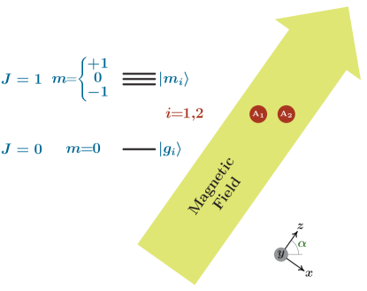
Figure 1: Our model. Two identical atoms A₁ and A₂ are located in the $xz$ plane. The angular momenta of their ground state $|g\rangle$ and excited state $|e\rangle$ are, respectively, $J_{g}=0$ and $J_{e}=1$. Magnetic field is directed along the $z$ axis. The line connecting the atoms is directed at a certain angle $\alpha$ to the z axis. This leads to splitting of the excited state into the triplet of states with the $J$-projections $m=0,\pm 1$ on the $z$ axis. (In our consideration, the main results refer to the magic angle $\alpha=\alpha_{\textrm{mag}}=\arccos(1/{\sqrt{3}})\approx 54.7^{o}$.)

In this paper we consider the fluorescence spectra of two closely spaced identical atoms in a magnetic field. We use the remarkable fact that, being directed at the magic angle $\alpha\approx\arccos(1/\sqrt{3})\approx 54.7^{\textrm{o}}$ relative to the direction from one atom to another (see Fig. 1), a sufficiently strong magnetic field suppresses the dipole-dipole excitation transfer from one atom to the other one CONTROL . This makes the fluorescence spectrum following the excitation of the both atoms be very sensitive to small deflections from the magic-angle configuration (see Fig. 2). This observation helps one to determine the direction of the vector separation by a series of manipulations with a magnetic field. To demonstrate the relevant procedure, first, in Sec. II, we describe the model, write down the Hamiltonian of our system, and derive properties of its eigenstates. Then, in Sec. III, we consider general theory of interaction of the two-atom system with the electromagnetic field. Next, in Sec. IV, we consider its consequences concerning fluorescence spectra in a magnetic field of (i) singly-excited entangled states (Sec. IV.1), and (ii) doubly-excite states Sec. IV.2) where, in particular, it is shown (Sec. IV.2.2) how the distance between the atoms can be estimated from the probability of the gated fluorescence from the subradiant state only. Finally, in Sec. V, we show how the full nanoscopy of a pair of atoms can be completed, i.e. in addition to the distance between the atoms (Sec. IV.2.2), the direction of the vector separation from one atom to another can be determined. The latter is achieved using the above announced sensitivity (see Fig. 2 supported by calculations of Sec. IV.2.3) of the fluorescence spectra to the direction of the magnetic field.

The calculation details are presented in the Appendices.

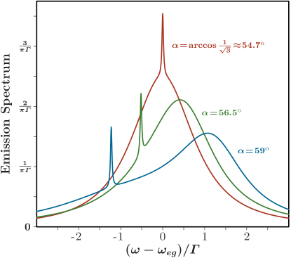
Figure 2: An example of emission spectra of a two-atom system in a strong magnetic field H at different values of the angle $\alpha$ (see Fig. 1). Initially (at $t=0$) the both atoms are excited to the state $|e\rangle$ with $m=0$. The rate of spontaneous transition $|e\rangle\rightarrow|g\rangle$ is $\varGamma$. The transition frequency is $\omega_{eg}$ and the corresponding wave vector is $k_{0}$. For this example, the atoms are located so that $k_{0}r=0.5$. For calculation of these spectra, see Sec. IV.2.3.

II Description of the two-atom system

The system of two closely located identical atoms in an external magnetic field $\bf{H}$ directed along the $z$-axis is shown in Fig. 1. The vector $\bf{r}$ connecting the positions of two atoms meets at an angle $\alpha$ with the field $\bf{H}$; below we choose the $x$ and $y$ coordinate axes such that

$${\bf{r}}=(r_{x},r_{y},r_{z})=r(\sin{\alpha},0,\cos{\alpha})\;.$$ (1)

It is assumed that the ground state $|g\rangle$ of the atom is non-degenerate and corresponds to the angular momentum $J=0$, while the excited state $|e\rangle$ of our interest is a triplet of states $|e^{(m)}\rangle$ (just $|m\rangle$ below for shortness) corresponding to the momentum $J=1$ with projections $m=0,\pm 1$ on the quantization axis $z$. In a zero magnetic field this triplet is degenerate and its energy (counted from the ground atomic state) is $\omega_{eg}$. Nonzero components of the dipole moment operator $\widehat{{\bf{d}}}$ between the states $|g\rangle$ and $|m\rangle$ are (see Appendix A) given by

$$\langle m=0|\hat{d}_{z}|g\rangle\equiv d_{0}\;,\,\,\,\,\langle m=\pm 1|\hat{d}_{\pm}|g\rangle=\sqrt{2}d_{0}\;,$$ (2)

where $\hat{d}_{\pm}\equiv\hat{d}_{x}\pm i\hat{d}_{y}$ are the circular components.

The reduced Hilbert space of the two-atom system can be described by the following basis: $\left\{|g,g\rangle;|m,g\rangle;|g,m\rangle,|m,m^{\prime}\rangle\right\}$, where the two-atom state $|a,b\rangle=|a\rangle_{1}\otimes|b\rangle_{2}$ is a direct product of the states of the first and the second atoms. The first state in curly brackets corresponds to the ground state, the second and third ones—to singly excited states, and the forth one to a doubly excited state of the two-atom system. In this paper we consider only symmetric doubly-excited states of the form $|m,m\rangle$ that can be created by an optical $\pi$-pulse of a certain polarization, linear or circular. To account for the symmetry of the two-atom system with one excitation, it is convenient to introduce new basis of symmetric and antisymmetric states:

$$|s_{m}\rangle=\frac{1}{\sqrt{2}}(|m,g\rangle+|g,m\rangle)\;,$$ (3)

$$|a_{m}\rangle=\frac{1}{\sqrt{2}}(|m,g\rangle-|g,m\rangle)\;.$$ (4)

The Hamiltonian $\widehat{H}$ of the two atom system can be represented as a sum $\widehat{H}^{(1)}+\widehat{H}^{(2)}$ of two Hamiltonians acting in the subspaces with one and two excitations, respectively. An important constituent of the Hamiltonian $\widehat{H}$ of closely located atoms is the operator $\widehat{U}$ of the dipole-dipole interatomic interaction:

$$\widehat{U}=\frac{\left(\widehat{\bf{d}}_{1}\!\cdot\!\widehat{\bf{d}}_{2}\right)}{r^{3}}-3\frac{\left(\widehat{\bf{d}}_{1}\!\cdot\!\bf{r}\right)\left(\widehat{\bf{d}}_{2}\!\cdot\!\bf{r}\right)}{r^{5}}\;,$$ (5)

where $\widehat{\bf{d}}_{1(2)}$ is the dipole moment operator of the first (second) atom. This interaction is not important for doubly excited states: the induced coupling between doubly excited and ground states results only in a parametrically weak ($\sim d^{2}_{0}/\hbar r^{3}\omega_{eg}\ll 1$) renormalization of state parameters that will be neglected below. So, the Hamiltonian $\widehat{H}^{(2)}$ in the subspace of our interest can be represented as

$$\widehat{H}^{(2)}=\sum_{m}(2\hbar\omega_{eg}+2m\varOmega_{H})|m,m\rangle\langle m.m|\;,$$ (6)

where $\varOmega_{H}=\mu_{\textrm{B}}gH$ describes the Zeeman splitting of levels in the magnetic field ($\mu_{\textrm{B}}$ is the Bohr magneton, and g is the Landé factor).

The interaction $\widehat{U}$ is mixing the states with different projections $m$ in the subspace with one excitation. As $\widehat{U}$ does not mix states with different symmetries, the matrix of the Hamiltonian $\widehat{H}^{(1)}$ in the basis (3)–(4) is split into two parts, $\widehat{H}^{(1)}_{s}$ and $\widehat{H}^{(1)}_{a}$:

$$\widehat{H}^{(1)}_{s}=\hbar\omega_{eg}\widehat{\mathbb{I}}+U_{r}\begin{pmatrix}-\frac{\varOmega_{H}}{U_{r}}\!+\!(1\!-\!\frac{3}{2}\sin^{2}\alpha)&-\frac{3\sqrt{2}}{4}\sin 2\alpha&-\frac{3}{2}\sin^{2}\alpha\\ -\frac{3\sqrt{2}}{4}\sin 2\alpha&(1\!-\!3\cos^{2}\alpha)&-\frac{3\sqrt{2}}{4}\sin 2\alpha\\ -\frac{3}{2}\sin^{2}\alpha&-\frac{3\sqrt{2}}{4}\sin 2\alpha&\frac{\varOmega_{H}}{U_{r}}\!+\!(1\!-\!\frac{3}{2}\sin^{2}\alpha)\end{pmatrix}\;,$$ (7)

$$\widehat{H}^{(1)}_{a}=\hbar\omega_{eg}\widehat{\mathbb{I}}+U_{r}\begin{pmatrix}-\frac{\varOmega_{H}}{U_{r}}\!-\!(1\!-\!\frac{3}{2}\sin^{2}\alpha)&\frac{3\sqrt{2}}{4}\sin 2\alpha&\frac{3}{2}\sin^{2}\alpha\\ \frac{3\sqrt{2}}{4}\sin 2\alpha&-(1\!-\!3\cos^{2}\alpha)&\frac{3\sqrt{2}}{4}\sin 2\alpha\\ \frac{3}{2}\sin^{2}\alpha&\frac{3\sqrt{2}}{4}\sin 2\alpha&\frac{\varOmega_{H}}{U_{r}}\!-\!(1\!-\!\frac{3}{2}\sin^{2}\alpha)\end{pmatrix}\;,$$ (8)

where the rows and columns are enumerated in the order $m=-1,0,1$, $\widehat{\mathbb{I}}$ is the unit matrix in the space spanned by (3)–(4), $U_{r}=d_{0}^{2}/r^{3}$, and an explicit form of angular parts of the wavefunctions corresponding to $|g\rangle$ and $|m\rangle$ is given in Appendix A.

Eqs. (7)–(8) are simplified for the above introduced magic angle (see Fig. 1), when the diagonal part of the dipole-dipole interaction vanishes, and have next form

$$\widehat{H}^{(1)}_{s}=\hbar\omega_{eg}\widehat{\mathbb{I}}+U_{r}\begin{pmatrix}-\frac{\varOmega_{H}}{U_{r}}&-1&-1\\ -1&0&-1\\ -1&-1&\frac{\varOmega_{H}}{U_{r}}\end{pmatrix}\,,$$ (9)

$$\widehat{H}^{(1)}_{a}=\hbar\omega_{eg}\widehat{\mathbb{I}}+U_{r}\begin{pmatrix}-\frac{\varOmega_{H}}{U_{r}}&1&1\\ 1&0&1\\ 1&1&\frac{\varOmega_{H}}{U_{r}}\end{pmatrix}\,.$$ (10)

The eigenenergies of the two Hamiltonians are determined by the characteristic equations:

$$\left(E^{s(a)}\right)^{3}-\left(\varOmega_{H}^{2}+3U_{r}^{2}\right)E^{s(a)}\pm 2U_{r}^{3}=0\;,$$ (11)

where $E^{s(a)}$ are counted from the atomic transition frequency $\omega_{eg}$. In the absence of the magnetic field, the solutions $E^{s(a)}_{j}$ of the characteristic equations (it is convenient to numerate them by $j=-1,0,1$ in the ascending order) are:

$$E^{s}_{-1}\!=\!-2U_{r},\;E^{s}_{0(1)}\!=\!U_{r};\;E^{a}_{-1(0)}\!=\!-U_{r},\;E^{a}_{+1}\!=\!2U_{r}\;.$$ (12)

In the opposite case of a strong magnetic field, the role of the dipole-dipole interaction is small, the eigenstates only slightly differ from $|s_{m}\rangle$ and $|a_{m}\rangle$, and eigenenergies are given by

$$E^{\nu}_{\pm 1} \approx m\left(\varOmega_{H}+\frac{3U_{r}^{2}}{2\varOmega_{H}}\right)-\frac{\nu U_{r}^{3}}{\varOmega_{H}^{2}}\;,$$ (13)

$$E^{\nu}_{0} \approx\frac{2\nu U_{r}^{3}}{\varOmega^{2}_{H}}\;,$$ (14)

where $\nu=\pm 1$ for the symmetric and antisymmetric states, respectively. For an arbitrary magnitude of the magnetic field (and $\alpha=\alpha_{\textrm{mag}}$), the eigenenergies are presented in Fig. 3.

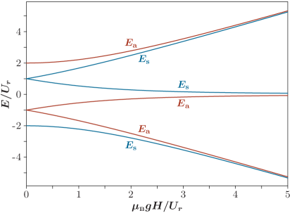
Figure 3: Energies of eigenstates of a system of two atoms as functions of the magnetic field ${\bf{H}}$ applied at the magic angle as shown in Fig. 1.

For further purposes we also present the expression for the energy $E^{\nu}_{0}$ for the case of an arbitrary angle $\alpha$:

$$E^{\nu}_{0}\approx\nu U_{r}\left[1-3\cos^{2}{\alpha}+{\frac{27U_{r}^{2}}{\varOmega_{H}^{2}}}\sin^{2}{\alpha}\cos^{4}{\alpha}\right]\;.$$ (15)

In a close vicinity of the magic angle this expression takes the form:

$$E^{\nu}_{0}\approx 2\nu U_{r}\left[{\sqrt{2}}(\alpha-\alpha_{\textrm{mag}})+\frac{U_{r}^{2}}{\varOmega_{H}^{2}}\right]\;.$$ (16)

As seen from Eqs. (14)–(16), the detuning of $E^{\nu}_{0}$ from zero decreases dramatically when $\alpha\rightarrow\alpha_{\textrm{mag}}$. The same is for the splitting between $E^{s}_{\pm 1}$ and $E^{a}_{\pm 1}$.

Eigenvectors $|\psi_{j}^{s}\rangle$ and $|\psi_{j}^{a}\rangle$ (numerated by $j=-1,0,1$) of the matrices $\widehat{H}^{(1)}_{s}$ and $\widehat{H}^{(1)}_{a}$ form bases connected with $\left\{|s_{m}\rangle\right\}$ and $\left\{|a_{m}\rangle\right\}$ by a unitary matrix $\widehat{C}^{\nu}$

$$|\nu_{m}\rangle=\sum_{j}C_{mj}^{\nu}|\psi_{j}^{\nu}\rangle\;,$$ (17)

where $\nu=s,a$. These eigenvectors can be expressed in terms of the elements of the matrices (9)–(10), and the corresponding eigenenergies $E^{\nu}_{j}$ ($\nu=s,a$; $j=-1,0,1$) defined by Eq. (11). In the basis $|\nu_{m}\rangle$ ($m=-1,0,1$) defined by Eqs. (3)–(4) they are

$$|\psi_{j}^{\nu}\rangle=q^{\nu}_{j}\left(\begin{array}[]{c}\frac{E^{\nu}_{j}\mp U_{r}}{\varOmega_{H}+E^{\nu}_{j}\mp U_{r}}\\ 1\\ -\frac{E^{\nu}_{j}\mp U_{r}}{\varOmega_{H}-E^{\nu}_{j}\pm U_{r}}\\ \end{array}\right)\equiv\sum_{m}Q^{\nu}_{jm}|\nu_{m}\rangle\;,$$ (21)

where the upper (lower) sign refers to the symmetric (antisymmetric) state $s$ ($a$), and

$$q^{\nu}_{j}\!=\!\left[\left(\frac{E^{\nu}_{j}\mp U_{r}}{\varOmega_{H}\!+\!E^{\nu}_{j}\mp U_{r}}\right)^{2}\!+\!1\!\right.\left.+\!\left(\frac{E^{\nu}_{j}\mp U_{r}}{\varOmega_{H}\!-\!E^{\nu}_{j}\pm\!U_{r}\!}\right)^{2}\right]^{-1/2}\,.$$ (22)

The matrix $\widehat{C}^{\nu}$ is connected with $\widehat{Q}^{\nu}$ as $C^{\nu}_{mj}=Q^{\nu}_{jm}$.

In the next section we develop a convenient description of the interaction of the two-atom system with the electromagnetic field.

III Interaction with the electromagnetic field

The Hamiltonian of the two-atom system interacting with the electromagnetic field has the form:

$$\widehat{\mathcal{H}}=\widehat{H}+\widehat{H}_{\textrm{ph}}+\widehat{H}_{\textrm{int}}\;,$$ (23)

$$\widehat{H}_{\textrm{ph}}=\sum_{{\bf k}\lambda}\hbar\omega_{k}a_{{\bf k}\lambda}^{{\dagger}}a_{{\bf k}\lambda}\;,$$ (24)

where the two-atom Hamiltonian $\widehat{H}$ has been defined in the previous section, and $\widehat{H}_{\textrm{ph}}$ corresponds to free photons, $\omega_{k}$ and $\bf{k}$ being the photon frequency and wave vector, so $a_{{\bf k}\lambda}^{{\dagger}}$ ($a_{{\bf k}\lambda}$) is a photon creation (annihilation) operator with $\lambda=1,2$ meaning the two linear polarizations. The interaction Hamiltonian $\widehat{H}_{\textrm{int}}$ can be split into two parts $\widehat{H}^{(1)}_{\textrm{int}}+\widehat{H}^{(2)}_{\textrm{int}}$ that correspond to optical transitions between the ground and a singly excited state of the two-atom system and between the singly and a doubly excited states, respectively.

In the rotating wave approximation (RWA) the first part, $\widehat{H}^{(1)}_{\textrm{int}}$, can be represented as

$$\widehat{H}^{(1)}_{\textrm{int}}=-\sum_{{\bf{k}},\lambda,m}\left\{g_{\bf{k}\lambda}^{m,g}\left[|m,g\rangle\langle g,g|e^{-i\frac{\bf{k}\bf{r}}{2}}\right.\right.$$

$$\left.\left.+|g,m\rangle\langle g,g|e^{i\frac{\bf{k}\bf{r}}{2}}\right]a_{\bf{k}\lambda}+{\mathrm{H.c.}}\right\}\;.$$ (25)

Here H.c. means Hermitian conjugate, the first and the second terms in the square bracket correspond, respectively, to the optical excitation of only the first atom (located at $-{\bf{r}}/2$) and of only the second atom (located at ${\bf{r}}/2$), the matrix element of the dipole transition is given by

$$g_{{\bf{k}}\lambda}^{m,g}=\sqrt{\frac{2\pi\hbar\omega_{{\bf k}}}{V}}\langle m|{\hat{{\bf{d}}}}|g\rangle{\bf{e}}_{{\bf{k}}\lambda}\,,$$ (26)

where $V$ is the quantization volume, $\bf{e}_{{\bf k}\lambda}$ is the polarization vector. Below we will replace the photon frequency $\omega_{{\bf k}}$ in Eq. (26) by the resonance transition frequency $\omega_{eg}$. A similar expression can be written for the part $\widehat{H}^{(2)}_{\textrm{int}}$ with the only difference that the transitions take place between the states $|m,g\rangle$ (or $|g,m\rangle$) and $|m,m^{\prime}\rangle$ ($|m^{\prime},m\rangle$). Restricting our consideration to only symmetric doubly excited states $|m,m\rangle$, we have

$$\widehat{H}^{(2)}_{\textrm{int}}=-\sum_{\bf{k},\lambda,m}\left\{g_{\bf{k}\lambda}^{m,g}|m,m\rangle\left[\langle m,g|e^{i\frac{\bf{k}\bf{r}}{2}}\right.\right.$$

$$\left.\left.+\langle g,m|e^{-i\frac{\bf{k}\bf{r}}{2}}\right]a_{\bf{k}\lambda}+{\mathrm{H.c.}}\right\}\,.$$ (27)

The choice of the polarization vectors and explicit expressions for the matrix element given by Eq. (26) are described in the Appendix A. Here we only briefly discuss the main steps of the further analysis.

(i) We express singly excited states of the two-atom system in terms of the symmetric and antisymmetric combinations (3) and (4), and, finally, in terms of exact states $\left\{\right|\psi^{\nu}_{j}\rangle;j=-1,0,1\}$ [see Eq. (17)] of a definite symmetry ($\nu=s,a$).

(ii) To simplify calculations we use the symmetry of the system and introduce new (“symmetric” and “antisymmetric”) photon operators:

$$b_{1s}(\bf{k})=\frac{1}{\sqrt{2}}[a_{\bf{k}1}-a_{-\bf{k}1}],$$ (28)

$$b_{1a}(\bf{k})=\frac{1}{\sqrt{2}}[a_{\bf{k}1}+a_{-\bf{k}1}],$$ (29)

$$b_{2s}(\bf{k})=\frac{1}{\sqrt{2}}[a_{\bf{k}2}+a_{-\bf{k}2}],$$ (30)

$$b_{2a}(\bf{k})=\frac{1}{\sqrt{2}}[a_{\bf{k}2}-a_{-\bf{k}2}],\,.$$ (31)

To avoid double counting we restrict the photon wave vector $\bf{k}$ to the upper hemisphere $k_{z}\geqslant 0$. Then the above set of new operators is complete, and obeys the usual boson commutation relations:

$$[b_{1s}({\bf{k}}),b^{\dagger}_{1s}({\bf{k}}^{\prime})]=\delta_{{\bf{k}},{\bf{k}}^{\prime}}=[b_{2s}({\bf{k}}),b^{\dagger}_{2s}({\bf{k}}^{\prime})]\;,$$ (32)

$$[b_{1s}({\bf{k}}),b^{\dagger}_{1a}({\bf{k}}^{\prime})]=0\;.$$ (33)

Now, the free photon Hamiltonian is

$$\widehat{H}_{\textrm{ph}}=\sum\nolimits^{\prime}_{{\bf k};\lambda=1,2;\nu=s,a}\hbar\omega_{k}b_{\lambda\nu}^{\dagger}({\bf{k}})b_{\lambda\nu}({\bf{k}})\;,$$ (34)

where the prime sign denotes the summation over the upper hemisphere of $\bf{k}$. The interaction part becomes

$$\widehat{H}^{(1)}_{\textrm{int}}=-2\sideset{}{{}^{\prime}}{\sum}_{{\bf{k}}^{\prime}\!,\lambda,j}\left\{g_{{\bf{k}}^{\prime}\!\lambda}^{m,g}\left[\cos\left({\frac{{\bf{kr}}}{2}}\right)C_{mj}^{s}|\psi_{j}^{s}\rangle b_{\lambda s}({\bf{k}}^{\prime})\right.\right.\\ \left.\left.-i\sin\left({\frac{{\bf{kr}}}{2}}\right)C_{mj}^{a}|\psi_{j}^{a}\rangle b_{\lambda a}({\bf{k}}^{\prime})\right]\langle g,g|+{\mathrm{H.c.}}\right\}\,,$$ (35)

$$\widehat{H}^{(2)}_{\textrm{int}}=-2\sideset{}{{}^{\prime}}{\sum}_{{\bf{k}}^{\prime}\!,\lambda,j}\left\{g_{{\bf{k}}^{\prime}\!\lambda}^{m,g}|m,m\rangle\left[\cos\left({\frac{{\bf{kr}}}{2}}\right)C_{mj}^{s}|\psi_{j}^{s}\rangle b_{\lambda s}({\bf{k}}^{\prime})\right.\right.\\ \left.\left.+i\sin\left({\frac{{\bf{kr}}}{2}}\right)C_{mj}^{a}|\psi_{j}^{a}\rangle b_{\lambda a}({\bf{k}}^{\prime})\right]+{\mathrm{H.c.}}\right\}\,,$$ (36)

where the matrices $C_{mj}^{\nu}$ ($\nu=s,a$) are defined by Eq. (17).

Eqs. (34)–(36) explicitly demonstrate the important properties of the system: (i) the symmetric and antisymmetric singly excited states decay to the ground states independently of each other; the decay is caused by the interaction with only symmetric or antisymmetric photon continua, respectively; (ii) the decay of a doubly excited state (of the form $|m,m\rangle$) to a singly excited one can go both via the symmetric and antisymmetric channels. The decay scheme is shown in Fig. 4.

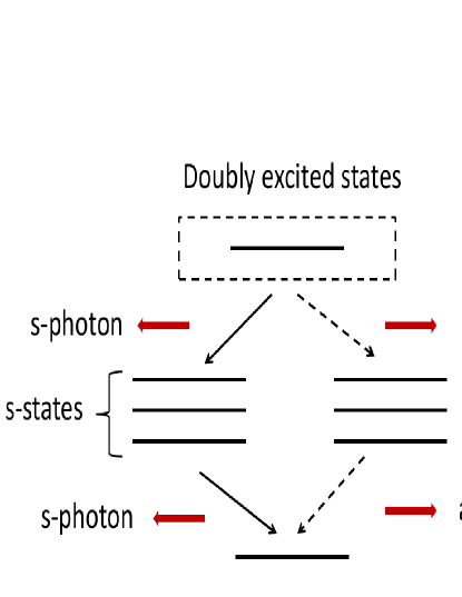
Figure 4: Scheme of the spontaneous decay of the doubly excited states of a system of two atoms. There are two ways of the decay whose branching ratio depends on the distance between the atoms.

In the case of interest, when the interatomic separation is small ($kr\ll 1$), the matrix elements of the symmetric and antisymmetric channels enter Eqs. (III) and (III) with rather different weights: the symmetric one $\propto\cos\left(\frac{\bf{kr}}{2}\right)\approx 1$, while the antisymmetric one $\propto\sin\left(\frac{\bf{kr}}{2}\right)\approx{\bf{kr}}/2\ll 1$. This means that the ratio of the decay rates via corresponding channels scales as $\varGamma_{a}/\varGamma_{s}\propto(k_{0}r)^{2}\ll 1$, where $k_{0}$ is the wave vector that corresponds to the transition frequency $\omega_{eg}$.

Some implementations of the developed formalism are given in the subsequent sections.

IV Fluorescence spectra of the two-atom system

IV.1 Decay rate of a singly excited system

Consider the two-atom system originally (at the time $t=0$) prepared in one of the eigenstates $\psi^{\nu}_{j}$ of a definite symmetry $\nu=s,a$. The time evolution of the atom-photon system is described by the wave function

$$|\varPsi(t)\rangle=A_{j}^{\nu}(t)|\psi^{\nu}_{j}\rangle\otimes|{\textsl{vac}}\rangle\\ +\sideset{}{{}^{\prime}}{\sum}_{{\bf{k}},\lambda}B^{\nu}_{{\bf{k}}\lambda}(t)|g,g\rangle\otimes b_{\lambda\nu}^{\dagger}(\bf{k})|{\textsl{vac}}\rangle\,$$ (37)

determined by the Schrödinger equation with the interaction Hamiltonian $\widehat{H}^{(1)}_{\textrm{int}}$ (35) and the initial condition $A_{j}^{\nu}(0)=1$, $B^{\nu}_{{\bf{k}}\lambda}(0)=0$; the state $|{\textsl{vac}}\rangle$ is the vacuum state of the electromagnetic field (no photons). Assuming that the interval between energy levels of the same symmetry is much greater than the level’s widths we have neglected in Eq. (37) an admixture of other excited states in the course of decay. As the decay of the atomic state of a given symmetry $\nu$ involves only photons of the same symmetry, the problem is similar to the usual one-atom decay problem and here we write down the calculated decay constants (referring to Appendix A1 for technical details). The decay constant for the symmetric singly excited state is

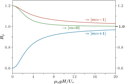
Figure 5: Magnetic field dependence of the decay rate coefficients $R_{j}$ defined by Eqs. (41)–(42). The field ${\bf{H}}$ is directed at the angle $\alpha=\alpha_{\textrm{mag}}$ relative to the vector separation ${\bf{r}}$ between the atoms. Arrows indicate to which $|m\rangle$-state a given $j$-eigenstate transforms as ${\bf{H}}$ increases.

$$\varGamma_{s}\approx 2\varGamma\,,$$ (38)

where $\varGamma$ is the decay rate for a single atom

$$\varGamma=\frac{4}{3}\frac{\omega^{3}_{eg}d^{2}_{0}}{\hbar c^{3}}\;.$$ (39)

We see that decay rate of the symmetric states demonstrates the expected superradiance property and is almost non-sensitive to the magnetic field. On the contrary, the decay rate of antisymmetric states $\varGamma_{a}$ is strongly suppressed (subradiant). In the case of a strong magnetic field ($\varOmega_{H}\gg U_{r}$) and $\alpha=\alpha_{\textrm{mag}}$, the decay rate of any singly excited antisymmetric state is given by

$$\varGamma_{a}\approx{\frac{1}{6}}(k_{0}r)^{2}\varGamma\;$$ (40)

(see Ref. MAK and Sec. 1 of Appendix A). For the intermediate field magnitudes the decay rate of a state $|\psi^{a}_{j}\rangle$ takes the form:

$$\varGamma_{aj}=R_{j}\varGamma_{a}\;,$$ (41)

where the numerical coefficient $R_{j}$ is a combination

$$R_{j}=1-\frac{1}{5}\sum\nolimits_{m,m^{\prime}\neq m}C^{a}_{mj}(C^{a}_{m^{\prime}j})^{*}\;,$$ (42)

of the elements of the matrix $C^{a}_{mj}$ [see Eq. (17)]. With the increase of the magnetic field the matrix elements $C^{a}_{mj}\rightarrow\delta_{mj}$, and we return to the expression (40). The dependences of the coefficients $R_{j}$ on the magnetic field are shown in Fig. 5.

In the general case where the angle $\alpha$ is arbitrary, the dependences like shown in Fig. 5 can be obtained using Eqs. (A14)–(A15) from Appendix A. In the explicit form they are

$$R_{j}={\frac{3}{10}}\left[\left(Q_{j,-1}^{a}\right)^{2}+\left(Q_{j,+1}^{a}\right)^{2}\right]\left(3+\cos^{2}\alpha\right)\\ +{\frac{3}{5}}\left(Q_{j,0}^{a}\right)^{2}\left(2-\cos^{2}\alpha\right)-{\frac{3}{5}}Q_{j,-1}^{a}Q_{j,+1}^{a}\sin^{2}\alpha\\ -{\frac{3{\sqrt{2}}}{10}}\left(Q_{j,-1}^{a}+Q_{j,+1}^{a}\right)Q_{j,0}^{a}\sin 2\alpha\;,$$ (43)

where $Q_{jm}^{a}$ are components of the $j$-th antisymmetric eigenvector in the $|m\rangle$-basis defined by Eqs. (21)–(22).

IV.2 Fluorescence spectrum of a doubly excited system

IV.2.1 Time evolution of a doubly excited system

Now we consider the decay of a doubly excited state of the two-atom system. For definiteness, we choose the state $|0,0\rangle$ (i.e., $m_{1}=m_{2}=0$) that can be prepared by a laser $\pi$-pulse linearly polarized along $z$-direction. We are searching for the time dependent state of the atom-photon system in the form:

$$|\varPsi(t)\rangle=A(t)|0,0\rangle\otimes|{\textsl{vac}}\rangle+\sum\nolimits_{{\bf{k}},\lambda,j,\nu}^{\prime}B^{(\nu)}_{{\bf{k}}\lambda j}(t)|\psi^{\nu}_{j}\rangle\otimes b^{\dagger}_{\lambda\nu}({\bf{k}})|{\textsl{vac}}\rangle\\ +\sum\nolimits_{{\bf{k}}_{1(2)},\lambda_{1(2)},\nu}^{\prime}C^{(\nu)}_{{\bf{k}}_{1},\lambda_{1},{\bf{k}}_{2},\lambda_{2}}(t)|g,g\rangle\otimes b^{\dagger}_{\lambda_{1}\nu}({\bf{k}}_{1})\rangle b^{\dagger}_{\lambda_{2}\nu}({\bf{k}}_{2})|{\textsl{vac}}\rangle\;,$$ (44)

where the function $C^{(\nu)}_{{\bf{k}}_{1}\lambda_{1}{\bf{k}}_{2}\lambda_{2}}(t)$ is symmetric with respect to the permutation $({\bf{k}}_{1},\lambda_{1})\leftrightarrow({\bf{k}}_{2},\lambda_{2})$. The initial state $|\varPsi(t=0)\rangle=|0,0\rangle\otimes|{\textsl{vac}}\rangle$ corresponds to the initial condition $A(t=0)=1$, while all the other probability amplitudes are zero.

The emission spectrum in the direction ${\bf{\widehat{k}}}\equiv{\bf{k}}/|{\bf{k}}|$ is defined as

$$\mathcal{S}(\omega,\widehat{{\bf{k}}})=\sum_{\lambda}\langle\varPsi(t)|a^{\dagger}_{{\bf{k}}\lambda}a_{{\bf{k}}\lambda}|\varPsi(t)\rangle_{t\rightarrow\infty}\;,$$ (45)

where $k=\omega/c$. In the limit $t\rightarrow\infty$, only the amplitudes $C^{(\nu)}_{{\bf{k}}_{1}\lambda_{1}{\bf{k}}_{2}\lambda_{2}}(t)$ in Eq. (44) differ from zero. Accounting for Eqs. (28)–(31), we find

$$\mathcal{S}(\omega,\widehat{{\bf{k}}})=2\sum\nolimits_{\lambda,\nu,{\bf{k}}^{\prime},\lambda^{\prime}}^{\prime}|C^{(\nu)}_{{\bf{k}}\lambda{\bf{k}}^{\prime}\lambda^{\prime}}(t\rightarrow\infty)|^{2}\;.$$ (46)

IV.2.2 Probability of reaching an antisymmetric state

The system of Schrodinger equations for the time evolution of the doubly excited state (44) is rather complicated (see Eq. (B2) in Appendix B). However, its study can be simplified due to the great difference of the relevant time scales: the decay rate $\varGamma_{s}$ through the symmetric channel is much greater than that $\varGamma_{a}$ through the antisymmetric one. This means that the time evolution of the amplitude $A(t)={\bar{A}}(t)e^{-2\omega_{eg}t}$ of the doubly excited state is fast and governed mostly by the symmetric channel. Neglecting the influence of the antisymmetric channel during the short time interval $1/\varGamma_{s}\ll t\ll 1/\varGamma_{a}$, we find the Laplace image defined analogously to Eq. (A9) ${\bar{A}}[z]$ and the time dependence ${\bar{A}}(t)$:

$$\bar{A}[z]\approx\frac{1}{z+\varGamma_{s}/2}\;,\,\,\;\;\;{\bar{A}}(t)=e^{-\varGamma t}$$ (47)

with $\varGamma_{s}=2\varGamma$ [see Eq. (38)]. However, during the considered short time interval $1/\varGamma_{s}\ll t\ll 1/\varGamma_{a}$ there is a small but finite probability of emitting a single “antisymmetric” photon with transition to singly excited atomic states (with $\nu=a$) described by the second term in equation (44). If such a transition occurs, the further (slow) time evolution of the system follows the antisymmetric channel. The antisymmetric atomic state, formed at the short-time interval may be considered as an initial state for the further evolution. Our current task is to estimate the probability of the formation of such an antisymmetric state. This probability is given by

$$P=\sideset{}{{}^{\prime}}{\sum}_{{\bf{k}},\lambda,j}|B_{{\bf{k}}\lambda j}^{a}(t)|^{2}\,,$$ (48)

that actually does not depend on time if it lies in the interval $1/\varGamma_{s}\ll t\ll 1/\varGamma_{a}$. To find this quantity it is sufficient to solve Eq. (A23) for the amplitudes $B_{{\bf{k}}\lambda j}^{a}$ neglecting the slow processes of further decay (i.e. terms with amplitudes $C$) and taking the amplitude $A$ in the form (47). As a result we obtain:

$$B_{{\bf{k}}\lambda j}^{a}\left({\frac{1}{\varGamma_{s}}}\ll t\ll{\frac{1}{\varGamma_{a}}}\right)=-{\frac{2i\left(g_{{\bf{k}}\lambda}^{m=0,g}\right)^{\!*}\sin\left({\frac{{\bf{kr}}}{2}}\right)C_{0j}^{a}}{E_{j}^{a}+\omega_{k}-2\omega_{eg}+i\varGamma}}\,.$$ (49)

Using Eq. (49) we find (see derivation from Eq. (A25) to Eq. (A27) in Appendix A) the probability

$$P\approx{\frac{1}{12}}{|k_{0}r|^{2}}.$$ (50)

of the transition of the doubly excited atomic system to a singly excited antisymmetric state. This probability has been obtained for the simplified case $|k_{0}r|\ll 1$, where $P$ is small. However, no matter how small it is, its non-zero value results in the delayed (at times $t\gtrsim 1/\varGamma_{a}\gg 1/\varGamma_{s}$) fluorescence from antisymmetric states. Measuring the ratio of quantum yields of the fast and the delayed fluorescence, one can obtain the quantity (50) and, thus, the desired distance $r$ between the atoms.

IV.2.3 Fluorescence spectrum in a strong magnetic field

We begin the analysis from a simple but instructive case of a strong magnetic field ($\varOmega_{H}\gg U_{r}$), when the effect of the dipole-dipole mixing of states with different $m$ is negligible. In this case, the spontaneous decay of the doubly excited atomic state $|0,0\rangle$ goes via the singly excited states with $m=0$, either symmetric $|s_{0}\rangle$ or antisymmetric $|a_{0}\rangle$ (see Fig. 4). The formula for the emission spectra defined by Eqs. (44)–(46) can be obtained with just a little supplement to the method of Ref. MAK_YUD where the general formula for the spectrum of cascade spontaneous emission has been derived, including the case of close transition frequencies. The only difference is that now there are two ways of two-photon emission whereas the formula of Ref. MAK_YUD refers to the case of a single way. Its modification to our case is derived in Appendix B, and the final result is described in terms of the functions

$$\begin{split}{\mathcal{L}}(\omega;p;q)&={\frac{1}{2\pi}}{\frac{p}{(\omega-q)^{2}+{\frac{1}{4}}p^{2}}}\;,\\ {\mathcal{M}}(\omega;p;q)&={\frac{1}{2\pi}}{\frac{\omega-q}{(\omega-q)^{2}+{\frac{1}{4}}p^{2}}}\end{split}$$ (51)

that are the real and imaginary parts of the complex Lorentzian. So, the emission spectrum

$${\mathcal{S}}(\omega)=\int\limits_{{\widehat{{\bf{k}}}}}S(\omega,{\widehat{{\bf{k}}}})\,d{\widehat{{\bf{k}}}}$$ (52)

with $S(\omega,{\widehat{{\bf{k}}}})$ given by Eq. (46) is represented, after the integration over all directions of the wave vector, as a sum of two constituents

$${\mathcal{S}}(\omega)={\frac{\varGamma_{s}}{\varGamma_{s}+\varGamma_{a}}}{\mathcal{P}}_{s}(\omega)+{\frac{\varGamma_{a}}{\varGamma_{s}+\varGamma_{a}}}{\mathcal{P}}_{a}(\omega)\;,$$ (53)

they being expressed as combinations of the functions (51) as

$${}{\mathcal{P}}_{s}(\omega)=\left(1+{\frac{2\varGamma_{s}(\varGamma_{s}+\varGamma_{a})}{4\varDelta^{2}+(\varGamma_{s}+\varGamma_{a})^{2}}}\right){\mathcal{L}}(\omega;\varGamma_{s};\omega_{eg}+\varDelta/2)\\ \left.+\left(1-{\frac{2\varGamma_{s}(\varGamma_{s}+\varGamma_{a})}{4\varDelta^{2}+(\varGamma_{s}+\varGamma_{a})^{2}}}\right){\mathcal{L}}(\omega;2\varGamma_{s}+\varGamma_{a};\omega_{eg}-\varDelta/2)\right.\\ \left.-{\frac{4\varGamma_{s}\varDelta}{4\varDelta^{2}+(\varGamma_{s}+\varGamma_{a})^{2}}}\right.\\ \times\big{[}{\mathcal{M}}(\omega;\varGamma_{s};\omega_{eg}+\varDelta/2)-{\mathcal{M}}(\omega;2\varGamma_{s}+\varGamma_{a};\omega_{eg}-\varDelta/2)\big{]}\;,\\ {\mathcal{P}}_{a}(\omega)=\left(1+{\frac{2\varGamma_{a}(\varGamma_{s}+\varGamma_{a})}{4\varDelta^{2}+(\varGamma_{s}+\varGamma_{a})^{2}}}\right){\mathcal{L}}(\omega;\varGamma_{a};\omega_{eg}-\varDelta/2)\\ \left.+\left(1-{\frac{2\varGamma_{a}(\varGamma_{s}+\varGamma_{a})}{4\varDelta^{2}+(\varGamma_{s}+\varGamma_{a})^{2}}}\right){\mathcal{L}}(\omega;\varGamma_{s}+2\varGamma_{a};\omega_{eg}+\varDelta/2)\right.\\ \left.-{\frac{4\varGamma_{a}\varDelta}{4\varDelta^{2}+(\varGamma_{s}+\varGamma_{a})^{2}}}\right.\\ \times\big{[}{\mathcal{M}}(\omega;\varGamma_{a};\omega_{eg}-\varDelta/2)-{\mathcal{M}}(\omega;\varGamma_{s}+2\varGamma_{a};\omega_{eg}+\varDelta/2)\big{]}\;.$$ (54)

Here $\varDelta$ means the splitting between the singly excited states $s_{0}$ and $a_{0}$. Examples calculated using Eqs. (51)–(54) are shown in Fig. 2. The decay via the symmetric channel is fast and leads to a relatively broad spectral contour. A considerably less probable decay via the antisymmetric channel is slow and leads to a weak but very narrow spectral peak at the background of a broad contour of the symmetric decay. The difference $\varDelta\omega$ between the centers of the broad and narrow peaks is determined by Eqs. (14) and (15) for $\nu=1$ ($s$-channel) and $\nu=-1$ ($a$-channel): it is of the order of the dipole-dipole interaction, i.e.

$$\varDelta\omega=E^{s}_{m=0}-E^{a}_{m=0}=2(1-3\cos^{2}{\alpha})U_{r}$$ (55)

when the angle $\alpha$ is not close to the magic one $\alpha_{\textrm{mag}}$, and it is almost zero when $\alpha\approx\alpha_{\textrm{mag}}$ [see Eq. (14)]. With deflection of the angle $\alpha$ from $\alpha_{\textrm{mag}}$, the divergence of the two peaks rapidly slows down as the distance between the atoms grows. This is due to the $r^{-3}$ dependence of $U_{r}$ on $r$. One illustration is given in Fig. 6 where $k_{0}r=1$, whereas $k_{0}r=0.5$ in Fig. 2. The difference of two pictures can be seen from the angle values attached to the curves: they are close to $\alpha_{\textrm{mag}}$ in Fig. 2 while they considerably deviate from $\alpha_{\textrm{mag}}$ in Fig. 6.

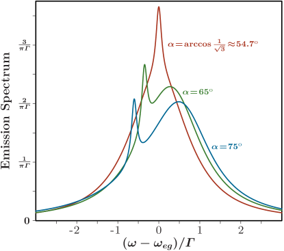
Figure 6: Emission spectra of a two-atom system in a strong magnetic field H at different values of the angle $\alpha$ at $k_{0}r=1$. All other preconditions are the same as in Fig. 2.

For the completeness, below we consider also the spectrum of the delayed fluorescence, measured at times much longer than the decay time $1/\Gamma_{s}$ through the symmetric channel.

IV.2.4 Spectrum of the delayed decay of the doubly excited system

Actually the delayed decay of the doubly excited two-atom system is a decay of a singly excited metastable state where the doubly excited system falls to (with a small probability [50)] after emission of a antisymmetric photon at an instant $t_{\textrm{in}}$ within a short time interval $~{}1/\Gamma_{s}$. This antisymmetric state is a superposition containing all possible polarizations and wave vectors of the emitted photon:

$$|\varPsi(t_{\textrm{in}})\rangle=\sideset{}{{}^{\prime}}{\sum}_{{\bf{k}},\lambda,j}B^{(a)}_{{\bf{k}}\lambda j}|\psi^{a}_{j}\rangle\otimes b^{{\dagger}}_{\lambda a}({\bf{k}})|{\textsl{vac}}\rangle\,,$$ (56)

where the amplitudes $B^{(a)}_{{\bf{k}}\lambda j}$ are given by Eq. (49). The state (56) may be considered as an “initial state” ($t_{\textrm{in}}\approx 0$) of further time evolution. This evolution may, in principle, be described by the wave function (44) with only antisymmetric components and with $A(t>t_{\textrm{in}})=0$. However, such a representation is not convenient for calculation of the delayed spectrum, because the state (56) keeps information about the primary photon emitted at the time $t_{\textrm{in}}$, while the delayed spectrum is measured at a considerably later time, when the primary photon is already far from the registration region. It is difficult to distinguish between the the primary and secondary photons in the framework of Schrödinger state evolution. To overcome this problem we develop the density matrix approach which eliminates excessive information about the primary photon.

The initial density matrix operator $\hat{\rho}_{\textrm{in}}$ of the atomic subsystem is determined by the state (56):

$$\hat{\rho}_{\textrm{in}}={\mathrm{Tr}}_{\textrm{ph}}\left\{|\varPsi(t_{\textrm{in}})\rangle\langle\varPsi(t_{\textrm{in}})|\right\}\\ =\sideset{}{{}^{\prime}}{\sum}_{{\bf{k}},\lambda,j,j^{\prime}}B^{(a)}_{{\bf{k}}\lambda j}B^{(a)}_{{\bf{k}}\lambda j^{\prime}}|\psi^{a}_{j}\rangle\langle\psi^{a}_{j^{\prime}}|\;,$$ (57)

where the trace is taken over the photon degrees of freedom. This operation allows one to forget about a primary photon emitted at the early time $t_{\textrm{in}}$, but the price paid is that the matrix $\hat{\rho}_{\textrm{in}}$ corresponds not to a pure but to a mixed state. The initial density matrix $\widehat{R}_{\textrm{in}}$ of the whole atomic-photon system is constructed as a direct product of the atomic density matrix $\hat{\rho}_{\textrm{in}}$ and the density matrix $|{\textsl{vac}}\rangle\langle{\textsl{vac}}|$ of photon vacuum:

$$\widehat{R}_{\textrm{in}}=\hat{\rho}_{\textrm{in}}\otimes|{\textsl{vac}}\rangle\langle{\textsl{vac}}|\;.$$ (58)

The further temporal dynamics of the system is governed by the Liouville equation:

$$i\frac{d}{dt}\widehat{R}(t)=[\widehat{\mathcal{H}}_{a},\widehat{R}]\,.$$ (59)

for the system density matrix $\widehat{R}(t)$ with the initial condition $\widehat{R}(t=0)=\widehat{R}_{\textrm{in}}$. The Hamiltonian $\widehat{\mathcal{H}}_{a}$ in (59) is the sum of the atom Hamiltonian $\widehat{H}^{(1)}_{a}$ (7), the $a$-part of the photon Hamiltonian (34), and the $a$-part of the interaction Hamiltonian (35):

$$\widehat{\mathcal{H}}_{a}=\sideset{}{{}^{\prime}}{\sum}_{{\bf{k}},\lambda}\hbar\omega(k)b_{\lambda a}^{{\dagger}}({\bf{k}})b_{\lambda a}({\bf{k}})+\sum_{j}E_{j}|\psi_{j}^{a}\rangle\langle\psi_{j}^{a}|\\ +\sideset{}{{}^{\prime}}{\sum}_{{\bf{k}},\lambda,j}[F_{{\bf{k}}\lambda}^{j}|\psi_{j}^{a}\rangle\langle g,g|b_{\lambda a}({\bf{k}})+\mathrm{H.c.}]\;,$$ (60)

where

$$F_{{\bf{k}}\lambda}^{j}=2i\sum_{m}g_{{\bf{k}}\lambda}^{m}\sin\left({\frac{{\bf{kr}}}{2}}\right)C_{mj}^{a}\,.$$ (61)

It should be noted that the developed formalism describes a “conditional” evolution of the system—under the condition that the decay goes through the antisymmetric channel. This is why the traces of the initial density matrices $\hat{\rho}_{\textrm{in}}$ and $\widehat{R}_{\textrm{in}}$ equal not to unity but to the probability (50) of falling to the antisymmetric channel.

In terms of the density matrix ${\widehat{R}}(t)$, the spectrum of the delayed fluorescence in the direction $\widehat{{\bf{k}}}$ is given by

$$S(\omega,\widehat{{\bf{k}}})\simeq\sum_{\lambda}\mathrm{Tr}\left\{b_{\lambda a}^{{\dagger}}({\bf{k}})b_{\lambda a}({\bf{k}})\widehat{R}(t)\right\}_{t\rightarrow\infty;\,k=\omega/c}\,,$$ (62)

where it is assumed that the measurement is performed during the time interval $(t_{1},t_{2})$ with $1/\Gamma_{s}\ll t_{1}\ll 1/\Gamma_{a}\ll t_{2}$.

The matrix $\widehat{R}$ can be represented in the form

$$\widehat{R}(t)=\sum_{j,j^{\prime}}\mathcal{A}_{jj^{\prime}}(t)|\psi_{j}^{a}\rangle\langle\psi_{j^{\prime}}^{a}|\otimes|{\textsl{vac}}\rangle\langle{\textsl{vac}}|\\ +\sideset{}{{}^{\prime}}{\sum}_{{\bf{k}},\lambda,j}[\mathcal{B}^{j}_{{\bf{k}}\lambda}(t)|g,g\rangle\langle\psi_{j}^{a}|\otimes|{\bf{k}}\lambda\rangle\langle{\textsl{vac}}|+\mathrm{H.c.}]\\ +\sideset{}{{}^{\prime}}{\sum}_{{\bf{k}},\lambda,{\bf{k}}^{\prime},\lambda^{\prime}}\mathcal{D}_{{\bf{k}}\lambda;{\bf{k}}^{\prime}\!\lambda^{\prime}}(t)|g,g\rangle\langle g,g|\otimes|{\bf{k}}\lambda\rangle\langle{\bf{k}}^{\prime}\!\lambda^{\prime}|\;,$$ (63)

where $|{\bf{k}}\lambda\rangle=b_{\lambda a}({\bf{k}})|{\textsl{vac}}\rangle$. The initial condition $\widehat{R}(t=0)=\widehat{R}_{\textrm{in}}$ takes the form: $\mathcal{A}_{jj^{\prime}}(0)=(\hat{\rho}_{\textrm{in}})_{jj^{\prime}}$, $\mathcal{B}^{j}_{{\bf{k}}\lambda}(0)=0$, $\mathcal{D}_{{\bf{k}}\lambda;{\bf{k}}^{\prime}\!\lambda^{\prime}}(0)=0$. In this representation, the spectrum has the form:

$$S(\omega,\widehat{\bf{k}})=\sum_{\lambda}\mathcal{D}_{{\bf{k}}\lambda;{\bf{k}}\lambda}(t\rightarrow\infty)|_{k=\omega/c}\,.$$ (64)

The Liouville equation (59) leads to a system of linear differential equations for the amplitudes entering the representation (63). These equations can be solved by the Laplace transform, a bit boring but straightforward calculations. In principle, this allows one to find arbitrary correlation functions of the emitted light including the spectrum (64).

However, the main features of the delayed spectrum can be understood based on the presented here scenario of the decay. Namely, the spectrum consists of three very narrow peaks of widths $\sim\Gamma_{aj}$ (41); the peaks’ centers correspond to energies of three antisymmetric singly-excited states ($j=-1,0,1$) of the atomic subsystem in the magnetic field. The peak weight $I_{j}$ (i.e., the emission power collected from all the angles and integrated over frequencies within the peak widths) is proportional to the initial population $P_{j}$ of the state $j$: $I_{j}\propto P_{j}\equiv(\hat{\rho}_{\textrm{in}})_{jj}$. The latter quantity is calculated with the use of Eqs. (49) (57) (see Eq. (A26) in Appendix A). In the case of our major interest, when the angle $\alpha$ between the vector connecting the two atoms and the magnetic field is a magic one, Eq. (A26) takes a simple form:

$$P_{j}={\frac{1}{12}}|k_{0}r|^{2}|C^{a}_{mj}|^{2}\,,$$ (65)

where the index $m$ characterizes the original doubly excited state $|m,m\rangle$, and the matrix $\widehat{C}^{a}$ is determined by Eqs. (17), (21), and (22). Here we give ratios of the peak weights for the considered decay of the doubly excited state $|0,0\rangle$ prepared by a linearly polarized $\pi$-pulse:

$$I_{-1}:I_{0}:I_{1}\\ =\left[\frac{q_{-1}(E^{a}_{-1}+U_{r})}{\varOmega_{H}+E^{a}_{-1}+U_{r}}\right]^{2}:q^{2}_{0}:\left[\frac{q_{+1}(E^{a}_{1}+U_{r})}{\varOmega_{H}-E^{a}_{1}-U_{r}}\right]^{2}\;,$$ (66)

where $E^{a}_{j}$ and $q_{j}$ are determined by Eqs. (11) and (22), respectively. An example of the dependence of peak weights on the magnitude of the magnetic field is shown in Fig. 7.

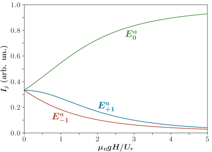
Figure 7: Magnetic field dependence of the intensities $I_{j}$ of peaks of the delayed fluorescence (see the text) at the frequencies $E_{j}^{a}/\hbar$. Their ratios are defined by Eq. (66), and they are normalized so that $\sum_{j}I_{j}=1$. The field ${\bf{H}}$ is directed at the angle $\alpha=\alpha_{\textrm{mag}}$ relative to the vector separation ${\bf{r}}$ between the atoms. Initially excited state is $|m=0,m=0\rangle$.

Using the developed formalism one can also calculate the integral intensities $I_{j}({\widehat{{\bf{k}}}})$ of the lines at the frequencies $E_{j}^{a}/\hbar$ for an arbitrary direction ${\widehat{{\bf{k}}}}$ of observation. These quantities and the relation between them turn out to depend on ${\widehat{{\bf{k}}}}$.

V Determination of the mutual orientation of the two atoms

Sensitivity of the fluorescence spectrum of the doubly excited system to the angle $\alpha$ between the vector separation ${\bf{r}}$ and the magnetic field ${\bf{H}}$ (see Sec. IV.2.3 and Fig 2) allows one to find the direction of ${\bf{r}}$ from an experiment. As follows from Eq. (55) the positions of the broad and narrow central peaks almost coincide when $\alpha\approx\alpha_{mag}$. Thus, rotating the direction of the magnetic field (while keeping the propagation direction and polarization of the pumping light orthogonal and parallel to the magnetic field, respectively) and measuring the emission spectrum, one can find the configuration where the positions of two peaks in Fig. 2 (or in Fig. 6) coincide. This means that the angle between the found direction ${\mathbf{\widehat{h}}}_{1}$ of the magnetic field ${\bf{H}}$ and the separation vector ${\bf{r}}$ equals to the magic angle $\alpha_{\textrm{mag}}$. However, this condition determines not the direction $\widehat{\mathbf{r}}$ of $\bf{r}$ but the whole cone of possible directions (see Fig. 8a). To find $\widehat{\mathbf{r}}$ one should repeat the routine searching for some other suitable direction $\widehat{\mathbf{h}}_{2}$ of the magnetic field such that the two spectral peaks coincide, so that ${\widehat{\mathbf{r}}}{\widehat{\mathbf{h}}}_{2}=\cos\alpha_{\textrm{mag}}$. From these measurements and the elementary geometrical analysis presented in Appendix C, one finds the desired vector $\widehat{\mathbf{r}}$ between the atoms in the form:

$$\widehat{\mathbf{r}}=\frac{\cos{(\alpha_{\textrm{mag}})}}{1+\cos{\vartheta_{12}}}[\widehat{\mathbf{h}}_{1}+\widehat{\mathbf{h}}_{2}]\\ \pm\frac{1}{\sin{\vartheta_{12}}}\sqrt{1-\frac{2\cos^{2}{(\alpha_{\textrm{mag}})}}{1+\cos{\vartheta_{12}}}}[\widehat{\mathbf{h}}_{1}\times\widehat{\mathbf{h}}_{2}]\,,$$ (67)

where $\vartheta_{12}$ is the angle between $\widehat{\mathbf{h}}_{1}$ and $\widehat{\mathbf{h}}_{2}$. The remaining uncertainty [due to the $\pm$ sign in Eq. (67)] can be eliminated by repeating the routine and finding the third suitable direction $\widehat{\mathbf{h}}_{3}$ of the magnetic field.

The described procedure presents an example of determining the direction of the vector separation. Another possibility is shown in Fig. 8.

As described in Sec. IV.2.2, the information about the length of $\bf{r}$ can be extracted by measuring the ratio of the quantum yields of the fast and the delayed fluorescence and using Eq. (50). Together with the information about the direction of $\bf{r}$ [Eq. (67)] this provides full knowledge about the relative arrangement of two atoms.

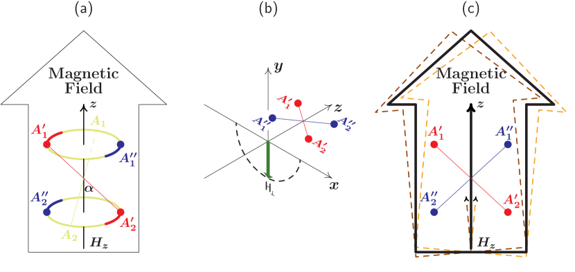
Figure 8: Determination of the direction of the vector separation ${\bf{r}}$ using subsequently three configurations of the magnetic fields. (a) Superimposition of the narrow and broad peaks of the spectrum in Fig. 2 by varying of the H direction leads to determination of the cone of possible directions of ${\bf{r}}$ and fixes the axis $z$. (b) The rotation of ${\bf{H}}_{\perp}$ in the plane perpendicular to $z$ allows one to fix the axises $x$ and $y$ when the separation of the two peaks is maximal, i.e., the angle between ${\bf{H}}_{\perp}$ and ${\bf{r}}$ equals to $\pi/2$. (c) The choice between the two remaining possible directions can be made by slight deflection of the ${\bf{H}}$ direction from $z$—as seen from Fig. 2 the counter clockwise deflection leads to the red shift of the narrow peak, and vice versa.

VI Conclusion

We have described fluorescence of an excited system of two closely located identical atoms, each atom having a non-degenerate ground state $|g\rangle$ of the angular momentum $J=0$ and a triply degenerate excited state $|J=1,m=0,\pm 1\rangle$. We accounted for the resonant dipole-dipole interaction between close atoms and its competition with the Zeeman splitting of the levels in an external magnetic field. The fluorescence spectrum and its time behavior depend on the strength and direction of the magnetic field. The emission of a doubly excited system possesses two very different time regimes: for the ensemble, fast strong emission pulse (of the duration $\sim 1/\varGamma_{s}$) is followed by a weak but long (of the duration $\sim 1/\varGamma_{a}$) fluorescence from metastable states where the system can fall with a small but finite probability after the excitation. A very sensitive dependence of the fluorescence spectrum on the direction of the magnetic field allows one to determine the direction of the vector connecting the two atoms. On the other hand, measuring the ratio of the fast and the delayed emission powers one can extract the information about the distance between the two atoms. Thus, one can get a complete information about the relative position of two atoms at nanoscale by entirely optical means.

We have studied the simplest realistic two-particle model. A similar analysis may be applied to other systems: quantum dots, color centers, molecules in matrices, etc.

Appendix A: Details on interaction with the electromagnetic field

We use the standard representation of the electric field operator in terms of the photon creation and annihilation operators $a^{{\dagger}}_{{\bf k},\lambda}$ and $a_{{\bf k},\lambda}$:

$${\widehat{{\bf{E}}}}({\bf{r}})=\sum_{{\bf{k}},\lambda}\sqrt{\frac{2\pi\hbar\omega_{k}}{V}}\left[e^{i{\bf{kr}}}{\bf{e}}_{{\bf{k}}\lambda}a_{{\bf{k}}\lambda}+\mathrm{H.c.}\right]\;,$$ (A1)

where $V$ is the quantization volume, ${\bf{e}}_{{\bf{k}}\lambda}$ is the polarization vector ($\lambda=1,\,2$) of the photon of a wave vector ${\bf{k}}$ and frequency $\omega_{k}$. In the dipole approximation, the atom-field interaction operator is $-{\widehat{{\bf{d}}}}\!\!\cdot\!\!{\widehat{{\bf{E}}}}$. Its matrix element corresponding in RWA to the atom transition $|g\rangle\leftrightarrow|m\rangle$ ($g$ is the ground state, and $|m\rangle$ is one of the excited states $|e^{(m)}\rangle$ with $m=0,\pm 1$) is given by

$$g_{{\bf{k}}\lambda}^{m,g}=\sqrt{\frac{2\pi\hbar\omega_{k}}{V}}\langle m|{\widehat{{\bf{d}}}}|g\rangle{\bf{e}}_{{\bf{k}}\lambda}\;.$$ (A2)

Using RWA, we can replace the photon frequency $\omega_{k}$ in Eq. (A2) by the resonance transition frequency $\omega_{eg}$. In the considered model of atom levels (of the angular momentum $J=0$ in the ground state, and $J=1$ in the excited ones), the corresponding wave functions have a structure typical for a particle in a centrosymmetric field: $\Phi_{J=0}({\bf{r}})=R_{0}(r)$, $\Phi_{J=1,m=\pm 1}({\bf{r}})=R_{1}(r)\sin{\theta_{{\bf{r}}}}e^{\pm i\varphi_{{\bf{r}}}}$, $\Phi_{J=1,m=0}({\bf{r}})=\sqrt{2}R_{1}(r)\cos{\theta_{{\bf{r}}}}$, where $\theta_{{\bf{r}}}$ and $\varphi_{{\bf{r}}}$ are the polar and the azimuthal angles of the radius-vector ${\bf{r}}$, $R_{0}(r)$ and $R_{1}(r)$ are the radial functions in the ground and excited states, respectively. Non-zero matrix elements $\langle m|{\widehat{\bf{d}}}|g\rangle$ can be expressed in terms of a single quantity $d_{0}\equiv\langle 0|\hat{d}_{z}|g\rangle$, namely: $\langle\pm 1|\hat{d}_{\pm}|g\rangle=\sqrt{2}d_{0}$, where $\hat{d}_{\pm}\equiv\hat{d}_{x}\pm i\hat{d}_{y}$.

For calculations one should specify the choice of the polarization vectors. Representing Cartesian coordinates of a wave vector ${\bf{k}}$ in the form

$${\bf{k}}=|{\bf{k}}|(\sin{\theta}\cos{\varphi},\sin{\theta}\sin{\varphi},\cos{\theta})\;,$$ (A3)

where $\theta$ and $\varphi$ are the polar and the azimuthal angles in the momentum space, we choose two vectors of the linear polarization in the following form:

$${\bf{e}}_{{\bf k}1}=(-\sin{\varphi},\,\cos{\varphi},\,0)\;,\\$$ (A4)

$${\bf{e}}_{{\bf{k}}2}=\frac{[{\bf{k}}\times{\bf{e}}_{{\bf{k}}1}]}{\Big{|}[{\bf{k}}\times{\bf{e}}_{{\bf{k}}2}]\Big{|}}=(\cos{\varphi}\cos{\theta},\,\sin{\varphi}\cos{\theta},\,-\sin{\theta})\,.$$ (A5)

It is easy to check that these vectors are perpendicular to each other and to k. Then the matrix elements (A2) take the form:

$$\left\{\begin{array}[]{c}g_{{\bf{k}}1}^{\pm 1,g}\\ g_{{\bf{k}}2}^{\pm 1,g}\end{array}\right\}={\sqrt{{\frac{\pi\hbar\omega_{eg}}{V}}}}d_{0}e^{\mp i\varphi}\left\{\begin{array}[]{c}\mp i\\ \cos\theta\end{array}\right\}\;,$$ (A6)

$$g_{{\bf{k}}1}^{0,g}=0\;,\;\;\;\;g_{{\bf{k}}2}^{0,g}=-{\sqrt{{\frac{2\pi\hbar\omega_{eg}}{V}}}}d_{0}\sin{\theta}\;.$$ (A7)

Replacing the original set of photon operators $a_{{\bf{k}}\lambda}$ used in the Hamiltonians (III) and (III) by the properly symmetrized operators (28)–(31), one should restrict the space of photon wave vectors by the upper hemisphere ($k_{z}\geqslant 0$) to avoid double counting and to provide the correct hold true the commutation relations (32). Correspondingly, in the transformation of Hamiltonians from (III) and (III) to (35) and (36) we used the symmetry properties of the polarization vectors (A4) and (A5): ${\bf{e}}_{-{\bf{k}},1}=-{\bf{e}}_{{\bf{k}},1}$ and ${\bf{e}}_{-{\bf{k}},2}={\bf{e}}_{{\bf{k}},2}$.

For further references we write down a useful relation:

$$\sum_{\lambda}g_{{\bf{k}}\lambda}^{m,g}(g_{{\bf{k}}\lambda}^{m^{\prime},g})^{*}=\frac{\pi\hbar\omega_{eg}d^{2}_{0}}{V}G_{mm^{\prime}}\;,\;\;\;\;\;\;G_{mm^{\prime}}=\begin{pmatrix}1+\cos^{2}\theta&-\sqrt{2}\sin{\theta}\cos{\theta}e^{i\varphi}&-\sin^{2}{\theta}e^{2i\varphi}\\ -\sqrt{2}\sin{\theta}\cos{\theta}e^{-i\varphi}&2\sin^{2}{\theta}&-\sqrt{2}\sin{\theta}\cos{\theta}e^{i\varphi}\\ -\sin^{2}{\theta}e^{-2i\varphi}&-\sqrt{2}\sin{\theta}\cos{\theta}e^{-i\varphi}&1+\cos^{2}\theta\end{pmatrix}$$ (A8)

that directly follows from equations (A4)–(A7).

1. Decay of a singly excited state of the two-atom system

Consider the two-atom system prepared at the time $t=0$ in one of the eigenstates $\psi^{\nu}_{j}$ of a definite symmetry $\nu=s,a$. The time evolution of the atom-photon system is described by the wave function (37), that obeys the Schrödinger equation with the Hamiltonian (III). It is convenient to represent $|\varPsi(t)\rangle$ in the form $\exp(-iE^{\nu}_{j}t)|\widetilde{\varPsi}(t)\rangle$ with slowly varying amplitudes. After the Laplace transformation

$$|\varPsi(t)\rangle\rightarrow|\varPsi[z]\rangle=\int_{0}^{\infty}\,dt\,e^{-zt}|\varPsi(t)\rangle\;,$$ (A9)

the Schrödinger equation for (37) can be written as the system of equations for the Laplace transforms of the slowly varying amplitudes their symbol tilde is omitted for brevity):

$$\begin{split}&[z+i(\omega_{k}-E^{\nu}_{j})]B^{\nu}_{{\bf{k}}\lambda}[z]=2iA^{\nu}_{j}[z]f^{*}_{\nu}({\bf{kr}})\sum_{m}(g^{m,g}_{{\bf{k}}\lambda}C^{\nu}_{mj})^{*}\;,\\ &zA_{j}^{\nu}[z]=1+2i\sideset{}{{}^{\prime}}{\sum}_{{\bf{k}},\lambda,m}g^{m,g}_{{\bf{k}}\lambda}C^{\nu}_{mj}f_{\nu}({\bf{kr}})B^{\nu}_{{\bf{k}}\lambda}[z]\;,\end{split}$$ (A10)

where $f_{\nu}(\xi)=\cos{\xi/2}$ for $\nu=s$ and $f_{\nu}(\xi)=i\sin{\xi/2}$ for $\nu=a$. It is assumed that the energy differences between the levels $E^{\nu}_{j}$ of the atomic system are large as compared with the radiative widths of these levels. This is why the system (A10) ignores mixing of states with different $j$. Representing $B^{\nu}_{\vec{k}\lambda}[z]$ in terms of $A^{\nu}_{j}[z]$ we obtain the following equation for $A^{\nu}_{j}[z]$:

$$\left[z\!+\!\!\sum_{m,m^{\prime}}\sideset{}{{}^{\prime}}{\sum}_{{\bf{k}},\lambda}\frac{4g^{m,g}_{{\bf{k}}\lambda}C^{\nu}_{mj}|f_{\nu}({\bf{kr}})|^{2}(g^{m^{\prime},g}_{{\bf{k}}\lambda}C^{\nu}_{m^{\prime}j})^{*}}{z+i(\omega_{{\bf{k}}}-E^{\nu}_{j})}\right]\!A^{\nu}_{j}[z]\!\!=\!\!1\;.$$ (A11)

The second term in the square brackets describes both the radiative width and the energy shift. Neglecting the latter we represent (A11) as $[z+\varGamma_{\nu j}/2]A^{\nu}_{j}[z]=1$, where the term $\varGamma_{\nu j}/2$ results from the pole integration over $\omega_{k}$ near the resonance $\omega_{k}\approx E^{\nu}_{j}$:

$$\varGamma^{\nu}_{j}=4\omega^{3}_{0}d^{2}_{0}\int^{\prime}\frac{d\hat{o}}{4\pi}|f_{\nu}({\bf{kr}})|^{2}\sum_{m,m^{\prime}}G_{mm^{\prime}}C^{\nu}_{mj}C^{{\nu}*}_{m^{\prime}j}\;.$$ (A12)

Here Eq. (A8) is used, and the integration is performed over the hemisphere in the polar angles $\theta$ ($0\leqslant\theta\leqslant\pi/2$) and $\varphi$ $0\leqslant\varphi\leqslant 2\pi$) that describe directions of the photon wave-vector ${\bf{k}}$ while its length is kept constant ($|{\bf{k}}|=k_{0}=\omega_{eg}/c$), and $d{\hat{o}}=\sin\theta\,d\theta\,d\varphi$.

Let us consider first the decay of a symmetric state ($\nu=s$). For closely located atoms one has $f_{s}({\bf{kr}})=\cos({\bf{kr}}/2)\approx 1$. The angular integration in (A12) results in $\int^{\prime}G_{mm^{\prime}}d\hat{o}/(4\pi)=(2/3)\delta_{mm^{\prime}}$, so the remaining summation of $C^{s}_{mj}C^{s*}_{mj}$ over $m$ gives unity due to that the matrix $\widehat{C}$ is unitary. So, we arrive at the expression $\varGamma^{s}_{j}=8\omega^{3}_{0}d^{2}_{0}/3\hbar c^{3}=2\varGamma$, presented by Eqs. (38) and (39) in the main text. Thus, the decay rate of the symmetric states is a robust quantity insensitive to the magnetic field.

For antisymmetric states ($\nu=a$) the situation is more complicated. Using the definition of ${\bf{r}}$ in the beginning of the Sec. II and also Eq. (A3), the function $f_{a}({\bf{kr}}/2)$ entering Eq. (A12) is approximated as $ik_{0}r[\sin{\alpha}\sin{\theta}\cos{\varphi}+\cos{\alpha}\cos{\theta}]/2$. Then the expression (A12) for $\varGamma^{a}_{j}$ takes the form

$$\varGamma^{a}_{j}=\frac{3}{4}\varGamma k^{2}_{0}r^{2}\sum_{m,m^{\prime}}\mathcal{G}_{mm^{\prime}}C^{a}_{mj}(C^{{a}}_{m^{\prime}j})^{*}\;,$$ (A13)

where

$$\mathcal{G}_{mm^{\prime}}=\frac{1}{4\pi}\int\limits^{{\frac{\pi}{2}}}_{0}\sin{\theta}\int\limits^{2\pi}_{0}\frac{({\bf{kr}})^{2}}{k^{2}r^{2}}G_{mm^{\prime}}\,d\varphi\,d\theta\;.$$ (A14)

Direct calculation gives for (A14)

$$\mathcal{G}_{mm^{\prime}}\!\!=\!\!\begin{pmatrix}{\frac{1}{30}}(7+\cos 2\alpha)&-\frac{\sqrt{2}}{30}\sin 2\alpha&-\frac{1}{15}\sin^{2}{\alpha}\\ -\frac{\sqrt{2}}{30}\sin 2\alpha&{\frac{1}{15}}(3-\cos 2\alpha)&-\frac{\sqrt{2}}{30}\sin 2\alpha\\ -\frac{1}{15}\sin^{2}\alpha&-\frac{\sqrt{2}}{30}\sin 2\alpha&{\frac{1}{30}}(7+\cos 2\alpha)\end{pmatrix}\;.$$ (A15)

This expression simplifies for the magic angle $\alpha_{\mathrm{mag}}=\arccos{(1/\sqrt{3})}$:

$$\mathcal{G}_{mm^{\prime}}=\frac{2}{9}\left[{\widehat{\mathbb{I}}}-\frac{1}{5}\left(\begin{array}[]{ccc}0&1&1\\ 1&0&1\\ 1&1&0\\ \end{array}\right)\right]\,,$$ (A19)

where ${\widehat{\mathbb{I}}}$ is the unit matrix. Eqs. (A13) and (A19) lead to the above announced expressions (41) and (42).

2. Decay of a doubly excited state of the two-atom system

Here we give more detail on the derivation of the results presented in section IV.2.1. The decay of a doubly excited state, e.g., the state $|0,0\rangle$ (i.e., $m_{1}=m_{2}=0$) of the two-atom system is described by a quite complicated system of Schrödinger equations for the probability amplitudes entering Eq. (44). However, the analysis of the system evolution can be simplified due to the great difference $\varGamma_{s}\gg\varGamma_{a}$ between the decay rates in the symmetric and antisymmetric channels, see Fig. 4. This allows one to describe the time evolution in the following succession of steps. At the first step, neglecting the existence of the slow antisymmetric channel we find the time evolution of the amplitude $A(t)$ in Eq. (44). At the second step, using this fast decaying function $A(t)$ we calculate a small probability of emission of a single antisymmetric photon. Once occurred, this event determines further evolution of the system via the antisymmetric channel.

Step 1. Decay rate via the symmetric channel. The time dependence of $A(t)$ is mainly determined by the first transition of the decay, see Fig. 4. Using the Hamiltonian (36), we obtain equations for the Laplace transforms of the slow amplitudes ${\bar{A}}(t)=A(t)e^{2i\omega_{eg}t}$ and $\bar{B}^{s}_{{\bf{k}}\lambda j}=B^{s}_{{\bf{k}}\lambda j}e^{2i\omega_{eg}t}$ as

$$[z+i(\omega_{{\bf{k}}}+E^{s}_{j}-2\omega_{eg})]\bar{B}^{s}_{{\bf{k}}\lambda j}[z]\\ =2i(g^{m=0,g}_{{\bf{k}}\lambda}C^{s}_{m=0,j})^{*}\bar{A}[z]+...\;,\\ z\bar{A}[z]=1+2i\sideset{}{{}^{\prime}}{\sum}_{{\bf{k}},\lambda,j}g^{m=0,g}_{{\bf{k}}\lambda}C^{s}_{m=0,j}\bar{B}^{s}_{{\bf{k}},\lambda,j}[z]\;,$$ (A20)

where we put $\cos({\bf{kr}}/2)\approx 1$. The omitted terms in the first equation correspond to transitions from the singly excited symmetric states (of energies $E^{s}_{j}$) to the ground state, they give only negligible corrections to the studied decay rate of the doubly excited state. From the above system we express $\bar{B}^{s}_{{\bf{k}}\lambda j}$ in terms of $\bar{A}[z]$, put it into the last equation and perform a pole integration over $\omega_{{\bf{k}}}$. In this way we arrive at the reduced equation for $\bar{A}[z]$:

$$[z+\varGamma_{2s}/2]\tilde{A}[z]=1\;,$$ (A21)

where

$$\varGamma_{2s}=4\omega^{3}_{0}d^{2}_{0}\sum_{j}C^{s}_{m=0,j}\!\left(C^{{s}}_{m^{\prime}=0,j}\right)^{*}\int^{\prime}\frac{d\hat{o}}{4\pi}G_{0,0}(\theta,\varphi)\;,$$ (A22)

and the summation rule (A8) is used. The summation in $j$ gives unity due to the unitarity of the matrix $\widehat{C}^{s}$. Performing the angle integration over the upper hemisphere we find the expected relation [see Eq. (47)]: $\varGamma_{2s}=\varGamma_{s}=2\varGamma$.

Step 2. Leakage to the antisymmetric channel [derivation of Eqs. (48)–(50)]. Now our aim is to find the probability amplitudes $B^{a}_{{\bf{k}}\lambda j}$ [see Eq. (44)] of the antisymmetric states where the doubly excited system may fall after the emission of an antisymmetric photon. The short-time evolution of these amplitudes is mainly governed by the antisymmetric part of the Hamiltonian (36) that connect these antisymmetric states with the doubly excited one (see Fig. 4):

$$\left[i{\frac{\partial}{\partial t}}-(E^{a}_{j}+\omega_{k})\right]B^{a}_{{\bf{k}}\lambda j}(t)\\ =2i\left(g^{m=0,g}_{{\bf{k}}\lambda}C^{a}_{m=0,j}\right)^{*}\sin{\left(\frac{{\bf{kr}}}{2}\right)}A(t)\;,$$ (A23)

where the amplitude $A(t)$ is determined by the symmetric decay channel as in Eq. (47). The solution of Eq. (A23) with the initial condition $B^{a}_{{\bf{k}}\lambda j}(t=0)=0$ is given by

$$B^{a}_{{\bf{k}}\lambda j}(t)=-{\frac{2i\left(g^{m=0,g}_{{\bf{k}}\lambda}C^{a}_{m=0,j}\right)^{*}\sin\left({\frac{{\bf{kr}}}{2}}\right)}{E^{a}_{j}+\omega_{{\bf{k}}}-2\omega_{eg}+i\varGamma}}\\ \times\left[e^{-(2i\omega_{eg}+\varGamma)t}-e^{-i(E^{a}_{j}+\omega_{{\bf{k}}})t}\right]\;.$$ (A24)

When time $t$ is much greater than $1/\varGamma$ (but is still much shorter than the antisymmetric decay time $~{}1/\varGamma^{a}$), this expression reduces to Eq. (49).

Now we derive the diagonal elements of the initial density matrix (57) of the atomic subsystem (after the emission of a single antisymmetric photon):

$$P_{j}=\langle\psi^{a}_{j}|\hat{\rho}_{\textrm{in}}|\psi^{a}_{j}\rangle=\sideset{}{{}^{\prime}}{\sum}_{{\bf{k}},\lambda}\left|B^{a}_{{\bf{k}}\lambda j}\left(\frac{1}{\varGamma}\ll t\lesssim\frac{1}{\varGamma^{a}}\right)\right|^{2}\\ =\sideset{}{{}^{\prime}}{\sum}_{{\bf{k}},\lambda}\frac{4|g^{m=0,g}_{{\bf{k}}\lambda}C^{a}_{m=0,j}|^{2}}{(\omega_{{\bf{k}}}+E^{a}_{j}-2\omega_{eg})^{2}+\varGamma^{2}}\sin^{2}{\left(\frac{\bf{kr}}{2}\right)}\,.$$ (A25)

Performing here the pole integration in $\omega_{k}$ and using the summation rule (A8), we obtain

$$P_{j}=\frac{3}{8}k^{2}_{0}r^{2}|C^{a}_{m=0,j}|^{2}\mathcal{G}_{0,0}(\alpha)\;,$$ (A26)

where the approximation $\sin{x}\approx x$ is used, the matrix $\mathcal{G}_{m,m^{\prime}}(\alpha)$ is given by Eq. (A15) for an arbitrary angle $\alpha$ and by Eq. (A19) for the magic angle. Using Eq. (A19), we arrive at the result for $P_{j}$, Eq. (65). Finally, the total probability for the doubly excited system to follow the antisymmetric decay channel is given by the summation of (A26) in $j$. Due to the unitarity of the matrix $\widehat{C}^{a}$ we arrive at

$$P=\sum_{j}P_{j}=\frac{3}{8}k^{2}_{0}r^{2}\mathcal{G}_{0,0}(\alpha)\,.$$ (A27)

In general, this probability depends on the angle $\alpha$ as $P\propto(3-\cos 2\alpha)$. For the magic angle $\alpha_{mag}$ we arrive at the expression (50).

Appendix B: Derivation of Eq. (54) for the spectrum of spontaneous emission in a strong magnetic field

For the spontaneous decay in a strong magnetic field of a doubly excited state $|m_{1}=0,m_{2}=0\rangle$, the wave function (44) can be reduced to

$${}\varPsi(t)=A(t)|0,0\rangle\otimes|{\textsl{vac}}\rangle+\int{\widetilde{B}}_{{s}}(\omega_{1s},t)|s_{0}\rangle\otimes|{\textsl{1}}_{\omega_{1s}}\rangle\,d\omega_{1s}+\int{\widetilde{B}}_{{a}}(\omega_{1a},t)|a_{0}\rangle\otimes|{\textsl{1}}_{\omega_{1a}}\rangle\,d\omega_{1a}\\ +\int\!\!\!\int_{\omega_{1s}\leqslant\omega_{2s}}{\widetilde{C}}_{s}(\omega_{1s},\omega_{2s},t)|g,g\rangle\otimes|{\textsl{1}}_{\omega_{1s}}{\textsl{1}}_{\omega_{2s)}}\rangle\;d\omega_{1s}d\omega_{2s}+\int\!\!\!\int_{\omega_{1a}\leqslant\omega_{2a}}{\widetilde{C}}_{a}(\omega_{1a},\omega_{2a},t)|g,g\rangle\otimes|{\textsl{1}}_{\omega_{1a}}{\textsl{1}}_{\omega_{2a}}\rangle\;d\omega_{1a}d\omega_{2a}\;.$$ (B1)

Here the following designations are used: (i) the one-photon wave packets $|{\textsl{1}}_{\omega s}\rangle$ and $|{\textsl{1}}_{\omega a}\rangle$ are introduced being the unique superpositions of the corresponding symmetric and antisymmetric one-photon states $b^{\dagger}({\bf{k}})|{\textsl{vac}}\rangle$ with different ${\bf{k}}$ (and the same $|{\bf{k}}|$), that alone interact with the state $m=0$ FANO_MAK ; (ii) $|{\textsl{1}}_{\omega_{1s}}{\textsl{1}}_{\omega_{2s}}\rangle$ and $|{\textsl{1}}_{\omega_{1a}}{\textsl{1}}_{\omega_{2a}}\rangle$ are two-photon states where $\omega_{1\nu}\leqslant\omega_{2\nu}$ is taken for definiteness; (iii) and indexes are simplified for the probability amplitudes ${\widetilde{B}}$ and ${\widetilde{C}}$ that replace $B$ and $C$; (iv) a shorter notation is used for the singly excited states, $|s_{0}=\left|\psi_{m=0}^{(\nu=s)}\right\rangle$ and $|a_{0}\rangle=\left|\psi_{m=0}^{(\nu=a)}\right\rangle$

The Shrödinger equation for the wave function (B1) is given by the following set of equations for the probability amplitudes (where $\varDelta$ is the splitting between the states $|s_{0}\rangle$ and $|a_{0}\rangle$):

$${}\begin{split}&{\frac{dA}{dt}}=-2i\omega_{eg}A-i\sqrt{{\frac{\varGamma_{{s}}}{2\pi}}}\int\limits_{-\infty}^{\infty}{\widetilde{B}}_{s}(\xi)\,d\xi-i\sqrt{{\frac{\varGamma_{{a}}}{2\pi}}}\int\limits_{-\infty}^{\infty}{\widetilde{B}}_{a}(\xi)\,d\xi\;,\\ &{\frac{d{\widetilde{B}}_{s}(\omega_{1s})}{dt}}=-i\left(\omega_{eg}+{\frac{1}{2}}\varDelta+\omega_{1s}\right){\widetilde{B}}_{s}-i\sqrt{{\frac{\varGamma_{{s}}}{2\pi}}}A-i\sqrt{{\frac{\varGamma_{{s}}}{2\pi}}}\left(\int\limits_{-\infty}^{\omega_{1s}}{\widetilde{C}}_{s}(\xi,\omega_{1s})\,d\xi+\int\limits_{\omega_{1s}}^{\infty}{\widetilde{C}}_{s}(\omega_{1s},\xi)\;d\xi\right)\;,\\ &{\frac{d{\widetilde{B}}_{a}(\omega_{1a})}{dt}}=-i\left(\omega_{eg}-{\frac{1}{2}}\varDelta+\omega_{1a}\right){\widetilde{B}}_{{a}}-i\sqrt{{\frac{\varGamma_{{a}}}{2\pi}}}A-i\sqrt{{\frac{\varGamma_{{a}}}{2\pi}}}\left(\int\limits_{-\infty}^{\omega_{1a}}{\widetilde{C}}_{a}(\xi,\omega_{1a})\,d\xi+\int\limits_{\omega_{1a}}^{\infty}{\widetilde{C}}_{a}(\omega_{1a},\xi)\;d\xi\right)\;,\\ &{\frac{d{\widetilde{C}}_{s}(\omega_{1s},\omega_{{2s}})}{dt}}=-i(\omega_{1s}+\omega_{2s}){\widetilde{C}}_{s}--i\sqrt{{\frac{\varGamma_{s}}{2\pi}}}\left[{\widetilde{B}}_{s}(\omega_{1s})+{\widetilde{B}}_{s}(\omega_{2s})\right]]\;,\\ &{\frac{d{\widetilde{C}}_{a}(\omega_{1a},\omega_{{2a}})}{dt}}=-i(\omega_{1a}+\omega_{2a}){\widetilde{C}}_{a}--i\sqrt{{\frac{\varGamma_{a}}{2\pi}}}\left[{\widetilde{B}}_{a}(\omega_{1a})+{\widetilde{B}}_{a}(\omega_{2a})\right]\;.\end{split}$$ (B2)

These equations incorporate the idealizations introduced by the Weisskopf–Wigner approximation WW : integrations in photon frequencies are performed from $-\infty$ to $+\infty$; non-diagonal matrix elements of the atom–field interaction do not depend on $\omega$, so, being expressed in terms of the spontaneous decay rates $\varGamma_{s}$ and $\varGamma_{a}$ [see Eqs. (38) and (40)], they are pulled out the corresponding integrals.

The initial condition of interest is

$${}\begin{split}A(t=0)=1\;,\;\;{\widetilde{B}}_{s}(t=0)={\widetilde{B}}_{a}(t=0)&=0\;,\\ {\widetilde{C}}_{s}(t=0)={\widetilde{C}}_{a}(t=0)&=0\;.\end{split}$$ (B3)

The solution of Eq. (B2) with the initial condition (B3) can be obtained by the method described in Ref. MAK_YUD . It is convenient to represent the solution in the following integral form that is easy to check:

$${}\begin{split}A=&{\frac{1}{2\pi i}}\int\limits_{-\infty}^{\infty}{\frac{e^{izt}\,dz}{z+2\omega_{eg}-{\frac{i}{2}}(\varGamma_{s}+\varGamma_{a})}}\;,\\ {\widetilde{B}}_{s}=&-{\frac{1}{2\pi i}}{\sqrt{{\frac{\varGamma_{s}}{2\pi}}}}\int\limits_{-\infty}^{\infty}{\frac{e^{izt}\,dz}{\left[z+2\omega_{eg}-{\frac{i}{2}}(\varGamma_{s}+\varGamma_{a})\right]\left(z+\omega_{eg}+{\frac{1}{2}}\varDelta-{\frac{i}{2}}\varGamma_{s}+\omega_{1s}\right)}}\;,\\ {\widetilde{B}}_{a}=&-{\frac{1}{2\pi i}}{\sqrt{{\frac{\varGamma_{a}}{2\pi}}}}\int\limits_{-\infty}^{\infty}{\frac{e^{izt}\,dz}{\left[z+2\omega_{eg}-{\frac{i}{2}}(\varGamma_{s}+\varGamma_{a})\right]\left(z+2\omega_{eg}-{\frac{1}{2}}\varDelta-{\frac{i}{2}}\varGamma_{a}+\omega_{1a}\right)}}\;,\\ {\widetilde{C}}_{s}=&{\frac{\varGamma_{s}}{4\pi^{2}i}}\left\{\int\limits_{-\infty}^{\infty}{\frac{e^{izt}\,dz}{\left[z+2\omega_{eg}-{\frac{i}{2}}(\varGamma_{s}+\varGamma_{a})\right]\left(z+\omega_{eg}+{\frac{1}{2}}\varDelta-{\frac{i}{2}}\varGamma_{s}+\omega_{1s}\right)(z+\omega_{1s}+\omega_{2s})}}\right.\;,\\ &+\left.\int\limits_{-\infty}^{\infty}{\frac{e^{izt}\,dz}{\left[z+2\omega_{eg}-{\frac{i}{2}}(\varGamma_{s}+\varGamma_{a})\right]\left(z+\omega_{eg}+{\frac{1}{2}}\varDelta-{\frac{i}{2}}\varGamma_{s}+\omega_{2s}\right)(z+\omega_{1s}+\omega_{2s})}}\right\}\\ {\widetilde{C}}_{a}=&{\frac{\varGamma_{a}}{4\pi^{2}i}}\left\{\int\limits_{-\infty}^{\infty}{\frac{e^{izt}\,dz}{\left[z+2\omega_{eg}-{\frac{i}{2}}(\varGamma_{s}+\varGamma_{a})\right]\left(z+\omega_{eg}-{\frac{1}{2}}\varDelta-{\frac{i}{2}}\varGamma_{a}+\omega_{1a}\right)(z+\omega_{1a}+\omega_{2a})}}\right.\\ &+\left.\int\limits_{-\infty}^{\infty}{\frac{e^{izt}\,dz}{\left[z+2\omega_{eg}-{\frac{i}{2}}(\varGamma_{s}+\varGamma_{a})\right]\left(z+\omega_{eg}-{\frac{1}{2}}\varDelta-{\frac{i}{2}}\varGamma_{a}+\omega_{2a}\right)(z+\omega_{1a}+\omega_{2a})}}\right\}\;.\end{split}$$ (B4)

The emission spectrum is defined as

$${}{\mathcal{S}}(\omega)=\int\limits_{-\infty}^{\infty}\left|{\widetilde{C}}_{s}(\omega,\xi;t\rightarrow\infty)\right|^{2}\,d\xi+\int\limits_{-\infty}^{\infty}\left|{\widetilde{C}}_{a}(\omega,\xi;t\rightarrow\infty)\right|^{2}\,d\xi\;.$$ (B5)

An intermediate calculation gives

$${}\begin{split}&{\widetilde{C}}_{s}(\omega_{1s},\omega_{2s};t\rightarrow\infty)={\frac{\varGamma_{s}}{2\pi}}\cdot{\frac{\exp[-i(\omega_{1s}+\omega_{2s})t]}{\omega_{1s}+\omega_{2s}-2\omega_{eg}+{\frac{i}{2}}(\varGamma_{s}+\varGamma_{a})}}\left({\frac{1}{\omega_{1s}-\omega_{eg}-{\frac{1}{2}}\varDelta+{\frac{i}{2}}\varGamma_{s}}}+{\frac{1}{\omega_{2s}-\omega_{eg}-{\frac{1}{2}}\varDelta+{\frac{i}{2}}\varGamma_{s}}}\right)\;,\\ &{\widetilde{C}}_{a}(\omega_{1a},\omega_{2a};t\rightarrow\infty)={\frac{\varGamma_{a}}{2\pi}}\cdot{\frac{\exp[-i(\omega_{1a}+\omega_{2a})t]}{\omega_{1a}+\omega_{2a}-2\omega_{eg}+{\frac{i}{2}}(\varGamma_{s}+\varGamma_{a})}}\left({\frac{1}{\omega_{1a}-\omega_{eg}+{\frac{1}{2}}\varDelta+{\frac{i}{2}}\varGamma_{a}}}+{\frac{1}{\omega_{2a}-\omega_{eg}+{\frac{1}{2}}\varDelta+{\frac{i}{2}}\varGamma_{a}}}\right)\;.\end{split}$$ (B6)

Hence, one arrives at

$${\mathcal{S}}(\omega)={\frac{\varGamma_{s}^{2}}{4\pi^{2}}}{\frac{1}{(\omega-\omega_{eg}-{\frac{1}{2}}\varDelta)^{2}+{\frac{1}{4}}\varGamma_{s}^{2}}}\int\limits_{-\infty}^{\infty}{\frac{(\xi+\omega-2\omega_{eg}-\varDelta)^{2}+\varGamma_{s}^{2}}{\left[(\xi-\omega_{eg}-{\frac{1}{2}}\varDelta)^{2}+{\frac{1}{4}}\varGamma_{s}^{2}\right]\left[(\xi+\omega-2\omega_{eg})^{2}+{\frac{1}{4}}(\varGamma_{s}+\varGamma_{a})^{2}\right]}}\,d\xi\\ +{\frac{\varGamma_{a}^{2}}{4\pi^{2}}}{\frac{1}{(\omega-\omega_{eg}+{\frac{1}{2}}\varDelta)^{2}+{\frac{1}{4}}\varGamma_{a}^{2}}}\int\limits_{-\infty}^{\infty}{\frac{(\xi+\omega-2\omega_{eg}+\varDelta)^{2}+\varGamma_{s}^{2}}{\left[(\xi-\omega_{eg}+{\frac{1}{2}}\varDelta)^{2}+{\frac{1}{4}}\varGamma_{a}^{2}\right]\left[(\xi+\omega-2\omega_{eg})^{2}+{\frac{1}{4}}(\varGamma_{s}+\varGamma_{a})^{2}\right]}}\,d\xi\;.$$ (B7)

Finally, performing the integration, one gets Eq. (54) that have been used for calculation of the spectra shown in Fig. 2.

Appendix C: Derivation of Eq. (67)

As described in Sec. IV.2.3, to obtain the unit vector $\widehat{\mathbf{r}}$ in the direction of the vector ${\bf{r}}$ connecting the two atoms, one should find any two nonparallel directions $\widehat{\mathbf{h}}_{1}$ and $\widehat{\mathbf{h}}_{2}$ of the magnetic field such that the spectral detuning between the symmetric and antisymmetric emission peaks is minimal. This condition means that the scalar products $\widehat{\mathbf{r}}\widehat{\mathbf{h}}_{1}=\widehat{\mathbf{r}}\widehat{\mathbf{h}}_{2}=\cos{(\alpha_{\textrm{mag}})}$. The unit vector $\hat{\mathbf{r}}$ can be expanded over the (non-orthogonal) basis of three vectors

$$\widehat{\mathbf{r}}=a\widehat{\mathbf{h}}_{1}+b\widehat{\mathbf{h}}_{2}+c[\widehat{\mathbf{h}}_{1}\times\widehat{\mathbf{h}}_{2}]\;,$$ (C1)

where $[\hat{\mathbf{h}}_{1}\times\hat{\mathbf{h}}_{2}]$ means the vector product. The coefficients $a$ and $b$ can be obtained from two relations:

$${}\begin{split}&\cos{(\alpha_{\textrm{mag}})}=\widehat{\mathbf{r}}\widehat{\mathbf{h}}_{1}=a+b\widehat{\mathbf{h}}_{1}\widehat{\mathbf{h}}_{2}\;,\\ &\cos{(\alpha_{\textrm{mag}})}=\widehat{\mathbf{r}}\widehat{\mathbf{h}}_{2}=a\widehat{\mathbf{h}}_{1}\widehat{\mathbf{h}}_{2}+b\;.\end{split}$$ (C2)

Hence,

$$a=b=\frac{\cos{(\alpha_{\textrm{mag}})}}{1+\cos{(\vartheta_{12})}}$$ (C3)

where $\vartheta_{12}$ is the angle between $\widehat{\mathbf{h}}_{1}$ and $\widehat{\mathbf{h}}_{2}$. The coefficient $c$ in the expansion (C1) is obtained (up to the sign) from the relation $1=\widehat{\mathbf{r}}^{2}=a^{2}(\widehat{\mathbf{h}}_{1}+\widehat{\mathbf{h}}_{2})^{2}+c^{2}[\widehat{\mathbf{h}}_{1}\times\widehat{\mathbf{h}}_{2}]$. Hence,

$$c=\pm\frac{1}{\sin{\vartheta_{12}}}\sqrt{1-\frac{2\cos^{2}{(\alpha_{\textrm{mag}})}}{1+\cos{\vartheta_{12}}}}[\widehat{\mathbf{h}}_{1}\times\widehat{\mathbf{h}}_{2}]\,.$$ (C4)

Collecting Eqs. (C1)–(C4) we arrive at Eq. (67) presented in the section IV.2.3.

References

- (1) V. S. Letokhov, Possible laser modification of field ion microscopy, Phys. Lett. A 51, 231 (1975).
- (2) V. S. Letokhov, Use of laser radiation in field-electron and field-ion microscopy for observation of biological molecules, Sov. J. Quant. Electr. 5, 506 (1975).
- (3) V. S. Letokhov, Laser photoionization spectroscopy (Academic Press, Orlando, 1987), p. 308.
- (4) E. W. Müller, Field Desorption, Phys. Rev. textbf102, 618 (1956)
- (5) R. Kopelman, K. Lieberman, A. Lewis, and W. Tan. Evanescent luminescence and nanometer-size light source J. Lumin. 48–49, 871 (1991).
- (6) S. K. Sekatskii and V. S. Letokhov, Nanometer-resolution scanning optical microscope with resonance excitation of the fluorescence of the samples from a single-atom excited center, JETP Lett. 63, 319 (1996).
- (7) S. K. Sekatskii, G. T. Shubeita, M. Chergui, G. Dietler, B. N. Mironov, D. A. Lapshin, and V. S. Letokhov, Towards the fluorescence resonance energy transfer (FRET) scanning near-field optical microscopy: investigation of nanolocal FRET processes and FRET probe microscope, JETP 90, 769 (2000).
- (8) D. A. Lapshin, V. I. Balykin, and V. S. Letokhov, Imaging the field over a reflection phase grating by an apertureless photon scanning tunneling microscope, J. Mod. Opt. 45, 747 (1998).
- (9) A. E. Afanasiev, P. N. Melentiev, A. Yu. Kalatskiy, and V. I. Balykin, Single photon transport by a moving atom, New. J. Phys. 18, 053015 (2016).
- (10) Q. Sun, M. Al-Amri, M. O. Scully, and M. S. Zubairy, Subwavelength optical microscopy in the far field, Phys. Rev. A 83, 063818 (2011).
- (11) R. H. Dicke, Coherence in spontaneous radiation processes, Phys. Rev. 93, 99 (1954).
- (12) Z. Ficek and R. Tanaś, Entangled states and collective nonclassical effects in two-atom systems Phys. Rep. 372, 369 (2002).
- (13) I. V. Bagratin, B. A. Grishanin, and V. N. Zadkov, Entangled quantum states of atomic systems, Phys. Usp. 44, 597 (2001).
- (14) R. H. Lehmberg, Radiation from an -atom system. II. Spontaneous emission from a pair of atoms, Phys. Rev. A 2, 889 (1970)
- (15) P. W. Milloni and P. L. Knight, Retardation in the resonant interaction of two identical atoms, Phys. Rev. A 10, 1096 (1974).
- (16) D.-W. Wang, Z.-H. Li, H. Zheng, and S.-Y. Zhu, Time evolution, Lamb shift, and emission spectra of spontaneous emission of two identical atoms, Phys. Rev. A 81, 043819 (2010).
- (17) S. Das, G. S. Agarwal, and M. O. Scully, Quantum interferences in cooperative Dicke emission from spatial variation of the laser phase, Phys. Rev. Lett. 101, 153601 (2008).
- (18) A. A. Makarov and V. S. Letokhov, Spontaneous decay in a system of two spatially separated atoms (one-dimensional case), JETP 97, 688 (2003).
- (19) E. S. Redchenko and V. I. Yudson, Decay of metastable excited states of two qubits in a waveguide, Phys. Rev. A 90, 063829 (2014).
- (20) Y-L. L. Fang and H. U. Baranger, Multiple Emitters in a Waveguide: Non-Reciprocity and Correlated Photons at Perfect Elastic Transmission, Phys. Rev. A 96, 013842 (2017).
- (21) I. V. Bagratin, B. A. Grishanin, and V. N. Zadkov, Generation of entanglement in a system of two dipole-interacting atoms by means of laser pulses, Fortschr. Phys. 48, 637 (2000).
- (22) A. A. Makarov and V. I. Yudson Magnetic-field control of subradiance states of a system of two atoms, JETP Lett. 105, 205 (2017).
- (23) M. O. Scully, Single photon subradiance: quantum control of spontaneous emission and ultrafast readout, Phys. Rev. Lett. 115, 243602 (2015).
- (24) H. Cai, D.-W. Wang, A. A. Svidzinsky, S.-Y. Zhu, and M. O. Scully, Symmetry-protected single-photon subradiance, Phys. Rev. A 93, 053804 (2016).
- (25) D. Pavolini, A. Crubellier, P. Pillet, L. Cabaret, and S. Liberman, Experimental evidence for subradiance, Phys. Rev. Lett. 54, 1917 (1985).
- (26) R. G. DeVoe and R. G. Brewer, Observation of superradiant and subradiant spontaneous emission of two trapped ions, Phys. Rev. Lett. 76, 2049 (1996).
- (27) W. Guerin, M. O. Araújo, and R. Kaiser, Subradiance in a large cloud of cold atoms, Phys. Rev. Lett. 116, 083601 (2016).
- (28) M. Hebenstreit, B. Kraus, L. Ostermann, and H. Ritsch, Subradiance via entanglement in atoms with several independent decay channels, Phys. Rev. Lett. 118, 143602 (2017).
- (29) The same configuration of two atoms in the magnetic field was considered in Ref. JETPLETT where we suggested a method to create subradiant states with about 95% fidelity. This method is based on a proper manipulation of the magnetic field. However, spectroscopic aspects of the system were not considered in Ref. JETPLETT .
- (30) A. A. Makarov, Narrow dip inside a natural linewidth absorption profile in a system of two atoms, Phys. Rev. A. 92, 053840 (2015).
- (31) A. A. Makarov and V. I. Yudson, Spectrum of cascade spontaneous emission: General theory including systems with close transition frequencies, Phys. Rev. A 89, 053806 (2014).
- (32) For the general recipe of construction of such wave packets see the paper of U. Fano, Phys. Rev. 124, 1866 (1961); specifically for the transition, see Appendix A of Ref. MAK .
- (33) V. Weisskopf and E. Wigner, Z. Phys. 65, 18 (1930).