A Discontinuous Galerkin Method by Patch Reconstruction for Biharmonic Problem

Abstract.

We propose a new discontinuous Galerkin method based on the least-squares patch reconstruction for the biharmonic problem. We prove the optimal error estimate of the proposed method. The two-dimensional and three-dimensional numerical examples are presented to confirm the accuracy and efficiency of the method with several boundary conditions and several types of polygon meshes and polyhedral meshes.

keyword: Least-squares problem $\cdot$ Reconstructed basis function $\cdot$ Discontinuous Galerkin method $\cdot$ Biharmonic problem

MSC2010: 49N45; 65N21

1. Introduction

The biharmonic boundary value problem is a fourth-order elliptic problem that models the thin plate bending problem in continuum mechanics, and describes slow flows of viscous incompressible fluids. Finite element methods have been employed to approximate this problem from its initial stage and by now there are many successful finite element methods for this problem [1].

Recently, the discontinuous Galerkin (DG) method [2, 3, 4, 5, 6, 7] has been developed to solve the biharmonic problem. The DG method employs discontinuous basis functions that render great flexibility in the mesh partition and also provide a suitable framework for $p$-adaptivity. Higher order polynomials are easily implemented in DG method, which may efficiently capture the smooth solutions. To achieve higher accuracy, DG method requires a large number of degrees of freedom on a single element, which gives an extremely large linear system [8, 9]. As a compromise of the standard FEM and the DG method, Brenner et al [10, 11] developed the so-called $C^{0}$ interior penalty Galerkin method ($C^{0}$ IPG). This method applies standard continuous $C^{0}$ Lagrange finite elements to the interior penalty Galerkin variational formulation, which admits the optimal error estimate with less local degree of freedoms compared with standard DG method.

The aim of this work is to apply the patch reconstruction finite element method proposed in [12] to the biharmonic problem. The main idea of the proposed method is to construct a piecewise polynomial approximation space by patch reconstruction. The approximation space is discontinuous across the element face and has only one degree of freedom located inside each element, which is a sub-space of the commonly used discontinuous Galerkin finite element space. One advantage of the proposed method is the number of the unknown is maintained under a given mesh partition with the increasing of the order of accuracy. Moreover, the reconstruction procedure can be carried out over any mesh such as an arbitrary polygonal mesh. Given such reconstructed approximation space, we solve the biharmonic problem in the framework of interior penalty discontinuous Galerkin (IPDG). Based on the approximation properties of the approximation space established in [13] and [12], we analyze the proposed method in the framework of IPDG. The performance of the proposed method is verified by a series of numerical tests with different complexity, which is comparable with the $C^{0}$ IPG method while the basis functions in our method should be pre-computed, nevertheless, such basis functions may be reused.

The article is organized as follows. In Section 2, we demonstrate the reconstruction procedure of the approximation space and develop the corresponding approximation properties of such a space. Next, the IPDG method with such a reconstructed approximation space is proposed and analyzed in Section 3. In Section 4, we test the proposed method by several two-dimensional and three-dimensional biharmonic boundary value problems, which include smooth solution as well as nonsmooth solution for various boundary conditions and different types of meshes.

Throughout this paper, the constant $C$ is a generic constant that may change from line to line, but is independent of the mesh size $h$.

2. Reconstruction Operator

Let $\Omega\subset\mathbb{R}^{d}$ with $d=2,3$ be a bounded convex domain. Let $\mathcal{T}_{h}$ be a collection of $Ne$ polygonal elements that partition $\Omega$. We denote all interior faces of $\mathcal{T}_{h}$ as $\mathcal{E}_{h}^{i}$ and the set of the boundary faces as $\mathcal{E}_{h}^{b}$, and then $\mathcal{E}_{h}=\mathcal{E}_{h}^{i}\cup\mathcal{E}_{h}^{b}$ is then a collection of all $(d-1)$-dimensional faces of all elements in $\mathcal{T}_{h}$. Let $h_{K}=\text{diam}K$ and $h=\max_{K\in\mathcal{T}_{h}}h_{K}$. We assume that $\mathcal{T}_{h}$ satisfies the shape-regular conditions used in [14, 15], which read: there exist

1. an integer number $N$ independent of $h$;

2. a real positive number $\sigma$ independent of $h$;

3. a compatible sub-decomposition $\widetilde{\mathcal{T}_{h}}$ into shape-regular triangles or quadrilaterals, or mix of both triangles and quadrilaterals,

such that

• any polygon $K\in\mathcal{T}_{h}$ admits a decomposition $\widetilde{\mathcal{T}_{h}}$ formed by less than $N$ triangles;

• any triangle $T\in\widetilde{\mathcal{T}_{h}}$ is shape-regular in the sense that there exists $\sigma$ satisfying $h_{K}/\rho_{K}\leq\sigma$, where $\rho_{K}$ is the radius of the largest ball inscribed in $K$.

The above regularity assumptions lead to some useful consequences, which will be extensively used in the later analysis.

1. For any triangle $T\in\widetilde{\mathcal{T}_{h}}$, there exists $\rho_{1}\geq 1$ that depends on $N$ and $\sigma$ such that $h_{K}/h_{T}\leq\rho_{1}$.

2. [Agmon inequality] There exists $C$ that depends on $N$ and $\sigma$, but independent of $h_{K}$ such that

   (2.1) $$\|\,v\,\|_{L^{2}(\partial K)}^{2}\leq C\left(h_{K}^{-1}\|\,v\,\|_{L^{2}(K)}^{2}+h_{K}\|\,\nabla v\,\|_{L^{2}(K)}^{2}\right)\qquad\text{for all\quad}v\in H^{1}(K).$$

3. [Approximation property] There exists $C$ that depends on $N$ and $\sigma$, but independent of $h_{K}$ such that for any $v\in H^{m+1}(K)$, there exists an approximating polynomial $\widetilde{v}_{m}\in\mathbb{P}_{m}(K)$ such that

   (2.2) $$\|\,v-\widetilde{v}_{m}\,\|_{L^{2}(K)} +h_{K}\|\,\nabla(v-\widetilde{v}_{m})\,\|_{L^{2}(K)}$$

   $$\quad+h_{K}^{2}\|\,\nabla^{2}(v-\widetilde{v}_{m})\,\|_{L^{2}(K)}\leq Ch_{K}^{m+1}\left\lvert\,v\,\right\rvert_{H^{m+1}(K)}.$$

4. [Inverse inequality] For any $v\in\mathbb{P}_{m}(K)$, there exists a constant $C$ that depends only on $N$ and $\sigma$ such that

   (2.3) $$\|\,\nabla v\,\|_{L^{2}(K)}\leq Cm^{2}/h_{K}\|\,v\,\|_{L^{2}(K)}.$$

Given the triangulation $\mathcal{T}_{h}$, we define the reconstruction operator as follows. First, for each element $K$, we prescribe a point $x_{K}$ as the collocation point. In particular, we may specify $x_{K}$ as the barycenter of $K$, although it could be more flexible. Second, we construct an element patch $S(K)$ that consists of $K$ itself and some elements around $K$. The element patch can be built in two ways. The first way is that we initialize $S(K)$ with $K$, and we add all Von Neumann neighbours of the elements into $S(K)$ in a recursive manner until we have collected enough large number of elements; see Figure 2.1 for such an example of $S(K)$ with $\#S(K)=12$, where $\#S(K)$ the number of elements inside $S(K)$. Another way to construct $S(K)$ has been reported in [13]. Denote by $\mathcal{I}_{K}$ the set of the collocation points that belong to $S(K)$. It is clear that $\#\mathcal{I}_{K}=\#S(K)$.

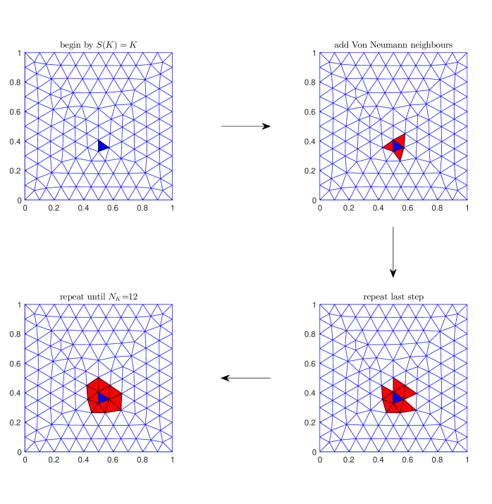
Figure 2.1. Build an element patch.

Let $U_{h}$ be the piecewise constant space associated with $\mathcal{T}_{h}$, i.e.,

$$U_{h}{:}=\{\,v\in L^{2}(\Omega)\,\mid\,v|_{K}\in\mathbb{P}_{0}(K),\ \text{for all\quad}K\in\mathcal{T}_{h}\},$$

where $\mathbb{P}_{r}$ is the polynomial space of degree not greater than $r$.

For any function $g\in U_{h}$, we reconstruct a polynomial $\mathcal{R}_{K}g$ of degree $m$ on $S(K)$ by solving the following least-squares:

(2.4) $$\mathcal{R}_{K}g=\operatorname{argmin}_{p\in\mathbb{P}_{m}(S(K))}\ \sum_{x\in\mathcal{I}_{K}}\left\lvert g(x)-p(x)\right\rvert^{2}.$$

The uniqueness condition for Problem (2.4) relates to the location of the collocation points and $\#S(K)$. Following [13, 12], we make the following assumption:

Assumption 2.1.

For all $K\in\mathcal{T}_{h}$ and $p\in\mathbb{P}_{m}(S(K))$,

(2.5) $$p|_{\mathcal{I}_{K}}=0\quad\text{implies\quad}p|_{S(K)}\equiv 0,$$

The above assumption guarantees the uniqueness of the solution of Problem (2.4) if $\#S(K)$ is greater than $\text{dim}\,\mathbb{P}_{m}$. Hereafter, we assume that this assumption is always valid.

From (2.4) we define the global reconstruction operator $\mathcal{R}$ for $g\in U_{h}$ by restricting the polynomial $\mathcal{R}_{K}g$ on $K$, $\mathcal{R}g|_{K}=(\mathcal{R}_{K}g)|_{K}$. Therefore, the operator $\mathcal{R}$ defines a map from $U_{h}$ to a discontinuous piecewise polynomial space with order $m$, which is denoted as $V_{h}=\mathcal{R}U_{h}$.

Next we investigate the behaviour of the basis functions, which are generated by the reconstruction process. Let $\boldsymbol{e}_{K}\in\mathbb{R}^{Ne}$, whose components are given by

$$e_{K,\widetilde{K}}=\delta_{K,\widetilde{K}},\quad\text{for all\quad}\widetilde{K}\in\mathcal{T}_{h},$$

where

$$\delta_{K,\widetilde{K}}=\begin{cases}1,\ K=\widetilde{K},\\ 0,\ K\neq\widetilde{K}.\\ \end{cases}$$

Then we denote $\{\lambda_{K}|\lambda_{K}=\mathcal{R}\boldsymbol{e}_{K}$ $\text{for all\quad}K\in\mathcal{T}_{h}\}$ as a group of basis functions. Given $\{\lambda_{K}\}$ we may write the reconstruction operator in an explicit way:

(2.6) $$\mathcal{R}g=\sum_{K\in\mathcal{T}_{h}}g(\boldsymbol{x}_{K})\lambda_{K}(\boldsymbol{x}),\quad\text{for all\quad}g\in U_{h}.$$

The operator $\mathcal{R}$ may be defined for continuous functions posed on $\Omega$ as (2.6) .

The support of $\lambda_{K}$ can be described as:

$$\text{supp}\lambda_{K}=\bigcup_{K^{\prime}\in S(K)}\overline{K^{\prime}}.$$

A one-dimensional example is presented in Section 4 and Figure 4.2.

It is worthwhile to mention that firstly the support of the basis function may not be equal to the element patch, and vice versus; secondly, the basis function is discontinuous, which lends itself ideally to the DG framework.

To state the method, we introduce some notations. Define the broken Sobolev spaces:

$$H^{s}(\Omega,\mathcal{T}_{h})=\{\,u\in L^{2}(\Omega)\,\mid\,u|_{K}\in H^{s}(K)\;\text{for all\;}K\in\mathcal{T}_{h}\},$$

where $H^{s}(K)$ is the standard Sobolev space on element $K$ associated with the norm $\|\cdot\|_{H^{s}(K)}$ and the seminorm $\left\lvert\cdot\right\rvert_{H^{s}(K)}$. The associated broken norm and seminorm are defined respectively by

$$\|\,u\,\|_{H^{s}(\Omega,\mathcal{T}_{h})}^{2}=\sum_{K\in\mathcal{T}_{h}}\|u\|_{H^{s}(K)}^{2},\quad\text{and}\quad\left\lvert u\right\rvert_{H^{s}(\Omega,\mathcal{T}_{h})}^{2}=\sum_{K\in\mathcal{T}_{h}}\left\lvert u\right\rvert_{H^{s}(K)}^{2}.$$

For two neighbouring elements $K^{+},K^{-}$ that share a common face $e=\partial K^{+}\cap\partial K^{-}$ with $e\in\mathcal{E}_{h}^{i}$, denote by $n^{+}$ and $n^{-}$ the outward unit normal vectors on $e$, corresponding to $\partial K^{+}$ and $\partial K^{-}$, respectively. For any function $q\in H^{1}(\Omega,\mathcal{T}_{h})$ and $v\in[H^{1}(\Omega,\mathcal{T}_{h})]^{d}$ that may be discontinuous across interelement boundaries, we define the average operator $\{\cdot\}$ and the jump operator $[[\cdot]]$ as

$$\{q\}=\frac{1}{2}(q^{+}+q^{-}),\quad\{v\}=\frac{1}{2}(v^{+}+v^{-}),$$

and

$$[\![q]\!]=n^{+}q^{+}+n^{-}q^{-},\quad[\![v]\!]=n^{+}\cdot v^{+}+n^{-}\cdot v^{-}.$$

Here $q^{+}=q|_{K^{+}},\ v^{+}=v|_{K^{+}}$ and $q^{-}=q|_{K^{-}},\ v^{-}=v|_{K^{-}}$. In the case $e\in\mathcal{E}_{h}^{b}$, there exists an element $K$ such that $e=K\cap\partial\Omega$, the definitions are changed to

$$\{q\}=q|_{K\cap\partial\Omega},\quad[\![q]\!]=nq|_{K\cap\partial\Omega},$$

and

$$\{v\}=v|_{K\cap\partial\Omega},\quad[\![v]\!]=n\cdot v|_{K\cap\partial\Omega}.$$

Following [4], for any $w\in H^{2}(\Omega,\mathcal{T}_{h})$, we define the energy norm $\|\,\cdot\,\|_{h}$ as

$$\|\,w\,\|_{h}^{2}=\sum_{K\in\mathcal{T}_{h}}\|\,\Delta w\,\|_{L^{2}(K)}^{2}+\|\,h_{e}^{-3/2}[\![w]\!]\,\|_{L^{2}(\mathcal{E}_{h})}^{2}+\|\,h_{e}^{-1/2}[\![\nabla w]\!]\,\|_{L^{2}(\mathcal{E}_{h})}^{2},$$

where

$$\|\,h_{e}^{-3/2}[\![w]\!]\,\|_{L^{2}(\mathcal{E}_{h})}^{2}{:}=\sum_{e\in\mathcal{E}_{h}^{i}}h_{e}^{-3}\|\,[\![w]\!]\,\|_{L^{2}(e)}^{2}\qquad\|\,h_{e}^{-1/2}[\![\nabla w]\!]\,\|_{L^{2}(\mathcal{E}_{h})}^{2}{:}=\sum_{e\in\mathcal{E}_{h}^{i}}h_{e}^{-1}\|\,[\![\nabla w]\!]\,\|_{L^{2}(e)}^{2}.$$

This energy norm $\|\,w\,\|_{h}$ is equivalent to $\|\,w\,\|_{H^{2}(\Omega,\mathcal{T}_{h})}$.

Next, we turn to the stability estimate of the reconstruction operator $\mathcal{R}$. By [13], we define $\Lambda(m,\mathcal{I}_{K})$ for any element $K\in\mathcal{T}_{h}$ as

(2.7) $$\Lambda(m,\mathcal{I}_{K})\triangleq\max_{p\in\mathbb{P}_{m}(S(K))}\frac{\max_{x\in S(K)}|p(\boldsymbol{x})|}{\max_{x\in\mathcal{I}_{K}}|p(x)|}.$$

By Assumption 2.1, we may conclude that $\Lambda(m,\mathcal{I}_{K})$ is finite. With some further conditions on $S(K)$, we conclude that $\Lambda(m,\mathcal{I}_{K})$ has a uniform upper bound, which is denoted by $\Lambda_{m}$. One of such condition may be found in the following lemma.

Lemma 2.1.

[13, Lemma 3.5] If each element patch $S(K)$ is convex and the triangulation is quasi-uniform, then $\Lambda_{m}$ is uniformly bounded.

The above condition is not necessary, we refer to [12] for the discussion on the uniform upper bound for non-convex element patch.

With the uniformly bounded $\Lambda_{m}$, we have the following quasi-optimal approximation estimates for the reconstruction operator in the maximum norm.

Lemma 2.2.

[13, Theorem 3.3] If Assumption 2.1 holds, the stability estimate holds true for any $K\in\mathcal{T}_{h}$ and $g\in C^{0}(S(K))$ as

(2.8) $$\|g-\mathcal{R}g\|_{L^{\infty}(K)}\leq C\Lambda_{m}\inf_{p\in\mathbb{P}_{m}(S(K))}\|g-p\|_{L^{\infty}(S(K))},$$

where $C$ is independent of $h$ but depends on $\#S(K)$.

The above lemma immediately implies the quasi-optimal approximation results in other norms.

Lemma 2.3.

Let $g\in H^{t}(\Omega)(t\geq 2)$ and $K\in\mathcal{T}_{h}$, there exists $C$ independent of $h$ but depends on $\#S(K)$ such that for $q=0,1,2$,

(2.9) $$\|g-\mathcal{R}g\|_{H^{q}(K)}\leq C\Lambda_{m}h^{s-q}\|g\|_{H^{t}(S(K),\mathcal{T}_{h})},$$

and for $q=1,2$

(2.10) $$\|\nabla^{q}(g-\mathcal{R}g)\|_{L^{2}(\partial K)}\leq C\Lambda_{m}h^{s-q-1/2}\|g\|_{H^{t}(S(K),\mathcal{T}_{h})}.$$

where $s=\min(m+1,t)$.

Proof.

By the standard interpolation estimate and (2.8), we obtain

$$\|g-\mathcal{R}g\|_{L^{2}(K)} \leq|K|^{1/2}\|g-\mathcal{R}_{m}g\|_{L^{\infty}(K)}$$

$$\leq C|K|^{1/2}\Lambda_{m}\inf_{p\in\mathbb{P}^{m}(S(K))}\|g-p\|_{L^{\infty}(S(K))}$$

$$\leq C\Lambda_{m}h^{s}\|g\|_{H^{t}(S(K),\mathcal{T}_{h})},$$

which gives (2.9) with $q=0$.

Let $g_{m}$ be the approximation polynomial in (2.2) for $g$, using (2.3), we obtain

$$\|\,\nabla(g-\mathcal{R}g)\,\|_{L^{2}(K)} \leq\|\,\nabla(g-g_{m})\,\|_{L^{2}(K)}+\|\,\nabla(g_{m}-\mathcal{R}g)\,\|_{L^{2}(K)}$$

$$\leq\|\,\nabla(g-g_{m})\,\|_{L^{2}(K)}+Ch_{K}^{-1}\|\,g_{m}-\mathcal{R}g\,\|_{L^{2}(K)}$$

$$\leq\|\,\nabla(g-g_{m})\,\|_{L^{2}(K)}+Ch_{K}^{-1}\|\,g-g_{m}\,\|_{L^{2}(K)}+Ch_{K}^{-1}\|\,g-\mathcal{R}g\,\|_{L^{2}(K)}$$

$$\leq Ch_{K}^{s}\|\,g\,\|_{H^{t}(S(K),\mathcal{T}_{h})},$$

which yields (2.9) with $q=1$ by using (2.9) with $q=0$ in the last step.

Proceeded along the same line that leads to (2.9) with $q=1$, we obtain (2.9) with $q=2$.

Using Agmon inequality (2.1) and (2.9), we obtain (2.10), which completes the proof. ∎

Using the above lemma, we obtain the following interpolation estimate for the reconstruction operator in the energy norm.

Theorem 2.1.

Let $g\in H^{t}(\Omega)$ with $t\geq 2$. There exists a constant $C$ independent of $h$ such that

(2.11) $$\|\,g-\mathcal{R}g\,\|_{h}\leq C\Lambda_{m}h^{s-2}\|g\|_{H^{t}(\Omega,\mathcal{T}_{h})},$$

where $s=\min(m+1,t)$.

3. Error Estimate for the Biharmonic Problem

Let us consider the biharmonic problem: find $u\in H^{4}(\Omega)$, such that

(3.1) $$\begin{cases}\Delta^{2}u=f,\quad&x\in\Omega,\\ u=g_{D},\quad&x\in\partial\Omega,\\ \partial_{n}u=g_{N},\quad&x\in\partial\Omega,\end{cases}$$

where $\Delta^{2}u=\Delta(\Delta u)$, $n$ denotes the unit outward normal vector to $\partial\Omega$, $f\in L^{2}(\Omega)$, $g_{D}$ and $g_{N}$ are assumed to be suitably smooth such that under proper conditions on $\Omega$, the boundary value problem (3.1) has a unique solution. We refer to [16] for precise description of such results.

The IPDG method [6] employs the following bilinear form $B$: for any $v,w\in H^{4}(\Omega,\mathcal{T}_{h})$,

$$B(v,w) =\sum_{K\in\mathcal{T}_{h}}\int_{K}\Delta v\Delta w\,\mathrm{d}x+\sum_{e\in\mathcal{E}_{h}}\int_{e}([\![v]\!]\cdot\{\nabla\Delta w\}+[\![w]\!]\cdot\{\nabla\Delta v\})\mathrm{d}s$$

$$\quad-\sum_{e\in\mathcal{E}_{h}}\int_{e}(\{\Delta w\}[\![\nabla v]\!]+\{\Delta v\}[\![\nabla w]\!])\mathrm{d}s+\sum_{e\in\mathcal{E}_{h}}\int_{e}\left(\alpha[\![v]\!][\![w]\!]+\beta[\![\nabla v]\!][\![\nabla w]\!]\right)\mathrm{d}s.$$

The piecewise penalty parameters $\alpha$ and $\beta$ are nonnegative and will be specified later on. The linear form $l$ is defined for all $v\in H^{4}(\Omega,\mathcal{T}_{h})$ as

$$l(v)=\int_{\Omega}fv\,\mathrm{d}x+\sum_{e\in\mathcal{E}_{h}^{b}}\int_{e}\left(g_{D}[\partial_{n}\Delta v+\alpha v]+g_{N}[\beta\partial_{n}v-\Delta v]\right)\mathrm{d}s.$$

The discretized problem is to find $u_{h}\in U_{h}$ such that for all $v_{h}\in U_{h}$,

(3.2) $$B(\mathcal{R}u_{h},\mathcal{R}v_{h})=l(\mathcal{R}v_{h}).$$

We begin the error estimate by defining the lifting operator $\mathcal{L}:H^{4}(\Omega,\mathcal{T}_{h})\rightarrow P_{h}$ [6]:

(3.3) $$\int_{\Omega}\mathcal{L}(w)r\,\mathrm{d}x=\int_{\mathcal{E}_{h}}([[w]]\cdot\{\nabla r\}-\{r\}[[\nabla w]])\mathrm{d}s\quad\text{for all\;}r\in P_{h},$$

where $P_{h}$ is defined by

$$P_{h}\triangleq\big{\{}w\in L^{2}(\Omega)\ \big{|}\ w|_{K}\in\mathbb{P}_{m}(K),\ \forall K\in\mathcal{T}_{h}\big{\}}.$$

The following lemma [6] gives the stability of the lifting operator.

Lemma 3.1.

For all $w\in H^{4}(\Omega,\mathcal{T}_{h})$, the following estimate holds:

$$\|\mathcal{L}(w)\|_{L^{2}(\Omega)}^{2}\leq\|\sqrt{\gamma}[[w]]\|_{L^{2}(\mathcal{E}_{h})}^{2}+\|\sqrt{\delta}[[\nabla w]]\|_{L^{2}(\mathcal{E}_{h})}^{2},$$

for piecewise constants $\gamma,\delta$ that are defined for all $e\in\mathcal{E}_{h}$ by

$$\gamma|_{e}=\frac{C_{\gamma}}{h_{e}^{3}},\quad\delta|_{e}=\frac{C_{\delta}}{h_{e}},\quad\text{for all\quad}e\in\mathcal{E}_{h},$$

with sufficiently large positive constants $C_{\gamma}$ and $C_{\delta}$.

With the definition of the DG energy norm and the Lemma 3.1, we show the bilinear form $B(\cdot,\cdot)$ satisfies the boundedness and the stability condition.

Lemma 3.2.

Let $\alpha,\beta>0$, there exists a positive constant $\Lambda$ which is independent of mesh size $h$ such that for all $v,w\in H^{4}(\Omega,\mathcal{T}_{h})$, there holds

(3.4) $$|B(v,w)|\leq\Lambda\|v\|_{h}\|w\|_{h}.\quad$$

Proof.

By the lifting operator (3.3), the bilinear form $B$ may be written as

(3.5) $$B(v,w)=\int_{\Omega}\big{(}\Delta v\Delta w +\mathcal{L}(v)\Delta w+\Delta v\mathcal{L}(w)\big{)}\,\mathrm{d}x$$

$$+\int_{\mathcal{E}_{h}}\big{(}\alpha[[v]][[w]]+\beta[[\nabla v]][[\nabla w]]\big{)}\mathrm{d}s.$$

Therefore, we obtain

$$|B(v,w)|\leq \|\Delta v\|_{L^{2}(\Omega)}\|\Delta w\|_{L^{2}(\Omega)}+\|\mathcal{L}(v)\|_{L^{2}(\Omega)}\|\Delta w\|_{L^{2}(\Omega)}$$

$$+\|\Delta v\|_{L^{2}(\Omega)}\|\mathcal{L}(w)\|_{L^{2}(\Omega)}+\|\sqrt{\alpha}[[v]]\|_{L^{2}(\Omega)}\|\sqrt{\alpha}[[w]]\|_{L^{2}(\mathcal{E}_{h})}$$

$$+\|\sqrt{\beta}[[\nabla v]]\|_{L^{2}(\mathcal{E}_{h})}\|\sqrt{\beta}[[\nabla w]]\|_{L^{2}(\mathcal{E}_{h})}$$

$$\leq \Lambda\|v\|_{h}\|w\|_{h}.$$

∎

Lemma 3.3.

Let

(3.6) $$\alpha|_{e}=\mu/h_{e}^{3}\quad\text{and\quad}\beta|_{e}=\eta/h_{e}$$

on $e\in\mathcal{E}_{h}$, where $\mu$ and $\eta$ are positive constants. With sufficiently large $\mu$ and $\eta$, there exists a positive constant $\lambda$ that is independent of mesh size $h$ such that for all $v_{h}\in U_{h}$

(3.7) $$B(\mathcal{R}v_{h},\mathcal{R}v_{h})\geq\lambda\|\mathcal{R}v_{h}\|_{h}^{2}.$$

Proof.

By the definition, we write

$$B(\mathcal{R}v_{h},\mathcal{R}v_{h}) =\|\Delta\mathcal{R}v_{h}\|_{L^{2}(\Omega)}^{2}+\|\sqrt{\alpha}[[\mathcal{R}v_{h}]]\|_{L^{2}(\mathcal{E}_{h})}^{2}+\|\sqrt{\beta}[[\nabla\mathcal{R}v_{h}]]\|_{L^{2}(\mathcal{E}_{h})}^{2}$$

$$\hskip 100.0pt+2\int_{\Omega}\mathcal{L}(\mathcal{R}v_{h})\Delta\mathcal{R}v_{h}\,\mathrm{d}x.$$

Using the inequality

$$-2\int_{\Omega}\mathcal{L}(\mathcal{R}v_{h})\Delta\mathcal{R}v_{h}\,\mathrm{d}x\leq 2\|\mathcal{L}(\mathcal{R}v_{h})\|_{L^{2}(\Omega)}^{2}+\frac{1}{2}\|\Delta\mathcal{R}v_{h}\|_{L^{2}(\Omega)}^{2},$$

and Lemma 3.1, we obtain

$$B(\mathcal{R}v_{h},\mathcal{R}v_{h})\geq\frac{1}{2}\|\Delta\mathcal{R}v_{h}\|_{L^{2}(\Omega)}^{2}+\|\sqrt{\alpha-4\gamma}[[\mathcal{R}v_{h}]]\|_{L^{2}(\mathcal{E}_{h})}^{2}+\|\sqrt{\beta-4\delta}[[\nabla\mathcal{R}v_{h}]]\|_{L^{2}(\mathcal{E}_{h})}^{2},$$

hence, the coercivity follows if $\alpha>4\gamma$ and $\beta>4\delta$. ∎

We are ready to prove a priori error estimates for Problem (3.2).

Theorem 3.1.

Let $u_{h}$ be the solution of Problem (3.2) and let the exact solution $u$ to the Problem (3.1) belong to the broken Sobolev space $H^{t}(\Omega,\mathcal{T}_{h})$ with $t\geq 4$. Furthermore, let the penalty functions $\alpha$ and $\beta$ satisfy the condition (3.6) in Lemma 3.7. Then

(3.8) $$\|\,u-\mathcal{R}u_{h}\,\|_{h}\leq Ch^{s-2}\|\,u\,\|_{H^{t}(\Omega,\mathcal{T}_{h})},$$

where $s=\min(m+1,t)$ and $s\geq 3$.

Proof.

We begin with the Galerkin orthogonality: for all $v_{h}\in U_{h}$, there holds

(3.9) $$B(u-\mathcal{R}u_{h},\mathcal{R}v_{h})=0.$$

Denote $w=\mathcal{R}u-\mathcal{R}u_{h}$, and using the above Galerkin orthogonality, we obtain

$$B(w,w)=B(\mathcal{R}u-u,w)+B(u-\mathcal{R}u_{h},w)=B(\mathcal{R}u-u,w).$$

Using (3.7) and (3.4), we obtain

$$\|\,\mathcal{R}u-\mathcal{R}u_{h}\,\|_{h}\leq\dfrac{\Lambda}{\lambda}\|\,u-\mathcal{R}u\,\|_{h}.$$

By the triangle inequality we immediately obtain

$$\|\,u-\mathcal{R}u_{h}\,\|_{h}\leq(1+\Lambda/\lambda)\|\,u-\mathcal{R}u\,\|_{h},$$

which together with (2.11) gives the estimate (3.8). ∎

The $L^{2}$ error estimate may be obtained by standard duality argument. Following [5], we make the regularity assumptions: the solution $\psi$ of problem

(3.10) $$\left\{\begin{aligned} \Delta^{2}\psi&=u-\mathcal{R}u_{h},\quad&&\text{in}\quad\Omega,\\ \psi=\dfrac{\partial\psi}{\partial n}&=0,\quad&&\text{on\quad}\partial\Omega,\end{aligned}\right.$$

belongs to $H^{4}(\Omega)$, and there exists a positive constant $C$ that only depends on $\Omega$ such that

(3.11) $$\|\psi\|_{H^{4}(\Omega)}\leq C\|u-\mathcal{R}u_{h}\|_{L^{2}(\Omega)}.$$

Theorem 3.2.

Besides the conditions in Theorem 3.1, we assume the elliptic regularity (3.11) holds true, then

(3.12) $$\|u-\mathcal{R}u_{h}\|_{L^{2}(\Omega)} \leq Ch^{2}\|u\|_{H^{t}(\Omega,\mathcal{T}_{h})},\quad m=2,$$

(3.13) $$\|u-\mathcal{R}u_{h}\|_{L^{2}(\Omega)} \leq Ch^{s}\|u\|_{H^{t}(\Omega,\mathcal{T}_{h})},\quad m\geq 3,$$

where $s=\min(m+1,t)$.

Proof.

An integration by parts gives

$$\|u-\mathcal{R}u_{h}\|_{L^{2}(\Omega)}^{2}=B(\psi,u-\mathcal{R}u_{h})=B(\psi-\mathcal{R}\psi,u-\mathcal{R}u_{h}),$$

where we have used the Galerkin orthogonality in the last step. Combining the interpolation estimate, the energy estimate (3.8) and the regularity estimate (3.11) gives (3.12) and (3.13). ∎

4. Implementation and Numerical Results

In this section, we describe the implementation details of the reconstructed space and report some numerical examples to show the accuracy and performance of the proposed method. In all examples, we build element patches by the first method and use a sparse direct solver for the resulting sparse linear systems.

4.1. Implementation

The key point of the implementation is to calculate the basis functions and here we present a one-dimensional example on the interval $[0,1]$. Consider a uniform mesh consisting of $5$ elements $\{K_{1},K_{2},K_{3},K_{4},K_{5}\}$; see Figure 4.1.

Figure 4.1. The uniform mesh on $[0,1]$.

We choose the midpoint of each element as the collocation point to reconstruct a piecewise linear space. The element patches are taken as

$$S(K_{1}) =\{K_{1},K_{2},K_{3}\},\quad S(K_{i})=\{K_{i-1},K_{i},K_{i+1}\},\ i=2,3,4,$$

$$S(K_{5}) =\{K_{3},K_{4},K_{5}\}.$$

The local least-squares (2.4) on element $K_{i}$ is

$$\mathcal{R}_{K_{i}}g=\operatorname{argmin}_{\{a,b\}\in\mathbb{R}}\ \sum_{x_{K^{\prime}}\in\mathcal{I}_{K_{i}}}\left\lvert g(x_{K^{\prime}})-(ax_{K^{\prime}}+b)\right\rvert^{2}.$$

A direct calculation gives

$$[a,b]^{T}=(A^{T}A)^{-1}A^{T}q,$$

where $A$ and $q$ are given as follows. For $i=1$,

$$A=\begin{bmatrix}1&x_{K_{1}}\\ 1&x_{K_{2}}\\ 1&x_{K_{3}}\end{bmatrix},\quad q=\begin{bmatrix}g(x_{K_{1}})\\ g(x_{K_{2}})\\ g(x_{K_{3}})\end{bmatrix},$$

and for $i=2,3,4$,

$$A=\begin{bmatrix}1&x_{K_{i-1}}\\ 1&x_{K_{i}}\\ 1&x_{K_{i+1}}\end{bmatrix},\quad q=\begin{bmatrix}g(x_{K_{i-1}})\\ g(x_{K_{i}})\\ g(x_{K_{i+1}})\end{bmatrix},$$

and for $i=5$,

$$A=\begin{bmatrix}1&x_{K_{3}}\\ 1&x_{K_{4}}\\ 1&x_{K_{5}}\end{bmatrix}\quad q=\begin{bmatrix}g(x_{K_{3}})\\ g(x_{K_{4}})\\ g(x_{K_{5}})\end{bmatrix}.$$

The basis functions $\{\lambda_{K}\}$ are plot in Figure 4.2.

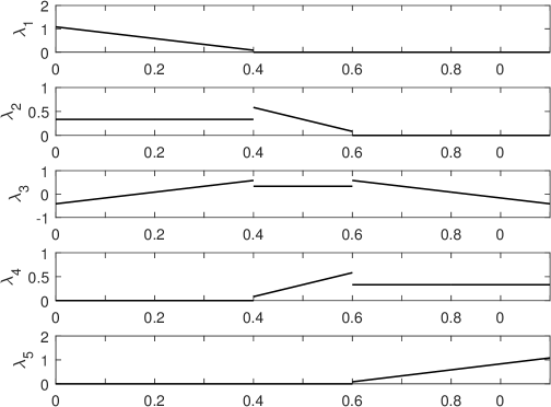
Figure 4.2. The basis functions.

Thus we store $(A^{T}A)^{-1}A^{T}$ for each element to represent the basis functions and it is the same when we deal with the high dimensional problem.

4.2. 2D Smooth Solutions

We firstly study the convergence rate for smooth solutions of two-dimensional problems.

Table 4.1. uniform $\#S(K)$ for 2D smooth solutions

polynomial degree $m$		2	3	4	5	6
$\#S(K)$	Example 1	9	15	22	29	38
	Example 2	9	16	23	32	45
	Example 3	9	20	28	38	49

Example 1. Consider the biharmonic problem on the domain $\Omega=(0,1)^{2}$ with Dirichlet boundary condition. The exact solution is taken as

(4.1) $$u(x,y)=\sin^{2}(\pi x)\sin^{2}(\pi y),\quad(x,y)\in\Omega,$$

and $g_{D}$, $g_{N}$ and the source term $f$ are chosen accordingly. The polynomial degree $m$ is taken by $m=2,\cdots,6$. And the domain $\Omega$ is partitioned into several regular disjoint elements for each mesh size $h$; see Figure 4.3, where $h=1/10,1/20,1/40$ and $h=1/80$. We choose $\#S(K)$ uniformly for all elements as in the second row of Table 4.1.

In Figure 4.4, we present the errors measured in both the DG norm and the $L^{2}$ norm. It is clear that the convergence rate in the DG norm is $m-1$ for fixed $m$. The convergence rate in the L² norm is $m+1$ for $m\geq 3$, which converges quadratically when $m=2$. Such convergence rate is consistent with the theoretical prediction in Theorem 3.1.

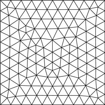
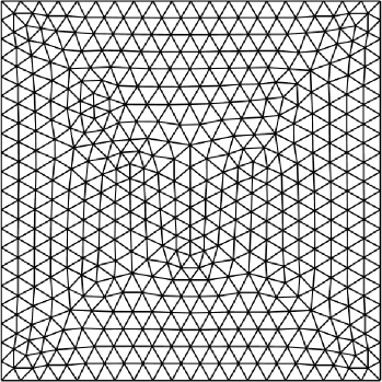
Figure 4.3. The triangular meshes for Example 1.

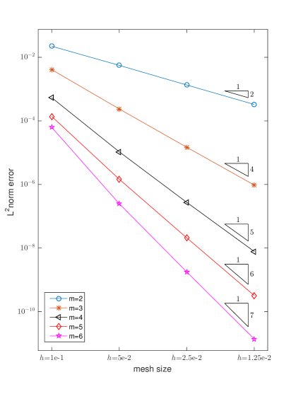
Figure 4.4. Examples 1: The convergence rate in the L² norm (left) and the DG norm (right) for different $m$ on triangular meshes.

Example 2. As we emphasize before, the local least-squares problem (2.4) is independent of the element geometry. In this example, we use the mesh generator in [17] to obtain a series of polygonal meshes from the Voronoi diagram of a given set of their reflections; see Figure 4.5. We also take (4.1) as the exact solution. The number $\#S(K)$ is chosen as in the third row of Table 4.1.

For each fixed $m$, we present the errors in both the DG norm and the $L^{2}$ norm against the number of elements; see Figure 4.6. It is clear that the numerical results still agree well with the theoretical results.

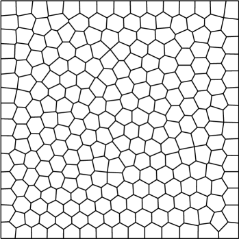
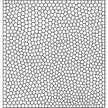
Figure 4.5. The Voronoi meshes for Example 2.

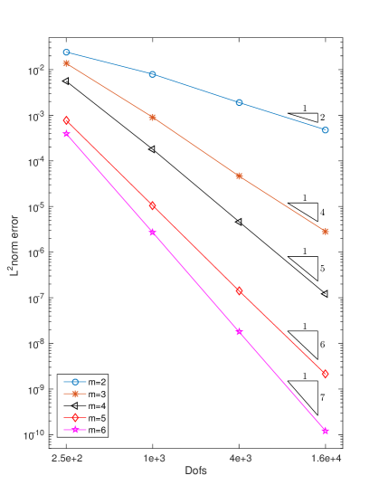
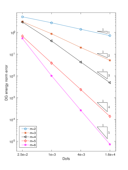
Figure 4.6. Examples 2: The convergence rate in the L² norm (left) and the DG energy norm (right) for different $m$ on Voronoi meshes.

Example 3. In this test, we consider the biharmonic problem on $\Omega=(0,1)^{2}$ with the following boundary condition [18]:

$$u=\Delta u=0,\quad x\in\partial\Omega,$$

which is related to the bending of a simply supported plate. We take $u(x,y)=\sin(2\pi x)\sin(2\pi y)$ as the exact solution. The mesh consists of a mixing of triangular and quadrilateral elements, which are generated by gmsh[19]; see Figure 4.7. The mesh size $h$ varies equally from $1/10$ to $h=1/80$. We take $\#S(K)$ as in the last row of Table 4.1. The results in Figure 4.8 show the convergence rate for different $m$, which are also consistent with the theoretical results.

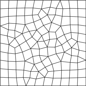
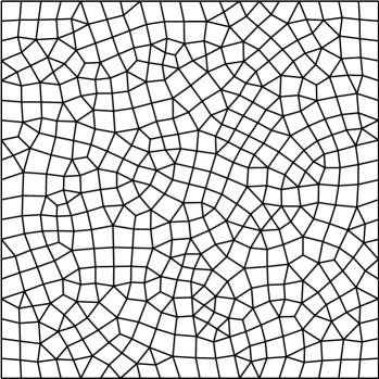
Figure 4.7. The mixed meshes for Example 3.

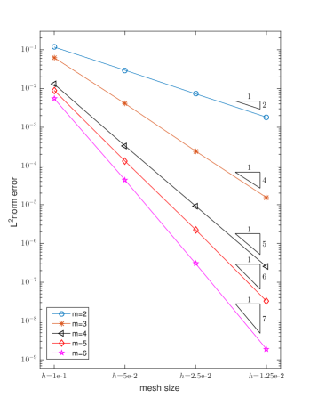
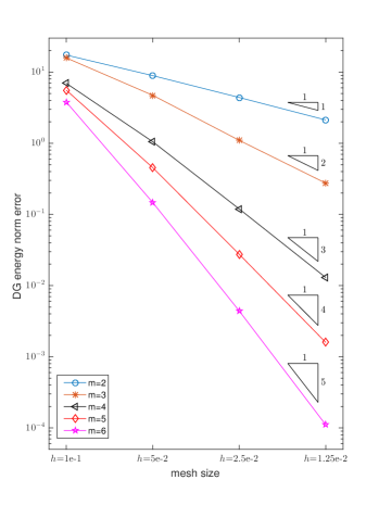
Figure 4.8. Examples 3: The convergence rate in the L² norm (left) and the DG energy norm (right) for different $m$ on mixed meshes.

Example 4. In this test, we compare the $C^{0}$IPG, IPDG and the proposed method by solving the biharmonic problem in the domain $\Omega=(0,1)^{2}$ with the same exact solution as for Example 1. The meshes used for this case are obtained by successively refining an initial mesh with $h=0.2$. We measure the errors in both the broken $H^{2}$ norm and the $L^{2}$ norm. Figure 4.9 and Figure 4.10 show the performance of three methods by using spaces of polynomials of degree 2 and 3, respectively. We plot the errors in both norms against the number of degrees of freedom. It is clear that the proposed method behaves slightly better than other methods.

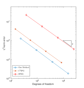
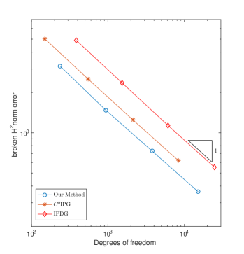
Figure 4.9. The error in $\|\cdot\|_{L^{2}(\Omega)}$ (left)/ $\|\cdot\|_{H^{2}(\Omega,\mathcal{T}_{h})}$ (right) for three methods by using second order polynomials.

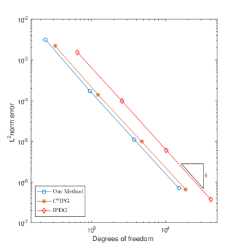
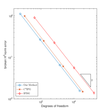
Figure 4.10. The error in $\|\cdot\|_{L^{2}(\Omega)}$ (left)/ $\|\cdot\|_{H^{2}(\Omega,\mathcal{T}_{h})}$ (right) for three methods by using third order polynomials.

4.3. L-shaped domain with known exact solution

In this example, we study the performance of the proposed method with the problem with a corner singularity. Let $\Omega$ be the L-shaped domain $(-1,1)^{2}\backslash[0,1)\times(-1,0]$ and we use triangular meshes; see Figure 4.11. Following [6], we let

$$u(r,\theta)=r^{5/3}\sin(5\theta/3)$$

in polar coordinate and impose Dirichlet boundary condition. At the corner $(0,0)$ the exact solution contains a singularity which indicates $u$ only belongs to $H^{8/3-\epsilon}(\Omega)$ for $\epsilon>0$. The number $\#S(K)$ is chosen as in the second row of Table 4.1.

In Table 4.2, we list the error measured in the DG norm and the $L^{2}$ norm against the mesh size for $m=2,3,4$. Here we observe that the error in $L^{2}$ norm decreases at the rate $\mathcal{O}(h^{1.2})$ while the error in DG norm decreases at the rate $\mathcal{O}(h^{2/3})$. It seems the convergence rates agree with that in [6].

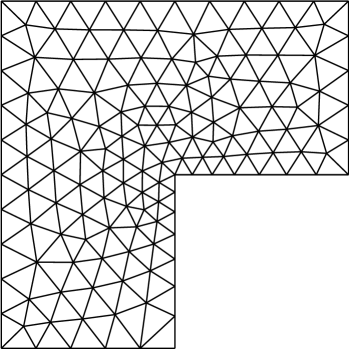
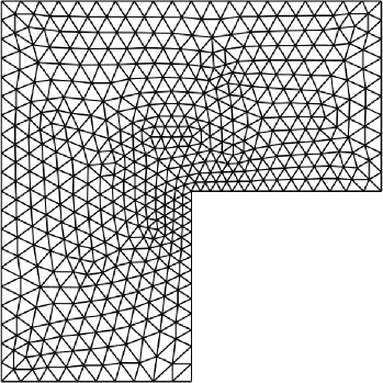
Figure 4.11. The triangular meshes of L-shaped domain

Table 4.2. Convergence rates of L-shaped domain example

$m$	Norm	Dofs	Dofs	Order	Dofs	Order	Dofs	Order	Dofs	Order
		$250$	$1000$		$4000$		$16000$		$64000$
		Error	Error		Error		Error		Error
2	$\|\cdot\|_{L^{2}(\Omega)}$	$1.38\mathrm{e}$-3	$6.15\mathrm{e}$-4	1.17	$2.68\mathrm{e}$-4	1.23	$1.17\mathrm{e}$-4	1.20	$5.13\mathrm{e}$-5	1.19
	$\|\cdot\|_{h}$	$3.35\mathrm{e}$-1	$2.03\mathrm{e}$-1	0.72	$1.23\mathrm{e}$-1	0.72	$7.63\mathrm{e}$-2	0.69	$4.73\mathrm{e}$-2	0.68
3	$\|\cdot\|_{L^{2}(\Omega)}$	$8.58\mathrm{e}$-4	$3.11\mathrm{e}$-4	1.47	$1.22\mathrm{e}$-4	1.35	$5.33\mathrm{e}$-5	1.19	$2.99\mathrm{e}$-5	1.21
	$\|\cdot\|_{h}$	$2.42\mathrm{e}$-1	$1.31\mathrm{e}$-1	0.88	$8.43\mathrm{e}$-1	0.64	$5.33\mathrm{e}$-2	0.66	$3.37\mathrm{e}$-2	0.66
4	$\|\cdot\|_{L^{2}(\Omega)}$	$1.08\mathrm{e}$-3	$3.19\mathrm{e}$-4	1.76	$1.11\mathrm{e}$-4	1.52	$4.56\mathrm{e}$-5	1.28	$1.95\mathrm{e}$-5	1.22
	$\|\cdot\|_{h}$	$3.43\mathrm{e}$-1	$1.76\mathrm{e}$-1	0.96	$1.08\mathrm{e}$-1	0.71	$6.78\mathrm{e}$-2	0.67	$4.25\mathrm{e}$-2	0.67

4.4. 3D Smooth Solution

In this example, we solve a three-dimensional biharmonic problem on a unit cube $\Omega=(0,1)^{3}$. The domain is partitioned into tetrahedral meshes with mesh size $h=1/4,1/8,1/16$ and $h=1/32$ by gmsh. The exact solution is chosen as $u(x,y,z)=\sin^{2}(\pi x)\sin^{2}(\pi y)\sin^{2}(\pi z)$ and the function $g_{D},g_{N}$ and $f$ are taken suitably. We build the reconstruction operator with different polynomial degrees $m=2,3,4$. The number $\#S(K)$ is listed in Table 4.3.

Table 4.3. Uniform $\#S(K)$ for 3D smooth solution

polynomial degree $m$	2	3	4
all $\#S(K)$	21	40	62

The numerical results are presented in Table 4.4. The convergence rates also agree with the theoretical prediction.

Table 4.4. Convergence rates of 3D example

m	Norm	Dofs	Dofs	Order	Dofs	Order	Dofs	Order
		384	3072		24576		196608
		Error	Error		Error		Error
2	$\|\cdot\|_{L^{2}(\Omega)}$	$7.34\mathrm{e}$-2	$1.43\mathrm{e}$-2	2.36	$3.34\mathrm{e}$-3	2.10	$8.07\mathrm{e}$-3	2.05
	$\|\cdot\|_{h}$	$8.87\mathrm{e}$-0	$4.59\mathrm{e}$-0	0.95	$2.41\mathrm{e}$-0	0.93	$1.22\mathrm{e}$-0	0.98
3	$\|\cdot\|_{L^{2}(\Omega)}$	$3.34\mathrm{e}$-2	$3.76\mathrm{e}$-3	3.15	$2.50\mathrm{e}$-4	3.91	$1.59\mathrm{e}$-5	3.97
	$\|\cdot\|_{h}$	$6.89\mathrm{e}$-0	$2.19\mathrm{e}$-0	1.66	$5.86\mathrm{e}$-1	1.90	$1.50\mathrm{e}$-1	1.97
4	$\|\cdot\|_{L^{2}(\Omega)}$	$2.83\mathrm{e}$-2	$8.96\mathrm{e}$-4	4.98	$2.43\mathrm{e}$-5	5.19	$7.11\mathrm{e}$-7	5.09
	$\|\cdot\|_{h}$	$5.09\mathrm{e}$-0	$1.03\mathrm{e}$-0	2.31	$1.42\mathrm{e}$-1	2.86	$1.68\mathrm{e}$-2	3.08

5. Conclusion

We propose a new discontinuous Galerkin method to solve the biharmonic boundary value problem. A novelty of the method is a new discontinuous polynomial space that is reconstructed by solving local least-squares. The optimal error estimates in both the DG energy norm and the $L^{2}$ norm are proved, which are confirmed by a series of numerical examples with different complexity.

References

- [1] O.C. Zienkiewicz, R.L. Taylor and D.D. Fox, The Finite Element Method for Solid and Structural Mechanics, Elsevier/Butterworth Heinemann, Amsterdam, seventh edition, 2014.
- [2] P. Hansbo and M.G. Larson, A discontinuous Galerkin method for the plate equation, Calcolo, 39:1 (2002), 41–59.
- [3] I. Mozolevski and E. Süli, A priori error analysis for the -version of the discontinuous Galerkin finite element method for the biharmonic equation, Comput. Methods Appl. Math., 3:4 (2003), 596–607.
- [4] E. Süli and I. Mozolevski, -version interior penalty DGFEMs for the biharmonic equation, Comput. Methods Appl. Mech. Engrg., 196:13-16 (2007), 1851–1863.
- [5] I. Mozolevski, E. Süli and P.R. Bösing, -version a priori error analysis of interior penalty discontinuous Galerkin finite element approximations to the biharmonic equation, J. Sci. Comput., 30:3 (2007), 465–491.
- [6] E.H. Georgoulis and P. Houston, Discontinuous Galerkin methods for the biharmonic problem, IMA J. Numer. Anal., 29:3 (2009), 573–594.
- [7] B. Cockburn, B. Dong and J. Guzmán, A hybridizable and superconvergent discontinuous Galerkin method for biharmonic problems, J. Sci. Comput., 40:1-3 (2009), 141–187.
- [8] T.J.R. Hughes, G. Engel, L. Mazzei and M.G. Larson, A comparison of discontinuous and continuous Galerkin methods based on error estimates, conservation, robustness and efficiency, Discontinuous Galerkin methods (Newport, RI, 1999), volume 11 of Lect. Notes Comput. Sci. Eng., pages 135–146, Springer, Berlin, 2000.
- [9] O.C. Zienkiewicz, R.L. Taylor, S.J. Sherwin and J. Peiró, On discontinuous Galerkin methods, Internat. J. Numer. Methods Engrg., 58:8 (2003), 1119–1148.
- [10] G. Engel, K. Garikipati, T.J.R. Hughes, M.G. Larson, L. Mazzei and R.L. Taylor, Continuous/discontinuous finite element approximations of fourth-order elliptic problems in structural and continuum mechanics with applications to thin beams and plates, and strain gradient elasticity, Comput. Methods Appl. Mech. Engrg., 191:34 (2002), 3669–3750.
- [11] S.C. Brenner, interior penalty methods, Frontiers in Numerical Analysis—Durham 2010, volume 85 of Lect. Notes Comput. Sci. Eng., pages 79–147, Springer, Heidelberg, 2012.
- [12] R. Li, P.B. Ming, Z.Y. Sun and Z.J. Yang, An arbitrary-order discontinuous Galerkin method with one unknown per element, arXiv:1803.00378, (2018).
- [13] R. Li, P.B. Ming and F. Tang, An efficient high order heterogeneous multiscale method for elliptic problems, Multiscale Model. Simul., 10:1 (2012), 259–283.
- [14] P.F. Antonietti, L.Beirão da Veiga and M. Verani, A mimetic discretization of elliptic obstacle problems, Math. Comp., 82:283 (2013), 1379–1400.
- [15] F. Brezzi, K. Lipnikov and V. Simoncini, A family of mimetic finite difference methods on polygonal and polyhedral meshes, Math. Models Methods Appl. Sci., 15:10 (2005), 1533–1551.
- [16] H. Blum and R. Rannacher, On the boundary value problem of the biharmonic operator on domains with angular corners, Math. Methods Appl. Sci., 2:4 (1980), 556–581.
- [17] C. Talischi, G.H. Paulino, A. Pereira and I.F.M. Menezes, PolyMesher: a general-purpose mesh generator for polygonal elements written in Matlab, Struct. Multidiscip. Optim., 45:3 (2012), 309–328.
- [18] S.C. Brenner, P. Monk and J. Sun, interior penalty Galerkin method for biharmonic eigenvalue problems, Spectral and High Order Methods for Partial Differential Equations—ICOSAHOM 2014, volume 106 of Lect. Notes Comput. Sci. Eng., pages 3–15, Springer, Cham, 2015.
- [19] C. Geuzaine and J.F. Remacle, Gmsh: A 3-D finite element mesh generator with built-in pre- and post-processing facilities, Internat. J. Numer. Methods Engrg., 79:11 (2009), 1309–1331.