Finite-Sample Bounds for the Multivariate Behrens–Fisher Distribution with Proportional Covariances

Abstract

The Behrens–Fisher problem is a well-known hypothesis testing problem in statistics concerning two-sample mean comparison. In this article, we confirm one conjecture in Eaton & Olshen (1972), which provides stochastic bounds for the multivariate Behrens–Fisher test statistic under the null hypothesis. We also extend their results on the stochastic ordering of random quotients to the arbitrary finite dimensional case. This work can also be seen as a generalization of Hsu (1938) that provided the bounds for the univariate Behrens–Fisher problem. The results obtained in this article can be used to derive a testing procedure for the multivariate Behrens–Fisher problem that strongly controls the Type I error.

Keywords: Behrens–Fisher problem; Hypothesis testing; Mean comparison; Stochastic bound; Type I error.

Department of Statistics, Purdue University, West Lafayette, Indiana 47907, U.S.A.

1 Introduction

The Behrens–Fisher problem is one of the most well-known hypothesis testing problems that has been extensively studied by many statisticians, partly due to its simple form and numerous real applications. The univariate Behrens–Fisher problem can be phrased as follows: Let $X=(X_{1},\ldots,X_{m})$ and $Y=(Y_{1},\ldots,Y_{n})$ be two independent random samples with $X_{i}\overset{iid}{\sim}N(\mu_{1},\sigma_{1}^{2})$ and $Y_{i}\overset{iid}{\sim}N(\mu_{2},\sigma_{2}^{2})$, where all the four parameters are unknown, and the target is to test $H_{0}:\mu_{1}=\mu_{2}$ versus $H_{a}:\mu_{1}\neq\mu_{2}$.

There was enormous research on designing a procedure to test this hypothesis, for example Fisher’s fiducial inference (Fisher, 1935), Scheffé’s $t$-distribution method (Scheffé, 1943), the generalized $p$-value method (Tsui & Weerahandi, 1989), the marginal inferential models (Martin & Liu, 2015), and many others that were summarized in review articles such as Scheffé (1970) and Kim & Cohen (1998). Among all these approaches, the most broadly-adopted test statistic is the Behrens–Fisher statistic. Using conventional notations, $\overline{X}$ and $\overline{Y}$ are the two sample means, $S_{1}^{2}$ and $S_{2}^{2}$ are the two unbiased sample variances, and then the Behrens–Fisher statistic is defined by $T=\left(S_{1}^{2}/m+S_{2}^{2}/n\right)^{-1/2}(\overline{X}-\overline{Y})$. It is well known that the sampling distribution of $T$ under $H_{0}$ depends on the unknown variance ratio $\sigma_{1}^{2}/\sigma_{2}^{2}$, and various methods were proposed to approximate this null distribution, for example the most widely-used Welch-Satterthwaite approximate degrees of freedom (Satterthwaite, 1946; Welch, 1947).

Despite their extreme popularity in applications, one critical issue of the approximation methods is that they do not guarantee the control of Type I error. Therefore, conservative test procedures that can strongly control the Type I error are also of interest. The remarkable works Hsu (1938) and Mickey & Brown (1966) showed that the distribution function of $T$ is bounded below by $t_{\min\{m-1,n-1\}}$, the $t$-distribution with $\min\{m-1,n-1\}$ degrees of freedom, and bounded above by $t_{m+n-2}$. With this result, one can use critical values or $p$-values based on $t_{\min\{m-1,n-1\}}$ to test the hypothesis, which ensures the limit of Type I error. This approach also motivated works such as Hayter (2013) and Martin & Liu (2015).

The Behrens–Fisher problem was also generalized to the multivariate case in various research articles. In this setting, each observation follows a multivariate normal distribution, and the target is to test the equality of the two mean vectors. In the multivariate case, most of the approaches are based on the approximate degrees of freedom framework, for example Yao (1965), Johansen (1980), Nel & Van der Merwe (1986), and Krishnamoorthy & Yu (2004). Also see Christensen & Rencher (1997) for a comparison of other solutions.

Alternatively, along the direction of Hsu (1938) and Mickey & Brown (1966), Eaton & Olshen (1972) attempted to develop stochastic bounds for the test statistic in the multivariate case, and they provided the result for the two-dimensional case with proportional covariances assumption. However, the theorem that they developed to prove the result had the restriction that it only applied to the two-dimensional case, so they left the general finite dimensional case as a conjecture.

In this article, we study the same problem as in Eaton & Olshen (1972) using a related but different approach, and we are able to confirm this conjecture and generalize their result to the arbitrary finite dimensional case. As a result, we provide sharp bounds for the multivariate Behrens–Fisher distribution with proportional covariances, as a direct generalization of Hsu’s result in the univariate case.

The remaining part of this article is organized as follows. In Section 2 we briefly introduce the multivariate Behrens–Fisher problem and review some existing results on it. Section 3 is the main part of this article, where two major theorems that describe the stochastic bounds for the test statistic are provided. In Section 4 we use numerical simulations to illustrate the performance of the proposed test compared with other approximation methods. And finally in Section 5, some discussions and the conclusion of this article are provided. The proofs of two important lemmas are in the appendix.

2 Multivariate Behrens–Fisher Problem

In this section we briefly describe the multivariate Behrens–Fisher problem and review some relevant results on it. Similar to the univariate case, let $X=(X_{1},\ldots,X_{m})^{\mathrm{T}}$ and $Y=(Y_{1},\ldots,Y_{n})^{\mathrm{T}}$ be two independent random samples, with each observation following a $p$-dimensional multivariate normal distribution: $X_{i}\overset{iid}{\sim}N(\mu_{1},\Sigma_{1})$, and $Y_{i}\overset{iid}{\sim}N(\mu_{2},\Sigma_{2})$. The problem of interest is to test $H_{0}:\mu_{1}=\mu_{2}$ versus $H_{a}:\mu_{1}\neq\mu_{2}$, with all the distributional parameters unknown. Following the same assumption in Eaton & Olshen (1972), we assume that $X$ and $Y$ have proportional covariances, i.e.,

$$\Sigma_{1}=\Sigma,\quad\Sigma_{2}=k\Sigma$$ (1)

for some unknown $p\times p$ positive definite matrix $\Sigma$ and an unknown constant $k$ ($k>0$). In the remaining part of this article we assume that $p<\min\{m,n\}$.

Let $\overline{X}=m^{-1}\sum_{i=1}^{m}X_{i}$ and $\overline{Y}=n^{-1}\sum_{i=1}^{n}Y_{i}$ be the sample means, and $S_{1}=(m-1)^{-1}\sum_{i=1}^{m}(X_{i}-\overline{X})(X_{i}-\overline{X})^{\mathrm{T}}$ and $S_{2}=(n-1)^{-1}\sum_{i=1}^{n}(Y_{i}-\overline{Y})(Y_{i}-\overline{Y})^{\mathrm{T}}$ be the sample covariance matrices. It is well known that $\overline{X}\sim N(\mu_{1},m^{-1}\Sigma_{1}),\overline{Y}\sim N(\mu_{2},n^{-1}\Sigma_{2}),(m-1)S_{1}\sim W(\Sigma_{1},m-1)$, and $(n-1)S_{2}\sim W(\Sigma_{2},n-1)$, where $W(\Sigma,n)$ stands for a Wishart distribution with parameter $\Sigma$ and $n$ degrees of freedom. All these four random vectors and matrices are independent of each other. Furthermore, the multivariate Behrens–Fisher test statistic is defined as

$$T^{2}=(\overline{X}-\overline{Y})^{\mathrm{T}}\left(m^{-1}S_{1}+n^{-1}S_{2}\right)^{-1}(\overline{X}-\overline{Y}),$$ (2)

and the sampling distribution of $T^{2}$ under $H_{0}$ is typically called the multivariate Behrens–Fisher distribution. In this article, our primary goal is to derive stochastic bounds for $T^{2}$ that are free of the unknown parameters.

A major progress on this direction was made by Eaton & Olshen (1972). They first showed that under $H_{0}$,

$$T^{2}\overset{d}{=}Z^{\mathrm{T}}\left\{\lambda(m-1)^{-1}W_{1}+(1-\lambda)(n-1)^{-1}W_{2}\right\}^{-1}Z,$$ (3)

where $X\overset{d}{=}Y$ means $X$ and $Y$ have the same distribution, $Z\sim N(0,I_{p}),W_{1}\sim W(I_{p},m-1),W_{2}\sim W(I_{p},n-1),\lambda=m^{-1}(m^{-1}+kn^{-1})^{-1}$, $I_{p}$ is the $p\times p$ identity matrix, and $Z,W_{1}$, and $W_{2}$ are independent. Then they proved that for $p=2$,

$$Z^{\mathrm{T}}\left\{(m+n-2)^{-1}W_{(m+n-2)}\right\}^{-1}Z\preceq_{st}T^{2}\preceq_{st}Z^{\mathrm{T}}\left\{\nu^{-1}W_{(\nu)}\right\}^{-1}Z,$$ (4)

where $\preceq_{st}$ stands for the stochastic ordering, $\nu$ is any integer satisfying $p\leq\nu\leq\min\{m-1,n-1\}$, and $W_{(n)}$ stands for a $W(I_{p},n)$ random matrix that is independent of $Z$.

However, in Eaton & Olshen (1972), (4) was only proved for the case of $p=2$, since the underlying theory did not generalize to higher dimensions. To overcome this difficulty, in this article we use a different set of techniques to prove that (4) also holds for $p>2$. The main results are presented in Section 3.

3 Main Results

We first present two lemmas that are the keys to our main theorems, whose proofs are given in the appendix. Lemma 1 studies the property of a linear combination of $Z_{i}^{2}$ random variables, where $Z_{i}\overset{iid}{\sim}N(0,1)$.

Lemma 1.

Assume that $Z_{1},\ldots,Z_{p}$ are $p$ independent $N(0,1)$ random variables. Let $F(t;\theta)=F(t;\theta_{1},\ldots,\theta_{p})$ denote the distribution function of the random variable $T_{\theta}=\sum_{i=1}^{p}Z_{i}^{2}/\theta_{i},\theta_{i}>0$, and define its partial derivatives as $f_{i}(t;\theta)=\partial F(t;\theta)/\partial\theta_{i}$ and $g_{i}(t;\theta)=\partial^{2}F(t;\theta)/\partial\theta_{i}^{2}$. Then for $i,j=1,\ldots,p$, we have

1. $f_{i}(t;\theta)>0$,

2. $g_{i}(t;\theta)<0$, and

3. If $\theta_{i}<\theta_{j}$ then $f_{i}(t;\theta)>f_{j}(t;\theta)$.

Lemma 1 itself gives some general properties of the distribution family represented by $T_{\theta}$, and in this article the lemma is mainly used to show the conclusion below, which is the central technical tool to prove our main theorems.

Lemma 2.

Assume that $Z$ is a $N(0,I_{p})$ random vector. Fix $t>0$ and let $M_{1}$ and $M_{2}$ be two $p\times p$ positive definite matrices. Define $h(\lambda;t,M_{1},M_{2})=\mathrm{pr}\left[Z^{\mathrm{T}}\left\{\lambda M_{1}+(1-\lambda)M_{2}\right\}^{-1}Z\leq t\right]$, and then $\partial^{2}h(\lambda;t,M_{1},M_{2})/\partial\lambda^{2}<0$.

To present the main theorems of this article, we first introduce two useful concepts: the majorization of vectors (Olkin & Marshall, 2016), and the exchangeability of a sequence of random vectors.

Definition 1.

Let $x=(x_{1},\ldots,x_{n})$ and $y=(y_{1},\ldots,y_{n})$ be two vectors in $\mathbb{R}^{n}$, and let $x_{[1]}\geq\cdots\geq x_{[n]}$ and $y_{[1]}\geq\cdots\geq y_{[n]}$ be the decreasing rearrangement of $x$ and $y$ respectively. $x$ is said to be majorized by $y$, denoted by $x\prec_{m}y$, if

$$\sum_{i=1}^{n}x_{[i]}=\sum_{i=1}^{n}y_{[i]}\text{ and }\sum_{i=1}^{k}x_{[i]}\leq\sum_{i=1}^{k}y_{[i]},k=1,2,\ldots,n-1.$$

Intuitively, $x\prec_{m}y$ indicates that $x$ and $y$ have the same total quantity, but $y$ is more “spread out”, or less “equally allocated” than $x$.

Definition 2.

A sequence of random vectors $W=(W_{1},\ldots,W_{r})$ is said to be exchangeable, if for any permutation $\pi$ of $(1,2,\ldots,r)$, $(W_{\pi(1)},\ldots,W_{\pi(r)})\overset{d}{=}(W_{1},\ldots,W_{r})$.

With these notations, the first main result of this article is summarized in Theorem 1.

Theorem 1.

Let $W=(W_{1},\ldots,W_{r})$ be an exchangeable sequence of positive definite random matrices of size $p\times p$, and let $Z$ be a $N(0,I_{p})$ random vector that is independent of $W$. If $\psi=(\psi_{1},\ldots,\psi_{r})$ and $\eta=(\eta_{1},\ldots,\eta_{r})$ are two sequences of nonnegative constants such that $\psi\prec_{m}\eta$, then

$$Z^{\mathrm{T}}\left(\sum_{i=1}^{r}\psi_{i}W_{i}\right)^{-1}Z\preceq_{st}Z^{\mathrm{T}}\left(\sum_{i=1}^{r}\eta_{i}W_{i}\right)^{-1}Z.$$

Proof.

Let $\mathbb{P}_{p}$ denote the space of all $p\times p$ positive definite matrices. Fix $t>0$, and define the function $\phi:(\mathbb{P}_{p})^{r}\mapsto\mathbb{R}$, $\phi(w_{1},\ldots,w_{r})=1-\mathrm{pr}\left\{Z^{\mathrm{T}}\left(\sum_{i=1}^{r}w_{i}\right)^{-1}Z\leq t\right\}$ with each $w_{i}\in\mathbb{P}_{p}$. We are going to show that $\phi$ is convex, i.e., given $u_{1},\ldots,u_{r}\in\mathbb{P}_{p}$, $v_{1},\ldots,v_{r}\in\mathbb{P}_{p}$, and any constant $0\leq\lambda\leq 1$, $\phi$ satisfies

$$\phi(\lambda u_{1}+(1-\lambda)v_{1},\ldots,\lambda u_{r}+(1-\lambda)v_{r})\leq\lambda\phi(u_{1},\ldots,u_{r})+(1-\lambda)\phi(v_{1},\ldots,v_{r}).$$ (5)

To verify this, let $\tilde{u}=\sum_{i=1}^{r}u_{i}\in\mathbb{P}_{p}$ and $\tilde{v}=\sum_{i=1}^{r}v_{i}\in\mathbb{P}_{p}$, so $\phi(\lambda u_{1}+(1-\lambda)v_{1},\ldots,\lambda u_{r}+(1-\lambda)v_{r})=1-\mathrm{pr}\left[Z^{\mathrm{T}}\left\{\lambda\tilde{u}+(1-\lambda)\tilde{v}\right\}^{-1}Z\leq t\right]=1-h(\lambda;t,\tilde{u},\tilde{v})$, where $h(\cdot)$ is defined in Lemma 2. It follows from Lemma 2 that $h(\cdot)$ is concave, implying $h(\lambda)\geq\lambda h(1)+(1-\lambda)h(0)$. Since $h(1)=1-\phi(u_{1},\ldots,u_{r})$ and $h(0)=1-\phi(v_{1},\ldots,v_{r})$, (5) holds immediately.

Moreover, $\phi$ is continuous and exchangeable on its arguments, so it satisfies the condition of Theorem 2.4 of Eaton & Olshen (1972). As a consequence of the theorem, it follows that

$$E_{W}\left\{\phi(\psi_{1}W_{1},\ldots,\psi_{r}W_{r})\right\}\leq E_{W}\left\{\phi(\eta_{1}W_{1},\ldots,\eta_{r}W_{r})\right\},$$

where the expectation is taken on the joint distribution of $W=(W_{1},\ldots,W_{r})$. It is easy to see that $E_{W}\left\{\phi(\psi_{1}W_{1},\ldots,\psi_{r}W_{r})\right\}=1-\mathrm{pr}\left\{Z^{\mathrm{T}}\left(\sum_{i=1}^{r}\psi_{i}W_{i}\right)^{-1}Z\leq t\right\}$, so we obtain $\mathrm{pr}\left\{Z^{\mathrm{T}}\left(\sum_{i=1}^{r}\psi_{i}W_{i}\right)^{-1}Z\leq t\right\}\geq\mathrm{pr}\left\{Z^{\mathrm{T}}\left(\sum_{i=1}^{r}\eta_{i}W_{i}\right)^{-1}Z\leq t\right\}$ for any $t>0$, which concludes the proof. ∎

Theorem 1 does not put any specific distributional assumptions on $W$, so it is more general than the Behrens–Fisher problem setting where $W_{i}$’s follow Wishart distributions. Applying Theorem 1 to the multivariate Behrens–Fisher test statistic in (2), we obtain the following result:

Theorem 2.

For the multivariate Behrens–Fisher test statistic (2), under $H_{0}$ and the proportional covariances assumption (1),

$$F_{p,\min\{m,n\}-p}\left(\frac{\min\{m,n\}-p}{p(\min\{m,n\}-1)}t\right)\leq P(T^{2}\leq t)\leq F_{p,m+n-p-1}\left(\frac{m+n-p-1}{p(m+n-2)}t\right),$$ (6)

where $F_{a,b}(\cdot)$ is the distribution function of an $F$-distribution with $a$ and $b$ degrees of freedom.

Proof.

We first show that equation (3) holds. Under $H_{0}$, $\overline{X}-\overline{Y}\sim N(0,(m^{-1}+kn^{-1})\Sigma)$. Let $c=m^{-1}+kn^{-1},\Delta=c\Sigma$, and $\Delta^{1/2}$ is the symmetric square root of $\Delta$, then $T^{2}=(\overline{X}-\overline{Y})^{\mathrm{T}}\Delta^{-1/2}(m^{-1}\Delta^{-1/2}S_{1}\Delta^{-1/2}+n^{-1}\Delta^{-1/2}S_{2}\Delta^{-1/2})^{-1}\Delta^{-1/2}(\overline{X}-\overline{Y})$. It follows that $\Delta^{-1/2}(\overline{X}-\overline{Y})\sim N(0,I_{p})$, $\Delta^{-1/2}S_{1}\Delta^{-1/2}\sim W((m-1)^{-1}c^{-1}I_{p},m-1)$, and $\Delta^{-1/2}S_{2}\Delta^{-1/2}\sim W(k(n-1)^{-1}c^{-1}I_{p},n-1)$. If we let $\lambda=m^{-1}(m^{-1}+kn^{-1})^{-1}$, then (3) can be obtained immediately.

Now let $\nu=m-1,\theta=n-1$, $\psi=\left((\nu+\theta)^{-1},\ldots,(\nu+\theta)^{-1}\right)\in\mathbb{R}^{\nu+\theta}$, $\eta$ be a vector that contains $\nu$ elements of $\lambda/\nu$ and $\theta$ elements of $(1-\lambda)/\theta$, and $\xi\in\mathbb{R}^{\nu+\theta}$ be a vector that contains $\min\{\nu,\theta\}$ elements of $\min\{\nu,\theta\}^{-1}$ and other elements equal to zero, then it is easy to verify that $\psi\prec_{m}\eta\prec_{m}\xi$. According to Theorem 1, we have

$$Z^{\mathrm{T}}\left(\sum_{i=1}^{r}\psi_{i}W_{i}\right)^{-1}Z\preceq_{st}Z^{\mathrm{T}}\left(\sum_{i=1}^{r}\eta_{i}W_{i}\right)^{-1}Z\preceq_{st}Z^{\mathrm{T}}\left(\sum_{i=1}^{r}\xi_{i}W_{i}\right)^{-1}Z.$$

It is obvious that $\sum_{i=1}^{r}\psi_{i}W_{i}\sim W((\nu+\theta)^{-1}I_{p},\nu+\theta)$, $T^{2}\overset{d}{=}Z^{\mathrm{T}}\left(\sum_{i=1}^{r}\eta_{i}W_{i}\right)^{-1}Z$, and $\sum_{i=1}^{r}\xi_{i}W_{i}\sim W(\min\{\nu,\theta\}^{-1}I_{p},\min\{\nu,\theta\})$. Combining with the fact that $nZ^{\mathrm{T}}W^{-1}Z\overset{d}{=}np(n-p+1)^{-1}F$ (Rao, 1973), where $W\sim W(I_{p},n)$ and $F\sim F_{p,n-p+1}$, (6) is confirmed. ∎

Using the inequality in Theorem 2, a $p$-value of the test can be computed as

$$\textsc{pval}(T^{2})=1-F_{p,\min\{m,n\}-p}\left(\frac{\min\{m,n\}-p}{p(\min\{m,n\}-1)}T^{2}\right),$$ (7)

and it is guaranteed that under $H_{0}$, $\mathrm{pr}\{\textsc{pval}(T^{2})\leq\alpha\}\leq\alpha$.

4 Simulation Study

In this section we conduct simulation experiments to compare the testing procedure using (7) with other existing methods, including Yao (1965), Johansen (1980), Nel & Van der Merwe (1986), and Krishnamoorthy & Yu (2004), in terms of their Type I errors. The experiment setting is as follows. We fix the number of variables $p=5$, and assume that $m\leq n$ without loss of generality. Two groups of sample sizes are considered: the “small sample” group, with $m=10$ and $n=10,20,50$; and the “large sample” group, with $m=100$ and $n=100,200,500$. The true $\Sigma$ is a realization of the $W(I_{5},10)$ distribution, and its value is fixed during the experiment. Five different values of $k$ are considered, $k=0.01,0.1,1,10,100$, for each combination of $m$ and $n$. Then for each parameter setting of $(m,n,k)$, the data $(X,Y)$ are randomly sampled 100,000 times to compute the empirical Type I error for each method.

Figure 1 illustrates the results for significance level $\alpha=0.05$. The first four methods correspond to the the existing solutions, and the “F-Bound” method is the one based on (7). As can be seen from the last three columns of the plot matrix, which correspond to the “large sample” case, all five solutions perform reasonably well. However, when the sample sizes are small, as in the first three columns of the plot matrix, the existing methods tend to exaggerate the Type I error a lot, and even double the pre-specified significance level in some situations. On the contrary, even if the F-Bound method is conservative in worst cases, it always guarantees the control of Type I error.

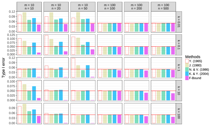
Figure 1: Type I errors of five testing methods for the multivariate Behrens–Fisher problem under different parameter settings, with each setting displayed in one sub-plot. The significance level is set to $\alpha=0.05$, indicated by the horizontal lines in each sub-plot, and the height of the bars stands for the Type I error. The first four methods are existing solutions to the problem, and the one labeled with “F-Bound” is the approach based on (7).

This phenomenon is even more clear under the $\alpha=0.01$ situation, as is shown in Figure 2. Under some circumstances the existing methods inflate the Type I error more than four times, which may cause unreliable conclusions in real applications. Same as the previous case, the F-Bound method is always valid despite its conservativeness.

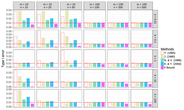
Figure 2: The same plot as Figure 1 but with significance level $\alpha=0.01$.

To summarize, the simulation study indicates that the theoretical result obtained in this article is useful to derive a testing procedure for the multivariate Behrens–Fisher problem that guarantees the Type I error control, which is crucial for many scientific studies.

5 Discussion and Conclusion

In this article we have revisited the multivariate Behrens–Fisher problem with the proportional covariances assumption, and have derived finite-sample lower and upper bounds for the null distribution of the test statistic. This result extends the previous work by Hsu (1938) for the univariate case and Eaton & Olshen (1972) for the two-dimensional case, and can be used to create a testing procedure that strongly controls the Type I error for the multivariate Behrens–Fisher problem.

It is true that the proportional covariances assumption (1) is a moderately strong restriction, and one may hope to verify the result for the most general forms of $\Sigma_{1}$ and $\Sigma_{2}$. In this article, this assumption is made based on the following two considerations. First, the original motivation of this article was to generalize Theorem 3.1 of Eaton & Olshen (1972), about the stochastic ordering of a series of random quotients, from two-dimension to any finite dimension. However, the test statistic for the most general Behrens–Fisher problem does not belong to this type of random quotient. Second, the technical difficulty of the general case is expected to be formidable. As can be seen from Lemma 2, there exists some concavity property for the proportional covariances case, which greatly helps proving the bounds. However, many examples can be given to show that such properties are totally destroyed in the general case, so some more advanced techniques need to be developed in order to fully solve the general situation. We leave this possibility for future research.

Appendix A Appendix

A.1 Proof of Lemma 1

Proof.

Since $\theta_{1},\ldots,\theta_{p}$ are exchangeable in $F(t;\theta)$, we will prove the case for $i=1,j=2$ without loss of generality. Define the random variable $T_{12}=Z_{1}^{2}/\theta_{1}+Z_{2}^{2}/\theta_{2}$ with the distribution function $F_{12}(t;\theta_{1},\theta_{2})$, and let $\phi(x)$ and $\Phi(x)$ denote the density function and distribution function of $N(0,1)$, respectively, then

$$F_{12}(t;\theta_{1},\theta_{2}) =\int_{-(\theta_{2}t)^{1/2}}^{(\theta_{2}t)^{1/2}}\mathrm{pr}(Z_{1}^{2}/\theta_{1}+s^{2}/\theta_{2}\leq t)\phi(s)\mathrm{d}s$$

$$=2\int_{0}^{(\theta_{2}t)^{1/2}}\left\{2\Phi\left(\left\{\theta_{1}(t-s^{2}/\theta_{2})\right\}^{1/2}\right)-1\right\}\phi(s)\mathrm{d}s$$

$$=4\int_{0}^{(\theta_{2}t)^{1/2}}\Phi\left(\left\{\theta_{1}(t-s^{2}/\theta_{2})\right\}^{1/2}\right)\phi(s)\mathrm{d}s-2\Phi((\theta_{2}t)^{1/2})+1,$$

$$\frac{\partial F_{12}(t;\theta_{1},\theta_{2})}{\partial\theta_{1}} =2\int_{0}^{(\theta_{2}t)^{1/2}}(t-s^{2}/\theta_{2})^{1/2}\theta_{1}^{-1/2}\phi\left(\left\{\theta_{1}(t-s^{2}/\theta_{2})\right\}^{1/2}\right)\phi(s)\mathrm{d}s>0.$$ (8)

Moreover, using the fact that $\phi^{\prime}(x)=-x\phi(x)$, we have

$$\frac{\partial^{2}F_{12}(t;\theta_{1},\theta_{2})}{\partial\theta_{1}^{2}}$$

$$= -\int_{0}^{(\theta_{2}t)^{1/2}}\left\{\left(t-s^{2}\theta_{2}^{-1}\right)^{3/2}\theta_{1}^{-1/2}+\left(t-s^{2}\theta_{2}^{-1}\right)^{\frac{1}{2}}\theta_{1}^{-3/2}\right\}\phi\left(\left\{\theta_{1}(t-s^{2}\theta_{2}^{-1})\right\}^{1/2}\right)\phi(s)\mathrm{d}s<0.$$

Let $\tilde{f}(t;\theta_{3},\ldots,\theta_{p})$ be the density function of $\tilde{T}=\sum_{i=3}^{p}Z_{i}^{2}/\theta_{i}$, and then $T_{\theta}=T_{12}+\tilde{T}$ has the distribution function $F(t;\theta)=\int_{0}^{t}F_{12}(s;\theta_{1},\theta_{2})\tilde{f}(t-s;\theta_{3},\ldots,\theta_{p})\mathrm{d}s$. Taking the partial derivatives with respect to $\theta_{1}$ on both sides, we have $f_{1}(t;\theta)=\int_{0}^{t}\left(\partial F_{12}(s;\theta_{1},\theta_{2})/\partial\theta_{1}\right)\tilde{f}(t-s;\theta_{3},\ldots,\theta_{p})\mathrm{d}s>0$ and $g_{1}(t;\theta)=\int_{0}^{t}\left(\partial^{2}F_{12}(s;\theta_{1},\theta_{2})/\partial\theta_{1}^{2}\right)\tilde{f}(t-s;\theta_{3},\ldots,\theta_{p})\mathrm{d}s<0$, which prove the statements a) and b).

Now let $h(\theta_{1},\theta_{2})=\partial F_{12}(t;\theta_{1},\theta_{2})/\partial\theta_{1}$ as in (8), and fix $0<a<b$ with $r=b/a>1$. With change of variables $u=s(bt)^{-1/2}$ followed by $\rho=\arcsin(u)$, we obtain

$$h(a,b) =2r^{1/2}t\int_{0}^{1}(1-u^{2})^{1/2}\phi((at)^{1/2}(1-u^{2})^{1/2})\phi((bt)^{1/2}u)\mathrm{d}u$$

$$=r^{1/2}t\pi^{-1}\int_{0}^{1}(1-u^{2})^{1/2}\exp\left\{-at(1-u^{2})/2-btu^{2}/2\right\}\mathrm{d}u$$

$$=r^{1/2}t\pi^{-1}\int_{0}^{\pi/2}\cos^{2}\rho\exp(-at\cos^{2}\rho/2-bt\sin^{2}\rho/2)\mathrm{d}\rho\equiv r^{1/2}t\pi^{-1}I_{ab}.$$

Similarly, by switching the order of $a$ and $b$ and with another change of variable $\eta=\pi/2-\rho$, it follows that

$$h(b,a)=r^{-1/2}t\pi^{-1}\int_{0}^{\pi/2}\sin^{2}\rho\exp(-at\cos^{2}\eta/2-bt\sin^{2}\eta/2)\mathrm{d}\eta\equiv r^{-1/2}t\pi^{-1}I_{ba}.$$

Therefore,

$$h(a,b)-h(b,a)$$

$$\geq t\pi^{-1}(I_{ab}-I_{ba})=t\pi^{-1}\int_{0}^{\pi/2}\cos(2\rho)\exp(-at\cos^{2}\rho/2-bt\sin^{2}\rho/2)\mathrm{d}\rho$$

$$=t\pi^{-1}\exp\{-(a+b)t/4\}\int_{0}^{\pi/2}\cos(2\rho)\exp\{(b-a)t\cos(2\rho)/4\}\mathrm{d}\rho$$

$$=(b-a)t^{2}(8\pi)^{-1}\exp\{-(a+b)t/4\}\int_{0}^{\pi/2}\sin^{2}(2\rho)\exp\{(b-a)t\cos(2\rho)/4\}\mathrm{d}\rho>0.$$ (9)

Now for $f_{2}(t;\theta)$, let $\theta_{ab}=(a,b,\theta_{3},\ldots,\theta_{p})$ and $\theta_{ba}=(b,a,\theta_{3},\ldots,\theta_{p})$, and then by symmetry we have $f_{2}(t;\theta_{ab})=f_{1}(t;\theta_{ba})$. Hence as a consequence of (9), we finally get

$$f_{1}(t;\theta_{ab})-f_{2}(t;\theta_{ab}) =f_{1}(t;\theta_{ab})-f_{1}(t;\theta_{ba})$$

$$=\int_{0}^{t}\{h(a,b)-h(b,a)\}\tilde{f}(t-s;\theta_{3},\ldots,\theta_{p})\mathrm{d}s>0,$$

whenever $0<a<b$, which concludes the proof of c). ∎

A.2 Proof of Lemma 2

Proof.

For simplicity we omit the parameters $t,M_{1},$ and $M_{2}$ in $h(\cdot)$ when no confusion is caused. Let $M(\lambda)=\lambda M_{1}+(1-\lambda)M_{2}$ be a matrix-valued function dependent on $\lambda$, and assume its eigen decomposition is $M(\lambda)=\Gamma(\lambda)D(\lambda)\Gamma(\lambda)^{\mathrm{T}}$, where $D(\lambda)=\mathrm{diag}\left\{d_{1}(\lambda),\ldots,d_{p}(\lambda)\right\}$ contains the sorted eigenvalues $d_{1}(\lambda)\geq\cdots\geq d_{p}(\lambda)>0$, and $\Gamma(\lambda)=(\gamma_{1}(\lambda),\ldots,\gamma_{p}(\lambda))$ are the associated eigenvectors. Again we will omit the $\lambda$ arguments in the relevant quantities above whenever appropriate.

Since $M^{-1}=\Gamma D^{-1}\Gamma^{\mathrm{T}}$, we have $h(\lambda)=\mathrm{pr}(Z^{\mathrm{T}}\Gamma D^{-1}\Gamma^{\mathrm{T}}Z\leq t)=\mathrm{pr}(Z^{\mathrm{T}}D^{-1}Z\leq t)$. The second identity holds since $\Gamma^{\mathrm{T}}Z\sim N(0,\Gamma^{\mathrm{T}}\Gamma),\Gamma^{\mathrm{T}}\Gamma=I_{p}$ and thus $Z\overset{d}{=}\Gamma^{\mathrm{T}}Z$. Therefore, using the notations in Lemma 1, we have $h(\lambda)=\mathrm{pr}(\sum_{i=1}^{p}Z_{i}^{2}/d_{i}\leq t)=F(t;\delta)$ where $\delta=(d_{1},\ldots,d_{p})$. As a result,

$$h^{\prime\prime}(\lambda)=\sum_{i=1}^{p}\left[g_{i}(t;\delta)\left(\frac{\partial d_{i}}{\partial\lambda}\right)^{2}+f_{i}(t;\delta)\left(\frac{\partial^{2}d_{i}}{\partial\lambda^{2}}\right)\right],$$ (10)

where $f_{i}(t;\delta)$ and $g_{i}(t;\delta)$ are also defined in Lemma 1.

Theorem 9 and Theorem 10 of Lancaster (1964) provide explicit expressions for $\partial^{2}d_{i}/\partial\lambda^{2}$, where the former assumes $d_{i}$’s are distinct while the latter considers multiplicity of eigenvalues. For now we shall assume that $d_{i}$’s are all distinct for brevity of the proof. The same technique applies to the more general case.

Let $M^{(k)}$ be the $k$th derivative of $M$ with respect to $\lambda$, then clearly $M^{(1)}=M_{1}-M_{2}$ and $M^{(2)}=O$ where $O$ is the zero matrix. Also define $p_{ij}=\gamma_{i}^{\mathrm{T}}M^{(1)}\gamma_{j}=p_{ji}$, then according to Theorem 9 of Lancaster (1964),

$$\frac{\partial^{2}d_{i}}{\partial\lambda^{2}}=2\sum_{\begin{subarray}{c}k=1\\ k\neq i\end{subarray}}^{p}\frac{p_{ik}p_{ki}}{d_{i}-d_{k}}=2\sum_{\begin{subarray}{c}k=1\\ k\neq i\end{subarray}}^{p}\frac{p_{ik}^{2}}{d_{i}-d_{k}}.$$

Now consider the cumulative sum of eigenvalues from the bottom, defined as $c_{i}=\sum_{j=i}^{p}d_{j}$, whose second derivative is given by

$$\frac{\partial^{2}c_{i}}{\partial\lambda^{2}} =\sum_{j=i}^{p}\frac{\partial^{2}d_{j}}{\partial\lambda^{2}}=2\sum_{j=i}^{p}\sum_{\begin{subarray}{c}k=1\\ k\neq j\end{subarray}}^{p}\frac{p_{jk}^{2}}{d_{j}-d_{k}}=2\sum_{j=i}^{p}\left(\sum_{k=1}^{i-1}\frac{p_{jk}^{2}}{d_{j}-d_{k}}+\sum_{\begin{subarray}{c}k=i\\ k\neq j\end{subarray}}^{p}\frac{p_{jk}^{2}}{d_{j}-d_{k}}\right)$$

$$=2\sum_{j=i}^{p}\sum_{k=1}^{i-1}\frac{p_{jk}^{2}}{d_{j}-d_{k}}+\sum_{\begin{subarray}{c}j,k\geq i\\ j\neq k\end{subarray}}\frac{p_{jk}^{2}}{d_{j}-d_{k}}.$$ (11)

For $j\neq k$, $p_{jk}^{2}(d_{j}-d_{k})^{-1}+p_{kj}^{2}(d_{k}-d_{j})^{-1}=0$, so the second term in (11) is zero. For the first term, since $k<j$ and hence $d_{j}<d_{k}$, we conclude that $\partial^{2}c_{i}/\partial\lambda^{2}<0$.

With this result, $h^{\prime\prime}(\lambda)$ in (10) can be written as

$$h^{\prime\prime}(\lambda) =\sum_{i=1}^{p}g_{i}(t;\delta)\left(\frac{\partial d_{i}}{\partial\lambda}\right)^{2}+\sum_{i=1}^{p}f_{i}(t;\delta)\left(\frac{\partial^{2}d_{i}}{\partial\lambda^{2}}\right)$$

$$<\sum_{i=1}^{p}f_{i}(t;\delta)\left(\frac{\partial^{2}d_{i}}{\partial\lambda^{2}}\right)=\sum_{i=1}^{p}\tilde{f}_{i}(t;\delta)\left(\frac{\partial^{2}c_{i}}{\partial\lambda^{2}}\right),$$ (12)

where $\tilde{f}_{1}=f_{1}$ and $\tilde{f}_{i}=f_{i}-f_{i-1}$ for $i\geq 2$. The inequality in (12) holds since $g_{i}(t;\delta)<0$ by part b) of Lemma 1. Moreover, since $d_{1}\geq\cdots\geq d_{p}$, we have $f_{1}\leq\cdots\leq f_{p}$ and thus $\tilde{f}_{i}\geq 0$ by part a) and c) of Lemma 1. This implies that $h^{\prime\prime}(\lambda)<0$ and hence concludes the proof. ∎

References

• Christensen & Rencher (1997) Christensen, W. F. & Rencher, A. C. (1997). A comparison of type i error rates and power levels for seven solutions to the multivariate behrens-fisher problem. Communications in Statistics-Simulation and Computation 26, 1251–1273.
• Eaton & Olshen (1972) Eaton, M. L. & Olshen, R. A. (1972). Random quotients and the behrens-fisher problem. The Annals of Mathematical Statistics 43, 1852–1860.
• Fisher (1935) Fisher, R. A. (1935). The fiducial argument in statistical inference. Annals of Human Genetics 6, 391–398.
• Hayter (2013) Hayter, A. (2013). A new procedure for the behrens–fisher problem that guarantees confidence levels. Journal of Statistical Theory and Practice 7, 515–536.
• Hsu (1938) Hsu, P. (1938). Contribution to the theory of "student’s" t-test as applied to the problem of two samples. Statistical Research Memoirs 2, 1–24.
• Johansen (1980) Johansen, S. (1980). The welch-james approximation to the distribution of the residual sum of squares in a weighted linear regression. Biometrika 67, 85–92.
• Kim & Cohen (1998) Kim, S.-H. & Cohen, A. S. (1998). On the behrens-fisher problem: a review. Journal of Educational and Behavioral Statistics 23, 356–377.
• Krishnamoorthy & Yu (2004) Krishnamoorthy, K. & Yu, J. (2004). Modified nel and van der merwe test for the multivariate behrens–fisher problem. Statistics & probability letters 66, 161–169.
• Lancaster (1964) Lancaster, P. (1964). On eigenvalues of matrices dependent on a parameter. Numerische Mathematik 6, 377–387.
• Magnus (1985) Magnus, J. R. (1985). On differentiating eigenvalues and eigenvectors. Econometric Theory 1, 179–191.
• Martin & Liu (2015) Martin, R. & Liu, C. (2015). Marginal inferential models: Prior-free probabilistic inference on interest parameters. Journal of the American Statistical Association 110, 1621–1631.
• Mickey & Brown (1966) Mickey, M. R. & Brown, M. B. (1966). Bounds on the distribution functions of the behrens-fisher statistic. The Annals of Mathematical Statistics 37, 639–642.
• Nel & Van der Merwe (1986) Nel, D. & Van der Merwe, C. (1986). A solution to the multivariate behrens-fisher problem. Communications in Statistics-Theory and Methods 15, 3719–3735.
• Nel et al. (1990) Nel, D. d., van der Merwe, C. A. & Moser, B. (1990). The exact distributions of the univariate and multivariate behrens-fisher statistics with a comparison of several solutions in the univariate case. Communications in Statistics-Theory and Methods 19, 279–298.
• Olkin & Marshall (2016) Olkin, I. & Marshall, A. W. (2016). Inequalities: Theory of majorization and its applications, vol. 143. Academic press.
• Pan et al. (2013) Pan, X., Xu, M., Hu, T. et al. (2013). Some inequalities of linear combinations of independent random variables: Ii. Bernoulli 19, 1776–1789.
• Rao (1973) Rao, C. R. (1973). Linear statistical inference and its applications, vol. 2. Wiley New York.
• Ruben (2002) Ruben, H. (2002). A simple conservative and robust solution of the behrens-fisher problem. Sankhyā: The Indian Journal of Statistics, Series A 64, 139–155.
• Satterthwaite (1946) Satterthwaite, F. E. (1946). An approximate distribution of estimates of variance components. Biometrics bulletin 2, 110–114.
• Scheffé (1943) Scheffé, H. (1943). On solutions of the behrens-fisher problem, based on the t-distribution. The Annals of Mathematical Statistics 14, 35–44.
• Scheffé (1970) Scheffé, H. (1970). Practical solutions of the behrens-fisher problem. Journal of the American Statistical Association 65, 1501–1508.
• Tsui & Weerahandi (1989) Tsui, K.-W. & Weerahandi, S. (1989). Generalized p-values in significance testing of hypotheses in the presence of nuisance parameters. Journal of the American Statistical Association 84, 602–607.
• Welch (1947) Welch, B. L. (1947). The generalization ofstudent’s’ problem when several different population variances are involved. Biometrika 34, 28–35.
• Yao (1965) Yao, Y. (1965). An approximate degrees of freedom solution to the multivariate behrens fisher problem. Biometrika 52, 139–147.